Dynamics of Predator-Prey Model with Fear Factor and Impulsive Nonlinear Effects

Abstract

In this article, we establish a predator–prey model with fear factor and impulsive nonlinear effects. The globally asymptotically stable conditions for the pest extinction periodic solution and the permanence condition of the formulated model are derived using Floquet theory and the comparison theorem of the impulsive differential equations. Simulations confirm the correctness of the theoretical results obtained in this paper and reveal the complex dynamics of the investigated model. Our results may assist pest control experts in determining the appropriate impulsive control period and release quantity of natural enemies for more effective pest management.

1. Introduction

The management of pests in agricultural production has been a subject of significant importance, as pests consistently result in economic losses for humans [1]. For instance, the management costs faced by farmers worldwide in the control of the diamondback moth, Plutella xylostella, a major pest of cabbage, cauliflower, and canola, are estimated at four to five billion dollars annually [2]. The incidence of yield loss in rice crops has increased as a result of the widespread occurrence of pests such as the brown plant hopper (Nilaparvata lugens) [3,4], rice leaffolder (Cnaphalocrocis medinalis Güenée) [5], and small brown planthopper (Laodelphax striatellus Fallen). The following pests were also observed: the rice hispa (Dicladispa armigera Oliver), the yellow stem borer (Scirpophaga incertulas L.), and the white-backed planthopper (Sogatella furcifera Horvath) [6]. These pests are a significant economic burden and cause hundreds of millions of dollars in losses annually. They also present a serious threat to food security in regions where rice is a primary food source [7]. It is estimated that up to 40% of the world’s food supply is already being lost to pests [8].

Consequently, humans have developed a variety of techniques, including the use of biological and chemical pesticides, the introduction of natural enemies, and the release of infected pest individuals, with the aim of controlling pests and safeguarding grain production [9,10,11]. This has prompted extensive research into pest management [12,13,14,15]. Initially, researchers posited that pest management was an ongoing, continuous process. Thus, they devised mathematical models of pest management incorporating continuous control measures [16,17]. However, the advancement of science has led to an understanding that the application of pest management measures, including the use of pesticides, the introduction of natural enemies, and the release of diseased pest individuals, cannot be considered as continuous processes within a system due to the potential for rapid changes to the state of the system [18]. Therefore, impulsive differential equations were introduced into pest management [12,13,19,20]. For example, Tian et al. [18] studied a prey–predator model with impulsive linear pesticide spraying and nonlinear release of natural enemies, which includes a regulating factor. Liu and Chen [21] studied the following prey–predator model with a Holling-II functional response and an impulsive release of predators.

$$\left\{\begin{array}{c}\left.\begin{array}{c}{\displaystyle \frac{d{x}_0\left(l\right)}{dl}}=a_0{x}_0\left(l\right)-b_0{x}_0^2\left(l\right)-{\displaystyle \frac{{\beta }_1{x}_0\left(l\right)x_1\left(l\right)}{1+{\alpha }_0{x}_0\left(l\right)}},\hfill \\ {\displaystyle \frac{d{x}_1\left(l\right)}{dl}}=-d_0{x}_1\left(l\right)+{\displaystyle \frac{k_0{\beta }_0{x}_0\left(l\right)x_1\left(l\right)}{1+{\alpha }_0{x}_0\left(l\right)}},\hfill \end{array}\right\}l\ne n\omega ,\hfill \\ \left.\begin{array}{c}\Delta x_0\left(l\right)=0,\hfill \\ \Delta x_1\left(l\right)=p_0,\hfill \end{array}\right\}l=n\omega ,\hfill \end{array}\right.$$

where $x_0\left(l\right)$ and $x_1\left(l\right)$ represent the prey and predator densities at time $l,$ respectively. ${\displaystyle \frac{{\beta }_1{x}_0\left(l\right)}{1+{\alpha }_0{x}_0\left(l\right)}}$ is a Holling-II predation functional response function of the predator. $p_0>0$ represents the impulsive nonlinear input of predators. $\omega >0$ denotes the impulsive period, and $\Delta x_i\left(l\right)=x_i\left(l^{+}\right)-x_i\left(l\right),$ $i=0,1.$ In order to illustrate the diverse pest management techniques employed by humans to enhance their efficacy, a series of pest management models with impulsive perturbations were introduced. For example, in [14], the authors studied a pest management system with impulsive linear insecticide spraying and nonlinear release of infective pests. Liu and Zhang [15] discussed a Lotka–Volterra prey–predator model with an impulsive nonlinear release of predators and a linear spraying of insecticides at fixed moments. In reference [19], the authors considered a switched predator–prey system with an impulsive linear spraying of pesticides and a nonlinear release of predators at different moments. The paper focused on the sublethal effects of pesticide residues on pests and their natural enemies. In particular, Zhang et al. [22] studied the following Beddington–DeAngelis functional response predator–prey integrated pest management system with impulsive linear insecticide spraying and nonlinear release of the natural enemies of pests.

$$\left\{\begin{array}{c}\left.\begin{array}{c}{\displaystyle \frac{dv\left(l\right)}{dl}}={\displaystyle \frac{{\beta }_2{b}_{1}u\left(l\right)v\left(l\right)}{A_1+k_{0}u\left(l\right)+k_{1}v\left(l\right)}}-w_{0}v\left(l\right),\hfill \\ {\displaystyle \frac{du\left(l\right)}{dl}}=u\left(l\right)(1-{\displaystyle \frac{u\left(l\right)}{K}})-{\displaystyle \frac{b_{1}u\left(l\right)v\left(l\right)}{A_1+k_{0}u\left(l\right)+k_{1}v\left(l\right)}},\hfill \end{array}\right\}l\ne (n+\xi -1)T,l\ne nT,\hfill \\ \left.\begin{array}{c}\Delta v\left(l\right)=-p_{2}v\left(l\right),\hfill \\ \Delta u\left(l\right)=-p_{1}u\left(l\right),\hfill \end{array}\right\}l=(n+\xi -1)T,\hfill \\ \left.\begin{array}{c}\Delta v\left(l\right)={\mu }_0,\hfill \\ \Delta u\left(l\right)=0,\hfill \end{array}\right\}l=nT,\hfill \end{array}\right.$$

(1)

where predator and prey density are $v\left(l\right)$ and $u\left(l\right)$ at time $l,$ respectively. The authors assume that the intrinsic growth rate of the prey population is $1.$ ${\displaystyle \frac{b_{1}u\left(l\right)v\left(l\right)}{A_1+k_{0}u\left(l\right)+k_{1}v\left(l\right)}},$ the predation behavior of predator, is a Beddington–DeAngelis functional response. $p_2>0$ and $p_1>0$ represent the death rate of the predator and prey due to pesticide spraying, respectively. ${\mu }_0>0$ denotes the release amount of the predator (the natural enemy of the pest) at time $l=nT.$ $T>0$ is the impulsive period, and $0<\xi <1$ is the time interval between the pulsed applications of control measures.

Fear-induced behavior plays a significant role in prey–predator dynamics [23,24,25]. The fear experienced by the prey, which is induced by the presence of the predators within an ecological ecosystem, is a crucial factor in determining the dynamic behavior of the interacting populations [26]. Furthermore, predator-induced fear can significantly affect the reproductive rate of prey. The experimental study conducted by Zanette et al. [27] indicates that predator-induced fear leads to a 40% reduction in the reproductive success of song sparrows’ offspring. Field observations by Elliott et al. [28] revealed that the reproductive rate of drosophila decreases in the presence of mantids. Therefore, the inclusion of the fear factor in the growth term of prey species is a more practical approach.

Based on the above literature review and considering the impact of fear on prey reproduction rates as well as the more realistic approach of nonlinear pesticide spraying, we propose a predator–prey pest management model that incorporates fear factor, impulsive nonlinear insecticide spraying, and the release of natural enemies of pests. In contrast to model (1), this model incorporates a Holling-II predation functional response. In order to prevent the detrimental impact of pesticides on a significant portion of newly released natural enemies and to guarantee the efficacy of pest control, the implementation of pesticide spraying and natural enemy release is scheduled at distinct fixed moments. The first step in the process is the application of pesticides, which are used to kill a substantial number of pests during outbreaks. This is followed by the introduction of natural enemies, which are released to control the remaining pests at the second stage of the process. Subsequently, the following integrated pest management model can be established.

$$\left\{\begin{array}{c}\left.\begin{array}{c}{\displaystyle \frac{d{y}_0\left(l\right)}{dl}}={\zeta }_0{y}_0\left(l\right)({\displaystyle \frac{1}{1+{\zeta }_1{y}_1\left(l\right)}}-{\displaystyle \frac{y_0\left(l\right)}{K_1}})-{\displaystyle \frac{{\delta }_0{y}_0\left(l\right)y_1\left(l\right)}{1+{\alpha }_0{y}_0\left(l\right)}},\hfill \\ {\displaystyle \frac{d{y}_1\left(l\right)}{dl}}=-a_0{y}_1\left(l\right)+{\displaystyle \frac{{\beta }_0{\delta }_0{y}_0\left(l\right)y_1\left(l\right)}{1+{\alpha }_0{y}_0\left(l\right)}},\hfill \end{array}\right\}l\ne (n+\gamma )\nu ,l\ne (n+1)\nu ,\hfill \\ \left.\begin{array}{c}\Delta y_0\left(l\right)=-{\displaystyle \frac{d_{max}{y}_0\left(l\right)}{{\alpha }_1+y_0\left(l\right)}}{y}_0\left(l\right),\hfill \\ \Delta y_1\left(l\right)=-d_2{y}_1\left(l\right),\hfill \end{array}\right\}l=(n+\gamma )\nu ,\hfill \\ \left.\begin{array}{c}\hfill \Delta y_0\left(l\right)=0,\\ \hfill \Delta y_1\left(l\right)=h_0,\end{array}\right\}l=(n+1)\nu ,\hfill \end{array}\right.$$

(2)

where the prey (pest) and predator (natural enemy) population densities are $y_0\left(l\right)$ and $y_1\left(l\right)$ at time $l,$ respectively. ${\zeta }_0>0$ represents the intrinsic rate of increase of the prey population. ${\zeta }_1>0$ denotes the fear level of the prey induced by the presence of predators. The predation of the predator follows the Holling-II functional response, given by ${\displaystyle \frac{{\delta }_0{y}_0\left(l\right)}{1+{\alpha }_0{y}_0\left(l\right)}}$ $({\alpha }_0>0,{\delta }_0>0).$ ${\beta }_0>0$ is the rate of conversion of nutrients into the reproduction rate of the predator. $a_0>0$ expresses the natural death rate of the predator. ${\displaystyle \frac{d_{max}{y}_0\left(l\right)}{{\alpha }_1+y_0\left(l\right)}}{y}_0\left(l\right)$ is impulsive nonlinear spraying pesticide at time $l=(n+\gamma )\nu .$ $0<d_{max}<1$ represents the maximum fatality rate of the predator because of pesticide, which can be controlled by adjusting the pesticide spraying. ${\alpha }_1>0$ is a half-saturation constant of the prey. It can be seen that $-{\displaystyle \frac{d_{max}{y}_0\left(l\right)}{{\alpha }_1+y_0\left(l\right)}}{y}_0\left(l\right)\to -d_{max}{y}_0\left(l\right)$ when $y_0\left(l\right)\to +\infty ,$ and $-{\displaystyle \frac{d_{max}{y}_0\left(l\right)}{{\alpha }_1+y_0\left(l\right)}}{y}_0\left(l\right)\to 0$ as $y_0\left(l\right)\to 0.$ $0<d_2<1$ denotes the death rate of the pest’s natural enemy due to spraying insecticide. $h_0>0$ is the release quantity of the predator (natural enemy) at time $l=(n+1)\nu .$ $0<\gamma <1$ is the time interval between two different impulse controls, and $\nu >0$ denotes the impulsive period.

The remainder of this paper is organized as follows. In Section 2, key preliminary results are presented to facilitate the subsequent analysis. The global asymptotic stability of the pest (prey) extinction periodic solution is derived in Section 3. In Section 4, the permanence of system (2) is analyzed. Furthermore, studying the complex dynamic behaviors of the system helps to predict the evolution of pest population and to design more effective pest control strategies, thereby reducing agriculture losses. Therefore, in Section 5, numerical simulations are presented to verify the correctness of the theoretical results and to explore the complex dynamics of the system (2) based on two more controllable parameters. We summarize our work in Section 6.

2. Preliminaries

Let $r={(r_0,r_1)}^T$ be the map defined on the right hand of system (2). Suppose $R_{+}=[0,+\infty ),$ $R_{+}^2=\{(x_0,x_1):x_0>0and{x}_1>0\},$ and $D_0\left(l\right)={(y_0\left(l\right),y_1\left(l\right))}^T:R_{+}\to R_{+}^2$. The solution of system (2), is a piecewise continuous function, which is continuous on the intervals $(n\nu ,(n+\gamma \left)\nu \right]$ and $\left(\right(n+\gamma )\nu ,(n+1\left)\nu \right],$ where $n\in Z_{+}.$ Meanwhile, all $y_0\left((n+\gamma ){\nu }^{+}\right)=\underset{l\to (n+\gamma ){\nu }^{+}}{lim}{y}_0\left(l\right),$ $y_1\left((n+\gamma ){\nu }^{+}\right)=\underset{l\to (n+\gamma ){\nu }^{+}}{lim}{y}_1\left(l\right),$ $y_0\left((n+1){\nu }^{+}\right)=\underset{l\to (n+1){\nu }^{+}}{lim}{y}_0\left(l\right),$ $y_1\left((n+1){\nu }^{+}\right)=\underset{l\to (n+1){\nu }^{+}}{lim}{y}_1\left(l\right)$ exist. The global existence and uniqueness of the solution to system (2) are ensured by the smoothness of r [29]. We have the following results according to system (2).

Lemma 1.

Suppose $D_0\left(l\right)$ is a solution of system (2) with $D_0\left(0^{+}\right)\ge 0$. We can derive $D_0\left(l\right)\ge 0$ for all $l\ge 0,$ and we can derive $D_0\left(l\right)>0$ for all $l\ge 0$ when $D_0\left(0^{+}\right)>0.$

Lemma 2.

There exists a constant $R_0>0$ such that $y_0\left(l\right)\le R_0$ and $y_1\left(l\right)\le R_0$ for l large enough.

Proof. 

Suppose $W_0\left(l\right)={\beta }_0{y}_0\left(l\right)+y_1\left(l\right).$ In accordance with the definition of upper right derivative in [15], when $l\ne (n+\gamma )\nu$ and $l\ne (n+1)\nu ,$ we obtain

$$D^{+}{W}_0\left(l\right)+\delta W_0\left(l\right)\le -{\displaystyle \frac{{\beta }_0{\zeta }_0}{K_1}}{y}_0^2\left(l\right)+{\beta }_0({\zeta }_0+\delta )y_0\left(l\right)+(\delta -a_0)y_1\left(l\right)\le R_1.$$

If $l=(n+\gamma )\nu ,$ we have

$$W_0\left((n+\gamma ){\nu }^{+}\right)={\beta }_0{y}_0\left((n+\gamma )\nu \right)(1-{\displaystyle \frac{d_{max}{y}_0\left((n+\gamma )\nu \right)}{{\alpha }_1+y_0\left((n+\gamma )\nu \right)}})+(1-d_2)y_1\left((n+\gamma )\nu \right)\le W_0\left((n+\gamma )\nu \right).$$

If $l=(n+1)\nu ,$ we derive

$$W_0\left((n+1){\nu }^{+}\right)={\beta }_0{y}_0\left((n+1)\nu \right)+y_1\left((n+1)\nu \right)+h_0=W_0\left((n+1)\nu \right)+h_0.$$

Therefore, we obtain

$$\left\{\begin{array}{c}{D}^{+}{W}_0\left(l\right)\le -\delta W_0\left(l\right)+R_1,l\ne (n+1)\nu ,\hfill \\ W_0\left((n+1){\nu }^{+}\right)=W_0\left((n+1)\nu \right)+h_0,l=(n+1)\nu .\hfill \end{array}\right.$$

Furthermore, we have

$$W_0\left(l\right)\le W_0\left(0^{+}\right)e^{-\delta l}+{\displaystyle \frac{R_1}{\delta }}(1-e^{-\delta l})+{\displaystyle \frac{h_0(1-e^{-\delta l})}{1-e^{-\delta \nu }}}\to {\displaystyle \frac{R_1}{\delta }}+{\displaystyle \frac{h_0}{1-e^{-\delta \nu }}}asl\to +\infty .$$

Hence, $W_0\left(l\right)$ is uniformly ultimately bounded. There exists an $R_0>0$ such that $y_0\left(l\right)\le R_0$ and $y_1\left(l\right)\le R_0$ in view of the definition of $W_0\left(l\right).$ □

In accordance with system (2), the following subsystem can be derived

$$\left\{\begin{array}{c}{\displaystyle \frac{d{y}_1\left(l\right)}{dl}}=-a_0{y}_1\left(l\right),l\ne (n+\gamma )\nu ,l\ne (n+1)\nu ,\hfill \\ \Delta y_1\left(l\right)=-d_2{y}_1\left(l\right),l=(n+\gamma )\nu ,\hfill \\ \Delta y_1\left(l\right)=h_0,l=(n+1)\nu .\hfill \end{array}\right.$$

(3)

The stroboscopic map of system (3) is given by

$$y_1\left((n+1){\nu }^{+}\right)=(1-d_2)e^{-a_0\nu }{y}_1\left(n{\nu }^{+}\right)+h_0,$$

which has a fixed point $y_1^{*}={\displaystyle \frac{h_0}{1-(1-d_2)e^{-a_0\nu }}}.$ Let $y_1\left(n{\nu }^{+}\right)=y_n.$ Subsequently,

$$y_{n+1}=o\left(y_n\right)=(1-d_2)e^{-a_0\nu }{y}_n+h_0,$$

$|{\displaystyle \frac{do\left(y_n\right)}{d{y}_n}}{|}_{y_n=y_1^{*}}|=(1-d_2)e^{-a_0\nu }<1.$ Hence, $y_1^{*}$ is locally asymptotically stable. Moreover,

$$\left|y_{n+1}-y_1^{*}\right|=(1-d_2)e^{-a_0\nu }\left|y_n-y_1^{*}\right|\to 0asn\to +\infty .$$

That is, the fixed point $y_1^{*}$ is globally asymptotically stable. Therefore, we have the following lemma.

Lemma 3.

The periodic solution $\overline{y_1^{*}\left(l\right)}$ of system (3) is globally asymptotically stable, where

$$\overline{y_1^{*}\left(l\right)}=\left\{\begin{array}{c}{y}_1^{*}{e}^{-a_0(l-n\nu )},l\in (n\nu ,(n+\gamma )\nu ],\hfill \\ (1-d_2)e^{-a_0\gamma \nu }{y}_1^{*}{e}^{-a_0(l-(n+\gamma )\nu )},l\in ((n+\gamma )\nu ,(n+1)\nu ].\hfill \end{array}\right.$$

In this paper, we assume that

(P₁)

${\zeta }_0\nu +{\displaystyle \frac{{\zeta }_0}{a_0}}ln{\displaystyle \frac{A}{B}}<{\displaystyle \frac{{\delta }_0{y}_1^{*}}{a_0}}(1-e^{-a_0\gamma \nu })+{\displaystyle \frac{{\delta }_0{y}_1^{*}(1-d_2)}{a_0}}(e^{-a_0\gamma \nu }-e^{-a_0\nu }),$

(P₂)

${\zeta }_0\nu <{\displaystyle \frac{{\delta }_0{y}_1^{*}}{a_0}}(1-e^{-a_0\gamma \nu })+{\displaystyle \frac{{\delta }_0{y}_1^{*}(1-d_2)}{d}}(e^{-a_0\gamma \nu }-e^{-a_0\nu }),K_1{\alpha }_0\le 1,$

(P₃)

${\zeta }_0\nu +{\displaystyle \frac{{\zeta }_0}{a_0}}ln{\displaystyle \frac{A}{B}}>{\displaystyle \frac{{\delta }_0{y}_1^{*}}{a_0}}(1-e^{-a_0\gamma \nu })+{\displaystyle \frac{{\delta }_0{y}_1^{*}(1-d_2)}{a_0}}(e^{-a_0\gamma \nu }-e^{-a_0\nu }),$

$$A=(1+{\zeta }_1{y}_1^{*}{e}^{-a_0\gamma \nu })(1+{\zeta }_1(1-d_2)y_1^{*}{e}^{-a_0\nu }),B=(1+{\zeta }_1{y}_1^{*})(1+{\zeta }_1(1-d_2)y_1^{*}).$$

3. Global Stability

Theorem 1.

When condition $P_1$ holds true, the pest elimination periodic solution $(0,\overline{y_1^{*}\left(l\right)})$ is locally asymptotically stable.

Proof. 

Assuming that $w_1\left(l\right)=y_0\left(l\right)$ and $w_2\left(l\right)=y_1\left(l\right)-\overline{y_1^{*}\left(l\right)},$ a linearized system can be derived for system (2).

$$\left(\begin{array}{c}{\displaystyle \frac{d{w}_1\left(l\right)}{dl}}\\ {\displaystyle \frac{d{w}_2\left(l\right)}{dl}}\end{array}\right)=\left(\begin{array}{cc}{\displaystyle \frac{{\zeta }_0}{1+{\zeta }_1\overline{y_1^{*}\left(l\right)}}}-{\delta }_0\overline{y_1^{*}\left(l\right)}& 0\\ {\beta }_0{\delta }_0\overline{y_1^{*}\left(l\right)}& -a_0\end{array}\right)\left(\begin{array}{c}{w}_1\left(l\right)\\ w_2\left(l\right)\end{array}\right),l\ne (n+\gamma )\nu ,l\ne (n+1)\nu .$$

The fundamental solution matrixes are denoted by

$${\psi }_1\left(l\right)=\left(\begin{array}{cc}{e}^{{\int }_{n\nu }^l({\displaystyle \frac{{\zeta }_0}{1+{\zeta }_1\overline{y_1^{*}\left(l\right)}}}-{\delta }_0\overline{y_1^{*}\left(l\right)})dl}& 0\\ {\aleph }_1& e^{-a_0(l-n\nu )}\end{array}\right),l\in (n\nu ,(n+\gamma )\nu ],$$

and

$${\psi }_2\left(l\right)=\left(\begin{array}{cc}{e}^{{\int }_{(n+\gamma )\nu }^l({\displaystyle \frac{{\zeta }_0}{1+{\zeta }_1\overline{y_1^{*}\left(l\right)}}}-{\delta }_0\overline{y_1^{*}\left(l\right)})dl}& 0\\ {\aleph }_2& e^{-a_0(l-(n+\gamma )\nu )}\end{array}\right),l\in ((n+\gamma )\nu ,(n+1)\nu ].$$

The exact forms of ${\aleph }_1$ and ${\aleph }_2$ are not required to be computed, as the following analysis does not depend on them. For $l=(n+\gamma )\nu ,$ we have

$$\left(\begin{array}{c}{w}_1\left((n+\gamma ){\nu }^{+}\right)\\ w_2\left((n+\gamma ){\nu }^{+}\right)\end{array}\right)=\left(\begin{array}{cc}1& 0\\ 0& 1-d_2\end{array}\right)\left(\begin{array}{c}{w}_1\left((n+\gamma )\nu \right)\\ w_2\left((n+\gamma )\nu \right)\end{array}\right).$$

For $l=(n+1)\nu ,$ we derive

$$\left(\begin{array}{c}{w}_1\left((n+1){\nu }^{+}\right)\\ w_2\left((n+1){\nu }^{+}\right)\end{array}\right)=\left(\begin{array}{cc}1& 0\\ 0& 1\end{array}\right)\left(\begin{array}{c}{w}_1\left((n+1)\nu \right)\\ w_2\left((n+1)\nu \right)\end{array}\right).$$

We obtain the following matrix,

$$\phi ={\psi }_2\left(\nu \right)\left(\begin{array}{cc}1& 0\\ 0& 1-d_2\end{array}\right){\psi }_1\left(\gamma \nu \right),$$

which determines the local stability of $(0,\overline{y_1^{*}\left(l\right)})$ by its eigenvalues. The eigenvalues of $\phi$ are

$${\lambda }_1=exp\{{\zeta }_0\nu +{\displaystyle \frac{{\zeta }_0}{a_0}}ln{\displaystyle \frac{A}{B}}-{\displaystyle \frac{{\delta }_0{y}_1^{*}}{a_0}}(1-e^{-a_0\gamma \nu })-{\displaystyle \frac{{\delta }_0{y}_1^{*}(1-d_2)}{a_0}}(e^{-a_0\gamma \nu }-e^{-a_0\nu })\},$$

$${\lambda }_2=(1-d_2)e^{-a_0\nu }.$$

Obviously, $|{\lambda }_1|<1$ if $P_1$ holds, and $|{\lambda }_2|<1.$ Based on the Floquet theory [30], the pest extinction periodic solution $(0,\overline{y_1^{*}\left(l\right)})$ of system (2) is locally asymptotically stable if condition $P_1$ holds. □

Theorem 2.

When $P_2$ holds true, $(0,\overline{y_1^{*}\left(l\right)})$ is globally asymptotically stable.

Proof. 

In view of Lemma 3, for any positive constant ${\tau }_0$ and sufficiently large $l,$ we can obtain $y_1\left(l\right)\ge \overline{y_1^{*}\left(l\right)}-{\tau }_0.$ Suppose $y_1\left(l\right)\ge \overline{y_1^{*}\left(l\right)}-{\tau }_0$ for $l\ge 0$ holds true. From system (2), we derive

$$\dot{y_0\left(l\right)}={\zeta }_0{y}_0\left(l\right)({\displaystyle \frac{1}{1+{\zeta }_1{y}_1\left(l\right)}}-{\displaystyle \frac{y_0\left(l\right)}{K_1}})-{\displaystyle \frac{{\delta }_0{y}_0\left(l\right)y_1\left(l\right)}{1+{\alpha }_0{y}_0\left(l\right)}}\Rightarrow \dot{y_0}={\zeta }_0{y}_0({\displaystyle \frac{1}{1+{\zeta }_1{y}_1}}-{\displaystyle \frac{y_0}{K_1}})-{\displaystyle \frac{{\delta }_0{y}_0{y}_1}{1+{\alpha }_0{y}_0}}.$$

We claim that $p_1\left(y_0\right)={\displaystyle \frac{{\delta }_0{y}_0\left(l\right)}{1+{\alpha }_0{y}_0\left(l\right)}},$ $\dot{y_0}={\displaystyle \frac{d{y}_0}{dl}},$ $y_0=y_0\left(l\right)$ and $y_1=y_1\left(l\right).$ Therefore,

$${\int }_{y_{00}}^{y_0\left(l\right)}{\displaystyle \frac{1}{p_1\left(y_0\right)}}d{y}_0={\int }_{l_0}^l({\displaystyle \frac{{\zeta }_0{y}_0\left(v\right)(\frac{1}{1+{\zeta }_1{y}_1\left(v\right)}-\frac{y_0\left(v\right)}{K_1})}{p_1\left(y_0\left(v\right)\right)}}-y_1\left(v\right))dv,$$

${\int }_{y_{00}}^{y_0\left(l\right)}{\displaystyle \frac{1}{p_1\left(y_0\right)}}d{y}_0\to -\infty$ as $y_0\to 0$ due to $p_1\left(y_0\right)\approx p_1^{\prime }\left(0\right)y_0$ and $p_1^{\prime }\left(0\right)={\delta }_0>0$ for small enough $y_0.$

$$G\left(y_0\right)={\int }_{\eta }^{y_0}{\displaystyle \frac{1}{p_1\left(v\right)}}dv,$$

with $\eta >0,$ thus $y_0\left(l\right)\to 0$ if $G\left(y_0\right)\to -\infty$ as $l\to +\infty .$ That is, the pest tends to extinction when $G\left(y_0\right)\to -\infty$ as $l\to +\infty .$ Moreover,

$${\displaystyle \frac{dG\left(y_0\right)}{dl}}={\displaystyle \frac{\dot{y_0}}{p_1\left(y_0\right)}}={\displaystyle \frac{{\zeta }_0{y}_0(\frac{1}{1+{\zeta }_1{y}_1}-\frac{y_0}{K_1})}{p_1\left(y_0\right)}}-y_1.$$

On interval $\left(\right(n+\gamma )\nu ,(n+1+\gamma \left)\nu \right]$, we have

$$\begin{array}{cc}\hfill G\left(y_0\left((n+1+\gamma ){\nu }^{+}\right)\right)& \le G\left(y_0\left((n+\gamma ){\nu }^{+}\right)\right)+{\int }_{(n+\gamma )\nu }^{(n+1+\gamma )\nu }({\displaystyle \frac{{\zeta }_0{y}_0\left(v\right)(1-\frac{y_0\left(v\right)}{K_1})}{p_1\left(v\right)}})-(\overline{y_1^{*}\left(v\right)}-{\tau }_0)dv\hfill \\ & +{\int }_{y_0\left((n+1+\gamma )\nu \right)}^{y_0\left((n+1+\gamma ){\nu }^{+}\right)}{\displaystyle \frac{1}{p_1\left(v\right)}}dv\hfill \\ & \le G\left(y_0\left((n+\gamma ){\nu }^{+}\right)\right)+{\int }_{(n+\gamma )\nu }^{(n+1+\gamma )\nu }(M_0-(\overline{y_1^{*}\left(v\right)}-{\tau }_0))dv,\hfill \end{array}$$

$$M_0=\underset{y_0\ge 0}{sup}\{{\displaystyle \frac{{\zeta }_0{y}_0(1-\frac{y_0}{K_1})}{p_1\left(y_0\right)}}\}={\displaystyle \frac{{\zeta }_0}{{\delta }_0}},K_1{\alpha }_0\le 1.$$

When $l\in \left(\right(n+\gamma )\nu ,(n+1+\gamma \left)\nu \right],$ we have

$$\begin{array}{c}\hfill G\left(y_0\left(l\right)\right)-G\left(y_{00}\right)\le n{\int }_{\gamma \nu }^{(1+\gamma )\nu }(M_0-(\overline{y_1^{*}\left(v\right)}-{\tau }_0))dv+{\int }_{(n+\gamma )\nu }^l(M_0-(\overline{y_1^{*}\left(v\right)}-{\tau }_0))dv.\end{array}$$

If

$${\int }_{\gamma \nu }^{(1+\gamma )\nu }(M_0-(\overline{y_1^{*}\left(v\right)}-{\tau }_0))dv={\int }_{\gamma \nu }^{(1+\gamma )\nu }({\displaystyle \frac{{\zeta }_0}{{\delta }_0}}-(\overline{y_1^{*}\left(v\right)}-{\tau }_0))dv<0,$$

we can obtain $G\left(y_0\left(l\right)\right)\to -\infty$ as $l\to +\infty .$ That is, $y_0\left(l\right)\to 0$ as $l\to +\infty$ when $P_2$ holds.

By selecting a sufficiently small $0<{\tau }_1<{\displaystyle \frac{a_0}{{\beta }_0{\delta }_0}},$ there must exist an $n_1>0$ with $n_1\in Z_{+},$ $Z_{+}=\{1,2,3,...\}$ such that $y_0\left(l\right)\le {\tau }_1$ when $l\ge n_1\nu .$ Considering the following system with ${\upsilon }_1\left(n_1{\nu }^{+}\right)=y_1\left(n_1{\nu }^{+}\right)$,

$$\left\{\begin{array}{c}{\displaystyle \frac{d{\upsilon }_1\left(l\right)}{dl}}={\upsilon }_1\left(l\right)(-a_0+{\beta }_0{\delta }_0{\tau }_1),l\ne (n+\gamma )\nu ,l\ne (n+1)\nu ,\hfill \\ \Delta {\upsilon }_1\left(l\right)=-d_2{\upsilon }_1\left(l\right),l=(n+\gamma )\nu ,\hfill \\ \Delta {\upsilon }_1\left(l\right)=h_0,l=(n+1)\nu ,\hfill \end{array}\right.$$

(4)

in accordance with Lemma 3, we obtain ${\upsilon }_1\left(l\right)\to \overline{{\upsilon }_1^{*}\left(l\right)}$ as $l\to +\infty ,$ where $\overline{{\upsilon }_1^{*}\left(l\right)}$ is the periodic solution of system (4), and

$$\overline{{\upsilon }_1^{*}\left(l\right)}=\left\{\begin{array}{c}{\upsilon }_1^{*}exp\left\{(-a_0+{\beta }_0{\delta }_0{\tau }_1)(l-n\nu )\right\},l\in (n\nu ,(n+\gamma )\nu ],\hfill \\ (1-d_2){\upsilon }_1^{*}{e}^{(-a_0+{\beta }_0{\delta }_0{\tau }_1)\gamma \nu }exp\left\{(-a_0+{\beta }_0{\delta }_0{\tau }_1)(l-(n+\gamma )\nu )\right\},l\in ((n+\gamma )\nu ,(n+1)\nu ],\hfill \end{array}\right.$$

${\upsilon }_1^{*}={\displaystyle \frac{h_0}{1-(1-d_2)e^{(-a_0+\frac{{\beta }_0{\delta }_0{\tau }_1}{1+{\alpha }_0{\tau }_1})\nu }}}.$ Moreover, in view of system (2) and the comparison theorem of the impulsive differential equations [29], we obtain $y_1\left(l\right)\le {\upsilon }_1\left(l\right)\le \overline{{\upsilon }_1^{*}\left(l\right)}+{\tau }_0$ for l sufficiently large. Therefore, we have $\overline{y_1^{*}\left(l\right)}-{\tau }_0\le y_1\left(l\right)\le \overline{{\upsilon }_1^{*}\left(l\right)}+{\tau }_0$ for l sufficiently large. Let ${\tau }_1\to 0$. We have

$$\overline{y_1^{*}\left(l\right)}-{\tau }_0\le y_1\left(l\right)\le \overline{y_1^{*}\left(l\right)}+{\tau }_0.$$

That is, $|y_1\left(l\right)-\overline{y_1^{*}\left(l\right)}|\to 0$ as $l\to +\infty$. Thus, $(0,\overline{y_1^{*}\left(l\right)})$ is globally attractive. Based on the above analysis, we obtain that the pest-eradication periodic solution $(0,\overline{y_1^{*}\left(l\right)})$ of system (2) is globally asymptotically stable. □

4. Permanence

Definition 1.

System (2) is permanent if there exist constants $q_1>0,$ $q_2>0,$ $R_0>0$ and a finite time $l_0$ such that the solution $(y_0\left(l\right),y_1\left(l\right))$ of system (2) with $y_0\left(0^{+}\right)>0$ and $y_1\left(0^{+}\right)>0$ satisfies $q_2\le y_0\left(l\right)\le R_0$ and $q_1\le y_1\left(l\right)\le R_0$ for all $l\ge l_0.$

Theorem 3.

If $P_3$ holds, system (2) is permanent.

Proof. 

As demonstrated in Lemma 2, there exists a constant $R_0>0$ such that $y_0\left(l\right)\le R_0$ and $y_1\left(l\right)\le R_0$ for sufficiently large l. Consequently, in the following steps, it is only necessary to find positive constants $q_1$ and $q_2$ such that $y_0\left(l\right)\le q_2$ and $y_1\left(l\right)\le q_1$ for all sufficiently large l, which is in accordance with Definition 1.

From Lemma 3, we have, for sufficiently large l,

$$y_1\left(l\right)\ge \overline{y_1^{*}\left(l\right)}-{\tau }_0\ge (1-d_2)y_1^{*}{e}^{-a_0\nu }=q_1.$$

Next, we prove that there exists a positive constant $q_2$ such that $y_0\left(l\right)\ge q_2$ for sufficiently large l. Select a $q_2^{\prime }>0$ and ${\tau }_2>0$ such that $0<q_2^{\prime }<{\displaystyle \frac{a_0}{{\beta }_0{\delta }_0}}$ and ${\kappa }_1={\int }_{(n+\gamma )\nu }^{(n+1+\gamma )\nu }({\displaystyle \frac{{\zeta }_0}{1+{\zeta }_1(\overline{v_2\left(l\right)}+{\tau }_2)}}-{\displaystyle \frac{{\zeta }_0{q}_2^{\prime }}{K_1}}-{\delta }_0(\overline{v_2\left(l\right)}+{\tau }_2))dl+ln(1-{\displaystyle \frac{d_{max}{q}_2^{\prime }}{{\alpha }_1+q_2^{\prime }}})>0,$ where

$$\begin{array}{c}\hfill \overline{v_2\left(l\right)}=\left\{\begin{array}{c}{v}_2^{*}exp\left\{(-a_0+{\beta }_0{\delta }_0{q}_2^{\prime })(l-n\nu )\right\},l\in (n\nu ,(n+\gamma )\nu ],\hfill \\ (1-d_2)v_2^{*}exp\left\{(-a_0+{\beta }_0{\delta }_0{q}_2^{\prime })(l-n\nu )\right\},l\in ((n+\gamma )\nu ,(n+1)\nu ],\hfill \end{array}\right.\end{array}$$

and $v_2^{*}={\displaystyle \frac{h_0}{1-(1-d_2)exp\left\{(-a_0+{\beta }_0{\delta }_0{q}_2^{\prime })\nu \right\}}}$. It can be proved that there exists a ${\tau }_1^{\prime }>0$ such that $y_0\left({\tau }_1^{\prime }\right)\ge q_2^{\prime },$ otherwise, for all $l>0,$ we have $y_0\left(l\right)<q_2^{\prime }.$ Let $v_2\left(0^{+}\right)=y_1\left(0^{+}\right).$ Considering system

$$\left\{\begin{array}{c}{\displaystyle \frac{d{v}_2\left(l\right)}{dl}}=v_2\left(l\right)(-a_0+{\beta }_0{\delta }_0{q}_2^{\prime }),l\ne (n+\gamma )\nu ,l\ne (n+1)\nu ,\hfill \\ \Delta v_2\left(l\right)=-d_2{v}_2\left(l\right),l=(n+\gamma )\nu ,\hfill \\ \Delta v_2\left(l\right)=h_0,l=(n+1)\nu ,\hfill \end{array}\right.$$

(5)

we obtain that the periodic solution $\overline{v_2\left(l\right)}$ of system (5) is globally asymptotically stable from Lemma 3. Furthermore, for ${\tau }_2>0,$ $y_1\left(l\right)\le v_2\left(l\right)\le \overline{v_2\left(l\right)}+{\tau }_2$ for $l\ge L_1$ in accordance with the comparison theorem of the impulsive differential equations [29]. From system (2), we have

$$\left\{\begin{array}{c}{\displaystyle \frac{d{y}_0\left(l\right)}{dl}}\ge y_0\left(l\right)({\displaystyle \frac{{\zeta }_0}{1+{\zeta }_1(\overline{v_2\left(l\right)}+{\tau }_2)}}-{\displaystyle \frac{{\zeta }_0{q}_2^{\prime }}{K_1}}-{\delta }_0(\overline{v_2\left(l\right)}+{\tau }_2)),l\ne (n+\gamma )\nu ,\hfill \\ \Delta y_0\left(l\right)=-{\displaystyle \frac{d_{max}{y}_0\left(l\right)}{{\alpha }_1+y_0\left(l\right)}}{y}_0\left(l\right),l=(n+\gamma )\nu .\hfill \end{array}\right.$$

(6)

for $l\ge L_1.$ Suppose $M_1\nu >L_1.$ Integrating system (6) on $((n+\gamma )\nu ,(n+1+\gamma )\nu ],n\ge M_1,$ we have

$$\begin{array}{cc}\hfill y_0\left((n+1+\gamma ){\nu }^{+}\right)& \ge e^{{\kappa }_1}{y}_0\left((n+\gamma ){\nu }^{+}\right),\hfill \end{array}$$

that is, $y_0\left((M_1+r+\gamma ){\nu }^{+}\right)\ge e^{r{\kappa }_1}{y}_0\left((M_1+\gamma ){\nu }^{+}\right)\to +\infty$ as $r\to +\infty ,$ which is a contradiction. Therefore, there is a ${\tau }_1^{\prime }>0$ such that $y_0\left({\tau }_1^{\prime }\right)\ge q_2^{\prime }.$ Our goal is reached when $y_0\left(l\right)\ge q_2^{\prime }$ for all $l\ge {\tau }_1^{\prime }.$ Let $l^{*}=\underset{l\ge {\tau }_1^{\prime }}{inf}\{y_0\left(l\right)<q_2^{\prime }\}$. There are two cases for $l^{*}.$

Case 1: $l^{*}=(n_1+\gamma )\nu ,n_1\in Z_{+}.$ Then $y_0\left(l\right)\ge q_2^{\prime }$ for $l\in [{\tau }_1^{\prime },l^{*})$ and $y_0\left(l^{*}\right)=q_2^{\prime }.$ Select $n_2,n_3\in N$ such that

$${(1-{\displaystyle \frac{d_{max}{q}_2^{\prime }}{{\alpha }_1+q_2^{\prime }}})}^{n_2}{e}^{n_3{\kappa }_1}{e}^{n_2\kappa \nu }>1,$$

where $\kappa ={\displaystyle \frac{{\zeta }_0}{1+{\zeta }_1{R}_0}}-{\displaystyle \frac{{\zeta }_0{q}_2^{\prime }}{K_1}}-{\delta }_0{R}_0<0.$ Let $T_1=(n_2+n_3)\nu .$ There exists a $l_2\in [l^{*},l^{*}+T_1]$ such that $y_0\left(l_2\right)\ge q_2^{\prime }$; otherwise, we consider system (5). It can be derived that $y_1\left(l\right)\le v_2\left(l\right)\le \overline{v_2\left(l\right)}+{\tau }_2$ for $l^{*}+n_2\nu \le l\le l^{*}+T_1,$ which indicates that (6) holds true for $l\in [l^{*}+n_2\nu ,l^{*}+T_1],$ thus $y_0(l^{*}+T_1)\ge y_0(l^{*}+n_2\nu )e^{n_3{\kappa }_1}.$ From system (2), we derive

$$\left\{\begin{array}{c}{\displaystyle \frac{d{y}_0\left(l\right)}{dl}}\ge y_0\left(l\right)({\displaystyle \frac{{\zeta }_0}{1+{\zeta }_1{R}_0}}-{\displaystyle \frac{{\zeta }_0{q}_2^{\prime }}{K_1}}-{\delta }_0{R}_0),l\ne (n+\gamma )\nu ,\hfill \\ \Delta y_0\left(l\right)=-{\displaystyle \frac{d_{max}{y}_0\left(l\right)}{{\alpha }_1+y_0\left(l\right)}}{y}_0\left(l\right),l=(n+\gamma )\nu ,\hfill \end{array}\right.$$

(7)

integrating the above system on $[l^{*},l^{*}+n_2\nu ],$ thus $y_0(l^{*}+n_2\nu )\ge {(1-{\displaystyle \frac{d_{max}{q}_2^{\prime }}{{\alpha }_1+q_2^{\prime }}})}^{n_2}{q}_2^{\prime }{e}^{\kappa n_2\nu }.$ Moreover,

$$y_0(l^{*}+T_1)\ge {(1-{\displaystyle \frac{d_{max}{q}_2^{\prime }}{{\alpha }_1+q_2^{\prime }}})}^{n_2}{q}_2^{\prime }{e}^{\kappa n_2\nu }{e}^{n_3{\kappa }_1}>q_2^{\prime },$$

which is a contradiction. Suppose $\overline{l}=\underset{l\ge l^{*}}{inf}\{y_0\left(l\right)\ge q_2^{\prime }\}$. Subsequently, $y_0\left(\overline{l}\right)=q_2^{\prime },$ and $y_0\left(l\right)\ge {(1-{\displaystyle \frac{d_{max}{q}_2^{\prime }}{{\alpha }_1+q_2^{\prime }}})}^{n_2+n_3}{q}_2^{\prime }{e}^{\kappa (n_2+n_3)\nu }=q_2.$ For $l>\overline{l}$, the same discussion can be continued because $y_0\left(\overline{l}\right)\ge q_2^{\prime }.$ Therefore, $y_0\left(l\right)\ge q_2$ for $l>{\tau }_1^{\prime }.$

Case 2: $l^{*}\ne (n_1+\gamma )\nu ,n_1\in Z_{+}.$ Then $y_0\left(l\right)\ge q_2^{\prime }$ for $l\in [{\tau }_1^{\prime },l^{*})$ and $y_0\left(l^{*}\right)=q_2^{\prime }.$ Suppose $l^{*}\in ((n_1^{\prime }+\gamma )\nu ,(n_1^{\prime }+1+\gamma )\nu ),n_1^{\prime }\in Z_{+}.$ There are two cases.

Case 2 (a): $y_0\left(l\right)<q_2^{\prime }$ for all $l\in (l^{*},(n_1^{\prime }+1+\gamma )\nu ).$ Similar to Case 1, there exists a $l_2^{\prime }\in [(n_1^{\prime }+1+\gamma )\nu ,(n_1^{\prime }+1+\gamma )\nu +T_1]$ such that $y_0\left(l_2^{\prime }\right)\ge q_2^{\prime },$ we ignore it. Suppose $\tilde{l}=\underset{l\ge l^{*}}{inf}\{y_0\left(l\right)\ge q_2^{\prime }\}.$ For $l\in [l^{*},\tilde{l}),$ we have $y_0\left(l\right)\ge {(1-{\displaystyle \frac{d_{max}{q}_2^{\prime }}{{\alpha }_1+q_2^{\prime }}})}^{n_2+n_3}{q}_2^{\prime }{e}^{(n_2+n_3+1)\kappa \nu }=q_2.$ The same arguments can continue for $l>\tilde{l}$; thus, $y_0\left(l\right)\ge q_2$ for $l>{\tau }_1^{\prime }.$

Case 2 (b): There exists a $l^{\prime }\in (l^{*},(n_1^{\prime }+1+\gamma )\nu )$ such that $y_0\left(l^{\prime }\right)\ge q_2^{\prime }.$ Let $\widehat{l}=\underset{l\ge l^{*}}{inf}\{y_0\left(l\right)\ge q_2^{\prime }\}.$ For $l\in [l^{*},\widehat{l}),$ integrating system (7), it can be concluded that $y_0\left(l\right)\ge q_2^{\prime }{e}^{\kappa \nu }=q_2.$ The same discussion can continue for $l>\widehat{l}$ due to $y_0\left(\widehat{l}\right)\ge q_2^{\prime }$; thus, $y_0\left(l\right)\ge q_2$ for $l\ge {\tau }_1^{\prime }.$ □

5. Simulation and Discussion

In this section, in order to examine our results obtained in previous sections and to explore complex dynamic behaviors of the system, some numerical simulations are inserted. At first, we verify the condition of the pest-eradication periodic solution $(0,\overline{y_1^{*}\left(l\right)})$ globally asymptotically stable, and test the condition of permanence of system (2).

Suppose ${\zeta }_0=1,$ ${\zeta }_1=0.5,$ $K_1=2,$ ${\delta }_0=0.6,$ ${\alpha }_0=0.2,$ ${\beta }_0=0.65,$ $a_0=0.23,$ $d_{max}=0.6,$ ${\alpha }_1=0.1,$ $d_2=0.3,$ $h_0=2,$ $\nu =3,$ $\gamma =0.35.$ We obtain

$${\zeta }_0\nu =3<{\displaystyle \frac{{\delta }_0{y}_1^{*}}{a_0}}(1-e^{-a_0\gamma \nu })+{\displaystyle \frac{{\delta }_0{y}_1^{*}}{a_0}}(e^{-a_0\gamma \nu }-e^{-a_0\nu })=3.3228,K_1{\alpha }_0=0.4<1.$$

Condition of Theorem 2 holds. Thus, $(0,\overline{y_1^{*}\left(l\right)})$ is globally asymptotically stable (see Figure 1).

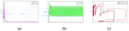
Figure 1. Global asymptotic stability of $(0,\overline{y_1^{*}\left(l\right)})$: (a) Time-series of $y_0\left(l\right).$ (b) Time-series of $y_1\left(l\right).$ (c) Phase portrait.

Set $h_0=0.5$ and maintain other parameters of system (2). We derive

$${\zeta }_0\nu +{\displaystyle \frac{{\zeta }_0}{a_0}}ln{\displaystyle \frac{(1+{\zeta }_1{y}_1^{*}{e}^{-a_0\gamma \nu })(1+{\zeta }_1(1-d_2)y_1^{*}{e}^{-a_0\nu })}{(1+{\zeta }_1{y}_1^{*})(1+{\zeta }_1(1-d_2)y_1^{*})}}=2.246,$$

$${\displaystyle \frac{{\delta }_0{y}_1^{*}}{a_0}}(1-e^{-a_0\gamma \nu })+{\displaystyle \frac{{\delta }_0{y}_1^{*}}{a_0}}(e^{-a_0\gamma \nu }-e^{-a_0\nu })=0.8307.$$

Clearly, $2.246>0.8307,$ which indicates that Theorem 3 holds true. Therefore, system (2) is permanent (see Figure 2).

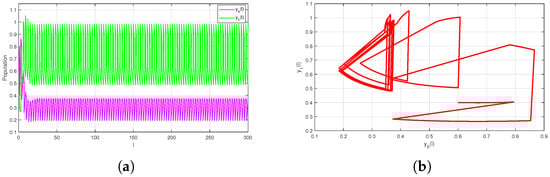
Figure 2. Permanence of system (2) with $(y_0\left(0\right),y_1\left(0\right))=(0.6,0.4)$: (a) Time-series of $y_0\left(l\right)$ and $y_1\left(l\right).$ (b) Phase portrait.

Next, we study complex dynamic behaviors of system (2). If we assume that the parameters of system (2) are ${\zeta }_0=7.5,$ ${\zeta }_1=0.5,$ $K_1=18,$ ${\delta }_0=0.77,$ ${\alpha }_0=0.04,$ $a_0=0.25,$ ${\beta }_0=0.49,$ $d_{max}=0.63,$ ${\alpha }_1=0.3,$ $d_2=0.4,$ $\gamma =0.65,$ $\nu =7.5,$ the bifurcation diagrams listed below about a parameter $h_0$, which transforms from $0.01$ to $21.01$, can be derived (see Figure 3). System (2) exhibits a rich variety of dynamic behaviors, including cycles, period-doubling cascades, chaos, and period-halving cascades. Corresponding examples are shown in Figure 4 and Figure 5.

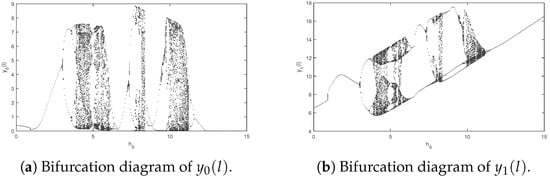
Figure 3. Bifurcation diagrams of system (2) about $h_0$ with $(y_0\left(0\right),y_1\left(0\right))=(0.6,0.4),$ $0.01\le h_0\le 21.01$.

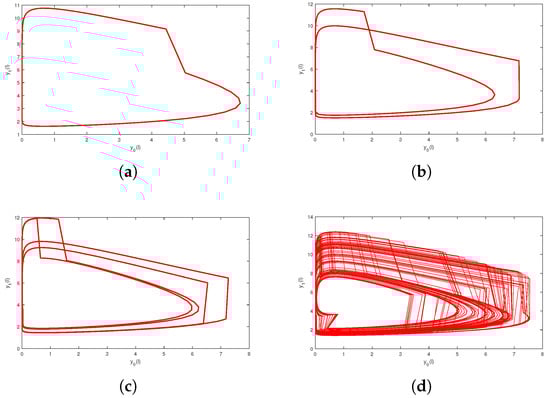
Figure 4. Period-doubling cascades lead to system into chaos: (a) Phase portrait of a $\nu -$periodic solution at $h_0=2.9.$ (b) Phase portrait of a $2\nu -$periodic solution at $h_0=3.3.$ (c) Phase portrait of a $4\nu -$periodic solution at $h_0=3.65.$ (d) Phase portrait of chaos at $h_0=4.1$.

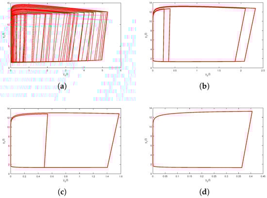
Figure 5. Period-halving cascades lead to a system from chaos into a $\nu -$periodic solution: (a) Phase portrait of chaos at $h_0=11.1.$ (b) Phase portrait of a $4\nu -$periodic solution at $h_0=11.35.$ (c) Phase portrait of a $2\nu -$periodic solution at $h_0=11.5.$ (d) Phase portrait of a $\nu -$periodic solution at $h_0=12$.

Next, we research the effect of the impulsive period $\nu$ for the studied system. Suppose parameters of system (2) are as follows: ${\zeta }_0=4.97,$ ${\zeta }_1=0.15,$ $K_1=20,$ ${\delta }_0=0.78,$ ${\alpha }_0=0.04,$ $a_0=0.27,$ ${\beta }_0=0.535,$ ${\alpha }_1=0.3,$ $d_{max}=0.65,$ $d_2=0.4,$ $h_0=3.5,$ $\gamma =0.65.$ We obtain the bifurcation diagrams of system (2) about impulsive period $\nu$ changing from 0.01 to 16 (See Figure 6). From Figure 6, it can be seen that as the impulsive period $\nu$ increases, system (2) undergoes a sequence of behaviors, including cycles, period-doubling bifurcations, chaos, period-halving bifurcations, and cycles. Moreover, there exists an optimal impulsive period $\nu \approx 1.7,$ which indicates that pest extinction will occur if the impulsive control period is less than 1.7.

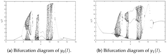
Figure 6. Bifurcation diagrams of system (2) about $\nu$ with $(y_0\left(0\right),y_1\left(0\right))=(1,1),$ $0.01\le \nu \le 15.01$.

It is obvious that the amount of released predators (natural enemies) and the impulsive period have a violent impact on the dynamical property of the system, according to the Figure 3 and Figure 6. Therefore, the impulsive period and the number of released natural enemies should be chosen prudently so that the system can realize an ideal state, which is expected by people.

6. Conclusions

In this article, we propose a predator–prey model with fear factor and impulsive nonlinear effects. This approach is based on the practical consideration of determining pesticide application methods according to an existing pest population, as well as accounting for the influence of fear on prey reproduction. The globally asymptotically stable conditions of the pest-extinction periodic solution $(0,\overline{y_1^{*}\left(l\right)})$ and the permanent condition of the investigated system are derived in accordance with the Floquet theory and the comparison theorem of differential equations. Meanwhile, we also give some simulations to verify our theoretical results. Moreover, we study the more complicated dynamical behaviors of the investigated system, too. Our results indicate that there exists an optimal impulsive period for successful pest management. Furthermore, the impulsive period and amount of released predators will dramatically change the dynamical behaviors of the investigated system. Therefore, we conclude that an appropriate impulsive control period and amount of released predators (natural enemy) should be determined because different parameters cause different scale outbreaks of pests. These outcomes help us design appropriate control strategies and assist us in management decision-making.

Without a doubt, some interesting issues should be considered by us. For instance, what dynamic behaviors will be generated in a system if we consider pest resistance to pesticides due to long-term usage of pesticides? What dynamical behaviors will happen if we think that a pest has a stage structure? These problems will be addressed in our future work.

References

- Savary, S.; Willocquet, L.; Pethybridge, S.J.; Esker, P.; McRoberts, N.; Nelson, A. The global burden of pathogens and pests on major food crops. Nat. Ecol. Evol. 2019, 3, 430–439. [Google Scholar] [CrossRef] [PubMed]
- Zalucki, M.P.; Shabbir, A.; Silva, R.; Adamson, D.; Shu-Sheng, L.; Furlong, M.J. Estimating the economic cost of one of the world’s major insect pests, Plutella xylostella (Lepidoptera: Plutellidae): Just how long is a piece of string? J. Econ. Entomol. 2012, 105, 1115–1129. [Google Scholar] [CrossRef]
- Sogawa, K. Planthopper outbreaks in different paddy ecosystems in Asia: Man-made hopper plagues that threatened the green revolution in rice. In Rice Planthoppers: Ecology, Management, Socio Economics and Policy; Springer: Berlin/Heidelberg, Germany, 2015; pp. 33–63. [Google Scholar]
- Chakravarthy, A.K.; Doddabasappa, B.; Shashank, P.R. The potential impacts of climate change on insect pests in cultivated ecosystems: An Indian perspective. In Knowledge Systems of Societies for Adaptation and Mitigation of Impacts of Climate Change; Springer: Berlin/Heidelberg, Germany, 2013; pp. 143–162. [Google Scholar]
- Liu, Y.H.; Kang, Z.W.; Guo, Y.; Zhu, G.S.; Rahman Shah, M.M.; Song, Y.; Fan, Y.L.; Jing, X.; Liu, T.X. Nitrogen hurdle of host alternation for a polyphagous aphid and the associated changes of endosymbionts. Sci. Rep. 2016, 6, 24781. [Google Scholar] [CrossRef]
- Ali, M.P.; Bari, M.N.; Haque, S.S.; Kabir, M.M.M.; Afrin, S.; Nowrin, F.; Islam, M.S.; Landis, D.A. Establishing next-generation pest control services in rice fields: Eco-agriculture. Sci. Rep. 2019, 9, 10180. [Google Scholar] [CrossRef]
- Heong, K.L.; Wong, L.; Delos Reyes, J.H. Addressing planthopper threats to Asian rice farming and food security: Fixing insecticide misuse. In Rice Planthoppers: Ecology, Management, Socio Economics and Policy; Springer: Berlin/Heidelberg, Germany, 2015; pp. 65–76. [Google Scholar]
- Oerke, E.C. Crop losses to pests. J. Agric. Sci. 2006, 144, 31–43. [Google Scholar] [CrossRef]
- Baker, B.P.; Green, T.A.; Loker, A.J. Biological control and integrated pest management in organic and conventional systems. Biol. Control 2020, 140, 104095. [Google Scholar] [CrossRef]
- Suckling, D.M.; Stringer, L.D.; Stephens, A.E.; Woods, B.; Williams, D.G.; Baker, G.; El-Sayed, A.M. From integrated pest management to integrated pest eradication: Technologies and future needs. Pest Manag. Sci. 2014, 70, 179–189. [Google Scholar] [CrossRef] [PubMed]
- Alharbi, W.; Sandhu, S.K.; Areshi, M.; Alotaibi, A.; Alfaidi, M.; Al-Qadhi, G.; Morozov, A.Y. Revisiting implementation of multiple natural enemies in pest management. Sci. Rep. 2022, 12, 15023. [Google Scholar] [CrossRef]
- Jiao, J.; Chen, L.; Luo, G. An appropriate pest management SI model with biological and chemical control concern. Appl. Math. Comput. 2008, 196, 285–293. [Google Scholar] [CrossRef]
- Dai, X.; Quan, Q.; Jiao, J. Modelling and analysis of periodic impulsive releases of the Nilaparvata lugens infected with wStri-Wolbachia. J. Biol. Dyn. 2023, 17, 2287077. [Google Scholar] [CrossRef]
- Sun, K.; Zhang, T.; Tian, Y. Dynamics analysis and control optimization of a pest management predator–prey model with an integrated control strategy. Appl. Math. Comput. 2017, 292, 253–271. [Google Scholar] [CrossRef]
- Liu, B.; Zhang, Y.; Chen, L. The dynamical behaviors of a Lotka–Volterra predator–prey model concerning integrated pest management. Nonlinear Anal. Real World Appl. 2005, 6, 227–243. [Google Scholar] [CrossRef]
- Guo, H.; Chen, L. A study on time-limited control of single-pest with stage-structure. Appl. Math. Comput. 2010, 217, 677–684. [Google Scholar] [CrossRef]
- Tang, S.; Cheke, R.A.; Xiao, Y. Effects of predator and prey dispersal on success or failure of biological control. Bull. Math. Biol. 2009, 71, 2025–2047. [Google Scholar] [CrossRef]
- Tian, Y.; Tang, S.; Cheke, R.A. Dynamic complexity of a predator-prey model for IPM with nonlinear impulsive control incorporating a regulatory factor for predator releases. Math. Model. Anal. 2019, 24, 134–154. [Google Scholar]
- Dai, X.; Jiao, J.; Quan, Q.; Zhou, A. Dynamics of a predator–prey system with sublethal effects of pesticides on pests and natural enemies. Int. J. Biomath. 2024, 17, 2350007. [Google Scholar] [CrossRef]
- Zhang, Q.; Tang, S.; Zou, X. Rich dynamics of a predator-prey system with state-dependent impulsive controls switching between two means. J. Differ. Equ. 2023, 364, 336–377. [Google Scholar] [CrossRef]
- Liu, X.; Chen, L. Complex dynamics of Holling type II Lotka–Volterra predator–prey system with impulsive perturbations on the predator. Chaos Solitons Fractals 2003, 16, 311–320. [Google Scholar] [CrossRef]
- Zhang, H.; Georgescu, P.; Chen, L. On the impulsive controllability and bifurcation of a predator–pest model of IPM. BioSystems 2008, 93, 151–171. [Google Scholar] [CrossRef]
- Pal, D.; Kesh, D.; Mukherjee, D. Cross-diffusion mediated spatiotemporal patterns in a predator–prey system with hunting cooperation and fear effect. Math. Comput. Simul. 2024, 220, 128–147. [Google Scholar] [CrossRef]
- Mukherjee, D. Role of fear in predator–prey system with intraspecific competition. Math. Comput. Simul. 2020, 177, 263–275. [Google Scholar] [CrossRef]
- Mondal, S.; Samanta, G.P. Impact of fear on a predator–prey system with prey-dependent search rate in deterministic and stochastic environment. Nonlinear Dyn. 2021, 104, 2931–2959. [Google Scholar] [CrossRef]
- Das, B.K.; Sahoo, D.; Samanta, G.P. Impact of fear in a delay-induced predator–prey system with intraspecific competition within predator species. Math. Comput. Simul. 2022, 191, 134–156. [Google Scholar] [CrossRef]
- Zanette, L.Y.; White, A.F.; Allen, M.C.; Clinchy, M. Perceived predation risk reduces the number of offspring songbirds produce per year. Science 2011, 334, 1398–1401. [Google Scholar] [CrossRef]
- Elliott, K.H.; Betini, G.S.; Norris, D.R. Fear creates an Allee effect: Experimental evidence from seasonal populations. Proc. R. Soc. B Biol. Sci. 2017, 284, 20170878. [Google Scholar] [CrossRef]
- Lakshmikantham, V.; Simeonov, P.S. Theory of Impulsive Differential Equations; World Scientific: Singapore, 1989; Volume 6. [Google Scholar]
- Bainov, D.; Simeonov, P. Impulsive Differential Equations: Periodic Solutions and Applications; Routledge: Abingdon, UK, 2017. [Google Scholar]
Disclaimer/Publisher’s Note: The statements, opinions and data contained in all publications are solely those of the individual author(s) and contributor(s) and not of MDPI and/or the editor(s). MDPI and/or the editor(s) disclaim responsibility for any injury to people or property resulting from any ideas, methods, instructions or products referred to in the content. |
© 2025 by the authors. Licensee MDPI, Basel, Switzerland. This article is an open access article distributed under the terms and conditions of the Creative Commons Attribution (CC BY) license (https://creativecommons.org/licenses/by/4.0/).