Abstract
It is a famous hypothesis that orbifold D-brane charges in string theory can be classified in twisted equivariant K-theory. Recently, it is believed that the hypothesis has a non-trivial lift to M-branes classified in twisted real equivariant 4-Cohomotopy. Quasi-elliptic cohomology, which is defined as an equivariant cohomology of a cyclification of orbifolds, potentially interpolates the two statements, by approximating equivariant 4-Cohomotopy classified by 4-sphere orbifolds. In this paper we compute Real and complex quasi-elliptic cohomology theories of 4-spheres under the action by some finite subgroups that are the most interesting isotropy groups where the M5-branes may sit. The computation connects the M-brane charges in the presence of discrete symmetries to Real quasi-elliptic cohomology theories, and those with the symmetry omitted to complex quasi-elliptic cohomology theories.
MSC:
55N34; 81T30; 19L50
1. Introduction
String theory and homotopy theory are closely related. It is a famous hypothesis that orbifold D-brane charges in string theory can be classified in twisted equivariant K-theory, or rather, Real twisted equivariant K-theory. A natural question is whether we have a classification for M-branes in term of cocycles in a generalized cohomology theory.
M-branes are membranes in M-theory, which is a theoretical framework in physics that unifies the five superstring theories and 11-dimensional supergravity. M-branes come in two types, M2-branes and M5-branes. These branes are analogous to the D-branes in string theory but exist in the 11-dimensional spacetime and M-theory. An M2-brane acts as a source for the 3-form field, similar to how an electric charge is a source for the electromagnetic field. In lower dimensions, M2-brane charges can manifest as various types of charges in string theory, such as D2-brane charges or fundamental string charges. In addition, M5-brane is a magnetic dual to the M2-brane and couples to the 6-form field. In string theory, M5-brane charge can appear as NS5-brane charge or D4-brane charge after compactification. M-brane charges play a crucial role in the duality web of string theory and M-theory. They play a key role in unifying string theories, understanding black hole entropy, and studying gauge theories.
A key open problem in M-theory is the identification of the degrees of freedom that are expected to be hidden at ADE-singularities in spacetime. Comparison with the classification of D-branes by K-theories suggests that the answer must come from the right choice of generalized cohomology theory for M-branes. Recently it is believed that the hypothesis has a non-trivial lift to M-branes classified in twisted real equivariant 4-Cohomotopy. Then, it is an evident question how the statement for D-branes and this for M-branes may relate.
As indicated in [1], cyclification of ∞-stacks is a fundamental and elementary base-change construction over moduli stacks in cohesive higher topos theory. Quasi-elliptic cohomology theory, which is defined as an equivariant cohomology of a cyclification of orbifolds, is a form of twisted equivariant K-theory involving a further -action, just as one would expect in lifting through the M/II reduction. It is a variant of Tate K-theory. Quasi-elliptic cohomology theory is a generalized cohomology theory that potentially interpolates the two statements, by approximating equivariant 4-Cohomotopy classified by 4-sphere orbifolds. In addition, the universal shifted integral 4-class of equivariant 4-Cohomotopy theory on ADE-orbifolds induces the Platonic 4-twist of ADE-equivariant Tate-elliptic cohomology,
In [2], the author computes a list of examples explicitly, specifically for the domain being orbifolds of 4-spheres by finite subgroups of that serve as the transverse geometry to M5-branes probing ADE-singularities. The results in all cases investigated are deformations of familiar twisted equivariant K-theory groups by a further formal variable q, being the character of the extra -action and playing the role of a kind of M-theoretic quantum deformation of the K-theory groups.
In this paper, we consider the approximation of the Real version of quasi-elliptic cohomology to Real twisted equivariant 4-Cohomotopy. Young and the author construct a Real version of quasi-elliptic cohomology in [3]. Since twisted equivariant -theory appears in physical contexts that are unoriented, such as orientifold string theory [4] and unoriented topological field theory [5,6], it is natural to expect a relation between unoriented conformal field theory and a Real generalization of elliptic cohomology. This expectation suggests the promotion of the group of loop rotations to the orthogonal group so as to include loop reflection, an orientation reversing symmetry of loops. The -equivariant topology of loop spaces has been studied by a number of authors [7,8,9,10,11]. In [3], Real quasi-elliptic cohomology is constructed as the -equivariant Freed–Moore K-theory of an inertia groupoid. In this paper, we compute Real and complex quasi-elliptic cohomology of 4-spheres under the specific action of some finite subgroups of , which aims to give an approximation to the Real equivariant unstable 4th Cohomotopy, which is especially difficult to compute.
To interpret the relation between the computation and cohomotopy, we start the story by classifying spaces for cohomology theories. For a given cohomology theory with classifying space E, we have, for any good enough space X,
Here, we can regard a map as a “cocycle” for the E-cohomology, and a homotopy between such maps as a “boundary” in E-cohomology. Generally, the classifying space of an abelian cohomology theory is its spectrum at level 0. A classical example is complex topological K-theory , whose classifying space can be taken to be .
In addition, instead of using the whole spectrum of E, with only the classifying space, we can define a generalized non-abelian cohomology theory
which makes good sense. One issue is that computing such cohomology theories is generally difficult. One method is approximating the cohomology theory E by another one , which is better understood and easier to compute. The method is clearly possible whenever there is a map of classifying spaces because it induces, evidently, a cohomology operation
which provides an image of the less-understood E-cohomology in the better-understood -cohomology.
The archetypical example here is the Chern-Dold character map [12,13], which approximates any generalized cohomology theory by a rational cohomology theory. For instance, the ordinary Chern character on
with is represented by a map of classifying spaces
This map of classifying spaces is itself a cocycle in the rational cohomology of the classifying space . In other words, the Chern character itself can be viewed as an element in
Generally, a map of classifying spaces , inducing a cohomology operation , is itself a cocycle in the -cohomology of the classifying space E. Thus, in order to understand E-cohomology, we may try to understand the -cohomology of its classifying space E for suitable alternative cohomology theories .
Now, we consider the cohomology theory, the n-th Cohomotopy theory
whose classifying space is an n-sphere . Each cocycle in the -cohomology is represented by a map . From it, we obtain a cohomology operation
which provides us images of in -cohomology similarly to how the Chern character provides images of K-cohomology in ordinary rational cohomology.
It is suggested by Hypothesis H [14,15,16] that, specifically, -twisted equivariant unstable 4 classifies the charges carried by M-branes in M-theory in a way that is analogous to the traditional idea that classifies the charges of D-branes in string theory. Therefore, it is essential to compute the of spacetime domains relevant in M-theory. This can be hard, in particular, once we remember that all of these need to be performed in twisted equivariant generality. Thus, we apply the idea to approximate of spacetime by using the cocycles
in for some suitable cohomology theory . Instead of itself, we will study the image of the corresponding cohomology operation
Some information of the actual may be lost but what is retained can still be valuable and is expected to be better understandable.
Specifically, the classifying spaces for equivariant are orbifolds of the 4-sphere acted by a group G, i.e., the orbifolds of representation 4-spheres. Hence, the elements of the G-equivariant -cohomology serve, in the above way, as “generalized equivariant characters” on equivariant , namely, as the equivariant cohomology operation
As conjectured in [1], the choice
should be a particularly suitable approximation to equivariant for the purpose of computing M-brane charge. One motivation for this is that the Witten elliptic genus, which was originally discussed for string [17], actually makes sense for M5-branes [18,19,20,21,22], so that one should expect that it is actually part of the charges carried by M5-branes. But these charges should also be in , and hence, it is conjectured in [1] that there is a useful approximation of by elliptic cohomology, and specifically by quasi-elliptic cohomology.
This is the motivation for computing the quasi-elliptic cohomology for representation 4-spheres. Moreover, as indicated in [13], the particular choice of equivariance groups G as finite subgroups of comes from the fact that these are the most interesting isotropy groups for the orbifolds on which these M5-branes may sit. We describe the interesting groups and their action on 4-spheres below.
The space of quaternions is isomorphic to as a real vector space. In addition, the group of the unit quaternions is isomorphic to the special unitary group , which is isomorphic to . It can be identified with a subgroup of via the composition
where the first homomorphism is the inclusion into the first factor. Under quaternion multiplication, there are two choices of group action by on that we are especially interested in.
The group action can extend to by keeping the north pole and the south pole fixed. In ([2] Section 6), we compute complex quasi-elliptic cohomology of under the first group action in (1). In Section 4, we compute the Real quasi-elliptic cohomology for that. Moreover, in Section 5, we compute some examples of complex and Real quasi-elliptic cohomology of under the second group action in (1). In addition, in Section 6.1, we discuss the relation between the computation and physics a little; in Section 6.2, we give a future problem that we are interested in.
In the computation of Real quasi-elliptic cohomology theories, we pick a Real structure on each equivariance group, with which the corresponding theories are computable. Real quasi-elliptic cohomology is defined as a Freed–Moore K-theory of a Real version of an inertia groupoid. The computation in Section 4 shows how the classification of M-brane charges is described by equivariant complex K-theories when the conjugacy classes are free under the involution, and how the classification is described by equivariant KR-theories when the conjugacy classes are fixed by the involution. In Section 5.2, we compute some Real and complex quasi-elliptic cohomology theories whose equivariance groups are some finite product subgroups of . The conjugacy classes of the equivariance group determine the distinct types of localized charges, while the Real conjugacy classes describe how these charges behave under the involution. The connection is formalized using equivariant K-theories and equivariant KR-theories, which provide a deep link between geometry, algebraic topology and physics.
In addition, we would like to mention some other methods approximating 4-Cohomotopy, which is a challenging task in equivariant homotopy theory. Generally, a G-equivariant 4-Cohomotopy of a space X is difficult to compute and depends heavily on the equivariance group G and the topological space X. Tools from equivariant homotopy theory, such as the Borel construction, equivariant cohomology, and spectral sequences, are often used to study these groups. We list a few of them below.
- (1)
- One method is to use obstruction theory to determine whether a G-equivariant map exists and classify such maps up to homotopy [23]. This method works well for spaces that can be decomposed into G-CW complexes. However, obstruction classes can be difficult to compute explicitly, especially for higher dimensional spaces.
- (2)
- In addition, we can apply Atiyah–Hirzebruch spectral sequence or the Serre spectral sequence to approximate equivariant 4-Cohomotopy whose -page involves terms like [24]. This method breaks down the problem into simpler pieces using cohomology and homotopy groups. It can handle a wide range of spaces X and equivariance groups G. But higher differentials in the spectral sequence are often difficult to compute and the spectral sequences may not always converge cleanly.
- (3)
- Another method is that we stabilize the problem first by replacing with its stabilization and use equivariant Adams spectral sequence to approximate 4-Cohomotopy [24]. Reducing the problem to stable homotoy groups certainly simplifies the problem and Adams spectral sequence is a powerful tool. However, stabilization loses some geometric information about X and the 4-sphere, and the unstable problem of interest may not directly be solved.
- (4)
- In addition, when the space X has a smooth structure and the G-action is geometric, one can study G-equivariant instantons or harmonic maps to [25,26]. Using these methods, the equivariant maps can be constructed explicitly, which may connect to physical applications. But the method may not be generalized to more abstract or singular spaces.
The method we use in this paper is a novel one. It works well especially when the cohomology theory approximating 4-Cohomotopy is suitably chosen and computable. In this paper, we implemented this idea.
In the Appendix A and Appendix B, we give some corollaries of the decomposition formula for complex equivariant K-theories in [27] and the Mackey decomposition formula for Freed–Moore K-theories in [3]. They are used in the computation in Section 4 and Section 5, respectively.
2. Quasi-Elliptic Cohomology
In this section, we recall the definition of quasi-elliptic cohomology in term of equivariant K-theories and state the conclusions that we need in this paper. For more details on quasi-elliptic cohomology, please refer to [28].
Let G be a compact Lie group and X a G-space. Let denote the set of torsion elements of G. For any , the fixed point space is a space where is the centralizer . This group action can be extended to that by the group
which is given explicitly by
for any and .
The inertia orbifold of is defined to be the functor groupoid
The inertia orbifold plays an import role in the geometry and index theory of orbifolds [29,30]. The rotation action of the circle group can be built into it as new morphisms, as we see in Definition 2.
To give a complete description of the loop groupoid , we need the following definitions.
Definition 1.
(1) Let g, be two elements in G. Define to be the set (2) Let denote the quotient of under the equivalence
where l is the order of g in G.
Definition 2.
Define to be the groupoid with
- objects: the space
- morphisms: the space
For an object , the morphism is an arrow from x to The composition of the morphisms is defined by
Let denote the circle group . We have a homomorphism of orbifolds
sending all the objects to the single object in , and a morphism to in .
Definition 3.
The quasi-elliptic cohomology is defined to be .
The groupoid is equivalent to the disjoint union of action groupoids
where is the conjugation quotient groupoid. Thus, we can unravel Definition 3 and express it via equivariant K-theory.
Definition 4
([28] Definition 3.11).
Consider the composition
where is the projection and the second map is defined via the collapsing map . Via it, is naturally a algebra.
Proposition 1
([28] (1.1)). The relation between quasi-elliptic cohomology and equivariant Tate K-theory is
This is the main reason why the theory is called quasi-elliptic cohomology.
In addition, we give an example computing quasi-elliptic cohomology, which is ([28] Example 3.3). The conclusions in Example 1 are applied in the computation of Section 4 and Section 5.
Example 1
(). Let for , and let . Given an integer which projects to , let denote the representation of defined by
is isomorphic to the ring .
3. Twisted Real Quasi-Elliptic Cohomology
In this section, we review the definition and properties of twisted Real quasi-elliptic cohomology. For more details, please refer to [3].
We will use -graded groups to define the Real structure on groups.
Definition 5.
Let G be a finite group. A is a group homomorphism . The ungraded group of is . When π is non-trivial, is called a Real structure on G. The group acts on G by Real conjugation
. The Real centralizer of is
The group is -graded with ungraded group the centralizer .
Example 2.
The terminal -graded group is and is denoted simply by . If acts on a group , then so does any -graded group and the resulting semi-direct product is naturally -graded.
Example 3.
The dihedral group
is a Real structure on . The subgroup is a normal subgroup of and we have the short exact sequence
with a generator of mapped to the rotation r.
Example 4.
As computed in ([3] Example 1.8), the Real representation ring with respect to the Real structure is isomorphic to complex representation ring
Example 5.
For any , the Real centralizer is -graded with ungraded group the centralizer . It is a Real Structure on .
In addition, the element is Real central and so generates a normal subgroup isomorphic to . This leads to the definition of the enhanced Real centralizer of g.
It is a Real structure on the group .
The set of connected components of the conjugation quotient groupoid is the set of conjugacy classes of G. Given a Real structure , Real conjugation defines an involution of . This defines a partition
with the fixed point set of the involution. The conjugacy class of is fixed by the involution if and only if . The set of Real conjugacy classes of G inherits from (8) a partition
Let X be a -space. Note that for each , the fixed point space is a -space. In addition, the -action on as defined in (2) can extend to an action by :
for any element , any .
The Real loop groupoid , as defined in ([3] Definition 2.7), adds the involution as morphisms into the groupoid , and it is a double cover of the groupoid . In addition, we have the Real version of the decomposition (4), i.e., the decomposition of the groupoid corresponding to the partition (9).
Proposition 2.
There is an equivalence of -graded groupoids
The twisted Real quasi-elliptic cohomology is defined in ([3] Definition 3.2, Proposition 3.3) in terms of Freed–Moore K-theories.
Definition 6
([3] Definition 3.2 Proposition 3.3).
where is a fixed element in and is the Real transgression map.
By the property of the Freed–Moore K-theory [5], if the Real structure splits, each factor in (12) is the equivariant -theory defined by Atiyah and Segal [31].
The -graded morphism which tracks loop rotation and reflection makes into a -algebra and, in particular, a module over .
Theorem 1
([3] Theorem 3.15). Assume that is non-trivially -graded. The relation between twisted Real quasi-elliptic cohomology and twisted Real equivariant Tate K-theory is
In addition, we give an example computing Real quasi-elliptic cohomology, which is ([3] Example 3.7). The conclusions in Example 6 are applied in the computation of Section 4 and Section 5.
Example 6.
4. Real Quasi-Elliptic Cohomology of Acted by a Finite Subgroup of Spin(3)
In this section, we compute all the Real quasi-elliptic cohomology theories
where G goes over all the finite subgroups of .
First, we explain how the group G acts on . We have the standard orthogonal -action on and also on the subspace . The covering map
makes a well-defined -space. The G-action on is induced by the composition
where is the projection to the first factor of the product group.
We give the explicit formula of the G-action below. The group of unit quaternions is isomorphic to via the correspondence
In view of this, can be described as the group
and can be identified with the quaternionic unitary group. Thus, as indicated in ([32] p. 263), the inclusion from is given by the formula
In addition, as shown in ([32] p. 151), the rotation of represented by
is given by the map
where is identified with the linear space
Then, the group acts on via the composition
and the standard orthogonal action.
In the rest part of the paper, we will use the symbol
to denote the matrix
and the symbol
to denote the matrix
First, we need to pick a Real structure on the group as well as on all its finite subgroups by equipping the group with a reflection s. The choice is definitely not unique. Next, we define the reflection action on and, thus, together with (18), we define the action on by .
Example 7.
Motivated by the Real structure
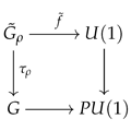
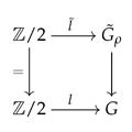
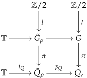
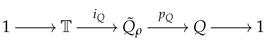
of the cyclic group , we want to pick a Real structure on making the diagrams below commute.
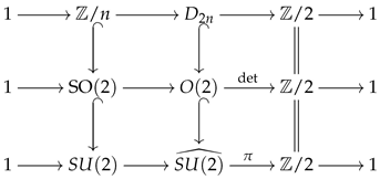 where the horizontal sequences are all exact. In the left column, the generator r of the rotation group is mapped to the rotation in . The lower left vertical map can be chosen to map the rotation to . In addition, the reflection in can be mapped to
It is straightforward to check that is the identity map for any θ.
where the horizontal sequences are all exact. In the left column, the generator r of the rotation group is mapped to the rotation in . The lower left vertical map can be chosen to map the rotation to . In addition, the reflection in can be mapped to
It is straightforward to check that is the identity map for any θ.
In addition, we can take the action of s on to be
Note that under the reflection (21), the north and south poles of are still fixed. On the -plane, the two pairs of points
are switched by the reflection, respectively. It is straightforward to check that acts as the identity map on for any θ. Thus, it is reasonable to take the Real structure to be the subgroup
of and take the projection to be the determinant map det.
Instead, we can map the rotation r to the matrix , which is a conjugation of . We have
where and θ is any real number. In addition, the reflection s is fixed under the conjugation. The corresponding Real structure of is still and the diagram (20) still commutes.
Moreover, we would like to mention a different choice of the Real structure . In the diagram (20), we map the rotation in to the same matrix in but map the reflection to
Note that , i.e., is not a fixed point under the conjugation taking to . We can check, for any θ, . The action of on can be defined as
Under the reflection (22), the north and south poles are also fixed. On , the two pairs of points
are switched by the reflection, respectively. It is straightforward to check that acts as identity on for any θ. Thus, it is reasonable to take the Real structure to be the subgroup
of and the projection π to be the determinant det.
Since is a normal subgroup of , both Real structures, and , split.
Example 8.
For any finite subgroup G of ,
is the restriction of the Real structure
of to G. It defines a Real structure on G.
Similarly,
defines a Real structure on G.
Remark 1.
We give in Example 7 some reasonable choices of reflection on the representation sphere , which all keep the north pole and the south pole fixed. We did not find a canonical choice of reflection that switches the north pole and the south pole.
As indicated in ([33] p. 215), for V, a real vector space equipped with a linear G-action, stereographic projection exhibits a G-equivariant homeomorphism between the representation sphere (the one-point compactification) and the unit sphere (where the -summand is equipped with the trivial G-action):
Another reasonable choice of the reflection on is the one sending a point to . The map corresponding to that on , which is
where is the length of the vector. The map preserves the angle but not the length of the vector when it is not 1, and, especially, it is not linear. Thus, this is not the right choice of reflection for our computation.
Remark 2.
We would like to mention that, other than the choice of the Real structure, the choice of the action of on is also not unique where G is any finite subgroup of . Though different choices of the Real structure may lead to different , different choices of the action of the reflection may lead to little difference.
In the computation of with G a finite subgroup of , for most elements , the fixed point spaces consist of only the north pole and the south pole, where the reflections, those in Example 7, etc., act trivially. In addition, for the identity element , is a representation sphere of the group . Thus, by ([34] Theorem 5.1), the computation of the corresponding factor can be reduced to that of the Real representation ring of .
To compute the Real quasi-elliptic cohomology of 4-spheres
acted by a finite subgroup
we need to find all the fixed points in G under the involution, i.e., the Real conjugation. Below is a conclusion that we will apply in the computation later.
Proposition 3.
If we take the Real structure on a finite subgroup G of , for any element β in G, we have the conclusions below.
- (1)
- The element β is a fixed point under the involution if and only if is in the conjugacy class of β in G.
- (2)
- If β is a unit quaternion whose coefficient of i is zero, then and β is a fixed point under the involution.
Proof.
A given element is a fixed point under the involution if and only if the set is nonempty, i.e., there is an element for some satisfying
So we obtain the first conclusion.
Since is an element in , thus, it has a quaternion representation . In (ii), we discuss a very special case that . We start the computation below.
The right hand side should be the inverse of . So we establish the equation
Solving the equation, we obtain
i.e.,
if and only if is a unit quaternion with . □
Similarly, we have the conclusion.
Proposition 4.
If we take the Real structure on a finite subgroup G of , for any element β in G, we have the conclusions below.
- (1)
- The element β is a fixed point under the involution s if and only if is in the conjugacy class of β in G.
- (2)
- If β is a unit quaternion whose coefficient of k is zero, then we have and β is a fixed point under the involution.
The proof is analogous to that of Proposition 3.
Next, we will compute with G a finite subgroup of one by one. Before that, we recall the classification of the finite subgroups of . There are many references for the classification, including ([35] Chapter XIII), [36,37] etc. The finite subgroups of are classified as follows:
- the cyclic group of order n
- the dicyclic group of order
- the binary tetrahedral group ;
- the binary octahedral group ;
- the binary icosahedral group ;
where n is any positive integer.
Example 9.
In this example, we compute where is the finite cyclic subgroup
We take the Real structure as defined in Example 8, i.e., the group below together with the determinant map det
It is isomorphic to the dihedral group . The involution on is trivial.
Thus, by ([3] Example 3.7), we obtain directly that
where consists of the fixed points, i.e., the south pole and the north pole of . Thus,
and by ([3] Example 3.7), the right hand side is isomorphic to
In addition, by ([34] Theorem 5.1),
In conclusion,
Example 10.
In this example, we compute where is the dicyclic group
where τ is the reflection
The Real structure on is taken to be , as that defined in Example 8.
In , there are conjugacy classes. They are as follows:
- (1)
- ,
- (2)
- ,
- (3)
- , , ⋯, ,
- (4)
- ,
- (5)
- ,
where the first two classes form the centre of the group.
By Proposition 4, all the conjugacy classes are fixed points under the reflection s. Thus, all the factors in are equivariant KR-theories. The factor in corresponding to each conjugacy class is computed below one by one.
- (1)
- First, we consider the Real conjugacy class represented by I. The centralizer and the Real centralizer isThen, the group By ([34] Theorem 5.1),Note that is a Real structure on .
- (2)
- Then, we consider the Real conjugacy class represented by . In this case, the centralizer and the Real centralizerIn this case, we have the Real central extensionBy Corollary A1,where is the sign representation of .
- (3)
- Then, we compute the factor in corresponding to which is not .The centralizer is the cyclic group ; and the Real centralizeris the dihedral group of order . In this case, by ([3] Example 3.7),
- (4)
- Then, we compute the factor corresponding to the conjugacy class represented by τ. The centralizer and the Real centralizerThus,
- (5)
- For the conjugacy class represented by , the centralizer and the Real centralizer . Then, the factor corresponding to is
In conclusion,
where is the sign representation of .
Example 11.
In this example, we compute where is the binary tetrahedral group . We take the Real structure on it, i.e.,
The quaternion representation of is given explicitly in [38,39].
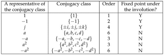
We can compute the conjugacy classes in explicitly. A multiplication table for the binary tetrahedral group is given in [40]. For the convenience of the readers, we apply the same symbols of the elements as those in [39,40]. A list of representatives are given in Figure 1. This list can be obtained by direct computation. In addition, by Proposition 3, an element in represents a fixed point in if and only if it is , , or . Note that, for , if we take the Real structure , we will obtain the same set of fixed points under the reflection.
Figure 1.
Conjugacy classes of .
Below, we compute the factors of corresponding to each conjugacy class respectively.
- (1)
- For the conjugacy class represented by I, the Real centralizer . By ([34] Theorem 5.1), we have
- (2)
- For the conjugacy class represented by , we have .Let denote the group . We have the short exact sequenceEspecially, we have the commutative diagram below:
 Note that we have the short exact sequenceBy Corollary A1,where is the sign representation of .
 - (3)
- For the conjugacy class represented by j, . The centralizer and the Real centralizerThus,
- (4)
- For the conjugacy class represented by a, we have
- (5)
- For the conjugacy class represented by , we have
- (6)
- For the conjugacy class represented by , we have
- (7)
- For the conjugacy class represented by , we have
Thus, in conclusion,
where is the sign representation of .
Example 12.
In this example, we compute where is the binary octahedral group. We take the Real structure on it, i.e., .
A presentation of is given as
We can obtain immediately that . Equivalently, there is a quaternion presentation of given by the embedding
sending θ to , t to , and r to .
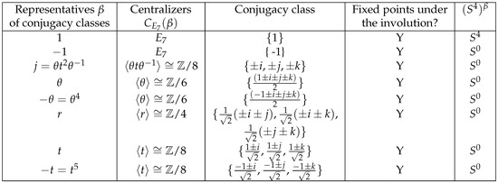
By [41] and direct computation, we obtain Figure 2, which provides a list of the representatives of the conjugacy classes of , the centralizers of each representative, and the corresponding fixed point spaces.
Figure 2.
Conjugacy classes, centralizers, and fixed point spaces.
Below, we give the factor of corresponding to each conjugacy class.
- (1)
- For the conjugacy class represented by I, the Real centralizer . The factor corresponding to I
- (2)
- For the conjugacy class represented by , the Real centralizer . Let denote the chiral octahedral group and the Real structure , and we have the commutative diagram below.
 Thus, by Corollary A1,where is the sign representation of .
 - (3)
- For the conjugacy class represented by j is , its Real centralizerThus, is isomorphic to
- (4)
- For the conjugacy class represented by , the Real centralizerNote that and . Then is isomorphic to
- (5)
- For the conjugacy class represented , the Real centralizerThen, is isomorphic to
- (6)
- For the conjugacy class represented by , the Real centralizerThus, is isomorphic to
- (7)
- For the conjugacy class represented by , its Real centralizerThus, is isomorphic to
- (8)
- For the conjugacy class represented by , its Real centralizerThus, is isomorphic to
Thus, in conclusion,
where is the sign representation of .
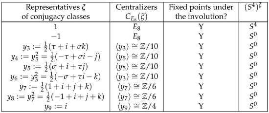
Example 13.
In this example, we compute where is the binary icosahedral group. A presentation of this group is
The cardinality of is 120. In this example, we use τ to denote and σ to denote the number . We take the Real structure on , i.e., .
By ([42] p. 7635, Table 1) and direct computation, we obtain a list of the representatives of the conjugacy classes of , the centralizers of each representative, whether it is fixed under the involution or not, and the corresponding fixed point spaces in Figure 3.
Figure 3.
Conjugacy classes, centralizers, and fixed point spaces.
Next, we compute each factor of corresponding to each conjugacy class of .
- (1)
- For the conjugacy class , the Real centralizer . Thus, by ([34] Theorem 5.1),
- (2)
- For the conjugacy class , the Real centralizer . Thus, by Corollary A1,where is the sign representation of .
- (3)
- For the conjugacy class represented by , its Real centralizerThus, is isomorphic to
- (4)
- For the conjugacy class represented by , the Real centralizerThus, is isomorphic to
- (5)
- For the conjugacy class represented by , the Real centralizer Thus, the factor is isomorphic to
- (6)
- For the conjugacy class represented by , the Real centralizer Thus, the factor is isomorphic to
- (7)
- For the conjugacy class represented by , the Real centralizer Thus, the factor is isomorphic to
- (8)
- For the conjugacy class represented by , the Real centralizer Thus, the factor is isomorphic to
- (9)
- For the conjugacy class represented by , the Real centralizerThus, the corresponding factor is isomorphic to
In conclusion,
where is the sign representation of .
Remark 3.
As we can see in the examples of this section, most computations lead to the equivariant KR-theory of a single point. The whole data of the equivariant KR-theory, by the computation in ([31] Section 8) and ([43] Proposition 3.1), are given as
where and are the forgetful functors, the map ρ is given explicitly in ([43] Proposition 2.17), and the map η is given explicitly in ([43] Proposition 2.24).
In addition, there is a graded ring isomorphism (see [31] Section 8)
5. Quasi-Elliptic Cohomology of Acted by a Finite Subgroup of Spin(4)
In this section, we compute with G a finite subgroup of . The -action on that we are interested in is that given by the Formulas (18) and (19).
Denote by the space of quaternions, to be regarded mainly as a real module under quaternion multiplication from the left and right, in particular by unit quaternions
We have group isomorphism
and
under which the spin double cover of is given by
5.1. Warm-Up Examples
We start with a simple example.
Example 14.
In ([2] Section 6) and Section 4, we compute complex and Real quasi-elliptic cohomology of under the action of the finite subgroups of . In this example We consider the “dual" of them, i.e., the finite subgroup of , which are the groups
For a point , it acts on a point by
For any finite subgroup G of , for any torsion point , ; and the centralizer . Thus, . For the Real case, the Real centralizer It is straightforward to check case by case that
and the Real quasi-elliptic cohomology
Example 15.
In this example, we study the -action on induced by the involution x on
The north pole and south pole are both fixed points under the involution.
There are two conjugacy classes in corresponding to its two elements.
Below, we compute the factors of .
- For the conjugacy class 1, is itself. .
- For the conjugacy class τ,
Next we compute . If we take the Real structure on to be the Dihedral Real structure, we can take the reflection to be
The composition sends a point to , i.e., the quaternion conjugation. The group generated by x and y is the dihedral group .
Additionally, the Real centralizers for , τ in . The factors of are computed below.
- For the conjugacy class 1, .
- For the conjugacy class τ,
Next, we compute and with G a cyclic subgroup of .
Example 16.
Let
Let
denote a generator of the cyclic group. We can assume that and are coprime, and and are coprime. The order of G is the least common multiple N of and .
Then, for any , the centralizer
And
The group is isomorphic to . Then, we can apply the results in [2] and Example 9 directly.
The complex quasi-elliptic cohomology is
The Real quasi-elliptic cohomology is
5.2. Product of Finite Subgroups
I did not find all the finite subgroups of that have a well-defined action on . I will discuss some finite subgroups of the form where both H and K are finite subgroups of .
Example 17.
For any , and , as given in (26),
The set of conjugacy classes is a one-to-one correspondent to . In addition,
If is a Real structure on H and is a Real structure on K, then we have the product Real structure
where the projection
sends to . For the Real centralizers,
Thus,
where is the 2-dimensional orthogonal group.
In addition, if the reflection in and on are represented by the same matrix with , it defines a -linear map
Then, by direct computation, if we take α to be the reflection s defined in Example 7, the resulting reflection on is defined by
And if we take α to be the reflection defined in Example 7, the resulting reflection is
In addition, if we take the reflection in to be s and that on to be , the resulting reflection on is
And if we take the reflection in to be and that on to be s, the resulting reflection on is
In fact, we have a conclusion generalizing Example 14.
Proposition 5.
Let H and K denote two finite subgroups of . The product acts on in the way as in (26). Then,
Moreover, if is Real structure on H and is Real structure on K, then,
Proof.
We first notice the factors of both and go through the set .
Then, by (27), for any , and ,
In addition, for any fixed point of , we have the equality
Taking the complex conjugate of both sides, we obtain
Thus, the complex conjugate of the quaternion induces a one-to-one correspondence
Moreover, it is direct to show that for any element , any , we have the equality
Note that . This leads to the isomorphism
Thus,
For the Real case, the factors of both and go through the same set . In addition, by (28),
And the complex conjugate
commutes with the reflections, as shown below.
 where is the reflection in and is the reflection in .
Thus, we obtain
□
Proposition 6.
Let H and K denote two finite subgroups of . The product acts on by the action given in (18). Let denote a Real structure on H and a Real structure on K. Then, we have the conclusions below.
- (1)
- The factor in corresponding to the conjugacy class , i.e., , is isomorphic toThen, we have the isomorphism
- (2)
- The factor in corresponding to the Real conjugacy class , i.e., , is isomorphic to
- if is a fixed point under the involution;
- if is a free point under the involution.
Proof.
We prove the conclusions one by one.
- (1)
- Note that (18) defines a 4-dimensional representation of . Thus, is a representation sphere of and contains as a subspace. Whatever is, by ([34] Theorem 4.3), we haveAnd the right hand side is isomorphic toSo the first conclusion is proved.
- (2)
- The proof is similar to the complex case. Since is both a Real representation sphere of and a complex representation sphere of , thus, by ([34] Theorem 4.3, Theorem 5.1), the Freed–Moore K-theory is isomorphic toIn addition,And .
Then, we obtain the conclusion immediately. □
Remark 4.
One probably subtle point is that, as indicated in [3], the Real structure we takes in the in the general definition of the enhanced Real stabilizer
It is the reflection of . This coincides with the dihedral Real structure on . More explicitly, the involution defined from the dihedral Real structure on is given by , which is the quotient of the reflection on .
The Real representation ring for with the dihedral Real structure, i.e., , is exactly , which is isomorphic to . Thus, the isomorphism
gives us the isomorphism of Real representation rings, i.e.,
Example 18.
In this example we compute with
By ([2] Example 6.3) and Proposition 6(1),
We take the Real structure as defined in Example 8, i.e., the group below together with the determinant map det
It is isomorphic to the dihedral group . As discussed in Example 9, all the elements in and are fixed points under the involution; thus, so are those in .
By Example 9 and Proposition 6(2),
Example 19.
Let n and m be positive integers. Let denote the cyclic group
and denote the binary Dihedral group
In this example, we compute and .
Let τ denote in , which is in terms of quaternions.
The factors of corresponding to each conjugacy class are computed one by one below. We first compute the factors corresponding to the conjugacy classes represented by
- (1)
- If ,where the isomorphism is by ([34] Theorem 4.3).
- (2)
- If the in (29) is not , the centralizer .
- (3)
- If the in (29) is , the centralizer .
- If ,
- If , applying Proposition A1, we obtainwhere ρ is the sign representation of .
- (4)
- For the conjugacy class of , The centralizer
- (5)
- Then, we study the case corresponding to the conjugacy class ofThe centralizer Thus,where the isomorphism is by ([34] Theorem 4.3).
Example 20.
We compute in this example. We take the Real structure and as discussed in Example 8. From them, we formulate a Real structure
on the product . By Example 9, all the elements in are fixed points under the involution; and by Example 10, all the elements in are fixed points under the involution. Thus, all the points in are fixed points.
We compute the factors of below one by one. We start with those corresponding to the conjugacy classes represented by
with k, .
- (1)
- If , by ([34] Theorem 5.1),
- (2)
- If the in α is not ,
- (3)
- If the in α is I,
- (4)
- If the in α is , applying Corollary A1, we getwhere is the sign representation of .
- (5)
- For the conjugacy class of ,
- (6)
- For the conjugacy class of ,
Example 21.
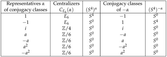
In this example, we deal with the finite subgroup of where is the binary tetrahedral group and is the binary octahedral group, and compute the complex quasi-elliptic cohomology .
First, for the conjugacy classes where α is a conjugacy class in and 1 represents the conjugacy classe consisting of itself in , we have
Note that . The first factor above is the factor in corresponding to the conjugacy class α, which is computed explicitly in ([2] Example 6.5).
For the factors corresponding to the conjugacy classes where β is a conjugacy class in , as we discuss in Example 14, , and
where is the factor of corresponding to the conjugacy class represented by β, which is computed explicitly in ([2] Example 6.6).
Then, we think about the case corresponding to the conjugacy classes of the form . By direct computation,
We provide the conjugacy class of each and each fixed point space in Figure 4, where .
Figure 4.
Centralizers and fixed point spaces of .
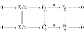
In addition, we have the short exact sequence
Note that the image of is contained in the center of ; thus, we can apply Proposition A1.
For , the action of on is trivial. So, we have
where ρ is the sign representation of . Applying the computation in ([2] Example 6.5, Example 6.6), we list the result of the computation of () below.
| Representatives | The factor |
| of conjugacy classes | |
| 1 | |
| i | |
| a | |
Then, we discuss the case that .
where ρ is the sign representation of .
Next, we deal with the factor corresponding to the conjugacy classes
By direct computation, we can obtain
| Representatives | The fixed point space | |
| of conjugacy classes | is isomorphic to | |
| 1 | ||
| i | ||
| a | ||
For ,
where ρ is the sign representation of .
We list the computation of the other cases () below.
| Representatives | The factor |
| of conjugacy classes | |
| 1 | |
| i | |
| a | |
Next, we deal with the conjugacy classes
and compute the factors .
By direct computation, we can obtain
| 1 | ||
| i | ||
| a | ||
We list the computation of below.
| Representatives | The factor |
| of conjugacy classes | |
| 1 | |
| i | |
| a | |
Next, we deal with the conjugacy classes
By direct computation, we can obtain
| 1 | ||
| i | ||
| a | ||
We list the computation of below.
| Representatives | The factor |
| of conjugacy classes | |
| 1 | |
| i | |
| a | |
Next, we deal with the conjugacy classes
and compute the factors .
By direct computation, we can obtain
| 1 | ||
| i | ||
| a | ||
We list the computation of below.
| Representatives | The factor |
| of conjugacy classes | |
| 1 | |
| i | |
| a | |
Next, we deal with the conjugacy classes
and compute the factors .
By direct computation, we can obtain
| 1 | ||
| i | ||
| a | ||
We list the computation of below.
| Representatives | The factor |
| of conjugacy classes | |
| 1 | |
| i | |
| a | |
Next, we deal with the conjugacy classes
and compute the factors .
By direct computation, we can obtain
| 1 | ||
| i | ||
| a | ||
We list the computation of below.
| Representatives | The factor |
| of conjugacy classes | |
| 1 | |
| i | |
| a | |
Example 22.
In this example, we compute the Real quasi-elliptic cohomology . We take the Real structure of given in Example 11 and the Real structure of given in Example 12. Note that an element is a fixed point under the reflection if and only if h is a fixed point in and k is a fixed point in ; in addition, an element is a free point under the reflection if and only if h is a free point in and k is a free point in .
As shown in Example 12, all the representatives of the conjugacy classes in , as given in Figure 2, are fixed points under the reflection. Thus, all the representatives of the conjugacy classes in are fixed points and they are represented by the elements with h a fixed point. Then, by Figure 1, h can only be 1, and j.
We first deal with the conjugacy classes
where β goes over all the representatives of the conjugacy classes in and compute the factors .
Applying Proposition 6, we list the computation of below.
| Representatives | The factor |
| of conjugacy classes | |
| 1 | |
| j | |
| r | |
| t | |
Next, applying Proposition 6, we list the computation of below.
| Representatives | The factor |
| of conjugacy classes | |
| 1 | |
| j | |
| r | |
| t | |
In addition, we list computation of below.
| Representatives | The factor |
| of conjugacy classes | |
| 1 | |
| j | |
| r | |
| t | |
6. Conclusions and Future Problems
6.1. Relation to Physics
In this section, we sketch the relation between the computation in Section 4 and Section 5 and physics. We would like to leave a more detailed interpretation of the relation to physicists.
The results in Section 4 are the Real analogues of those in [2]. In most cases investigated, the results are deformations of twisted equivariant KR-theory groups or twisted equivariant K-theory groups by a further formal variable q, being the character of the extra -action and playing the role of a kind of M-theoretic quantum deformation of the K-theory groups.
The interesting points lie in the decomposition (9). In the computation of Real quasi-elliptic cohomology, for the free points in the equivariance group under the involution, the factors corresponding to them are complex equivariant K-theories, while for the fixed points under the involution, the corresponding factors are equivariant KR-theories.
Each conjugacy class corresponds to a distinct type of fixed point, and M-branes near them have charges quantized according to the conjugacy class. For example, in the binary tetrahedral group, there are seven conjugacy classes, which correspond to seven distinct types of fixed points. They lead to seven distinct charge sectors for M-branes.
When we take an involution on the finite subgroups of into account, the Real conjugacy classes refine the classification of fixed points. M-brane charges in the presence of the involution are classified by the Real conjugacy classes, which describe how the charges transform under the involution. Take the binary dihedral group, for example. The Real conjugacy classes partition the charge spectrum into sectors that are invariant under the involution.
In brief, the conjugacy classes and Real conjugacy classes of the finite subgroups of classify the fixed points in orbifold compactification of M-theory. They determine the distinct types of M-brane charges and how they transform under involutions. The geometric meaning lies in the classification of fixed points, while the physical meaning lies in the quantization of M-brane charges in the presence of discrete symmetries. This connection is formalized using equivariant K-theories and equivariant KR-theories.
The computation in Section 4 shows how the classification of M-brane charges is described by equivariant complex K-theories when the points are free under the involution, and how the classification is described by equivariant KR-theories when the points are fixed by the involution.
In Section 5.2, we compute some Real and complex quasi-elliptic cohomology theories whose equivariance groups are some finite product subgroups of . The finite subgroups of describe discrete symmetries of 5-dimensional spaces, and , etc. The conjugacy classes of these groups classify the distinct ways the group acts on the space, leading to different types of fixed points or singularities. For example, the binary icosahedral group acting on creates fixed points that correspond to the vertices of a 4-dimensional polytope.
Similar to our analysis for the finite subgroups of , the conjugacy classes of the equivariance group determine the distinct types of localized charges, while the Real conjugacy classes describe how these charges behave under the involution. The connection is formalized using equivariant K-theories and equivariant KR-theories, which provide a deep link between geometry, algebraic topology, and physics.
6.2. Further Exploration
The triality of the group is a remarkable and unique symmetry that plays a significant role in both mathematics and theoretical physics [44,45]. Note that is the double cover of . Triality is an outer automorphism of order 3, meaning it cyclically permutes certain representations of in a symmetric way. Additionally, it acts in the center of by permuting the nontrivial elements.
We first recall the definition of triality in . There are three 8-dimensional representations of . They are as follows:
- (1)
- The vector representation , corresponding to the fundamental representation of ;
- (2)
- The positive-chirality spinor representation ;
- (3)
- The negative-chirality spinor representation .
Triality is an outer automorphism of that cyclically permutes these three representations:
This symmetry is unique to and does not generalize to other groups with .
Triality has profound geometric implications, particularly in the study of Clifford algebras, spinors, and exceptional geometries. Moreover, triality plays a central role in the triality symmetries of string theory—we use the term “triality symmetries” here because they are symmetries of order 3, which is the uniqueness of triality—and M-theory and it relates different types of branes and fluxes in a symmetric way. This rich symmetry is a cornerstone of modern theoretical physics and mathematics ([14] Section 3.3).
The term “trialitarian” refers to structures or objects that are related to or exhibit properties of triality, such as trialitarian groups, trialitarian algebras, etc. Trialitarianism is deeply connected to the theory of exceptional Lie groups and Galois cohomology [46,47]. The triality of is a key example how exceptional phenomena in Lie theory can lead to new algebraic structures and symmetries.
In addition, triality, which has been deeply studied, has important geometric applications, such as those in terms of triality actions in the moduli space of –Higgs bundles [48] and the Hitchin integrable system [49,50]. The structure group of –Higgs bundles is and the Higgs field takes values in the Lie algebra . The triality symmetry of leads to interesting symmetries in the moduli space of –Higgs bundles. Moreover, the Hitchin system is an integrable system constructed from the moduli space of Higgs bundles. It involves a map to a base space, i.e., the Hitchin fibration, whose fibers are typically abelian varieties. For –Higgs bundles, the triality symmetry induces actions on the Hitchin base and fibers, leading to symmetries in the integrable system.
Thus, it is meaningful to compute complex and Real quasi-elliptic cohomology theories of the representation spheres of some finite subgroups of . These theories should contain information of M-brane charges that is not contained in the computation in this paper.
Funding
This research is based upon the work supported by the General Program of the National Natural Science Foundation of China (Grant No. 12371068) for the project “Quasi-elliptic cohomology and its application in topology and mathematical physics”, the National Science Foundation under Grant Number DMS 1641020, and the research funding from Huazhong University of Science and Technology.
Data Availability Statement
The data presented in this study are available on request from the corresponding author.
Acknowledgments
The author thanks Hisham Sati and Urs Schreiber for suggesting the author compute quasi-elliptic cohomology of spheres and helpful discussion, and thanks Center for Quantum and Topological Systems at New York University Abu Dhabi for hospitality and support. In addition, the author thanks Beijing International Center for Mathematical Research and Peking University for hospitality and support. Part of this work was performed during the author’s visit at BICMR. The author thanks the referees for helpful comments.
Conflicts of Interest
The authors declare no conflict of interest.
Appendix A. Corollaries of Ángel-Gómez-Uribe Decomposition Formula
In this section, we prove some corollaries of ([27] Theorem 3.6, Corollary 3.7). They all apply to compact Lie groups.
Lemma A1.
Let Q and G be compact Lie groups. We have a short exact sequence
and is contained in the center of G. Let X be a G-space with acting on it trivially. Then, we have the isomorphism
Proof.
As given in ([27] Section 2.1), there is a well-defined G-action on the irreducible -representations by
for any , and any irreducible -representation .
Since the irreducible representations of are all 1-dimensional and fixed by G, the group of inner automorphism of consists of exactly one element, i.e., the identity map. As in ([27] (1), page 6), we use the symbol to denote the pullback
 We obtain immediately. Moreover, the map is the projection map to G and is the projection map to .
Next we consider the commutative diagram
 where is defined to be the unique map so that . Thus, is the product of l and the representation .
Moreover, in the commutative diagram
 the vertical sequences are both exact, the horizontal sequences are -central extensions, and the square is a pullback square. If is the trivial representation of , we have the equality
In addition, by ([27] Proposition 2.2), extends to an irreducible representation of G. However, if is the sign representation of , it may not extend to the whole group G, and the central extension
the vertical sequences are both exact, the horizontal sequences are -central extensions, and the square is a pullback square. If is the trivial representation of , we have the equality
In addition, by ([27] Proposition 2.2), extends to an irreducible representation of G. However, if is the sign representation of , it may not extend to the whole group G, and the central extension
 may correspond to a nontrivial element in .
By ([27] Corollary 3.7),
where runs over representatives of the orbits of the G-action on the set of isomorphism classes of irreducible -representations, i.e., , the action of
on X is induced from the G-action on X, and is the isotropy group of under the G-action. Note that the two irreducible -representations are fixed by the G-action and for each . Thus, the isomorphism (A2) is exactly
In each component, the Q-action on X is induced from the quotient map . □
Let
be a short exact sequence of compact groups and is contained in the center of G. For any torsion element in G, we have the short exact sequence
with
contained in the center of . In addition, is a -space with the action by trivial.
Especially, if is the nontrivial element in , then and we have
In this case, the central extension
 is completely determined by
 thus, by the 3-cocycle .
Then, we can obtain a corollary of Lemma A1.
Proposition A1.
Let
be a short exact sequence of compact groups and is contained in the center of G. Let X be a G-space with acting on it trivially. For any torsion element α in G, we have the isomorphism
Especially, if α is the nontrivial element in ,
Appendix B. An Application of Real Mackey-Type Decomposition
In this section, we give a corollary of ([3] Theorem 1.10), which is a Real generalization of the Mackey-type decomposition of complex K-theory ([51] §5) and, when it is specialized to the complex case, we obtain ([27] Theorem 3.6, Corollary 3.7). Then, we apply it in the computation of Real quasi-elliptic cohomology of 4-spheres.
First, we recall the setting of the theorem. Let
be an exact sequence of -graded compact Lie groups where is nontrivially graded. The ungraded groups of and are denoted by G and Q, respectively. Given and a complex vector space V, write
where is the complex conjugate vector space of V.
The group acts on the set of isomorphism classes of irreducible unitary representations of H: For an irreducible H-representation and , is defined by
For any , the map is an H-equivariant isometry. In particular, H acts trivially on and there is an induced action of on .
Fix a representative V of each . By Schur’s Lemma, for any representative W of ,
is a hermitian line. Following ([5] Section 9.4), the composition maps
define a -twisted extension of . For , let
be the set of all sections s of
such that the image of under (A5) is for all , where W is the representative of . Exactness of the sequence (A3) implies that is one dimensional. The maps (A5) induce on the structure of a -twisted extension of , which we denote by
Then, we have the decomposition formula.
Theorem A1.
Let be an exact sequence of -graded compact Lie groups with non-trivially graded. Let act on a compact Hausdorff space X with contractible local slices (existence of contractible local slices means that each admits a closed -stable neighbourhood of the form for a slice which is -equivariantly contractible) such that H acts trivially. Then, there is an isomorphism
where acts diagonally on ; the pullback of along is again denoted by and is -theory with compact supports.
We refer the readers ([3] Section 1.5) for the proof of the theorem and more details.
We are especially in the case when H is . The irreducible unitary representations of are 1 and the sign representation . They are both of the real type. Thus, acts trivially on . So acts trivially on the product . Thus, . Additionally, we use
to denote the restriction of -twisted extension of to the components and respectively. In addition, gives the trivial twist. Thus, by Theorem A1,
So, we obtain the corollary below.
Corollary A1.
Let be an exact sequence of -graded compact Lie groups with non-trivially graded. Let act on trivially. Then, we have the isomorphism
References
- Sati, H.; Schreiber, U. Cyclification of Orbifolds. Comm. Math. Phys. 2024, 405, 67. [Google Scholar] [CrossRef]
- Huan, Z. Twisted equivariant quasi-elliptic cohomology and M-brane charge. Adv. Theor. Math. Phys. 2025, in press. [Google Scholar]
- Huan, Z.; Young, M. Twisted Real quasi-elliptic cohomology. arXiv 2022, arXiv:2210.07511. [Google Scholar]
- Distler, J.; Freed, D.; Moore, G. Orientifold précis. In Mathematical Foundations of Quantum Field Theory and Perturbative String Theory; American Mathematical Society: Providence, RI, USA, 2011; Volume 83, pp. 159–172. [Google Scholar]
- Freed, D.; Moore, G. Twisted equivariant matter. Ann. Henri Poincaré 2013, 14, 1927–2023. [Google Scholar] [CrossRef]
- Young, M. Orientation twisted homotopy field theories and twisted unoriented Dijkgraaf–Witten theory. Comm. Math. Phys. 2020, 374, 1645–1691. [Google Scholar] [CrossRef]
- Dunn, G. Dihedral and Quaternionic homology and Mapping spaces. K-Theory 1989, 3, 141–161. [Google Scholar] [CrossRef]
- Lodder, G. Dihedral homology and the Free loop space. Proc. Lond. Math. Soc. 1990, 60, 201–224. [Google Scholar] [CrossRef]
- Frauenfelder, U. Dihedral homology and the moon. J. Fixed Point Theory Appl. 2013, 14, 55–69. [Google Scholar] [CrossRef]
- Ungheretti, M. Free loop spaces and dihedral homology. arXiv 2016, arXiv:1608.08140. [Google Scholar]
- Fok, C.K. Equivariant twisted Real K-theory of compact Lie groups. J. Geom. Phys. 2018, 124, 325–349. [Google Scholar]
- Dold, A.; Adams, J.F.; Shepherd, G.C. Relations between ordinary and extraordinary homology. In Algebraic Topology: A Student’s Guide; London Mathematical Society Lecture Note Series; Cambridge University Press: London, UK, 1972; pp. 166–177. [Google Scholar]
- Fiorenza, D.; Sati, H.; Schreiber, U. The Character Map in Non-Abelian Cohomology: Twisted, Differential, and Generalized; World Scientific Publishing Co., Ltd.: Singapore, 2023. [Google Scholar] [CrossRef]
- Fiorenza, D.; Sati, H.; Schreiber, U. Twisted Cohomotopy Implies M-Theory Anomaly Cancellation on 8-Manifolds. Commun. Math. Phys. 2020, 377, 1961–2025. [Google Scholar] [CrossRef]
- Sati, H.; Schreiber, U. Equivariant Cohomotopy implies orientifold tadpole cancellation. J. Geom. Phys. 2020, 156, 103–775. [Google Scholar] [CrossRef]
- Sati, H.; Schreiber, U. M/F-theory as Mf-theory. Rev. Math. Phys. 2023, 35, 2350028. [Google Scholar] [CrossRef]
- Witten, E. The index of the Dirac operator in loop space. In Elliptic Curves and Modular Forms in Algebraic Topology: Proceedings of a Conference held at the Institute for Advanced Study Princeton, 15–17 September 1986; Landweber, P.S., Ed.; Springer: Berlin/Heidelberg, Germany, 1988; pp. 161–181. [Google Scholar]
- Kriz, I.; Sati, H. M-theory, Type IIA superstrings, and Elliptic cohomology. Adv. Theor. Math. Phys. 2004, 8, 345–394. [Google Scholar]
- Kriz, I.; Sati, H. Type IIB string theory, S-duality, and Generalized cohomology. Nucl. Phys. B 2005, 715, 639–664. [Google Scholar] [CrossRef]
- Gaiotto, D.; Strominger, A.; Yin, X. The M5-brane elliptic genus: Modularity and BPS states. J. High Energy Phys. 2007, 2007, 070. [Google Scholar] [CrossRef]
- Gukov, S.; Pei, D.; Putrov, P.; Vafa, C. 4-Manifolds and Topological Modular Forms. J. High Energy Phys. 2021, 2021, 1–74. [Google Scholar] [CrossRef]
- Alim, M.; Haghighat, B.; Hecht, M.; Klemm, A.; Rauch, M.; Wotschke, T. Wall-Crossing Holomorphic Anomaly and Mock Modularity of Multiple M5-Branes. Commun. Math. Phys. 2015, 339, 773–814. [Google Scholar] [CrossRef]
- Dieck, T.T. Transformation Groups and Representation Theory; Lecture Notes in Mathematics; Springer: Berlin/Heidelberg, Germany, 2006. [Google Scholar] [CrossRef]
- Gaunce, L., Jr.; May, J.P.; Steinberger, M. Equivariant Stable Homotopy Theory; Lecture Notes in Mathematics; Springer: Berlin/Heidelberg, Germany, 2006. [Google Scholar]
- Donaldson, S.K.; Kronheimer, P.B. The Geometry of Four-Manifolds; Oxford University Press: Cary, NC, USA, 1990. [Google Scholar] [CrossRef]
- Fordy, A.P.; Wood, J.C. (Eds.) Harmonic Maps and Integrable Systems; Aspects of Mathematics, Vieweg+Teubner Verlag Wiesbaden; Springer: Berlin/Heidelberg, Germany, 2013. [Google Scholar] [CrossRef]
- Ángél, A.J.; Gómez, J.M.; Uribe, B. Equivariant complex bundles, fixed points and equivariant unitary bordism. Algebr. Geom. Topol. 2018, 18, 4001–4035. [Google Scholar] [CrossRef]
- Huan, Z. Quasi-elliptic cohomology I. Adv. Math. 2018, 337, 107–138. [Google Scholar] [CrossRef]
- Adem, A.; Leida, J.; Ruan, Y. Orbifolds and Stringy Topology; Cambridge Tracts in Mathematics; Cambridge University Press: Cambridge, UK, 2007. [Google Scholar]
- Pflaum, M.J.; Posthuma, H.B.; Tang, X. An algebraic index theorem for orbifolds. Adv. Math. 2007, 210, 83–121. [Google Scholar] [CrossRef]
- Atiyah, M.; Segal, G. Equivariant K-theory and completion. J. Differ. Geom. 1969, 3, 1–18. [Google Scholar]
- Porteous, I.R. Clifford Algebras and the Classical Groups; Cambridge Studies in Advanced Mathematics; Cambridge University Press: Cambridge, UK, 1995. [Google Scholar] [CrossRef]
- Marzantowicz, W.; Prieto, C. The Unstable Equivariant Fixed Point Index and the Equivariant Degree. J. Lond. Math. Soc. 2004, 69, 214–230. [Google Scholar] [CrossRef]
- Atiyah, M.F. Bott periodicity and the Index of Elliptic operators. Q. J. Math. 1968, 19, 113–140. [Google Scholar] [CrossRef]
- Dickson, L. Algebraic Theories; Dover Books on Mathematics; Dover Publications: Mineola, NY, USA, 2014. [Google Scholar]
- Stekolshchik, R. Notes on Coxeter Transformations and the McKay Correspondence; Springer Monographs in Mathematics; Springer: Berlin/Heidelberg, Germany, 2008. [Google Scholar]
- nLab authors. Finite Rotation Group. 2023. Available online: https://ncatlab.org/nlab/show/finite+rotation+group (accessed on 1 August 2024).
- Phillips, T. The Geometry of the Binary Tetrahedral Group in SU(2). Mathematics Stack Exchange; (version: 2022-12-01). Available online: https://math.stackexchange.com/q/4398724 (accessed on 1 August 2024).
- Phillips, T. Quaternionic Representation of the Binary Tetrahedral Group. Available online: https://www.math.stonybrook.edu/~tony/bintet/quat-rep.html (accessed on 1 August 2024).
- Phillips, T. Multiplication Table for the Binary Tetrahedral Group. Available online: https://www.math.stonybrook.edu/~tony/bintet/mult_table.html (accessed on 1 August 2024).
- McKay, J. Graphs, Singularities, and Finite groups. In The Santa Cruz Conference on Finite Groups; Proceedings of Symposia in Pure Mathematics; American Mathematical Society: Providence, RI, USA, 1980; pp. 183–186. [Google Scholar]
- Koca, M.; Al-Ajmi, M.; Koç, R. Group theoretical analysis of 600-cell and 120-cell 4D polytopes with quaternions. J. Phys. Math. Theor. 2007, 40, 7633–7642. [Google Scholar] [CrossRef]
- Fok, C.-K. The Real K-theory of Compact Lie Groups. Symmetry Integr.-Geom.-Methods Appl. 2013, 10, 022. [Google Scholar] [CrossRef]
- Čadek, M.; Vanžura, J. On Sp(2) and Sp(2)·Sp(1)-Structures in 8-dimensional Vector bundles. Publ. Mat. 1997, 41, 383–401. [Google Scholar]
- Baez, J. Spinors and Trialities. Available online: https://math.ucr.edu/home/baez/octonions/node7.html (accessed on 25 March 2025).
- Serre, J.P. Galois Cohomology; Number 1 in Springer Monographs in Mathematics; Springer: Berlin/Heidelberg, Germany, 1997. [Google Scholar] [CrossRef]
- Adams, J.F. Lectures on Exceptional Lie Groups; Chicago Lectures in Mathematics; University of Chicago Press: Chicago, CL, USA, 1998; p. 122. [Google Scholar]
- Hitchin, N.J. Lie groups and Teichmüller space. Topology 1992, 31, 449–473. [Google Scholar] [CrossRef]
- Hitchin, N. Langlands Duality and G2 Spectral curves. Q. J. Math. 2007, 58, 319–344. [Google Scholar] [CrossRef]
- Hitchin, N. The Self-duality equations on a Riemann surface. Proc. Lond. Math. Soc. 1987, 55, 59–126. [Google Scholar] [CrossRef]
- Freed, D.; Hopkins, M.; Teleman, C. Loop groups and twisted K-theory III. Ann. Math. 2011, 174, 947–1007. [Google Scholar] [CrossRef]
Disclaimer/Publisher’s Note: The statements, opinions and data contained in all publications are solely those of the individual author(s) and contributor(s) and not of MDPI and/or the editor(s). MDPI and/or the editor(s) disclaim responsibility for any injury to people or property resulting from any ideas, methods, instructions or products referred to in the content. |
© 2025 by the author. Licensee MDPI, Basel, Switzerland. This article is an open access article distributed under the terms and conditions of the Creative Commons Attribution (CC BY) license (https://creativecommons.org/licenses/by/4.0/).