On the Existence, Uniqueness and a Numerical Approach to the Solution of Fractional Cauchy–Euler Equation

Abstract

In this research paper, we consider a model of the fractional Cauchy–Euler-type equation, where the fractional derivative operator is the Caputo with order $0<\alpha <2$. The problem also constitutes a class of examples of the Cauchy problem of the Bagley–Torvik equation with variable coefficients. For proving the existence and uniqueness of the solution of the given problem, the contraction mapping principle is utilized. Furthermore, a numerical method and an algorithm are developed for obtaining the approximate solution. Also, convergence analyses are studied, and simulations on some test problems are given. It is shown that the proposed method and the algorithm are easy to implement on a computer and efficient in computational time and storage.

1. Introduction

The modeling of numerous phenomena in diverse scientific fields leads us to consider conventional or fractional time-dependent differential equations in the modeling domain. In general, finding analytic solutions of these modeled problems is a difficult task, or even not possible. Hence, numerical methods are needed, such as the latest approaches [1,2].

In 1984, in [3], the fractional derivative was shown to arise naturally for the description of certain motions of a Newtonian fluid. Further, the authors found that a fractional derivative relationship can be identified in the solution to a classic problem in the motion of viscous fluids, and they proposed the fractional differential equation which was after called the Bagley–Torvik equation. Recently, the fractional Bagley–Torvik equations with variable coefficients using the Riemann–Liouville fractional operator

$$\begin{array}{c}\hfill D^2\phi \left(x\right)+p\left(x\right)D^{\alpha }\phi \left(x\right)+q\left(x\right)\phi \left(x\right)=g\left(x\right),0<\alpha <2,x\in [a,b],\\ \hfill \phi \left(a\right)=0,{\phi }^{\prime }\left(a\right)=0,\end{array}$$

where $p\left(x\right)$, $q\left(x\right)$ and $g\left(x\right)$ are the given functions, were considered in [4]. The uniqueness of the solution was investigated by converting the above equation to a Volterra integral equation. To prove the uniqueness of the solution, a contraction operator was used. Also, a piecewise Taylor series expansion method was employed for the solution. Further, in [5] a variable coefficient generalized Bagley–Torvik equation with a fractional integral boundary condition was studied. The Riemann–Liouville fractional derivative operation was employed, and the Fredholm integral equations of the second kind were derived. For the approximate solution, a piecewise Taylor series expansion method was used.

Additionally, fractional calculus has been used in studies of transient electric circuit analysis and electrical impedance spectroscopy to the resistor–capacitor (RC) circuit as well as in many fields of sciences and engineering, including rheology, diffusive transport, electromagnetic theory, probability, and so on; see [6,7]. Recently, some studies were conducted on the existence and uniqueness of the solutions to models of fractional Cauchy–Euler equations (FrC-E), also known as Euler-type equations. Next, we mention some existing analytic methods for the solutions of FrC-E type equations given in the literature. Euler-type fractional differential equations were given in [8] with the left and right Liouville derivatives of the fractional order as follows:

$$\begin{array}{c}\hfill \sum _{k=0}^m{A}_k{x}^{\alpha +k}\left(D_{+}^{\alpha +k}\right)y\left(x\right)=f\left(x\right)(x>0,\alpha >0),\\ \hfill \sum _{k=0}^m{B}_k{x}^{\alpha +k}\left(D_{-}^{\alpha +k}\right)y\left(x\right)=f\left(x\right)(x>0,\alpha >0),\end{array}$$

with real constants $A_k,B_k\in \mathbb{R},k=0,\cdots ,m$. In their method, two linear non-homogeneous ordinary differential equations were studied using the direct and inverse Mellin integral transforms (see [9] for Mellin integral transform). They gave a general approach to deduce the solution of Euler-type equations. The solution of specific cases were given in terms of the Euler psi functions, Gauss hypergeometric function, and of the generalized Wright functions.

Later, ref. [10] proposed an analytic method for solving the homogeneous fractional differential equation of the Euler-type equation

$$\begin{array}{c}\hfill x^{\alpha +2}\left(D_{0+}^{\alpha +2}y\right)\left(x\right)+\mu x^{\alpha +1}\left(D_{0+}^{\alpha +1}y\right)\left(x\right)+\lambda x^{\alpha }\left(D_{0+}^{\alpha }y\right)\left(x\right)=0,\end{array}$$

for $x>0$ and with the fractional derivatives $D_{0+}^{\alpha +k}y$$(k=0,1,2)$ and complex coefficient $\mu ,\lambda \in \mathbb{C}$ on the positive half-line $R_{+}=(0,+\infty )$. $D_{0+}^{\alpha }$ is the left Riemann–Liouville fractional derivative of the complex order $\alpha \in \mathbb{C}$, $Re\left(\alpha \right)⩾0$. The solution of the homogeneous differential equation of the Euler type was found by applying the Mellin integral transform under some conditions on the exact solution y.

In [11], the solution in closed form of the linear non-homogeneous differential equations

$$\begin{array}{c}\hfill \delta x^{\alpha +2}\left(D_{-}^{\alpha +2}\right)\left(x\right)+\mu x^{\alpha +1}\left(D_{-}^{\alpha +1}\right)\left(x\right)+\lambda x^{\alpha }\left(D_{-}^{\alpha }\right)\left(x\right)=f\left(x\right),\\ \hfill (x>0,Re(\alpha )⩾0),\end{array}$$

was given, with $\alpha >0$ and complex $\delta ,\mu ,\lambda \in \mathbb{C}$ on a positive half-axis ${\mathbb{R}}_{+}$$=(0,+\infty )$. One-dimensional direct and inverse Mellin integral transform $\mathcal{M}$ and ${\mathcal{M}}^{-1}$ were used with the residue theory to establish explicit solutions in terms of special cases of the generalized wright function ${}_P\Psi _q\left[z\right]$, generalized hypergeometric function ${}_{P}F_q\left[z\right]$, and Euler psi function; see details in [12]. An analytic solution of the Euler-type equation

$$\begin{array}{c}\hfill \sum _{k=0}^m{A}_k{x}^{\alpha +k}\left(D_{+}^{\alpha +k}y\right)\left(x\right)=0,(x>0,A_m\ne 0),\end{array}$$

was given in [13] with complex $A_k\in \mathbb{C},(k=0,1,\cdots ,m)$ on the positive half axis $R_{+}$ = $(0,+\infty )$. Further, general solutions were investigated using the direct and inverse Mellin transforms, the residue theory, and the properties of fractional derivatives and the Euler psi function.

The main contribution of this research is that we give a model of the fractional Cauchy–Euler (FrC-E)-type problem, constituting a class of examples of the Cauchy problem of the Bagley–Torvik equation with variable coefficients as follows:

$$B_1{t}^2{D}^{2}y\left(t\right)+B_2{t}^{\alpha }\left({}_a{}^C\mathbf{D}_t^{\alpha }y\left(t\right)\right)+B_{3}y\left(t\right)=f\left(t\right),t\in (a,T),y\left(a\right)={\overline{\beta }}_0,y^{\prime }\left(a\right)={\overline{\beta }}_1,$$

(1)

where $0<a<T<\infty$, ${\overline{\beta }}_0,{\overline{\beta }}_1,B_1,B_2,B_3$ are the given constants, and $B_1\ne 0$, ${}_a{}^C\mathbf{D}_t^{\alpha }$ is the Caputo fractional derivative defined as

$${}_a{}^C\mathbf{D}_t^{\alpha }y\left(t\right)={\displaystyle \frac{1}{\Gamma (\tau -\alpha )}}\underset{a}{\overset{t}{\int }}{(t-x)}^{\tau -\alpha -1}{D}_x^{\tau }y\left(x\right)dx,$$

(2)

also, $\tau =\lceil \alpha \rceil$ and $\alpha \in (0,2)$ and $D_x^{\tau }y={\displaystyle \frac{{\partial }^{\tau }y}{\partial x^{\tau }}}$. Further, f is a given continuous function. The proposed problem also extends the classical Cauchy–Euler equation [14] to the Caputo fractional model problem. Additionally, we prove the existence and uniqueness of the solution of the given problem by using the contraction mapping principle. Some exhaustive studies on the existence of solutions to boundary value problems include [15,16,17], and related recent works on fractional model problems include [18,19,20].

In accordance with applications of fractional Cauchy–Euler’s equations, some examples are as follows:

• Engineering: They are often used in structural engineering to model the behavior of beams and columns under load, where the stiffness of the material varies with position.
• Physics: In quantum mechanics and wave propagation, Cauchy–Euler equations can describe the behavior of systems with varying potentials or media properties.
• Control systems: They are applied in control theory to design systems with variable parameters, enhancing the stability and response of control systems.
• Fluid dynamics: These equations can model fluid flow where the fluid properties change with position, such as in varying temperature or pressure conditions.
• Economics: In financial mathematics, they can be used to model economic systems with time-varying interest rates or other dynamic parameters.

These applications demonstrate the versatility and importance of Cauchy–Euler equations in modeling and solving complex, real-world problems across various disciplines. The classical Cauchy–Euler problem may be solved by using variable transformation that reduces the problem to linear differential equation with constant coefficients. However, variable transformation for (1) may lead to more complicated equations because the Caputo fractional derivative does not certify the classical Leibniz rule. Moreover, the computational cost of the analytic solution is very high even if it is evaluated at a few discrete points. Therefore, numerical approximations of (1) are inevitable, and this motivated us to established a numerical method for the solution. It is well known that collocation methods are continuous methods that produce approximations at discrete points, but many discrete methods cannot be used to obtain continuous approximations such as extrapolation and finite difference methods, and many Runge–Kutta methods. For this reason, they are inefficient for problems requiring globally continuous differentiable functions as approximations of the unknown solution; see [21]. Furthermore, in general, collocation methods are simple and easy to code. Some of the recent studies on collocation methods are [22,23].

Motivated by the above, the second aim of the research is to provide a collocation method and an algorithm for the numerical solution of (1). Hence, the research is organized as follows: In Section 2, the existence and uniqueness of the solution to the given (FrC-E) problem (1) is given. In Section 3, a collocation method and an algorithm are developed for the approximate solution of (1). Also, the accuracy and convergence analysis are studied in Section 4. It is proved that if the exact solution $y\in C^{m+2}[a,T]$, where $a>0$ and m is the number of collocation parameters that we have considered $m=3,4$ for the realization, then the numerical solution is of $\mathcal{O}\left(h^m\right)$ order of accuracy. In Section 5, the numerical simulation of the proposed method and the algorithm are given on several constructed examples. The numerical results prove to be consistent with the theoretical results and demonstrate the efficiency and applicability of the method. Finally, in Section 6, the conclusion and some expected future work are given.

2. The Existence and Uniqueness

In order to investigate the existence and uniqueness of solution of Equation (1), we define a max metric $d_{\delta }$ containing $y^{\alpha }$, and prove that any two solutions of Equation (1) are equivalent in the metric space $(C^2[a,T],d_{\delta })$. Further, we show that a solution sequence ${\left\{y_j\right\}}_{j=1}^{\infty }$ of Equation (1) is a Cauchy sequence in the metric space. Setting $B_1=B_2=B_3=1$, we rewrite Equation (1) in the form

$$\begin{array}{cc}\hfill y^{″}\left(t\right)& =t^{-2}f\left(t\right)-t^{\alpha -2}{}_a{}^{C}D_t^{\alpha }y\left(t\right)-t^{-2}y\left(t\right)=h\left(t,y\left(t\right),{}_a{}^{C}D_t^{\alpha }y\left(t\right)\right),0<\alpha <2,\hfill \\ \hfill y\left(a\right)& ={\overline{\beta }}_0,y^{\prime }\left(a\right)={\overline{\beta }}_1,\hfill \end{array}$$

(3)

where ${}_a{}^{C}D_t^{\alpha }y\left(t\right)$ exists and is continuous, and $f\left(t\right)$ is continuous in the interval $[a,T]$. Here, ${\overline{\beta }}_0$ and ${\overline{\beta }}_1$ are real numbers. For the same value of $\alpha$, the following equations are equivalent to Equation (1).

Lemma 1.

Let $h\left(t,y\left(t\right),{}_a{}^{C}D_t^{\alpha }y\left(t\right)\right)=t^{-2}f\left(t\right)-t^{\alpha -2}{}_a{}^{C}D_t^{\alpha }y\left(t\right)-t^{-2}y\left(t\right)$, then the initial value problem (1) is equivalent to the following equations, provided that ${}_a{}^{C}D_t^{\alpha }y\left(t\right)$ exists and is continuous, and $f\left(t\right)$ is continuous in the interval $[a,T]$.

(a) 

$$y\left(t\right)={\int }_a^t(t-s)h\left(s,y\left(s\right),{}_a{}^{C}D_t^{\alpha }y\left(s\right)\right)ds+\overline{{\beta }_1}\left(t-a\right)+\overline{{\beta }_0},t\in [a,T],$$

(4)

(b) 

Moreover, for $0<\alpha <1$,

$${}_a{}^{C}D_t^{\alpha }y\left(t\right)={\displaystyle \frac{1}{\Gamma (2-\alpha )}}{\int }_a^t{(t-s)}^{1-\alpha }h\left(s,y\left(s\right),{}_a{}^{C}D_t^{\alpha }y\left(s\right)\right)ds+{\displaystyle \frac{\overline{{\beta }_1}}{\Gamma (2-\alpha )}}{(t-a)}^{1-\alpha },t\in [a,T].$$

(5)

Proof. 

(a) Integrating twice Equation (3), the result follows as in (4).

(b)

To prove part (b), we first differentiate both sides of Equation (4):

$$\begin{array}{cc}\hfill y^{\prime }\left(t\right)& ={\displaystyle \frac{d}{dt}}{\int }_a^t(t-s)h\left(s,y\left(s\right),{}_a{}^{C}D_t^{\alpha }y\left(s\right)\right)ds+\overline{{\beta }_1}\hfill \\ \hfill & ={\int }_a^{t}h\left(s,y\left(s\right),{}_a{}^{C}D_t^{\alpha }y\left(s\right)\right)ds+\overline{{\beta }_1}.\hfill \end{array}$$

For $0<\alpha <1$ and $t\in [a,T]$, by applying the Caputo derivative, we obtain

$$\begin{array}{cc}\hfill y^{\left(\alpha \right)}\left(t\right)=& I^{1-\alpha }{y}^{\prime }\left(t\right)=y^{\left(\alpha \right)}\left({\int }_a^{t}h\left(s,y\left(s\right),{}_a{}^{C}D_t^{\alpha }y\left(s\right)\right)ds+\overline{{\beta }_1}\right)\hfill \\ \hfill =& {\displaystyle \frac{1}{\Gamma (1-\alpha )}}{\int }_a^t{(t-s)}^{-\alpha }\left({\int }_a^{s}h\left(\eta ,y\left(\eta \right),{}_a{}^{C}D_t^{\alpha }y\left(\eta \right)\right)d\eta +\overline{{\beta }_1}\right)ds\hfill \\ \hfill y^{\alpha }\left(t\right)=& {\displaystyle \frac{1}{\Gamma (1-\alpha )}}{\int }_a^{t}h\left(\eta ,y\left(\eta \right),{}_a{}^{C}D_t^{\alpha }y\left(\eta \right)\right)d\eta {\int }_{\eta }^t{(t-s)}^{-\alpha }ds\hfill \\ \hfill +& {\displaystyle \frac{1}{\Gamma (1-\alpha )}}{\int }_a^t{(t-s)}^{-\alpha }\overline{{\beta }_1}ds.\hfill \end{array}$$

We change the order of integration in the iterative integral to obtain

$$\begin{array}{cc}\hfill & {\displaystyle \frac{1}{\Gamma (1-\alpha )}}{\int }_a^t{\displaystyle \frac{{(t-\eta )}^{1-\alpha }}{(1-\alpha )}}h\left(\eta ,y\left(\eta \right),{}_a{}^{C}D_t^{\alpha }y\left(\eta \right)\right)d\eta -{\left.{\displaystyle \frac{1}{\Gamma (1-\alpha )}}{\displaystyle \frac{{(t-s)}^{1-\alpha }}{(1-\alpha )}}\right|}_a^t\overline{{\beta }_1}\hfill \\ \hfill =& {\displaystyle \frac{1}{(1-\alpha )\Gamma (1-\alpha )}}{\int }_a^t{(t-\eta )}^{1-\alpha }h\left(\eta ,y\left(\eta \right),{}_a{}^{C}D_t^{\alpha }y\left(\eta \right)\right)d\eta +{\displaystyle \frac{\overline{{\beta }_1}}{(1-\alpha )\Gamma (1-\alpha )}}{(t-a)}^{1-\alpha }\hfill \\ \hfill =& {\displaystyle \frac{1}{\Gamma (2-\alpha )}}{\int }_a^t{(t-\eta )}^{1-\alpha }h\left(\eta ,y\left(\eta \right),{}_a{}^{C}D_t^{\alpha }y\left(\eta \right)\right)d\eta +{\displaystyle \frac{\overline{{\beta }_1}}{\Gamma (2-\alpha )}}{(t-a)}^{1-\alpha }.\hfill \end{array}$$

The proof is complete.    □

Let $Y:=C^2[a,T]$ be a set of twice continuously differentiable functions on $[a,T]$. We consider the metric space $(Y,d_{\delta })$ coupled with the max metric

$$d_{\delta }:={\displaystyle \genfrac{}{}{0.0pt}{}{max}{t\in [a,T]}}{\displaystyle \frac{\left|x\right(t)-y(t\left)\right|}{E_{\tau }\left(\delta t^{\tau }\right)}}+{\displaystyle \genfrac{}{}{0.0pt}{}{max}{t\in [a,T]}}{\displaystyle \frac{|x^{\left(\alpha \right)}\left(t\right)-y^{\left(\alpha \right)}\left(t\right)|}{E_{\tau }\left(\delta t^{\tau }\right)}},\forall x,y\in Y.$$

Theorem 1.

Assume that $0<\alpha <2$. Equation (3) has only one solution $y=y\left(t\right)$ in $(C^2[a,T],d_{\delta })$ defined on the interval $[a,T]$.

Proof. 

It is clear that

$$\begin{array}{cc}\hfill |h(t,w_1,u_1)-h(t,w_2,u_2)|& ⩽t^{-2}|w_1-w_2|+t^{\alpha -2}|u_1-u_2|\hfill \\ \hfill & \le {\displaystyle \frac{1}{a^2}}|w_1-w_2|+{\displaystyle \frac{1}{a^{2-\alpha }}}|u_1-u_2|.\hfill \end{array}$$

Define $\lambda :=$max$\left\{{\displaystyle \frac{1}{a^2}},{\displaystyle \frac{1}{a^{2-\alpha }}}\right\}\left[{\displaystyle \frac{{\left(T-a\right)}^2}{2}}+{\displaystyle \frac{{\left(T-a\right)}^{2-\alpha }}{\Gamma (1-\alpha )}}\right]$ and choose T such that $\lambda <1$. Define an operator $\Xi y:(Y,d_{\delta })\to (Y,d_{\delta })$ as follows:

$$\Xi y\left(t\right)={\int }_a^t(t-s)h\left(s,y\left(s\right),{}_a{}^{C}D_t^{\alpha }y\left(s\right)\right)ds+\overline{{\beta }_1}\left(t-a\right)+\overline{{\beta }_0}.$$

(6)

Then,

$$\begin{array}{ccc}\hfill |\Xi x(t)-\Xi y(t\left)\right|& \le & {\int }_a^t(t-s)|h\left(s,x\left(s\right),x^{\alpha }\left(s\right)\right)-h\left(s,y\left(s\right),y^{\alpha }\left(s\right)\right)|ds\hfill \\ & \le & {\int }_a^t(t-s)\left[{\displaystyle \frac{1}{a^2}}|x\left(s\right)-y\left(s\right)|+{\displaystyle \frac{1}{a^{2-\alpha }}}|x^{\left(\alpha \right)}\left(s\right)-y^{\left(\alpha \right)}\left(s\right)|\right]ds,\hfill \end{array}$$

and

$$\begin{array}{ccc}& & |\Xi x(t)-\Xi y(t\left)\right|\hfill \\ & \le & E_{2-\alpha }\left(\delta t^{2-\alpha }\right){\int }_a^t{\displaystyle \frac{1}{E_{2-\alpha }\left(\delta s^{2-\alpha }\right)}}(t-s)\left[{\displaystyle \frac{1}{a^2}}|x\left(s\right)-y\left(s\right)|+{\displaystyle \frac{1}{a^{2-\alpha }}}|x^{\left(\alpha \right)}\left(s\right)-y^{\left(\alpha \right)}\left(s\right)|\right]ds\hfill \\ & \le & E_{2-\alpha }\left(\delta t^{2-\alpha }\right)\max \left\{{\displaystyle \frac{1}{a^2}},{\displaystyle \frac{1}{a^{2-\alpha }}}\right\}{d}_{\delta }(x,y){\int }_a^t(t-s)ds\hfill \\ & =& E_{2-\alpha }\left(\delta t^{2-\alpha }\right)\max \left\{{\displaystyle \frac{1}{a^2}},{\displaystyle \frac{1}{a^{2-\alpha }}}\right\}{\displaystyle \frac{{\left(t-a\right)}^2}{2}}{d}_{\delta }(x,y).\hfill \end{array}$$

$${\displaystyle \frac{1}{E_{2-\alpha }\left(\delta t^{2-\alpha }\right)}}|x\left(t\right)-y\left(t\right)|\le \max \left\{{\displaystyle \frac{1}{a^2}},{\displaystyle \frac{1}{a^{2-\alpha }}}\right\}{\displaystyle \frac{{\left(t-a\right)}^2}{2}}{d}_{\delta }(x,y).$$

(7)

Similarly,

$$\begin{array}{cc}\hfill & {\displaystyle \frac{1}{E_{2-\alpha }\left(\delta t^{2-\alpha }\right)}}|{\left(\Xi x\right)}^{\left(\alpha \right)}\left(t\right)-{\left(\Xi y\right)}^{\left(\alpha \right)}\left(t\right)|\hfill \\ \hfill & \le {\displaystyle \frac{1}{\Gamma (2-\alpha )}}{\int }_a^t{(t-s)}^{1-\alpha }{\displaystyle \frac{1}{E_{2-\alpha }\left(\delta s^{2-\alpha }\right)}}\left|h\left(s,x\left(s\right),{}_a{}^{C}D_t^{\alpha }x\left(s\right)\right)-h\left(s,y\left(s\right),{}_a{}^{C}D_t^{\alpha }y\left(s\right)\right)\right|ds\hfill \\ \hfill & \le {\displaystyle \frac{1}{\Gamma (2-\alpha )}}{\int }_a^t{(t-s)}^{1-\alpha }{\displaystyle \frac{1}{E_{2-\alpha }\left(\delta s^{2-\alpha }\right)}}\left[M|x\left(s\right)-y\left(s\right)|+N|x^{\left(\alpha \right)}\left(s\right)-y^{\left(\alpha \right)}\left(s\right)|\right]ds\hfill \\ \hfill & \le {\displaystyle \frac{1}{\Gamma (2-\alpha )}}\max \left\{{\displaystyle \frac{1}{a^2}},{\displaystyle \frac{1}{a^{2-\alpha }}}\right\}{d}_{\delta }(x,y){\int }_a^t{(t-s)}^{1-\alpha }ds\hfill \\ \hfill & ={\displaystyle \frac{1}{\Gamma (2-\alpha )}}{\displaystyle \frac{{\left(t-a\right)}^{2-\alpha }}{2-\alpha }}\max \left\{{\displaystyle \frac{1}{a^2}},{\displaystyle \frac{1}{a^{2-\alpha }}}\right\}{d}_{\delta }(x,y)\hfill \\ \hfill & ={\displaystyle \frac{{\left(t-a\right)}^{2-\alpha }}{\Gamma (1-\alpha )}}\max \left\{{\displaystyle \frac{1}{a^2}},{\displaystyle \frac{1}{a^{2-\alpha }}}\right\}{d}_{\delta }(x,y).\hfill \end{array}$$

(8)

Taking the supremum with respect to t in (7) and (8) and adding them, we obtain

$$d_{\delta }(\Xi x,\Xi y)⩽\max \left\{{\displaystyle \frac{1}{a^2}},{\displaystyle \frac{1}{a^{2-\alpha }}}\right\}\left[{\displaystyle \frac{{\left(T-a\right)}^2}{2}}+{\displaystyle \frac{{\left(T-a\right)}^{2-\alpha }}{\Gamma (1-\alpha )}}\right]d_{\delta }(x,y).$$

For small $T-a$, we have

$$\max \left\{{\displaystyle \frac{1}{a^2}},{\displaystyle \frac{1}{a^{2-\alpha }}}\right\}\left[{\displaystyle \frac{{\left(T-a\right)}^2}{2}}+{\displaystyle \frac{{\left(T-a\right)}^{2-\alpha }}{\Gamma (1-\alpha )}}\right]<1.$$

Thus, there exist $T_1>0$ such that max $\left\{{\displaystyle \frac{1}{a^2}},{\displaystyle \frac{1}{a^{2-\alpha }}}\right\}\left[{\displaystyle \frac{{\left(T_1-a\right)}^2}{2}}+{\displaystyle \frac{{\left(T_1-a\right)}^{2-\alpha }}{\Gamma (1-\alpha )}}\right]<1$, and the operator $\Xi$ is a construction. By the Banach fixed-point theorem, $\Xi$ has a unique fixed point in Y and consequently the Equation (3) has a unique solution on $\left[a,T_1\right]$. By repeating this process multiple times, we arrive at a unique solution on $\left[a,T\right]$.    □

3. The Numerical Method and Algorithm

Let $L_h=\left\{t_j:t_j=a+jh,h={\displaystyle \frac{T-a}{N}},j=0,1,\cdots ,N\right\}$ be a given uniform mesh on $L=[a,T]$ and set ${\delta }_n=\left(t_n,t_{n+1}\right]$ and ${\overline{\delta }}_n=\left[t_n,t_{n+1}\right]$, for $n=0,1,\cdots ,N-1$. The solution y of the problem (1) will be approximated by an element $u_h\in S_{m+1}^{\left(1\right)}\left(L_h\right)$, where $S_{m+1}^{\left(1\right)}\left(L_h\right):=\{P\in C^1\left(L\right):P{|}_{{\overline{\delta }}_n}\in {\Pi }_{m+1}\}$. Also, ${\Pi }_{m+1}$ presents the space of all real polynomials of a degree not exceeding $m+1$. Let

$$X_h:=\left\{t=t_n+v_{i}h:0<v_1<\cdots <v_m⩽1,n=0,1,\cdots ,N-1\right\},$$

(9)

and $v_i,i=1,2,\cdots ,m$ being the collocation parameters, the collocation solution $u_h$ satisfies the following collocation problem:

$$\begin{array}{c}\hfill B_1{t}^2{D}^2{u}_h\left(t\right)+B_2{t}^{\alpha }\left({}_a{}^C\mathbf{D}_t^{\alpha }{u}_h\left(t\right)\right)+B_3{u}_h\left(t\right)=f\left(t\right),t\in X_h\end{array}$$

(10)

$$\begin{array}{c}\hfill u_h\left(a\right)={\overline{\beta }}_0,u_h^{\prime }\left(a\right)={\overline{\beta }}_1.\end{array}$$

(11)

Let $t=t_n+wh\in {\overline{\delta }}_n,w\in [0,1]$, then on each subinterval ${\overline{\delta }}_n$, the collocation solution $u_h\in$$S_{m+1}^{\left(1\right)}\left(L_h\right)$ satisfying (10) and (11) is given by

$$u_h\left(t\right)=u_h\left(t_n+wh\right)=\sum _{\overline{q}=0}^1{a}_{\overline{q}}^{\left(n\right)}{w}^{\overline{q}}+\sum _{k=1}^m{b}_k^{\left(n\right)}{w}^{k+1},w\in \left[0,1\right].$$

(12)

We present ${}_a{}^{C}D_t^{\alpha }{u}_h$ as follows:

$$\begin{array}{ccc}\hfill {\left[{}_a{}^{C}D_t^{\alpha }{u}_h\left(t\right)\right]}_{t=t_n+wh}& =& {\left.\left({\displaystyle \frac{1}{\Gamma \left(\tau -\alpha \right)}}\sum _{p=0}^{n-1}\underset{t_p}{\overset{t_{p+1}}{\int }}{\left(t-x\right)}^{\tau -\alpha -1}{D}_x^{\tau }{u}_h\left(x\right)dx\right)\right|}_{t=t_n+wh}\hfill \\ & & +{\left.\left({\displaystyle \frac{1}{\Gamma \left(\tau -\alpha \right)}}\underset{t_n}{\overset{t}{\int }}{\left(t-x\right)}^{\tau -\alpha -1}{D}_x^{\tau }{u}_h\left(x\right)dx\right)\right|}_{t=t_n+wh}\hfill \\ & =& \sum _{p=0}^{n-1}{\left[{}_{t_p}J_{t_{p+1}}^{\alpha }{u}_h\left(t\right)\right]}_{t=t_n+wh}+{\left[{}_{t_n}{}^{C}D_t^{\alpha }{u}_h\left(t\right)\right]}_{t=t_n+wh}.\hfill \end{array}$$

(13)

Also,

$$\begin{array}{ccc}\hfill \sum _{p=0}^{n-1}{\left[{}_{t_p}J_{t_{p+1}}^{\alpha }{u}_h\left(t\right)\right]}_{t=t_n+wh}& =& {\left.\left({\displaystyle \frac{1}{\Gamma \left(\tau -\alpha \right)}}\sum _{p=0}^{n-1}\underset{t_p}{\overset{t_{p+1}}{\int }}{\left(t-x\right)}^{\tau -\alpha -1}{D}_x^{\tau }{u}_h\left(x\right)dx\right)\right|}_{t=t_n+wh}\hfill \\ & =& {\displaystyle \frac{1}{\Gamma \left(\tau -\alpha \right)}}\sum _{p=0}^{n-1}\underset{0}{\overset{1}{\int }}{\displaystyle \frac{h^{-\tau +1}{D}_s^{\tau }{u}_h\left(t_p+sh\right)}{{\left(t_n+wh-t_p-sh\right)}^{\alpha +1-\tau }}}ds\hfill \\ & =& h^{-\tau +1}\sum _{p=0}^{n-1}{}_{0}J_1^{\alpha }\left[u_h(t_p+sh)\right].\hfill \end{array}$$

(14)

In a similar way, we have

$$\begin{array}{cc}\hfill {\left[{}_{t_n}{}^{C}D_t^{\alpha }{u}_h\left(t\right)\right]}_{t=t_n+wh}& ={\left.\left({\displaystyle \frac{1}{\Gamma \left(\tau -\alpha \right)}}\underset{t_n}{\overset{t}{\int }}{\displaystyle \frac{D_x^{\tau }{u}_h\left(x\right)}{{\left(t-x\right)}^{\alpha +1-\tau }}}dx\right)\right|}_{t=t_n+wh}\hfill \\ \hfill & ={\displaystyle \frac{1}{\Gamma \left(\tau -\alpha \right)}}\underset{0}{\overset{w}{\int }}{\displaystyle \frac{h^{-\tau +1}{D}_s^{\tau }{u}_h\left(t_n+sh\right)}{{\left(wh-sh\right)}^{\alpha +1-\tau }}}ds\hfill \\ \hfill & ={\displaystyle \frac{h^{-\alpha +\tau -1}{h}^{-\tau +1}}{\Gamma \left(\tau -\alpha \right)}}\underset{0}{\overset{w}{\int }}{\displaystyle \frac{D_s^{\tau }{u}_h\left(t_n+sh\right)}{{\left(w-s\right)}^{\alpha +1-\tau }}}ds\hfill \\ \hfill & =h^{-\alpha }\left({}_0{}^{C}D_w^{\alpha }\left[u_h(t_n+.h)\right]\left(w\right)\right).\hfill \end{array}$$

(15)

By Equations (14) and (15), we write Equation (13) as follows:

$$\begin{array}{cc}\hfill {\left[{}_a{}^{C}D_t^{\alpha }{u}_h\left(t\right)\right]}_{t=t_n+wh}& =h^{-\tau +1}\sum _{p=0}^{n-1}{}_{0}J_1^{\alpha }\left[u_h(t_p+sh)\right]\hfill \\ \hfill & +h^{-\alpha }\left({}_0{}^{C}D_w^{\alpha }\left[u_h(t_n+.h)\right]\left(w\right)\right).\hfill \end{array}$$

(16)

We mention that the papers [22,24,25,26,27,28,29] studied the different applications of collocation methods. First, we give the analogue of the collocation method for the numerical solution of the proposed model of the fractional Cauchy–Euler (FrC-E) problem by applying the operator (16) on the collocation function $u_h$ of (12) for $t\in {\overline{\delta }}_n$ when $0<\alpha <1$, for which we obtain

$$\begin{array}{c}\hfill {\left[{}_a{}^{C}D_t^{0<\alpha <1}{u}_h\left(t\right)\right]}_{t=t_n+wh}\\ \hfill =h^{-\alpha }\sum _{p=0}^{n-1}\left(a_1^{\left(p\right)}{\displaystyle \frac{{\left(n+w-p\right)}^{-\alpha }}{\Gamma \left(1-\alpha \right)}}{}_{2}F_1\left[\alpha ,1,2,{\displaystyle \frac{1}{n-p+w}}\right]\right.\\ \hfill +\left.\sum _{k=1}^m{b}_k^{\left(p\right)}{\displaystyle \frac{{\left(n+w-p\right)}^{-\alpha }}{\Gamma \left(1-\alpha \right)}}{}_{2}F_1\left[\alpha ,k+1,k+2,{\displaystyle \frac{1}{n-p+w}}\right]\right)\end{array}$$

$$\begin{array}{c}\hfill +h^{-\alpha }\left(a_1^{\left(n\right)}{\displaystyle \frac{w^{1-\alpha }}{\Gamma \left(2-\alpha \right)}}+\sum _{k=1}^m{b}_k^{\left(n\right)}{\displaystyle \frac{\left(k+1\right)\Gamma \left(k+1\right)w^{k+1-\alpha }}{\Gamma \left(2-\alpha +k\right)}}\right).\end{array}$$

(17)

Here, ${}_{2}F_1$ is the Gauss Hypergeometric function. Also,

$$u_h^{″}\left(t\right)=h^{-2}\left(D_w^2{u}_h\left(t_n+wh\right)\right)=h^{-2}\sum _{k=1}^m\left(1+k\right)k{b}_k^{\left(n\right)}{w}^{k-1},w\in (0,1].$$

(18)

Evaluating (12), (17) and (18) at $t_{n,i}=t_n+v_{i}h$ and substituting into (10) gives

$$\begin{array}{cc}\hfill & B_1{\left(t_{n,i}\right)}^2\left(\sum _{k=1}^m{b}_k^{\left(n\right)}\left(1+k\right)k{\left(v_i\right)}^{k-1}\right)\hfill \\ \hfill & +B_2{\left(t_{n,i}\right)}^{\alpha }\left(\sum _{p=0}^{n-1}{\displaystyle \frac{h^{2-\alpha }}{\Gamma \left(1-\alpha \right)}}(a_1^{\left(p\right)}{\left(n+v_i-p\right)}^{-\alpha }{}_{2}F_1\left[\alpha ,1,2,{\displaystyle \frac{1}{n-p+v_i}}\right]\right.\hfill \\ \hfill & +\left.\sum _{k=1}^m{b}_k^{\left(p\right)}{\left(n+v_i-p\right)}^{-\alpha }{}_{2}F_1\left[\alpha ,k+1,k+2,{\displaystyle \frac{1}{n-p+v_i}}\right]\right)\hfill \\ \hfill & +\left.h^{2-\alpha }\left(a_1^{\left(n\right)}{\displaystyle \frac{v_i^{1-\alpha }}{\Gamma \left(2-\alpha \right)}}+\sum _{k=1}^m{b}_k^{\left(n\right)}{\displaystyle \frac{\left(k+1\right)\Gamma \left(k+1\right)v_i^{k+1-\alpha }}{\Gamma \left(2-\alpha +k\right)}}\right)\right)\hfill \\ \hfill & +B_3{h}^2\left(\sum _{\overline{q}=0}^1{a}_{\overline{q}}^{\left(n\right)}{v}_i^{\overline{q}}+\sum _{k=1}^m{b}_k^{\left(n\right)}{v}_i^{k+1}\right)\hfill \\ \hfill & =h^{2}f\left(t_{n,i}\right).\hfill \end{array}$$

(19)

Next, we rewrite Equation (19) in matrix representation as

$$A^{\left(n\right)}{b}^{\left(n\right)}=C_1^{\left(n\right)}{a}^{\left(n\right)}+F_1^{\left(n\right)},n=0,1,\cdots ,N-1,$$

(20)

where $A^{\left(n\right)}\in {\mathbb{R}}^{m\times m},C_1^{\left(n\right)}\in {\mathbb{R}}^{m\times 2}$ and $F_1^{\left(n\right)}\in {\mathbb{R}}^m$ with entries given as

$$\begin{array}{ll}{\left(A^{\left(n\right)}\right)}_{i,k}& =B_1{\left(t_{n,i}\right)}^2\left(1+k\right)k{\left(v_i\right)}^{k-1}\hfill \\ & +B_2{\left(t_{n,i}\right)}^{\alpha }{h}^{2-\alpha }\left({\displaystyle \frac{\left(k+1\right)\Gamma \left(k+1\right)v_i^{k+1-\alpha }}{\Gamma \left(2-\alpha +k\right)}}\right)+B_3{h}^2{v}_i^{k+1},k=1,\cdots ,m,\hfill \end{array}$$

(21)

$${\left(C_1^{\left(n\right)}\right)}_{i,1}=-B_3{h}^2,{\left(C_1^{\left(n\right)}\right)}_{i,2}=-B_2{\left(t_{n,i}\right)}^{\alpha }{h}^{2-\alpha }{\displaystyle \frac{v_i^{1-\alpha }}{\Gamma \left(2-\alpha \right)}}-B_3{h}^2{v}_i,$$

(22)

$$\begin{array}{ll}\hfill {\left(F_1^{\left(n\right)}\right)}_i& =h^{2}f\left(t_{n,i}\right)-{\displaystyle \frac{h^{2-\alpha }}{\Gamma \left(1-\alpha \right)}}{B}_2{\left(t_{n,i}\right)}^{\alpha }\hfill \\ \hfill & \times \left(\sum _{p=0}^{n-1}(a_1^{\left(p\right)}{\left(n+v_i-p\right)}^{-\alpha }{}_{2}F_1\left[\alpha ,1,2,{\displaystyle \frac{1}{n-p+v_i}}\right]\right.\hfill \\ & +\left.\left.\sum _{k=1}^m{b}_k^{\left(p\right)}{\left(n+v_i-p\right)}^{-\alpha }{}_{2}F_1\left[\alpha ,k+1,k+2,{\displaystyle \frac{1}{n-p+v_i}}\right]\right)\right),\hfill \end{array}$$

(23)

for $i=1,\cdots ,m$. We remark from the above that at $n=0$, the vector $a^{\left(0\right)}$ is known from the initial conditions and is given as follows:

$$a^{\left(0\right)}={\left[\begin{array}{cc}y\left(a\right),& h{y}^{\prime }\left(a\right)\end{array}\right]}^T={\left[\begin{array}{cc}{\overline{\beta }}_0,& h{\overline{\beta }}_1\end{array}\right]}^T.$$

(24)

Similarly, vectors $a^{\left(n\right)}$ and $b^{\left(n\right)}$ are defined by

$$a^{\left(n\right)}={\left[a_0^{\left(n\right)},a_1^{\left(n\right)}\right]}^T,b^{\left(n\right)}={\left[\begin{array}{ccc}{b}_1^{\left(n\right)},& b_2^{\left(n\right)},\cdots ,& b_m^{\left(n\right)}\end{array}\right]}^T.$$

For $n\ge 1$, the continuity condition on $[t_n,t_{n+1}]$, which gives the relationship between the known vectors $a^{\left(n\right)},$$b^{\left(n\right)}$ and the unknown vector $a^{(n+1)}$, is given by

$$a^{(n+1)}=H_1{a}^{\left(n\right)}+H_2{b}^{\left(n\right)},$$

(25)

where

$$H_1=\left(\begin{array}{cc}1& 1\\ 0& 1\end{array}\right),{\left(H_2\right)}_{j+1,k}=\left({\displaystyle \genfrac{}{}{0pt}{}{1+k}{j}}\right),j=0,1\mathrm{and}k=1,\cdots ,m.$$

See [22,30,31,32] for details and the references therein. Analogously, when $1<\alpha <2$, the following system is obtained from Equation (10) when evaluated at $t_{n,i}=t_n+v_{i}h$,

$$\begin{array}{cc}\hfill & B_1{\left(t_{n,i}\right)}^2\left(\sum _{k=1}^m\left(1+k\right)k{\left(v_i\right)}^{k-1}{b}_k^{\left(n\right)}\right)\hfill \\ \hfill & +B_2{\left(t_{n,i}\right)}^{\alpha }(h^{2-\alpha }\sum _{p=0}^{n-1}\sum _{k=1}^m{b}_k^{\left(p\right)}{\displaystyle \frac{(k+1){\left(n+v_i-p\right)}^{1-\alpha }}{\Gamma \left(2-\alpha \right)}}{}_{2}F_1\left[-1+\alpha ,k,k+1,{\displaystyle \frac{1}{n-p+v_i}}\right]\hfill \\ \hfill & +\left.h^{2-\alpha }\left(\sum _{k=1}^m{b}_k^{\left(n\right)}{\displaystyle \frac{\left(k+1\right)\Gamma \left(k+1\right)v_i^{k+1-\alpha }}{\Gamma \left(2-\alpha +k\right)}}\right)\right)\hfill \\ \hfill & +B_3{h}^2\left(\sum _{\overline{q}=0}^1{a}_{\overline{q}}^{\left(n\right)}{v}_i^{\overline{q}}+\sum _{k=1}^m{b}_k^{\left(n\right)}{v}_i^{k+1}\right)=h^{2}f\left(t_{n,i}\right),i=1,2,\cdots ,m.\hfill \end{array}$$

(26)

Writing Equation (26) in matrix form, we have

$$A^{\left(n\right)}{b}^{\left(n\right)}=C_2{a}^{\left(n\right)}+F_2^{\left(n\right)},n=0,1,\cdots ,N-1,$$

(27)

where $A^{\left(n\right)}$ is the same matrix as given in (21) and $C_2\in {\mathbb{R}}^{m\times 2}$ and $F_2^{\left(n\right)}\in {\mathbb{R}}^m.$ The entries of $C_2$ and $F_2^{\left(n\right)}$ are as follows:

$${\left(C_2\right)}_{i,s+1}=-B_3{h}^2{v}_i^s,s=0,1,$$

(28)

$$\begin{array}{ll}\hfill {\left(F_2^{\left(n\right)}\right)}_i& =h^{2}f\left(t_{n,i}\right)-{\displaystyle \frac{h^{2-\alpha }}{\Gamma \left(2-\alpha \right)}}{B}_2{\left(t_{n,i}\right)}^{\alpha }\left(\sum _{p=0}^{n-1}\sum _{k=1}^m{b}_k^{\left(p\right)}(k+1){\left(n+v_i-p\right)}^{1-\alpha }\right.\hfill \\ \hfill & \times {}_{2}F_1\left[-1+\alpha ,k,k+1,{\displaystyle \frac{1}{n-p+v_i}}\right]),\hfill \end{array}$$

(29)

$i=1,\cdots ,m$. Next, we give Algorithm 1 for finding the solution of problem (1) as follows:

Algorithm 1 A numerical approach for finding the solution of problem (1)

Let G-LP be the Gauss points which are the zeros of the (shifted) Legendre polynomial $P_m(2s-1)$ and also, let M-CP be the mean Chebyshev-type points, $v_i=(x_i+1)/2$ and $x_i=1-cos\left({\displaystyle \frac{i\pi }{2m}}\right)$ for $i=1,2,\cdots ,m$. Case $0<\alpha <1$: We choose the collocation parameters $v_i,i=1,2,\cdots ,m$ either as G-LP or M-CP. Step 1: For $n=0$ (i)    $a^{\left(0\right)}$ is computed using the initial conditions in Equation (24). (ii)   We compute $F_1^{\left(0\right)}$ using Equation (23). (iii)  Using Equations (20)–(23) and the result in (i) and (ii) in conjunction with the LU decomposition method, we compute $b^{\left(0\right)}.$ Step 2: Substituting the results from Step 1 into Equation (12), we find the solution of the initial value problem on the interval $[t_0,t_1]$. Step 3: For $n=1$ (i)    $a^{\left(1\right)}$ is computed using Equation (25) and the result in Step 1 (i) and (iii). (ii)   Using Equations (20)–(23) and the results obtained in Step 1, we compute the vector $F_1^{\left(1\right)}$. Repeating Step 1 (iii) for $n=1$, we find the value of $b^{\left(1\right)}$. (iii)  Substituting the results from Step 3 (i) and (ii) into Equation (12) again, we find the collocated solution which presents the local solution of the initial problem on the interval $[t_1,t_2]$. Step 4: Step 3 is repeated for $n=2,3,\cdots ,N-1$, resulting in systems of algebraic linear equations which give the solution of the initial value problem on $\left[t_2,t_3\right]$, $\left[t_3,t_4\right],\cdots ,\left[t_{N-1},t_N\right]$, respectively. Case $1<\alpha <2$: We choose the collocation parameters $v_i,i=1,2,\cdots ,m$ either as G-LP or M-CP. The algorithm is analogous but in Step 1 part (ii), we compute $F_2^{\left(0\right)}$ using Equation (29), and in Step 1 part (iii) and Step 3 part (ii), instead of Equations (20)–(23), we use (26)–(29).

4. Convergence Analysis

Lemma 2.

Consider a uniform sequence of meshes for $L=\left[a,T\right]$ and let $1<\alpha <2,$$t_{n,j}=t_n+v_{j}h$. Then, for $0\le p\le n-1(n\le N-1)$ and for $q\in \mathbb{N}$ and for all $0\le v_j\le 1,$$j=1,2,\cdots ,m$

$${\int }_0^1{\left({\displaystyle \frac{t_{n,j}-t_p}{h}}-s\right)}^{1-\alpha }{s}^{q}ds<{\displaystyle \frac{2^{\alpha -1}{\left(n-p\right)}^{1-\alpha }}{2-\alpha }}.$$

(30)

Proof. 

For $p=n-1$ we have

$${\int }_0^1{\left(1+v_j-s\right)}^{1-\alpha }{s}^{q}ds\le {\int }_0^1{\left(1-s\right)}^{1-\alpha }ds={\displaystyle \frac{1}{2-\alpha }}<{\displaystyle \frac{2^{\alpha -1}}{2-\alpha }},$$

and the estimation (30) holds. For $p\le n-2$ and from $v_j\in \left[0,1\right]$, we obtain

$$\begin{array}{cc}\hfill {\tilde{I}}_{n,p}\left(\alpha \right)& ={\int }_0^1{\left({\displaystyle \frac{t_{n,j}-t_p}{h}}-s\right)}^{1-\alpha }{s}^{q}ds\le {\int }_0^1{\left({\displaystyle \frac{t_n-t_p}{h}}-s\right)}^{1-\alpha }ds\hfill \\ \hfill & ={\displaystyle \frac{1}{2-\alpha }}\left({\left({\displaystyle \frac{t_n-t_p}{h}}\right)}^{2-\alpha }-{\left({\displaystyle \frac{t_n-t_p}{h}}-1\right)}^{2-\alpha }\right)\hfill \\ \hfill & ={\displaystyle \frac{1}{2-\alpha }}{\left({\displaystyle \frac{t_n-t_p}{h}}\right)}^{2-\alpha }\left(1-{\left(1-{\left({\displaystyle \frac{t_n-t_p}{h}}\right)}^{-1}\right)}^{2-\alpha }\right).\hfill \end{array}$$

(31)

Application of the Mean Value Theorem gives

$${\left(1-{\left({\displaystyle \frac{t_n-t_p}{h}}\right)}^{-1}\right)}^{2-\alpha }=1-(2-\alpha ){\left({\displaystyle \frac{t_n-t_p}{h}}\right)}^{-1}{\left(1-{\sigma }_{n,p}{\left({\displaystyle \frac{t_n-t_p}{h}}\right)}^{-1}\right)}^{1-\alpha },$$

(32)

and $0<{\sigma }_{n,p}<1.$ Using (31) and (32), the following is obtained

$${\tilde{I}}_{n,p}\left(\alpha \right)\le {\left({\displaystyle \frac{t_n-t_p}{h}}\right)}^{1-\alpha }{\left(1-{\sigma }_{n,p}{\left({\displaystyle \frac{t_n-t_p}{h}}\right)}^{-1}\right)}^{1-\alpha }.$$

(33)

Further, since $p\le n-2$ and based on the uniform grid, we have

$$1-{\sigma }_{n,p}{\left({\displaystyle \frac{t_n-t_p}{h}}\right)}^{-1}=1-{\sigma }_{n,p}{\left(n-p\right)}^{-1}\ge {\displaystyle \frac{1}{2}}.$$

(34)

Using (34) in (33), given that $1<\alpha <2$, gives

$${\tilde{I}}_{n,p}\left(\alpha \right)\le 2^{\alpha -1}{\left(n-p\right)}^{1-\alpha }<{\displaystyle \frac{2^{\alpha -1}}{2-\alpha }}{\left(n-p\right)}^{1-\alpha }.$$

□

Lemma 3.

Let the assumptions of Lemma 2 hold, then

$$\sum _{p=0}^{n-1}{\int }_0^1{h}^{2-\alpha }{\left({\displaystyle \frac{t_{n,j}-t_p}{h}}-s\right)}^{1-\alpha }ds\le {\displaystyle \frac{{\left(T-a\right)}^{2-\alpha }}{2-\alpha }}01\le n\le N-1.$$

Proof. 

$$\begin{array}{cc}\hfill \sum _{p=0}^{n-1}{\int }_0^1{h}^{2-\alpha }{\left({\displaystyle \frac{t_{n,j}-t_p}{h}}-s\right)}^{1-\alpha }ds& \le \sum _{p=0}^{n-1}{\int }_0^1{h}^{2-\alpha }{\left({\displaystyle \frac{t_n-t_p}{h}}-s\right)}^{1-\alpha }ds\hfill \\ \hfill & ={\displaystyle \frac{1}{2-\alpha }}\sum _{p=0}^{n-1}{h}^{2-\alpha }\left\{{\left({\displaystyle \frac{t_n-t_p}{h}}\right)}^{2-\alpha }-{\left({\displaystyle \frac{t_n-t_{p+1}}{h}}\right)}^{2-\alpha }\right\}\hfill \\ \hfill & ={\displaystyle \frac{1}{2-\alpha }}\sum _{p=0}^{n-1}\left\{{\left(t_n-t_p\right)}^{2-\alpha }-{\left(t_n-t_{p+1}\right)}^{2-\alpha }\right\}\hfill \\ \hfill & ={\displaystyle \frac{{\left(t_n-a\right)}^{2-\alpha }}{2-\alpha }}\le {\displaystyle \frac{{\left(T-a\right)}^{2-\alpha }}{2-\alpha }}.\hfill \end{array}$$

□

Theorem 2.

Assume that

(a) 

$\left\{v_i\right\},$$i=1,\cdots ,m$ are $m>1$ distinct collocation parameters (which may be chosen as M-CP or G-LP as given in Algorithm 1) satisfying $0<v_1<v_2<\cdots <v_m\le 1$.

(b) 

The exact solution y of (1) satisfies $y\in C^{m+2}\left(L\right)$.

(c) 

The collocation solution $u_h\in S_{m+1}^{\left(1\right)}\left(L_h\right)$ for the FrC-E problem (1) corresponding to the collocation points $X_h$ is defined by (12).

(d) 

$\overline{h}>0$ is such that, for any $h\in (0,\overline{h})$, each of the linear systems (20) and (27) has a unique solution. Then, the estimate

$${∥y-u_h∥}_{\infty }=\underset{t\in L}{\max }\left|y\left(t\right)-u_h\left(t\right)\right|\le {\overline{C}}_0{h}^m,$$

(35)

holds true for $h\in (0,\overline{h})$. The constant ${\overline{C}}_0$ depends on the collocation parameters $v_i$ and on $D_t^{m+2}y\left(t\right)$ but are independent of h.

Proof. 

From assumption (b), we have $y\in C^{m+2}\left(L\right)$ and hence $D_t^{1}y\left(t\right)\in C^{m+1}\left(L\right),$ and $D_t^{2}y\left(t\right)\in C^m\left(L\right)$. For simplicity, we will use the notation $D_t^{1}y\left(t\right)=y^{\prime }\left(t\right)$ and $D_t^{2}y\left(t\right)=y^{″}\left(t\right).$ Thus, we have, using Peano’s Theorem [21] for $y^{″}$ on ${\overline{\delta }}_n$,

$$y^{″}\left(t\right)=\sum _{j=1}^m{L}_j\left(w\right)Z_{n,j}+h^m{R}_{m+2,n}^{\left(1\right)}\left(w\right),w\in \left[0,1\right],$$

(36)

with $Z_{n,j}=y^{″}\left(t_{n,j}\right)=y^{″}\left(t_n+v_{j}h\right)$, and the polynomials

$$L_j\left(w\right)=\prod _{l\ne j}^m{\displaystyle \frac{w-v_l}{v_j-v_l}}\left(j=1,2,\cdots ,m\right),$$

(37)

denote the Lagrange fundamental polynomials with respect to the (distinct) collocation parameters $v_j,j=1,2,\cdots ,m.$ Also, the Peano remainder term is

$$R_{m+2,n}^{\left(1\right)}\left(w\right)=\underset{0}{\overset{1}{\int }}{K}_m\left(w,z\right)y^{m+2}\left(t_n+zh\right)dz,$$

(38)

and

$$K_m\left(t,s\right)={\displaystyle \frac{1}{\left(m-1\right)!}}\left\{{\left(t-s\right)}_{+}^{m-1}-\sum _{j=1}^m{L}_j\left(t\right){\left(v_j-s\right)}_{+}^{m-1}\right\}.$$

Here, ${\left(t-s\right)}_{+}^p:=0$ if $t<s$ and ${\left(t-s\right)}_{+}^p:={\left(t-s\right)}^p$ for $t\ge s.$ Then, the local Lagrange representation of $y^{\prime }\left(t\right)$ on ${\overline{\delta }}_n$ is

$$y^{\prime }\left(t_n+wh\right)=y^{\prime }\left(t_n\right)+h\sum _{j=1}^m{\beta }_{1,j}\left(w\right)Z_{n,j}+h^{m+1}{R}_{m+2,n}\left(w\right),$$

(39)

where

$${\beta }_{r,j}\left(w\right)=\underset{0}{\overset{w}{\int }}{\displaystyle \frac{{\left(w-s\right)}^{1-r}}{\left(1-r\right)!}}{L}_j\left(s\right)ds,r=0,1,$$

and

$$R_{m+2,n}\left(w\right)=\underset{0}{\overset{w}{\int }}{R}_{m+2,n}^{\left(1\right)}\left(s\right)ds.$$

Integrating once more both sides of (39) from 0 to w yields

$$y\left(t_n+wh\right)=y\left(t_n\right)+hw{y}^{\prime }\left(t_n\right)+h^2\sum _{j=1}^m{\beta }_{0,j}\left(w\right)Z_{n,j}+h^{m+2}{\tilde{R}}_{m+2,n}\left(w\right),$$

(40)

and

$${\tilde{R}}_{m+2,n}\left(w\right)=\underset{0}{\overset{w}{\int }}{R}_{m+2,n}\left(s\right)ds.$$

The collocation solution $u_h\left(t\right)=u_h\left(t_n+wh\right)$ satisfies the collocation Equations (10) and (11), and the local representation of $u_h\left(t\right)=u_h\left(t_n+wh\right)$ is

$$u_h\left(t\right)=u_h\left(t_n+wh\right)=u_h\left(t_n\right)+hw{u}_h^{\prime }\left(t_n\right)+h^2\sum _{j=1}^m{\beta }_{0,j}\left(w\right)Y_{n,j},$$

(41)

where $Y_{n,j}=u_h^{″}\left(t_n+v_{j}h\right)$. The local function (41) can also be presented as (12). Let the collocation error be $e_h:=y-u_h$ on ${\overline{\delta }}_n$. Subtracting (41) from (40) gives

$$\begin{array}{cc}\hfill e_h(t_n+wh)& =y\left(t_n\right)-a_0^{\left(n\right)}+w\left(h{y}^{\prime }\left(t_n\right)-a_1^{\left(n\right)}\right)\hfill \\ \hfill & +\sum _{j=1}^m\left(h^2{\beta }_{0,j}\left(w\right)Z_{n,j}-b_j^{\left(n\right)}{w}^{j+1}\right)+h^{m+2}{\tilde{R}}_{m+2,n}\left(w\right)\hfill \\ \hfill & =e_h\left(t_n\right)+hw{e}_h^{\prime }\left(t_n\right)+h^2\sum _{j=1}^m{\beta }_{0,j}\left(w\right){\epsilon }_{n,j}+h^{m+2}{\tilde{R}}_{m+2,n}\left(w\right),\hfill \end{array}$$

(42)

for $w\in \left[0,1\right]$ where ${\epsilon }_{n,j}=Z_{n,j}-Y_{n,j}.$ Further,

$$\begin{array}{cc}\hfill {\left[{}_a{}^{C}D_t^{1<\alpha <2}{e}_h\left(t\right)\right]}_{t=t_n+wh}& =h\sum _{p=0}^{n-1}\sum _{j=1}^m{\overline{\beta }}_{0,j}\left(w\right){\epsilon }_{p,j}+h^{m+1}\sum _{p=0}^{n-1}{\overline{R}}_{m+2,p}\left(w\right)\hfill \\ \hfill & +h^{2-\alpha }\sum _{j=1}^m{\widehat{\beta }}_{0,j}\left(w\right){\epsilon }_{n,j}+h^{m+2-\alpha }{\widehat{R}}_{m+2,n}\left(w\right),\hfill \end{array}$$

(43)

$$\begin{array}{cc}\hfill e_h^{\prime }(t_n+wh)& =e_h^{\prime }\left(t_n\right)+h\sum _{j=1}^m{\beta }_{1,j}\left(w\right){\epsilon }_{n,j}+h^{m+1}{R}_{m+2,n}\left(w\right),\hfill \end{array}$$

(44)

$$\begin{array}{cc}\hfill e_h^{″}(t_n+wh)& =\sum _{j=1}^m{L}_j\left(w\right){\epsilon }_{n,j}+h^m{R}_{m+2,n}^{\left(1\right)}\left(w\right).\hfill \end{array}$$

(45)

where

$$\begin{array}{cc}\hfill {\widehat{R}}_{m+2,n}\left(w\right)& =\left({}_0{}^{C}D_w^{1<\alpha <2}\left[{\tilde{R}}_{m+2,n}\left(s\right)\right]\right)\left(w\right),n=0,1,\cdots ,N-1,\hfill \\ \hfill {\overline{R}}_{m+2,p}\left(w\right)& =\left({}_{0}J_1^{1<\alpha <2}\left[{\tilde{R}}_{m+2,p}\left(s\right)\right]\right),p=0,1,\cdots ,n-1,\hfill \\ \hfill {\overline{\beta }}_{0,j}\left(w\right)& =\left({}_{0}J_1^{1<\alpha <2}\left[{\beta }_{0,j}\left(s\right)\right]\right),j=1,2,\cdots ,m,\hfill \\ \hfill {\widehat{\beta }}_{0,j}\left(w\right)& =\left({}_0{}^{C}D_w^{1<\alpha <2}\left[{\beta }_{0,j}\left(s\right)\right]\right)\left(w\right),j=1,2,\cdots ,m.\hfill \end{array}$$

(46)

Using that $e_h\left(0\right)=y\left(0\right)-u_h\left(0\right)=0$ and $e_h^{\prime }\left(0\right)=y^{\prime }\left(0\right)-u_h^{\prime }\left(0\right)=0$ and that $e_h$, $e_h^{\prime }$ are continuous applying recursion and evaluating at $w=1$ gives

$$\begin{array}{cc}\hfill e_h^{\prime }\left(t_n\right)& =h\sum _{p=0}^{n-1}\sum _{j=1}^m{\beta }_{1,j}\left(1\right){\epsilon }_{p,j}+h^{m+1}\sum _{p=0}^{n-1}{R}_{m+2,p}\left(1\right)\hfill \end{array}$$

(47)

$$\begin{array}{cc}\hfill e_h\left(t_n\right)& =h^2\sum _{p=0}^{n-1}\sum _{j=1}^m{\beta }_{1,j}\left(1\right){\epsilon }_{p,j}+h^{m+2}\sum _{p=0}^{n-1}{R}_{m+2,p}\left(1\right)\hfill \\ \hfill & +h^2\sum _{p=0}^{n-1}\sum _{j=1}^m{\beta }_{0,j}\left(1\right){\epsilon }_{p,j}+h^{m+2}\sum _{p=0}^{n-1}{\tilde{R}}_{m+2,p}\left(1\right)\hfill \end{array}$$

(48)

Next, $e_h:=y-u_h$ satisfies the following equation at $t=t_{n,i}=t_n+v_{i}h$

$$B_1{t}_{n,i}^2{e}_h^{″}\left(t_{n,i}\right)+B_2{t}_{n,i}^{\alpha }\left({}_a{}^{C}D_t^{1<\alpha <2}{e}_h\right)\left(t_{n,i}\right)+B_3{e}_h\left(t_{n,i}\right)=0,i=1,2,\cdots ,m.$$

(49)

Then, evaluating (45) at $w=v_i$ gives

$${\epsilon }_{n,i}=e_h^{″}\left(t_{n,i}\right)-h^m{R}_{m+2,n}^{\left(1\right)}\left(v_i\right).$$

(50)

Further, evaluating (42) and (43) at $w=v_i$ and using (47)–(50), we obtain the following algebraic system of equations for $i=1,2,\cdots ,m$:

$$\begin{array}{cc}\hfill & -B_1{t}_{n,i}^2{\epsilon }_{n,i}-B_2{t}_{n,i}^{\alpha }{h}^{2-\alpha }\sum _{j=1}^m{\widehat{\beta }}_{0,j}\left(v_i\right){\epsilon }_{n,j}-B_3{h}^2\sum _{j=1}^m{\beta }_{0,j}\left(v_i\right){\epsilon }_{n,j}\hfill \\ \hfill & =B_2{t}_{n,i}^{\alpha }\left(h\sum _{p=0}^{n-1}\sum _{j=1}^m{\overline{\beta }}_{0,j}\left(v_i\right){\epsilon }_{p,j}+h^{m+1}\sum _{p=0}^{n-1}{\overline{R}}_{m+2,p}\left(v_i\right)+h^{m+2-\alpha }{\widehat{R}}_{m+2,n}\left(v_i\right)\right)\hfill \\ \hfill & +B_3\left(h^2\sum _{p=0}^{n-1}\sum _{j=1}^m{\beta }_{1,j}\left(1\right){\epsilon }_{p,j}+h^{m+2}\sum _{p=0}^{n-1}{R}_{m+2,p}\left(1\right)\right.\hfill \\ \hfill & +h^2\sum _{p=0}^{n-1}\sum _{j=1}^m{\beta }_{0,j}\left(1\right){\epsilon }_{p,j}+h^{m+2}\sum _{p=0}^{n-1}{\tilde{R}}_{m+2,p}\left(1\right)\hfill \\ \hfill & +v_i\left(h^2\sum _{p=0}^{n-1}\sum _{j=1}^m{\beta }_{1,j}\left(1\right){\epsilon }_{p,j}+h^{m+2}\sum _{p=0}^{n-1}{R}_{m+2,p}\left(1\right)\right)\hfill \\ \hfill & +h^{m+2}{\tilde{R}}_{m+2,n}\left(v_i\right))+B_1{t}_{n,i}^2{h}^m{R}_{m+2,n}^{\left(1\right)}\left(v_i\right).\hfill \end{array}$$

(51)

The system of Equation (51) can be presented in the matrix form

$$\left[{\Omega }_n^1+h^{2-\alpha }{\Omega }_n^2+h^2{\Omega }_n^3\right]{\mathbf{E}}_n=\sum _{p=0}^{n-1}h{\Psi }_{n,p}{\mathbf{E}}_p+{\mathbf{\ae }}_n$$

(52)

where ${\Omega }_n^1,{\Omega }_n^2,{\Omega }_n^3,{\Psi }_{n,p}\in {\mathbb{R}}^{m\times m}$ and ${\Omega }_n^1$ is an invertible diagonal matrix, and ${\Omega }_n^2,{\Omega }_n^3$ have bounded entries and ${\mathbf{E}}_n={\left[{\epsilon }_{n,1},{\epsilon }_{n,2},\cdots ,{\epsilon }_{n,m}\right]}^T$ and ${\mathbf{\ae }}_n={\left[{\rho }_{n,1},{\rho }_{n,2},\cdots ,{\rho }_{n,m}\right]}^T$ with the entries

$$\begin{array}{cc}\hfill {\left({\rho }_n\right)}_i& =B_2{t}_{n,i}^{\alpha }{h}^{m+1}\sum _{p=0}^{n-1}{\overline{R}}_{m+2,p}\left(t_{n,i}\right)+B_2{t}_{n,i}^{\alpha }{h}^{m+2-\alpha }{\widehat{R}}_{m+2,n}\left(v_i\right)\hfill \\ \hfill & +B_3{t}_{n,i}^{\alpha }{h}^{m+2}\sum _{p=0}^{n-1}{R}_{m+2,p}\left(1\right)+B_3{h}^{m+2}\sum _{p=0}^{n-1}{\tilde{R}}_{m+2,p}\left(1\right)\hfill \\ \hfill & +B_3{v}_i{h}^{m+2}\sum _{p=0}^{n-1}{R}_{m+2,p}\left(1\right)+B_3{h}^{m+2}{\tilde{R}}_{m+2,n}\left(v_i\right)\hfill \\ \hfill & +B_1{t}_{n,i}^2{h}^m{R}_{m+2,n}^{\left(1\right)}\left(v_i\right),i=1,2,\cdots ,m.\hfill \end{array}$$

(53)

Since $t_{n,i}\in L,$$n=0,1,\cdots ,N-1$, and using (46) and Lemmas 2 and 3, there exists a constant $\overline{C}$ such that ${∥{\rho }_n∥}_1\le \overline{C}{h}^m.$ Further, for sufficiently small $h\in \left(0,\overline{h}\right)$, the linear system (52) has a unique solution. Furthermore, we take ${∥{\mathbf{E}}_n∥}_1={\displaystyle \sum _{j=1}^m}\left|{\epsilon }_{n,j}\right|$. Then, whenever h$\in (0,\overline{h})$, for some $\overline{h}$$>0$, there exists a constant ${\overline{C}}_1<\infty$ so that the uniform bound

$${∥{\left[{\Omega }_n^1+h^{2-\alpha }{\Omega }_n^2+h^2{\Omega }_n^3\right]}^{-1}∥}_1\le {\overline{C}}_1<\infty ,$$

(54)

holds. Also, from Lemma 3 there exist a positive constant ${\overline{C}}_2$ that ${\displaystyle \sum _{p=0}^{n-1}}{∥h{\Psi }_{n,p}∥}_1\le {\overline{C}}_2$. Then, from (52) and using ${∥{\mathbf{\ae }}_n∥}_1\le \overline{C}{h}^m$, we obtain

$${∥{\mathbf{E}}_n∥}_1\le {\overline{C}}_1\sum _{p=0}^{n-1}{∥h{\Psi }_{n,p}∥}_1{∥{\mathbf{E}}_p∥}_1+{\overline{C}}_1\overline{C}{h}^m,n=0,1,\cdots ,N-1.$$

(55)

and it follows that

$${∥{\mathbf{E}}_n∥}_1=\mathcal{O}\left(h^m\right)\mathrm{for}n=0,1,\cdots ,N-1.$$

(56)

Subsequently, using (42), (47), (48) and (56) yields

$$\underset{w\in \left[0,1\right]}{\max }\left|e_h(t_n+wh)\right|\le {\overline{C}}_0{h}^m.$$

Hence, the inequality (35) is obtained. Further, for $0<\alpha <1$, the proof is analogous. □

5. Applications

All the computations in this section are carried out on an HP Laptop (notebook) with properties 8 GB RAM INTEL 17 and 1255U 3.5 GHZ and 512 GB NVME M.2SSD and using Wolfram Mathematica 13.3 and MATLAB R2024a in double precision. For the ease of implementation, we take the number of collocation parameters to be $m=3,4$. The following notations are used in tables and figures.

The Gauss hypergeometric function ${}_{2}F_1\left[p,r,s,z\right]$ is defined in the unit disk as the sum of the hypergeometric series [33]

$$\begin{array}{c}\hfill {}_{2}F_1\left[p,r,s,z\right]=\sum _{i=0}^{\infty }{\displaystyle \frac{{\left(p\right)}_i{\left(r\right)}_i}{{\left(s\right)}_i}}{\displaystyle \frac{z^i}{i!}},\end{array}$$

where $\left|z\right|<1$; $p,r\in \mathbb{C}$; $s\in \mathbb{C}\setminus Z_0^{-}$ and ${(.)}_i$ is the Pochhammer symbol. The error function is defined as [34]

$$Erf\left[z\right]={\displaystyle \frac{2}{\pi }}\underset{0}{\overset{z}{\int }}{e}^{-x^2}dx.$$

$$A{E}_h\left(t\right)=\left|y\left(t\right)-u_h\left(t\right)\right|,t\in L=\left[a,T\right],$$

where y is the exact solution, and $u_h$ is the approximate solution that defines the absolute error function:

$$E_2^h=\underset{a}{\overset{T}{\int }}{\left(A{E}_h\left(t\right)\right)}^{2}dt,MA{E}_h=\underset{t\in L_h}{\max }A{E}_h\left(t\right),$$

are the square $L_2$ norm error and the maximum absolute error, respectively. Also, the local and global order of convergence are defined by

$$R_{h,\frac{h}{2}}^{\ast }={\displaystyle \frac{MA{E}_h}{MA{E}_{\frac{h}{2}}}},R_{h,\frac{h}{2}}={\displaystyle \frac{E_2^h}{E_2^{\frac{h}{2}}}}.$$

Example 1.

This is an example where the regularity parameter $\varpi >2$, being a fractional number, is not fixed. We consider

$$\begin{array}{c}\hfill t^2{D}^{2}y\left(t\right)+t^{\frac{1}{2}}{}_{\frac{1}{4}}{}^{C}D_t^{\frac{1}{2}}y\left(t\right)+y\left(t\right)=f\left(t\right),t\in \left(\frac{1}{4},1\right),\\ \hfill y\left(\frac{1}{4}\right)=\eta e^{\frac{1}{2}}+\frac{1}{256},y^{\prime }\left(\frac{1}{4}\right)=2\eta e^{\frac{1}{2}}+\frac{1}{16},\end{array}$$

with the exact solution and non-homogeneous term as given below:

$$\begin{array}{ccc}\hfill y\left(t\right)& =& {\left(t-\frac{1}{4}\right)}^{\varpi }+\eta e^{2t}+t^4,\hfill \\ \hfill f\left(t\right)& =& \eta e^{2t}+{\left(t-\frac{1}{4}\right)}^{\varpi }+t^4+t^2\left(4\eta e^{2t}+12t^2+{\left(t-\frac{1}{4}\right)}^{\varpi -2}(\varpi -1)\varpi \right)\hfill \\ & & +\sqrt{t}\left({\displaystyle \frac{\sqrt{-1+4t}\left(5+8t\left(3+16t(1+8t)\right)\right)}{560\sqrt{\pi }}}+\sqrt{2}{\eta }^2{e}^{2t}Erf\left(\sqrt{-{\displaystyle \frac{1}{2}}+2t}\right)\right.\hfill \\ & & +\left.{\displaystyle \frac{2^{1-2\varpi }\varpi {(4t-1)}^{\varpi -\frac{1}{2}}\Gamma \left(\varpi \right)}{\Gamma (\frac{1}{2}+\varpi )}}\right).\hfill \end{array}$$

In this problem, for the application of the given Algorithm 1, we take $\eta =0,m=3$ and the regularity parameter $\varpi =5/2,7/2,9/2,$$11/2,13/2,$$15/2$. Table 1 shows the maximum absolute error $\left(MA{E}_h\right)$ and square $L_2$ norm error $\left(E_2^h\right)$ and the order of convergence $R_{h,\frac{h}{2}}^{\ast }$ and $R_{h,\frac{h}{2}}$ by using the mean Chebyshev points (M-CP) for Example 1 with respect to several values of N. Additionally, Table 2 presents the analogous quantities for the same values of the parameters $N,m,\varpi$ obtained by using the Gauss–Legendre points (G-LP). Furthermore, the last columns of both Table 1 and Table 2 show the determinant of the matrix $A^{\left(0\right)}$. These tables justify that the local and global orders of convergence are at least $\mathcal{O}\left(h^3\right)$ when the exact solution $y\in C^5\left[{\displaystyle \frac{1}{4}},1\right]$.

Table 1. The error norms, convergence orders, and $det{A}^{\left(0\right)}$ for Example 1 obtained by using the M-CP.

$\mathit{\varpi }$	N	${\mathit{MAE}}_{\mathit{h}}$	${\mathit{R}}_{\mathit{h},\frac{\mathit{h}}{2}}^{\ast }$	${\mathit{E}}_2^{\mathit{h}}$	${\mathit{R}}_{\mathit{h},\frac{\mathit{h}}{2}}$	${\mathit{detA}}^{\left(0\right)}$
$5/2$	10	$6.4830\times {10}^{-4}$		$1.7791\times {10}^{-7}$		$0.00250$
	20	$2.2697\times {10}^{-4}$	$2.8563$	$2.2636\times {10}^{-8}$	$7.8595$	$0.00140$
	40	$7.9439\times {10}^{-5}$	$2.8572$	$2.8375\times {10}^{-9}$	$7.9776$	$0.00098$
	80	$2.7878\times {10}^{-5}$	$2.8495$	$3.5424\times {10}^{-10}$	$8.0101$	$0.00083$
$7/2$	10	$7.2600\times {10}^{-5}$		$1.8369\times {10}^{-9}$		$0.00250$
	20	$1.3398\times {10}^{-5}$	$5.4187$	$6.6275\times {10}^{-11}$	$27.7158$	$0.00140$
	40	$2.4216\times {10}^{-6}$	$5.5327$	$2.2789\times {10}^{-12}$	$29.0824$	$0.00098$
	80	$4.3270\times {10}^{-7}$	$5.5965$	$7.5928\times {10}^{-14}$	$30.0135$	$0.00083$
$9/2$	10	$7.1755\times {10}^{-5}$		$1.1338\times {10}^{-9}$		$0.00250$
	20	$9.3254\times {10}^{-6}$	$7.6946$	$1.9186\times {10}^{-11}$	$59.0941$	$0.00140$
	40	$1.1977\times {10}^{-6}$	$7.7861$	$3.1837\times {10}^{-13}$	$60.2626$	$0.00098$
	80	$1.5260\times {10}^{-7}$	$7.8486$	$5.2023\times {10}^{-15}$	$61.1989$	$0.00083$
$11/2$	10	$1.9365\times {10}^{-4}$		$5.1845\times {10}^{-9}$		$0.00250$
	20	$2.3288\times {10}^{-5}$	$8.3154$	$7.3108\times {10}^{-11}$	$70.9154$	$0.00140$
	40	$2.8515\times {10}^{-6}$	$8.1669$	$1.0826\times {10}^{-12}$	$67.5310$	$0.00098$
	80	$3.5266\times {10}^{-7}$	$8.0857$	$1.6457\times {10}^{-14}$	$65.7822$	$0.00083$
$13/2$	10	$3.1570\times {10}^{-4}$		$1.0053\times {10}^{-8}$		$0.00250$
	20	$3.6854\times {10}^{-5}$	$8.5662$	$1.3324\times {10}^{-10}$	$75.4497$	$0.00140$
	40	$4.4454\times {10}^{-6}$	$8.2904$	$1.9140\times {10}^{-12}$	$69.6133$	$0.00098$
	80	$5.4566\times {10}^{-7}$	$8.1468$	$2.8661\times {10}^{-14}$	$66.7796$	$0.00083$
$15/2$	10	$4.3498\times {10}^{-4}$		$1.5195\times {10}^{-8}$		$0.00250$
	20	$4.9527\times {10}^{-5}$	$8.7827$	$1.9079\times {10}^{-10}$	$79.6447$	$0.00140$
	40	$5.8977\times {10}^{-6}$	$8.3977$	$2.6686\times {10}^{-12}$	$71.4950$	$0.00098$
	80	$7.1922\times {10}^{-7}$	$8.2001$	$3.9435\times {10}^{-14}$	$67.6704$	$0.00083$

Table 2. The error norms, convergence orders, and $det{A}^{\left(0\right)}$ for Example 1 obtained by using the G-LP.

$\mathit{\varpi }$	N	${\mathit{MAE}}_{\mathit{h}}$	${\mathit{R}}_{\mathit{h},\frac{\mathit{h}}{2}}^{\ast }$	${\mathit{E}}_2^{\mathit{h}}$	${\mathit{R}}_{\mathit{h},\frac{\mathit{h}}{2}}$	${\mathit{detA}}^{\left(0\right)}$
$5/2$	10	$5.3795\times {10}^{-5}$		$1.3718\times {10}^{-9}$		$0.0095$
	20	$1.9239\times {10}^{-5}$	$2.7961$	$1.7319\times {10}^{-10}$	$7.9205$	$0.0063$
	40	$6.8404\times {10}^{-6}$	$2.8126$	$2.1751\times {10}^{-11}$	$7.9624$	$0.0051$
	80	$2.4252\times {10}^{-6}$	$2.8206$	$2.7252\times {10}^{-12}$	$7.9815$	$0.0046$
$7/2$	10	$6.7614\times {10}^{-7}$		$2.2650\times {10}^{-13}$		$0.0095$
	20	$1.2348\times {10}^{-7}$	$5.4757$	$7.3007\times {10}^{-15}$	$31.0244$	$0.0063$
	40	$2.2169\times {10}^{-8}$	$5.5699$	$2.3119\times {10}^{-16}$	$31.5788$	$0.0051$
	80	$3.9491\times {10}^{-9}$	$5.6137$	$7.2699\times {10}^{-18}$	$31.8001$	$0.0046$
$9/2$	10	$1.8556\times {10}^{-8}$		$2.2893\times {10}^{-16}$		$0.0095$
	20	$1.7731\times {10}^{-9}$	$10.4653$	$1.6024\times {10}^{-18}$	$142.8669$	$0.0063$
	40	$1.6030\times {10}^{-10}$	$11.0611$	$1.2336\times {10}^{-20}$	$129.8962$	$0.0051$
	80	$1.4286\times {10}^{-11}$	$11.2208$	$9.5980\times {10}^{-23}$	$128.5268$	$0.0046$
$11/2$	10	$2.6778\times {10}^{-9}$		$4.1769\times {10}^{-16}$		$0.0095$
	20	$1.0480\times {10}^{-10}$	$25.5515$	$4.0885\times {10}^{-19}$	$1021.6216$	$0.0063$
	40	$4.1229\times {10}^{-12}$	$25.4190$	$4.0042\times {10}^{-22}$	$1021.0529$	$0.0051$
	80	$1.6698\times {10}^{-13}$	$24.6910$	$3.9265\times {10}^{-25}$	$1019.7886$	$0.0046$
$13/2$	10	$5.1669\times {10}^{-9}$		$2.1949\times {10}^{-15}$		$0.0095$
	20	$1.9575\times {10}^{-10}$	$26.3954$	$2.1545\times {10}^{-18}$	$1018.7515$	$0.0063$
	40	$7.9070\times {10}^{-12}$	$24.7565$	$2.1110\times {10}^{-21}$	$1020.6281$	$0.0051$
	80	$3.3107\times {10}^{-13}$	$23.8832$	$2.0694\times {10}^{-24}$	$1020.0808$	$0.0046$
$15/2$	10	$7.6511\times {10}^{-9}$		$7.3628\times {10}^{-15}$		$0.0095$
	20	$2.5028\times {10}^{-10}$	$30.5702$	$7.1430\times {10}^{-18}$	$1030.7724$	$0.0063$
	40	$9.4049\times {10}^{-12}$	$26.6117$	$7.1077\times {10}^{-21}$	$1004.9599$	$0.0051$
	80	$3.8303\times {10}^{-13}$	$24.5540$	$6.9541\times {10}^{-24}$	$1022.0890$	$0.0046$

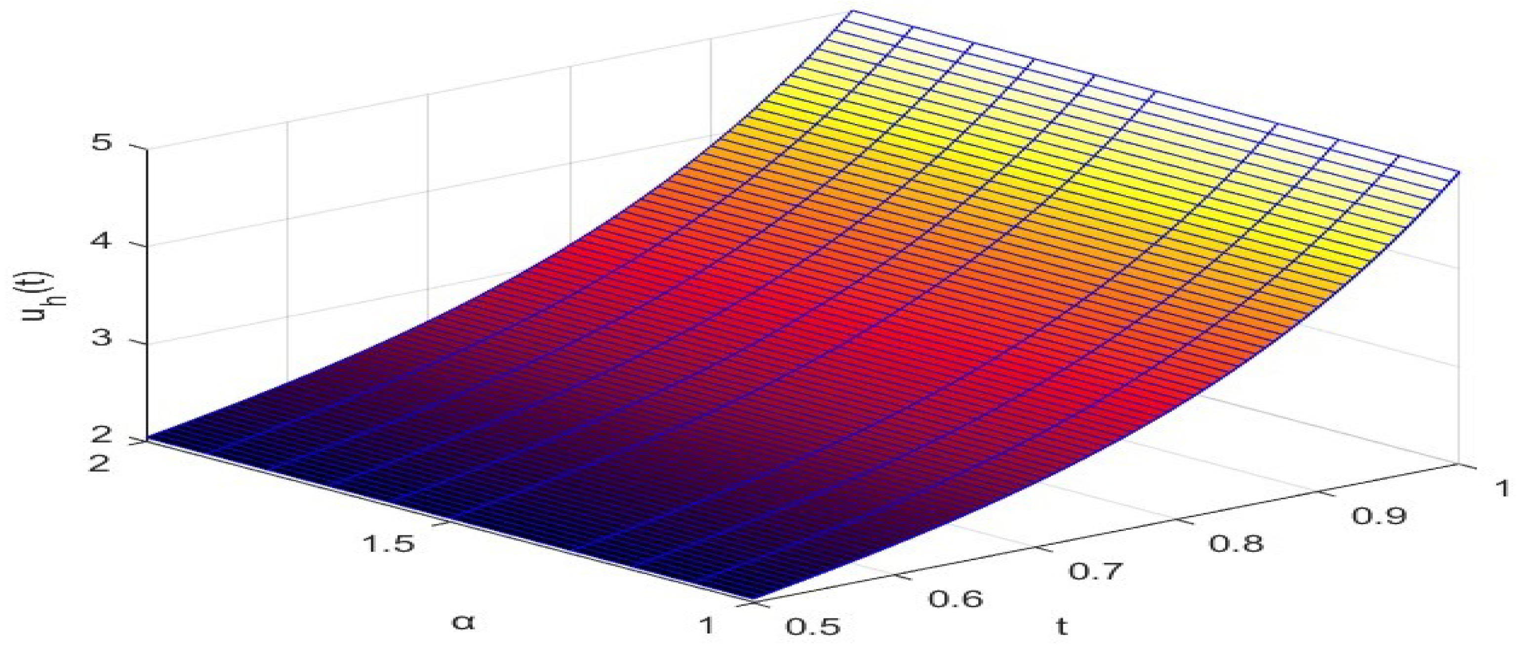
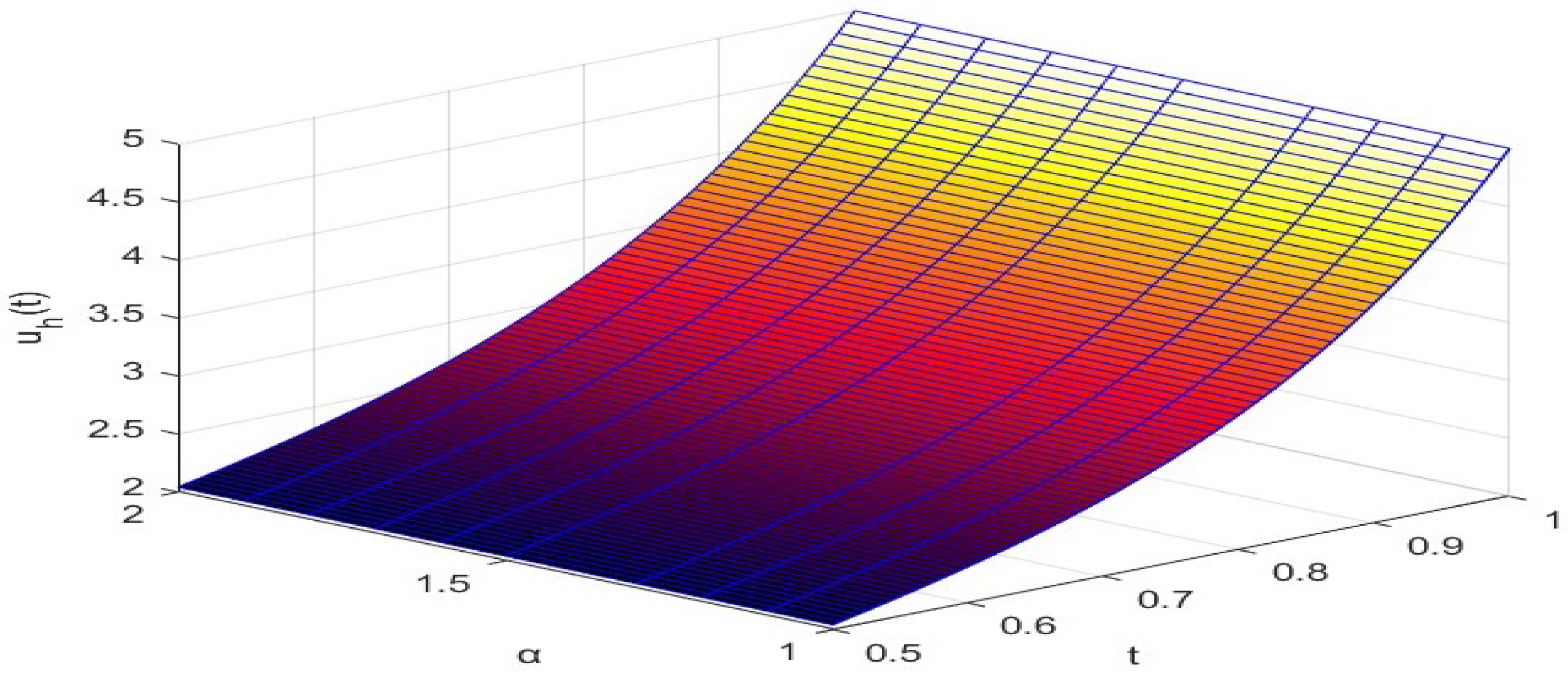
Figure 1 shows the approximate solution $u_h$, and Figure 2 illustrates the absolute error function $A{E}_h$ for Example 1 when $N=40,m=3$ with respect to $\varpi$ using the M-CP as collocation parameters.

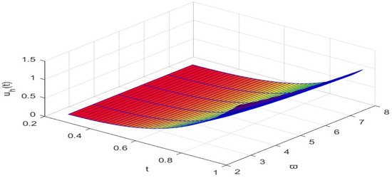
Figure 1. The graph of the approximate solution $u_h$ for Example 1 when $N=40,m=3$ with respect to $\varpi$ using the M-CP.

Figure 2. The graph of the $A{E}_h$ for Example 1 when $N=40,m=3$ with respect to $\varpi$ using the M-CP.

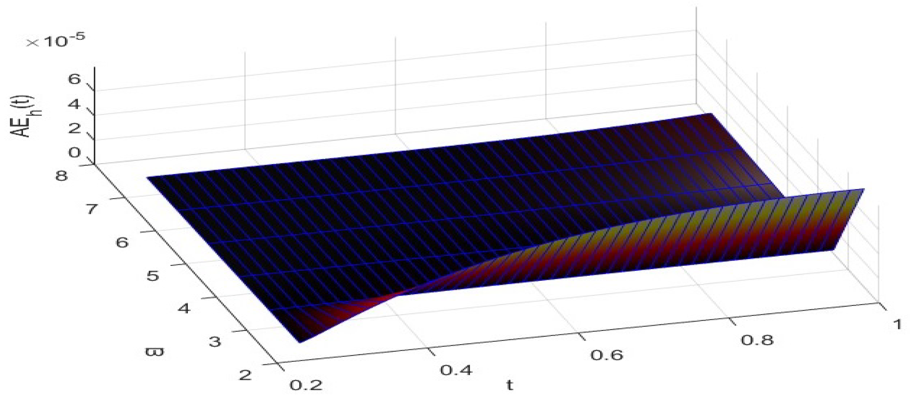
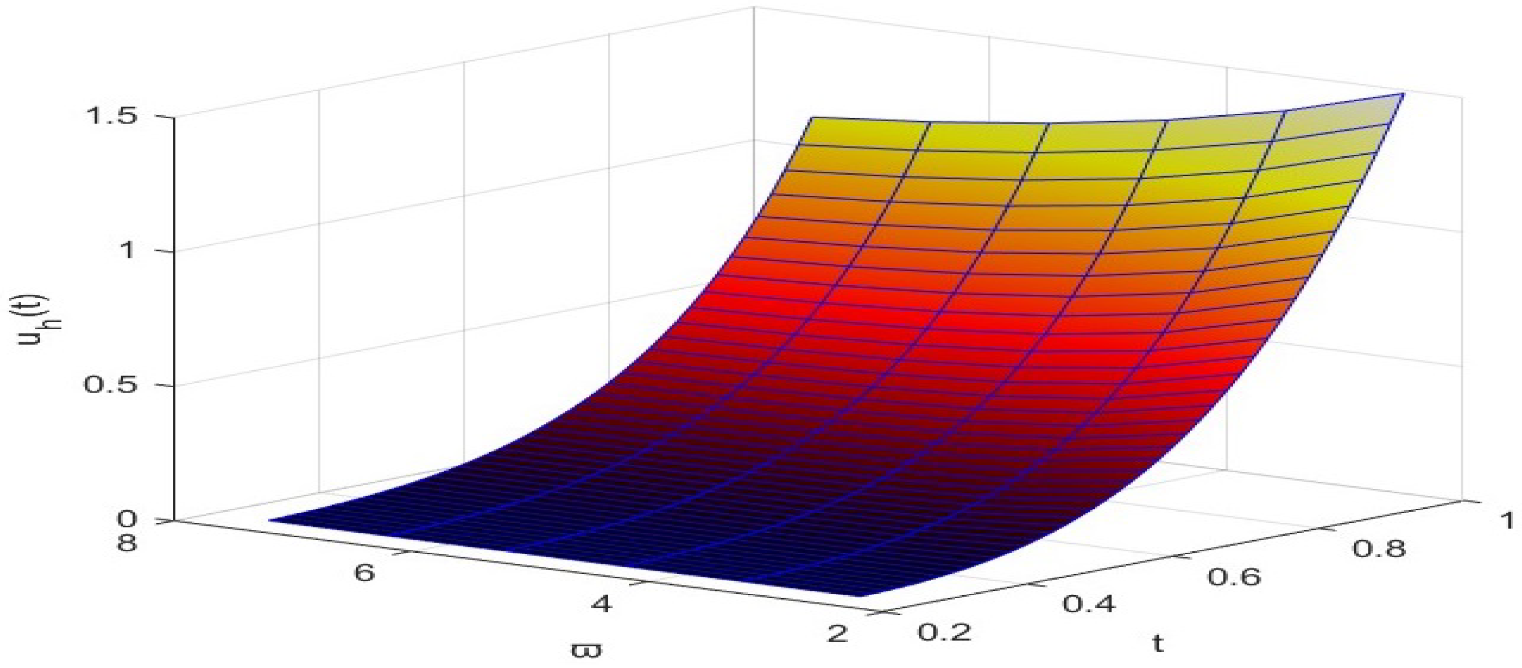
Figure 3 gives the graph of the approximate solution $u_h$ depending on $\varpi$, while Figure 4 presents the graph of $A{E}_h$ with respect to $\varpi$, both by using the G-LP and $N=40,m=3$ for Example 1. We see from Figure 2 and Figure 4 that the $A{E}_h$ is higher when the regularity parameter is taken as 5/2 and 7/2.

Figure 3. The graph of approximate solution $u_h$ for Example 1 when $N=40,m=3$ with respect to $\varpi$ using the G-LP.

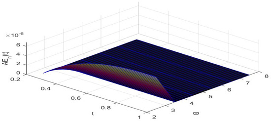
Figure 4. The graph of the $A{E}_h$ for Example 1 when $N=40,m=3$ depending on $\varpi$ using the G-LP.

Example 2.

This is an example where the fractional order α is not fixed, i.e., $1<\alpha <2$, and the exact solution y is smooth:

$$t^2{D}^{2}y\left(t\right)+t^{\alpha }{}_{\frac{1}{2}}{}^{C}D_t^{\alpha }y\left(t\right)+y\left(t\right)=f\left(t\right),t\in \left(\frac{1}{2},1\right),$$

is subject to

$$y\left({\displaystyle \frac{1}{2}}\right)={\displaystyle \frac{1}{2^{\frac{13}{2}}}}+{\displaystyle \frac{65}{32}},y^{\prime }\left({\displaystyle \frac{1}{2}}\right)={\displaystyle \frac{13}{2(2^{\frac{11}{2}})}}+{\displaystyle \frac{37}{16}},$$

where the exact solution and the non-homogeneous term are

$$\begin{array}{ccc}\hfill y\left(t\right)& =& t^{\frac{13}{2}}+t^5+2t+1,\hfill \\ \hfill f\left(t\right)& =& \frac{1}{4}{t}^5\left(80+143t^{\frac{3}{2}}\right)+t^{\frac{13}{2}}+t^5+2t+1\hfill \\ & & +\frac{1}{128\Gamma (2-\alpha )}{t}^{\alpha }(\frac{1}{(-5+\alpha )(-4+\alpha )(-3+\alpha )(-2+\alpha )}\hfill \\ & & \times 5\left(2^{4+\alpha }\right){(2t-1)}^{2-\alpha }(24-26\alpha -{\alpha }^3-6\alpha t(5+4t)+{\alpha }^2(9+6t)+12t(3+4t(1+t)))\hfill \\ & & +\left.13t^{-\alpha }\left({\displaystyle \frac{10395\sqrt{\pi }{t}^{\frac{13}{2}}\Gamma (2-\alpha )}{\Gamma (\frac{15}{2}-\alpha )}}-\sqrt{2}t{}_{2}F_1\left[{\displaystyle \frac{11}{2}},-1+\alpha ,{\displaystyle \frac{13}{2}},{\displaystyle \frac{1}{2t}}\right]\right)\right).\hfill \end{array}$$

In this example, the proposed Algorithm 1 is also applied for $m=3$. Table 3 gives the $MA{E}_h$, $E_2^h$, and the ratios $R_{h,\frac{h}{2}}^{\ast }$, $R_{h,\frac{h}{2}}$ and the determinant of matrix $A^{\left(0\right)}$ for various values of N and $\alpha$ when M-CP is used. A close look at the ratios indicates that the numerical method gives third-order convergence $\mathcal{O}\left(h^3\right)$, remarking that $R_{h,\frac{h}{2}}^{\ast }\approx 2^3$ and $R_{h,\frac{h}{2}}\approx {\left(2^3\right)}^2$. The analogous quantities are presented in Table 4 for G-LP.

Table 3. The error norms, convergence orders, and $det{A}^{\left(0\right)}$ for Example 2 obtained by using the M-CP.

$\mathit{\alpha }$	N	${\mathit{MAE}}_{\mathit{h}}$	${\mathit{R}}_{\mathit{h},\frac{\mathit{h}}{2}}^{\ast }$	${\mathit{E}}_2^{\mathit{h}}$	${\mathit{R}}_{\mathit{h},\frac{\mathit{h}}{2}}$	${\mathit{detA}}^{\left(0\right)}$
$1.5$	10	$1.2612\times {10}^{-4}$		$1.5442\times {10}^{-9}$		$0.118010$
	20	$1.5152\times {10}^{-5}$	$8.3237$	$2.1882\times {10}^{-11}$	$70.5694$	$0.082311$
	40	$1.8573\times {10}^{-6}$	$8.1581$	$3.2595\times {10}^{-13}$	$67.1330$	$0.066086$
	80	$2.3000\times {10}^{-7}$	$8.0752$	$4.9500\times {10}^{-15}$	$65.8485$	$0.057684$
$1.3$	10	$1.3570\times {10}^{-4}$		$1.7942\times {10}^{-9}$		$0.089907$
	20	$1.6443\times {10}^{-5}$	$8.2528$	$2.5876\times {10}^{-11}$	$69.3384$	$0.065772$
	40	$2.0252\times {10}^{-6}$	$8.1192$	$3.8923\times {10}^{-13}$	$66.4800$	$0.055313$
	80	$2.5143\times {10}^{-7}$	$8.0547$	$5.9420\times {10}^{-15}$	$65.5049$	$0.050279$
$1.2$	10	$1.4165\times {10}^{-4}$		$1.9556\times {10}^{-9}$		$0.082713$
	20	$1.7164\times {10}^{-5}$	$8.2527$	$2.8206\times {10}^{-11}$	$69.3328$	$0.061921$
	40	$2.1129\times {10}^{-6}$	$8.1234$	$4.2386\times {10}^{-13}$	$66.5456$	$0.053035$
	80	$2.6218\times {10}^{-7}$	$8.0590$	$6.4633\times {10}^{-15}$	$65.5795$	$0.048861$
$1.1$	10	$1.4759\times {10}^{-4}$		$2.1221\times {10}^{-9}$		$0.078016$
	20	$1.7860\times {10}^{-5}$	$8.2637$	$3.0525\times {10}^{-11}$	$69.5201$	$0.059551$
	40	$2.1963\times {10}^{-6}$	$8.1319$	$4.5767\times {10}^{-13}$	$66.6965$	$0.051716$
	80	$2.7231\times {10}^{-7}$	$8.0654$	$6.9675\times {10}^{-15}$	$65.6864$	$0.048091$
$1.001$	10	$1.5317\times {10}^{-4}$		$2.2826\times {10}^{-9}$		$0.074978$
	20	$1.8503\times {10}^{-5}$	$8.2781$	$3.2713\times {10}^{-11}$	$69.7765$	$0.058109$
	40	$2.2727\times {10}^{-6}$	$8.1414$	$4.8929\times {10}^{-13}$	$66.8581$	$0.050963$
	80	$2.8158\times {10}^{-7}$	$8.0712$	$7.4374\times {10}^{-15}$	$65.7878$	$0.047679$

Table 4. The error norms, convergence orders, and $det{A}^{\left(0\right)}$ for Example 2 obtained using G-LP.

$\mathit{\alpha }$	N	${\mathit{MAE}}_{\mathit{h}}$	${\mathit{R}}_{\mathit{h},\frac{\mathit{h}}{2}}^{\ast }$	${\mathit{E}}_2^{\mathit{h}}$	${\mathit{R}}_{\mathit{h},\frac{\mathit{h}}{2}}$	$\mathit{det}\left({\mathit{A}}^0\right)$
$1.5$	10	$1.5523\times {10}^{-7}$		$2.8048\times {10}^{-15}$		$0.520922$
	20	$1.3358\times {10}^{-8}$	$11.6208$	$1.8408\times {10}^{-17}$	$152.3685$	$0.405034$
	40	$1.1620\times {10}^{-9}$	$11.4957$	$1.3516\times {10}^{-19}$	$136.1941$	$0.347087$
	80	$1.0184\times {10}^{-10}$	$11.4101$	$1.0229\times {10}^{-21}$	$132.1341$	$0.315164$
$1.3$	10	$4.5573\times {10}^{-8}$		$4.0353\times {10}^{-16}$		$0.417067$
	20	$3.3904\times {10}^{-9}$	$13.4418$	$1.3828\times {10}^{-18}$	$291.8209$	$0.338744$
	40	$2.5551\times {10}^{-10}$	$13.2691$	$6.8916\times {10}^{-21}$	$200.6501$	$0.301922$
	80	$1.9437\times {10}^{-11}$	$13.1455$	$3.8457\times {10}^{-23}$	$179.2027$	$0.283354$
$1.2$	10	$2.0151\times {10}^{-8}$		$2.0179\times {10}^{-16}$		$0.392175$
	20	$1.3926\times {10}^{-9}$	$14.4701$	$3.6027\times {10}^{-19}$	$560.1077$	$0.324243$
	40	$9.7632\times {10}^{-11}$	$14.2638$	$1.1446\times {10}^{-21}$	$314.7562$	$0.292946$
	80	$6.9171\times {10}^{-12}$	$14.1146$	$5.0524\times {10}^{-24}$	$226.5458$	$0.277638$
$1.1$	10	$6.5025\times {10}^{-9}$		$1.5170\times {10}^{-16}$		$0.376448$
	20	$4.1659\times {10}^{-10}$	$15.6089$	$1.6210\times {10}^{-19}$	$935.8421$	$0.315603$
	40	$2.7153\times {10}^{-11}$	$15.3423$	$2.1777\times {10}^{-22}$	$744.3633$	$0.287919$
	80	$1.7906\times {10}^{-12}$	$15.1642$	$4.6867\times {10}^{-25}$	$464.6553$	$0.274636$
$1.001$	10	$7.7479\times {10}^{-11}$		$1.4279\times {10}^{-16}$		$0.366557$
	20	$3.0056\times {10}^{-12}$	$25.7782$	$1.3932\times {10}^{-19}$	$1024.9067$	$0.310488$
	40	$1.5632\times {10}^{-13}$	$19.2272$	$1.3602\times {10}^{-22}$	$1024.2611$	$0.285126$
	80	$8.8818\times {10}^{-15}$	$17.6000$	$1.3247\times {10}^{-25}$	$1026.7985$	$0.273074$

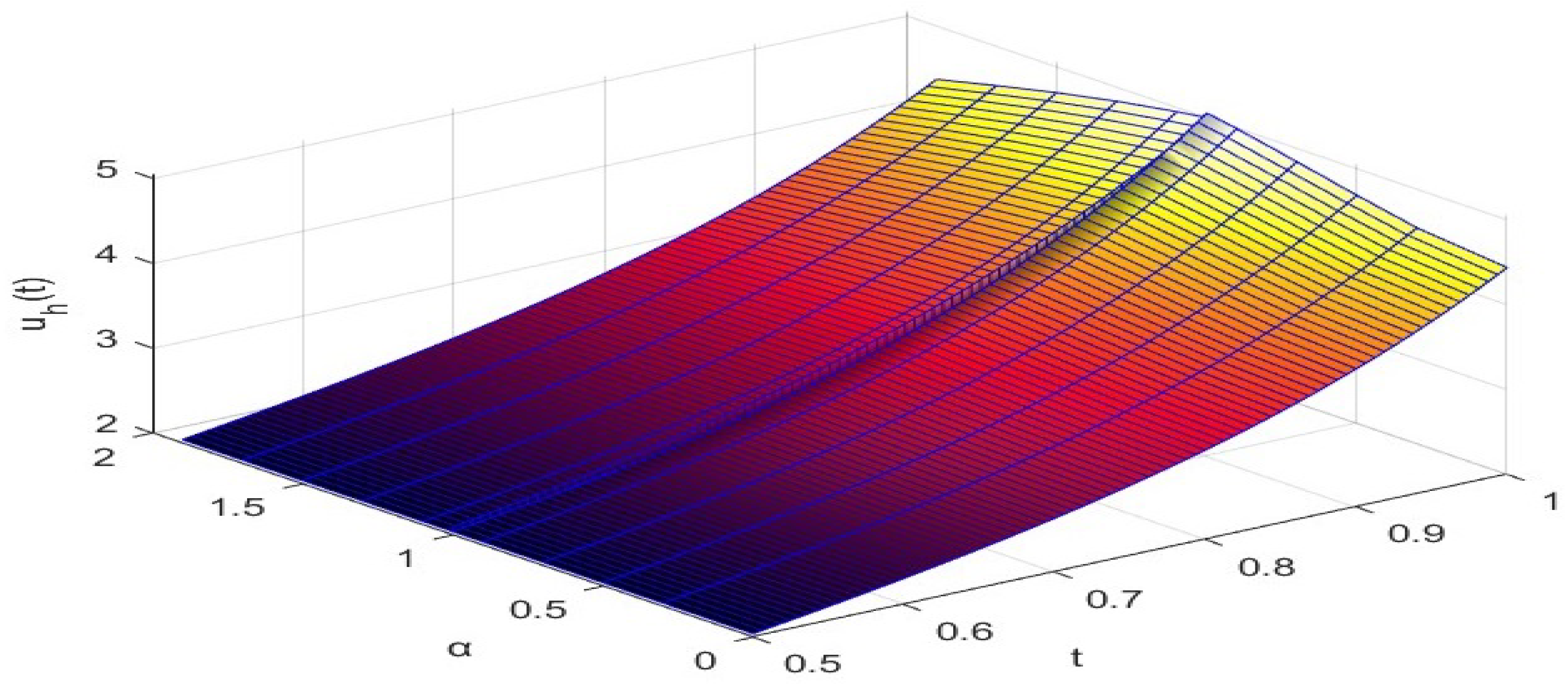
Figure 5 shows the graph of the approximate solution $u_h$, and Figure 6 demonstrates the absolute error $A{E}_h$ both with respect to $\alpha$ for Example 2 when $N=80,m=3$ using the M-CP. Further, the functions $u_h$ and $A{E}_h$ with respect to $\alpha$ for the same parameters are shown in Figure 7 and Figure 8, respectively, using the G-LP. We view from Figure 6 and Figure 8 that the absolute error is higher near the corner $(t,\alpha )=(1,2)$. These figures justify a good approximation of the exact solution.

Figure 5. The graph of the approximate solution $u_h$ for $N=80,m=3$ with respect to $\alpha$ using the M-CP for Example 2.

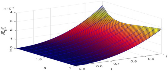
Figure 6. The graph of the $A{E}_h$ for $N=80,m=3$ with respect to $\alpha$ using the M-CP for Example 2.

Figure 7. The graph of the approximate solution $u_h$ for $N=80,m=3$ with respect to $\alpha$ using the G-LP for Example 2.

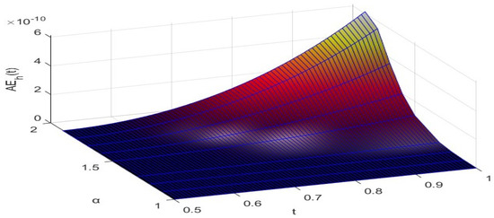
Figure 8. The graph of the $A{E}_h$ with respect to $\alpha$ when $N=80,m=3$ using the G-LP for Example 2.

Example 3.

This is an example in which the exact solution is unknown. Consider the following problem:

$$\begin{array}{c}\hfill t^2{D}^{2}y\left(t\right)+t^{\alpha }{}_{\frac{1}{2}}{}^{C}D_t^{\alpha }y\left(t\right)+y\left(t\right)=f\left(t\right),t\in \left(\frac{1}{2},1\right),\\ \hfill y\left(\frac{1}{2}\right)=\frac{1}{2^{\frac{13}{2}}}+\frac{65}{32}{y}^{\prime }\left(\frac{1}{2}\right)=\frac{13}{2(2^{\frac{11}{2}})}+\frac{37}{16},\end{array}$$

where $0<\alpha <2$, and the exact solution y is unknown, and

$$f\left(t\right)=\{\begin{array}{cc}26t^5-\frac{173}{4}{t}^{\frac{13}{2}}+4t+1,\hfill & \mathrm{if}0<\alpha ⩽1\\ \hfill 26t^5-\frac{173}{4}{t}^{\frac{13}{2}}+t\left(4-y^{\prime }\left(\frac{1}{2}\right)\right)+1,& \mathrm{if}1<\alpha <2.\end{array}$$

The problem in Example 3 reduces to the classical Cauchy–Euler problem for $\alpha =1$ with the exact solution $y\left(t\right)=t^{13/2}+t^5+2t+1$. Table 5 shows the approximate solution $u_h$ of the problem in Example 3 at some mesh points obtained by using the G-LP when $N=80,m=4$, for $0<\alpha <1$ and $1<\alpha <2$. Table 5 also presents the exact solution when $\alpha =1$. Further, Table 6 gives the approximate solution $u_h$, for $h={\displaystyle \frac{1}{40}},{\displaystyle \frac{1}{80}},{\displaystyle \frac{1}{160}}$ and the convergence order when $\alpha =1.0001$ and $\alpha =0.9999$ for Example 3 for $m=4$ by using G-LP for collocation. In Table 6, na means the order is not available at that point since the error is 0. Additionally, Table 7 presents the total computational time required for applying the algorithm for Example 3 when G-LP and M-CP points are used as collocation parameters. It can be concluded from this table that the total computational time varies linearly with respect to N. Finally, Figure 9 illustrates the graph of the approximate solution $u_h$ for $N=80,m=4$, $0<\alpha <2$ for Example 3 using the G-LP for collocation.

Table 5. The approximate solution $u_h$ obtained by using the G-LP when $0<\alpha <1$, $1<\alpha <2$ and $N=80,m=4$, and the exact solution when $\alpha =1$ for Example 3.

t	$\mathit{\alpha }=0.0000001$	$\mathit{\alpha }=0.3$	$\mathit{\alpha }=0.5$	$\mathit{\alpha }=0.7$	$\mathit{\alpha }=0.9$	$\mathit{\alpha }=0.9999$	$\mathit{\alpha }=1$
0.50	2.0422985435	2.0422985435	2.0422985435	2.0422985435	2.0422985435	2.0422985435	2.0422985435
0.55	2.1767805121	2.1764037955	2.1758232163	2.1746903204	2.1725380227	2.1708588887	2.1708569500
0.60	2.3369024513	2.3347716925	2.3319658673	2.3271986993	2.3193731879	2.3139056592	2.3138995822
0.65	2.5274156028	2.5216636520	2.5147425376	2.5038899232	2.4875408103	2.4768453377	2.4768337160
0.70	2.7549968510	2.7434643682	2.7304274618	2.7110949449	2.6836631424	2.6665205545	2.6665022155
0.75	3.0284929630	3.0087827046	2.9875216050	2.9572869381	2.9162563165	2.8914648279	2.8914386034
0.80	3.3592046620	3.3286793244	3.2969387426	3.2532481862	3.1959458560	3.1621841421	3.1621487216
0.85	3.7612101952	3.7169586037	3.6722763258	3.6123322973	3.5357501179	3.4914661707	3.4914199851
0.90	4.2517280048	4.1905099616	4.1301429778	4.0507848212	3.9514084005	3.8947180844	3.8946592006
0.95	4.8515182766	4.7696929559	4.6905325451	4.5881098490	4.4617466989	4.3903338681	4.3902598857
1.00	5.5853233461	5.4787636267	5.3772403414	5.2474775023	5.0890786630	5.0000920558	5.0000000000
t	$\mathit{\alpha }=\mathbf{1.9}$	$\mathit{\alpha }=\mathbf{1.7}$	$\mathit{\alpha }=\mathbf{1.5}$	$\mathit{\alpha }=\mathbf{1.3}$	$\mathit{\alpha }=\mathbf{1.1}$	$\mathit{\alpha }=\mathbf{1.01}$	$\mathit{\alpha }=\mathbf{1.00001}$
0.50	2.0422985435	2.0422985435	2.0422985435	2.0422985435	2.0422985435	2.0422985435	2.0422985435
0.55	2.1685531044	2.1694376642	2.1701085260	2.1705384260	2.1707822586	2.1708505494	2.1708569437
0.60	2.3034979414	2.3069732352	2.3098697446	2.3120010835	2.3134119334	2.3138562759	2.3138995394
0.65	2.4506782624	2.4587657163	2.4658149461	2.4713707428	2.4753607944	2.4767003017	2.4768335840
0.70	2.6146277713	2.6298871983	2.6435414918	2.6547572542	2.6632359905	2.6662024934	2.6665019185
0.75	2.8009911854	2.8266990317	2.8500965497	2.8698446529	2.8853034382	2.8908703942	2.8914380399
0.80	3.0166988503	3.0570373680	3.0941795395	3.1261217059	3.1517532229	3.1611793495	3.1621477597
0.85	3.2701646359	3.3304340391	3.3863863632	3.4351515048	3.4749961111	3.4898805355	3.4914184567
0.90	3.5715038824	3.6583631732	3.7394835794	3.8108721430	3.8699896105	3.8923376437	3.8946568947
0.95	3.9327709570	4.0545114009	4.1687095689	4.2699264243	4.3545935706	4.3868930719	4.3902565406
1.00	4.3682166429	4.5350713106	4.6921020473	4.8320202532	4.9499557991	4.9952644911	4.9999952937

Table 6. The approximate solution $u_h$, for $h=\frac{1}{40},\frac{1}{80},\frac{1}{160}$ obtained by using the G-LP when $\alpha =1.0001$, $\alpha =0.9999$ and $N=80,m=4$, and the exact solution when $\alpha =1$ for Example 3.

			$\mathit{\alpha }=1.0001$
t	${\mathit{u}}_{\frac{\mathbf{1}}{\mathbf{40}}}$	${\mathit{u}}_{\frac{\mathbf{1}}{\mathbf{80}}}$	${\mathit{u}}_{\frac{\mathbf{1}}{\mathbf{160}}}$	$\left|{\mathit{u}}_{\frac{\mathbf{1}}{\mathbf{80}}}-{\mathit{u}}_{\frac{\mathbf{1}}{\mathbf{40}}}\right|$	$\left|{\mathit{u}}_{\frac{\mathbf{1}}{\mathbf{160}}}-{\mathit{u}}_{\frac{\mathbf{1}}{\mathbf{80}}}\right|$	$\left|\frac{{\mathit{u}}_{\frac{\mathbf{1}}{\mathbf{80}}}-{\mathit{u}}_{\frac{\mathbf{1}}{\mathbf{40}}}}{{\mathit{u}}_{\frac{\mathbf{1}}{\mathbf{160}}}-{\mathit{u}}_{\frac{\mathbf{1}}{\mathbf{80}}}}\right|$	${\mathit{log}}_{\mathbf{2}}\left|\frac{{\mathit{u}}_{\frac{\mathbf{1}}{\mathbf{80}}}-{\mathit{u}}_{\frac{\mathbf{1}}{\mathbf{40}}}}{{\mathit{u}}_{\frac{\mathbf{1}}{\mathbf{160}}}-{\mathit{u}}_{\frac{\mathbf{1}}{\mathbf{80}}}}\right|$
$0.5$	$2.042298543456040$	$2.042298543456040$	$2.042298543456040$	0	0	na	na
$0.6$	$2.313899148354915$	$2.313899154236738$	$2.313899154719453$	$5.88182\times {10}^{-9}$	$4.82715\times {10}^{-10}$	$12.18488$	$3.60702$
$0.7$	$2.666499225421245$	$2.666499245233377$	$2.666499246682199$	$1.98121\times {10}^{-8}$	$1.44882\times {10}^{-9}$	$13.67465$	$3.77343$
$0.8$	$3.162139059025395$	$3.162139100430150$	$3.162139103305870$	$4.14048\times {10}^{-8}$	$2.87572\times {10}^{-9}$	$14.39805$	$3.84780$
$0.9$	$3.894636067629396$	$3.894636138137670$	$3.894636142895072$	$7.05083\times {10}^{-8}$	$4.75740\times {10}^{-9}$	$14.82075$	$3.88955$
$1.0$	$4.999952824239302$	$4.999952931336956$	$4.999952938431949$	$1.07098\times {10}^{-7}$	$7.09499\times {10}^{-9}$	$15.09482$	$3.91598$
			$\mathit{\alpha }=\mathbf{0}.\mathbf{9999}$
t	${\mathit{u}}_{\frac{\mathbf{1}}{\mathbf{40}}}$	${\mathit{u}}_{\frac{\mathbf{1}}{\mathbf{80}}}$	${\mathit{u}}_{\frac{\mathbf{1}}{\mathbf{160}}}$	$\left|{\mathit{u}}_{\frac{\mathbf{1}}{\mathbf{80}}}-{\mathit{u}}_{\frac{\mathbf{1}}{\mathbf{40}}}\right|$	$\left|{\mathit{u}}_{\frac{\mathbf{1}}{\mathbf{160}}}-{\mathit{u}}_{\frac{\mathbf{1}}{\mathbf{80}}}\right|$	$\left|\frac{{\mathit{u}}_{\frac{\mathbf{1}}{\mathbf{80}}}-{\mathit{u}}_{\frac{\mathbf{1}}{\mathbf{40}}}}{{\mathit{u}}_{\frac{\mathbf{1}}{\mathbf{160}}}-{\mathit{u}}_{\frac{\mathbf{1}}{\mathbf{80}}}}\right|$	${\mathit{log}}_{\mathbf{2}}\left|\frac{{\mathit{u}}_{\frac{\mathbf{1}}{\mathbf{80}}}-{\mathit{u}}_{\frac{\mathbf{1}}{\mathbf{40}}}}{{\mathit{u}}_{\frac{\mathbf{1}}{\mathbf{160}}}-{\mathit{u}}_{\frac{\mathbf{1}}{\mathbf{80}}}}\right|$
$0.5$	$2.042298543456040$	$2.042298543456040$	$2.042298543456040$	0	0	na	na
$0.6$	$2.336382834484979$	$2.336382890186138$	$2.336382904938831$	$5.57012\times {10}^{-8}$	$1.47527\times {10}^{-8}$	$3.77566$	$1.90917$
$0.7$	$2.751974647483427$	$2.751974754449280$	$2.751974782928411$	$1.06966\times {10}^{-7}$	$2.84791\times {10}^{-8}$	$3.75594$	$1.90644$
$0.8$	$3.350897309586328$	$3.350897463143591$	$3.350897504104982$	$1.53557\times {10}^{-7}$	$4.09614\times {10}^{-8}$	$3.74883$	$1.90494$
$0.9$	$4.234669738339650$	$4.234669933390302$	$4.234669985474072$	$1.95051\times {10}^{-7}$	$5.20838\times {10}^{-8}$	$3.74494$	$1.90395$
$1.0$	$5.555168946791253$	$5.555169178255524$	$5.555169240105265$	$2.31464\times {10}^{-7}$	$6.18497\times {10}^{-8}$	$3.74236$	$1.90917$

Table 7. The total computational time (CPU(s)) with respect to N obtained when G-LP and M-CP are used.

N	10	20	40	80	160	320
G-LP	1.19	2.12	3.17	6.25	13.33	27.63
M-CP	1.06	2.03	3.94	7.96	13.50	28.21

Figure 9. The graph of the approximate solution $u_h\left(t\right)$ for $N=80,m=4$ and $0<\alpha <2$ for Example 3 using the G-LP for collocation.

6. Conclusions

A fractional Cauchy–Euler problem in the Caputo sense is studied. The existence and uniqueness of the solution are investigated using the contracting mapping principle. Further, a collocation method and an algorithm is given for the numerical solution. Additionally, convergence analyses are provided, and the developed method is applied on some constructed fractional Cauchy–Euler (FrC-E) problems. The simulations justify the theoretical results.

In future research, the authors may consider discussing the potential extension of their method, specifically the application of the proposed numerical approach to higher-dimensional Caputo fractional Cauchy–Euler problems. This could be advantageous for addressing more complex systems. The authors can also conduct an error analysis to pinpoint possible sources of numerical inaccuracies and enhance the algorithm for improved precision and stability.

Moreover, they will consider the effectiveness of their method using different types of fractional derivatives operators, such as the Riemanns–Liouville or Grunwald–Letnikov derivatives.

References

- Touma, R.; Zeidan, D. An unstaggered central finite volume method for the numerical approximation of mixture flows. In Proceedings of the International Conference of Numerical Analysis and Applied Mathematics (ICNAAM), Rhodes, Greece, 23–28 September 2019. [Google Scholar]
- Bahia, G.; Ouannas, A.; Batiha, I.M.; Odibat, Z. The optimal homotopy analysis method applied on nonlinear time-fractional hyperbolic partial differential equations. Numer. Methods Partial. Differ. Equ. 2021, 37, 2008–2022. [Google Scholar] [CrossRef]
- Torvik, P.J.; Bagley, R.L. On the appearance of the fractional derivative in the behavior of real materials. J. Appl. Mech. 1984, 51, 294–298. [Google Scholar] [CrossRef]
- Wei, H.M.; Zhong, X.C.; Huang, Q.A. Uniqueness and approximation of solution for fractional Bagley–Torvik equations with variable coefficients. Int. J. Comput. Math. 2017, 94, 1542–1561. [Google Scholar] [CrossRef]
- Zhong, X.; Liu, X.; Liao, S. On a generalized Bagley–Torvik equation with a fractional integral boundary condition. Int. J. Appl. Comput. 2017, 3, 727–746. [Google Scholar] [CrossRef]
- Irmak, H. Some computational results for functions belonging to a family consisting of Cauchy-Euler type differential equation. Fract. Differ. Calc. 2012, 2, 109–117. [Google Scholar] [CrossRef]
- Mazur, D.; Marek, K. Analysis and Simulation of Electrical and Computer Systems; Springer: Cham, Switzerland, 2018. [Google Scholar]
- Kilbas, A.A.; Rivero, M.; Trujillo, J.J. Euler-Type Fractional Differential Equations. In Proceedings of the 5th International ISAAC Congress, Catania, Italy, 25–30 July 2005. [Google Scholar]
- Debnath, L.; Bhatta, D. Integral Transforms and Their Applications; Chapman and Hall/CRC: New York, NY, USA, 2016. [Google Scholar]
- Zhukovskaya, N.V.; Kilbas, A.A. Solving homogeneous fractional differential equations of Euler type. Differ. Equ. 2011, 47, 1714–1725. [Google Scholar] [CrossRef]
- Kilbas, A.A.; Zhukovskaya, N.V. Euler-type non-homogeneous differential equations with three Liouville fractional derivatives. Fract. Calc. Appl. Anal. 2009, 12, 206–234. [Google Scholar]
- Erdélyi, A.; Magnus, W.; Oberhettinger, F.; Tricomi, F.G. Table Errata: Higher Transcendental Functions, Volume I, II; McGraw-Hill: New York, NY, USA, 1953. [Google Scholar]
- Zhukovskaya, N.V. Solutions of Euler-type homogeneous differential equations with finite number of fractional derivatives. Integral Transform. Spec. Funct. 2012, 23, 161–175. [Google Scholar] [CrossRef]
- Simmons, G.F. Differential Equations with Applications and Historical Notes; CRC Press: New York, NY, USA, 2016. [Google Scholar]
- Granas, A.; Guenther, R.B.; Lee, J.W. Nonlinear boundary value problems for ordinary differential equations. Diss. Math. (Rozpr. Mat.) 1985, 244, 128. [Google Scholar]
- O’Regan, D. Existence of positive solutions to some singular and nonsingular second order boundary value problems. J. Differ. Equ. 1990, 84, 228–251. [Google Scholar] [CrossRef]
- Young, N.F.; Tisdell, C.C. The existence of solutions to second-order singular boundary value problems. Nonlinear Anal. 2012, 75, 4798–4806. [Google Scholar] [CrossRef]
- Tisdell, C.C. Basic existence and a priori bound results for solutions to systems of boundary value problems for fractional differential equations. Electron. J. Differ. Equ. 2016, 2016, 1–9. [Google Scholar]
- Young, N.F. Existence results, inequalities and a priori bounds to fractional boundary value problems. Fract. Differ. Calc. 2021, 11, 175–191. [Google Scholar]
- Turqa, S.M.; Nuruddeen, R.I.; Nawaz, R. Recent advances in employing the Laplace homotopy analysis method to nonlinear fractional models for evolution equations and heat-typed problems. Int. J. Thermofluids 2024, 22, 100681. [Google Scholar] [CrossRef]
- Brunner, H. Collocation Methods for Volterra Integral and Related Functional Differential Equations; Cambridge University Press: London, UK, 2004; pp. 1–17. [Google Scholar]
- Al-Mdallal, Q.M.; Syam, M.I.; Anwar, M.N. A collocation-shooting method for solving fractional boundary value problems. Appl. Math. Comput. 2010, 15, 3814–3822. [Google Scholar] [CrossRef]
- Conte, D.; D’Ambrosio, R.; D’Arienzo, M.P.; Paternoster, B. Semi-implicit multivalue almost collocation methods. In Proceedings of the International Conference of Numerical Analysis and Applied Mathematics (ICNAAM), Rhodes, Greece, 17–23 September 2020. [Google Scholar]
- Zhang, X.; Du, H. An improved collocation method for solving a fractional integro-differential equation. Comput. Appl. Math. 2021, 40, 1–14. [Google Scholar] [CrossRef]
- Baleanu, D.; Shiri, B. Collocation methods for fractional differential equations involving non-singular kernel. Chaos Solitons Fractals 2018, 116, 136–145. [Google Scholar] [CrossRef]
- Eslahchi, M.; Dehghan, M.; Parvizi, M. Application of the collocation method for solving nonlinear fractional integro-differential equations. J. Comput. Appl. Math. 2014, 257, 105–128. [Google Scholar] [CrossRef]
- Rahimkhani, P.; Ordokhani, Y.; Lima, P.M. An improved composite collocation method for distributed-order fractional differential equations based on fractional Chelyshkov wavelets. Appl. Numer. Math. 2019, 145, 1–27. [Google Scholar] [CrossRef]
- Al-Mdallal, Q.M.; Omer, A.S. Fractional-order Legendre-collocation method for solving fractional initial value problems. Appl. Math. Comput. 2018, 321, 74–84. [Google Scholar] [CrossRef]
- Mirzaee, F.; Samadyar, N. On the numerical solution of fractional stochastic integro-differential equations via meshless discrete collocation method based on radial basis functions. Eng. Anal. Bound. Elem. 2019, 100, 246–255. [Google Scholar] [CrossRef]
- Mahmudov, I.N.; Buranay, S.C.; Chin, M.J. On a collocation method for the fractional Cauchy-Euler problem. In Proceedings of the International Conference of Numerical Analysis and Applied Mathematics 2023 (ICNAAM 2023), Crete, Greece, 11–16 September 2023. [Google Scholar]
- Rawashdeh, E.A. Numerical solution of semidifferential equations by collocation method. Appl. Math. Comput. 2006, 174, 869–876. [Google Scholar] [CrossRef]
- Buranay, S.C.; Chin, M.J.; Mahmudov, N.I. A collocation-shooting method for solving fractional boundary value problems for generalized Bagley Torvik equation. In Proceedings of the International Conference on Analysis and Applied Mathematics, Antalya, Turkey, 31 October–6 November 2022. [Google Scholar]
- Kilbas, A.A.; Srivastava, H.M.; Trujillo, J.J. Theory and Applications of Fractional Differential Equations; Elsevier: Amsterdam, The Netherlands, 2006; pp. 1–523. [Google Scholar]
- Abramowitz, M.; Stegun, I.A. Handbook of Mathematical Functions with Formulas, Graphs, and Mathematical Tables; US Government Printing Office: Washington, DC, USA, 1968.
Disclaimer/Publisher’s Note: The statements, opinions and data contained in all publications are solely those of the individual author(s) and contributor(s) and not of MDPI and/or the editor(s). MDPI and/or the editor(s) disclaim responsibility for any injury to people or property resulting from any ideas, methods, instructions or products referred to in the content. |
© 2024 by the authors. Licensee MDPI, Basel, Switzerland. This article is an open access article distributed under the terms and conditions of the Creative Commons Attribution (CC BY) license (https://creativecommons.org/licenses/by/4.0/).