Energy-Conserving Explicit Relaxed Runge–Kutta Methods for the Fractional Nonlinear Schrödinger Equation Based on Scalar Auxiliary Variable Approach

Abstract

In this paper, we present a novel explicit structure-preserving numerical method for solving nonlinear space-fractional Schrödinger equations based on the concept of the scalar auxiliary variable approach. Firstly, we convert the equations into an equivalent system through the introduction of a scalar variable. Subsequently, a semi-discrete energy-preserving scheme is developed by employing a fourth-order fractional difference operator to discretize the equivalent system in spatial direction, and obtain the fully discrete version by using an explicit relaxed Runge–Kutta method for temporal integration. The proposed method preserves the energy conservation property of the space-fractional nonlinear Schrödinger equation and achieves high accuracy. Numerical experiments are carried out to verify the structure-preserving qualities of the proposed method.

1. Introduction

Fractional differential equations have been effectively utilized in many fields, including chemistry, physics, biology, and hydrology [1]. The classical Schrödinger equation stands as a foundation of quantum mechanics. By extending quantum mechanics based on the path integral over Lévy-like quantum-mechanical paths, the fractional Schrödinger equations can be obtained. During the past decades, the space-fractional nonlinear Schrödinger (F-NLS) equation has attracted more and more scholars’ interest. Some mathematical properties of F-NLS equations, such as the well-posedness and energy preservation, as well as many physical properties and applications, have been given in the literature, see [2,3,4] for example.

However, due to the intricacy of nonlinear terms and the intangible functions included in analytical solutions, finding an exact solution is difficult. Thus, efficiently developing accurate, reliable, and easy-to-implement numerical methods for the F-NLS equation naturally becomes an urgent topic.

In this context, we consider the F-NLS equation as follows

$$\begin{array}{c}\hfill \mathrm{i}{\displaystyle \frac{\partial u\left(x,t\right)}{\partial t}}+{\displaystyle \frac{1}{2}}{\left(-△\right)}^{{\displaystyle \frac{\alpha }{2}}}u\left(x,t\right)+\rho {\left|u\left(x,t\right)\right|}^{2}u\left(x,t\right)=0,(x,t)\in R_d\times (0,T],\end{array}$$

subject to the initial conditions

$$\begin{array}{c}\hfill u\left(x,0\right)=\psi \left(x\right),x\in R_d,\end{array}$$

(1)

and the periodic boundary condition

$$\begin{array}{c}\hfill u\left(x+\delta e_j,t\right)=u\left(x,t\right),(x,t)\in R_d\times (0,T],\end{array}$$

where $\mathrm{i}=\sqrt{-1}$ is the imaginary unit, $u(x,t)$ is a complex-valued wave function on $t\in \left(0,T\right]$, and $x\in R_d$ for $d=\{1,2,3\}$. Equation (1) is written in multi-dimensions. The parameter $\rho$ describes the strength of short-range (or local) nonlinear interactions: when $\rho$ is positive, the interactions are repulsive or defocusing, whereas, if $\rho$ is negative, the interactions are attractive or focusing [5]. $e_j=(0,\cdots ,0,1,0,\cdots ,0)$, $j=1,2,\cdots ,n$ denotes an orthonormal basis of $R_d$, where $\delta >0$ signifies a periodic cycle. Generally, we can select a sufficiently large domain, D, so that the solution outside D becomes negligible because of the algebraic decay of $u(x,t)$ in space. This domain, D, can be modeled as a periodic region with Dirichlet boundary conditions. Therefore, we can consider an approximation to the original problem’s solution as the solution of the F-NLS equation with periodic boundaries when T is fixed [6]. In this sense, we will, without loss of generality, focus solely on the problem within the periodic region $D=(a,b)\times \cdots \times (a,b)\subset {\mathbb{R}}^d$. The fractional Laplacian ${(-\mathsf{\Delta })}^{\alpha /2}$ with $1<\alpha \le 2$ represents a pseudo-differential operator, ${\left|\xi \right|}^{\alpha }$, in the Fourier space, which is commonly used in the context of fractional calculus to generalize the concept of the Laplace operator to non-integer orders

$$\begin{array}{c}\hfill {\left(-\mathsf{\Delta }\right)}^{{\displaystyle \frac{\alpha }{2}}}u\left(x\right)=-{\mathcal{F}}^{-1}\left[-{\left|\xi \right|}^{\alpha }\mathcal{F}\left[u\right]\right],\end{array}$$

where $\mathcal{F}$ denotes the Fourier transform and ${\mathcal{F}}^{-1}$ is its inverse. It is well known that the F-NLS (1) satisfies the specific conserved physical quantities such as mass and energy conservation [7]

$$\begin{array}{cc}\hfill & M\left(t\right)={\int }_{R_d}{\left|u(x,t)\right|}^2\mathrm{d}x=M\left(0\right).\hfill \\ \hfill & E\left(t\right)={\displaystyle \frac{1}{4}}{\int }_{R_d}\left[{\left|{(-\mathsf{\Delta })}^{{\displaystyle \frac{\alpha }{4}}}u(x,t)\right|}^2+\rho {\left|u(x,t)\right|}^4\right]\mathrm{d}x=E\left(0\right).\hfill \end{array}$$

In recent years, there has been an increasing focus among authors on developing efficient numerical schemes for the F-NLS equation. From a numerical standpoint, conservative algorithms exhibit superior performance compared with non-conservative algorithms because the latter are prone to nonlinear blow-up phenomena. Therefore, maintaining the properties of the original differential equations (ODEs) invariant is essential for the accuracy and reliability of numerical simulations. For the case of $\alpha =1$, Equation (1) simplifies to the classical nonlinear Schrödinger equation. Various methods have been proposed to solve the classical NLS, such as finite difference methods [8,9], finite element methods [10,11], and time-splitting spectral methods [12]. It is widely recognized that structure-preserving algorithms offer substantial advantages for long-term integrations. These algorithms typically produce higher-quality numerical solutions with larger time steps [13,14,15,16].

For the space-fractional NLS equation, several structure-preserving algorithms have been developed in the literature. For example, Fourier pseudo-spectral methods [14], compact difference methods [17], local discontinuous Galerkin methods [18] and collocation methods [19]. However, most of the resulting schemes are costly because they are fully implicit for all nonlinearities, i.e., they require a nonlinear system that is quite complex in practical computations. To effectively address the nonlinear functions of the problem efficiently, several techniques have been derived, such as the split-step method and the linearized method [20,21]. Recently, Liu et al. proposed in [22] a class of methods combining the invariant energy quadratization (IEQ) approach with the scalar auxiliary variable (SAV), which can effectively preserve similar energy–mass laws. In [23], a new relaxation-type method for the classical nonlinear Schrödinger equation was introduced. This scheme not only preserves both the discrete mass and energy but also can efficiently avoid costly numerical treatment of the nonlinearity. Here, energy conservation refers to a discrete analogue of continuous energy, called discrete energy. These numerical methods ensure the conservation of this discrete energy, which approximates the original energy of the continuous conservative system.

Using the relaxation-type method, the nonlinear parts can be substituted by a new variable, which can linearize the nonlinearities and save computing time. Very recently, in [4], two conservative relaxation schemes were proposed for the F-NLS equation, which adopt the exponential time difference scheme and the integral factor scheme in time, respectively. In [6], an energy-preserving relaxation method developed for a class of spatial F-NLS equations with periodic boundary conditions is introduced and thoroughly analyzed. This method effectively conserves both the discrete mass and energy of the F-NLS equation and attains second-order convergence in the temporal direction. Duo and Zhang in [5] introduced a relaxation Fourier spectral method for solving the F-NLS Equation (1) and proved that the scheme demonstrates conservation in both mass and energy. However, they did not consider the unconditional stability of the relaxation scheme. Motivated by these developments, based on the SAV approach and the explicit relaxed Runge–Kutta (RRK) method, an explicit conservative scheme for the F-NLS equation is obtained, which inherits the advantages and avoids their limitations.

The remainder of this article is structured as follows. In Section 2, we transform the F-NLS equation into an equivalent system by introducing a scalar auxiliary variable. A semi-discrete conservative system is given with the weighted and shifted Lubich difference (WSLD) method employed on the reconstructed system in Section 3. In Section 4, we introduce a time discretization of the equivalent system using the invariant conservative explicit RRK method. The numerical properties of the methods are demonstrated in Section 5.

2. SAV Approach for F-NLS Equation

Compared with various typical energy-preserving schemes, the Hamiltonian system exhibits properties that ensure energy conservation and system stability [24], which are crucial for the theoretical analysis and numerical computations of the preserving relaxation-type scheme [25]. To utilize these properties, we develop the SAV approach [26] to rewrite Function (1). Similarly, we can extend such an equivalent system and method to the 2D case.

Firstly, we analyze the one-dimensional fractional F-NLS Equation (1) for $x\in D=\left(a,b\right)\subset R$ and $t\in \left(0,T\right]$. In this case, the fractional Laplacian on the bounded interval, D, with periodic boundary conditions can be given by the Fourier series as follows

$$\begin{array}{c}\hfill {\left(-\mathsf{\Delta }\right)}^{{\displaystyle \frac{\alpha }{2}}}u\left(x,t\right)=\sum _{k\in Z}{\left|v_k\right|}^{\alpha }{\widehat{u}}_k{e}^{i{v}_k\left(x-a\right)},\end{array}$$

where $v_k={\displaystyle \frac{2k\pi }{b-a}}$, and the Fourier coefficient, ${\widehat{u}}_k$, is given by

$$\begin{array}{c}\hfill {\widehat{u}}_k={\displaystyle \frac{1}{b-a}}{\int }_{D}u\left(x,t\right)e^{-i{v}_k\left(x-a\right)}\mathrm{d}x.\end{array}$$

We introduce two useful lemmas provided in [27] for the subsequent theoretical analysis.

Lemma 1

([27]). For two real periodic functions, φ and ψ, we have

$$\begin{array}{c}\hfill {\int }_D\phi {\left(-\mathsf{\Delta }\right)}^{{\displaystyle \frac{\alpha }{2}}}\psi dx={\int }_D\psi {\left(-\mathsf{\Delta }\right)}^{{\displaystyle \frac{\alpha }{2}}}\phi dx={\int }_D{\left(-\mathsf{\Delta }\right)}^{{\displaystyle \frac{\alpha }{4}}}\psi {\left(-\mathsf{\Delta }\right)}^{{\displaystyle \frac{\alpha }{4}}}\phi dx.\end{array}$$

(2)

Lemma 2

([27]). Assuming the function $G\left[\varphi \right]$ is defined as

$$\begin{array}{c}\hfill G\left[\varphi \right]={\int }_{D}g\left(\theta ,\varphi \left(\theta \right),{\left(-\mathsf{\Delta }\right)}^{{\displaystyle \frac{\alpha }{4}}}\varphi \left(\theta \right)\right)d\theta ,\end{array}$$

where g is a smooth function on D, then the variational derivative of $G\left[\varphi \right]$ is expressed as follows

$$\begin{array}{c}\hfill {\displaystyle \frac{\delta G}{\delta \varphi \left(\theta \right)}}={\displaystyle \frac{\partial g}{\partial \varphi }}+{\left(-\mathsf{\Delta }\right)}^{{\displaystyle \frac{\alpha }{4}}}{\displaystyle \frac{\partial g}{\partial {\left(-\mathsf{\Delta }\right)}^{\frac{\alpha }{4}}\varphi }}.\end{array}$$

(3)

2.1. Hamiltonian System

By setting $u=p+iq$, we can transform the one-dimensional system (1) into the following real-valued equations

$$\begin{array}{cc}\hfill & p_t=-{\displaystyle \frac{1}{2}}{\left(-\mathsf{\Delta }\right)}^{{\displaystyle \frac{\alpha }{2}}}q-\rho \left(p^2+q^2\right)q,\hfill \\ \hfill & q_t={\displaystyle \frac{1}{2}}{\left(-\mathsf{\Delta }\right)}^{{\displaystyle \frac{\alpha }{2}}}p+\rho \left(p^2+q^2\right)p,\hfill \end{array}$$

(4)

with the periodic boundary conditions

$$\begin{array}{c}\hfill p\left(x,t\right)=p\left(x+(b-a),t\right),q\left(x,t\right)=q\left(x+(b-a),t\right).\end{array}$$

Then, from Theorem 2.1 in [27], by defining the fractional Hamiltonian mass and energy equations as

$$\begin{array}{cc}\hfill & \mathcal{M}={\int }_D(p^2+q^2)\mathrm{d}x,\hfill \\ \hfill & \mathcal{E}={\displaystyle \frac{1}{4}}{\int }_D\left[{\left({(-\mathsf{\Delta })}^{{\displaystyle \frac{\alpha }{4}}}p\right)}^2+{\left({(-\mathsf{\Delta })}^{{\displaystyle \frac{\alpha }{4}}}q\right)}^2+\rho {(p^2+q^2)}^2\right]\mathrm{d}x,\hfill \end{array}$$

(5)

where $D=[a,b]$ is the one-dimensional interval, the system (4) with the periodic boundary conditions obeys the fractional Hamiltonian energy and mass conservation laws, i.e.,

$$\begin{array}{c}\hfill {\displaystyle \frac{d}{dt}}\mathcal{M}=0,{\displaystyle \frac{d}{dt}}\mathcal{E}=0.\end{array}$$

Lemma 3

([27]). The system (4) is an infinite-dimensional canonical Hamiltonian system

$$\begin{array}{c}\hfill \left(\begin{array}{c}{p}_t\\ q_t\end{array}\right)=\left(\begin{array}{cc}0& -1\\ 1& 0\end{array}\right)\left(\begin{array}{c}\delta \mathcal{E}/\delta p\\ \delta \mathcal{E}/\delta q\end{array}\right),\end{array}$$

where the energy functional, $\mathcal{E}$, is given in (5).

2.2. Reformulation of the F-NLS Equation

Now, we consider a scalar variable as follows, with the idea of the SAV approach

$$\begin{array}{c}\hfill r=r(p,q,t)\stackrel{▵}{=}\sqrt{⟨f(p,q),1⟩+C_0},\forall t\in [0,T],\end{array}$$

(6)

where $f(p,q)={\displaystyle \frac{\rho }{4}}{\left(p^2+q^2\right)}^2$, $⟨·,·⟩$ denotes the inner product, and $C_0$ is a sufficiently large constant that ensures r is well-posed. Hence, we obtain the equivalent system

$$\begin{array}{cc}\hfill & p_t=-{\displaystyle \frac{1}{2}}{\left(-\mathsf{\Delta }\right)}^{{\displaystyle \frac{\alpha }{2}}}q-B_1\left(p,q\right)r,\hfill \\ \hfill & q_t={\displaystyle \frac{1}{2}}{\left(-\mathsf{\Delta }\right)}^{{\displaystyle \frac{\alpha }{2}}}p+B_2\left(p,q\right)r,\hfill \\ \hfill & r_t={\displaystyle \frac{⟨f_1\left(p,q\right),p_t⟩+⟨f_2\left(p,q\right),q_t⟩}{2\sqrt{⟨f\left(p,q\right),1⟩+C_0}}},\hfill \end{array}$$

(7)

where

$$\begin{array}{cc}\hfill & f_1=\rho \left(p^2+q^2\right)p,f_2=\rho \left(p^2+q^2\right)q,\hfill \\ \hfill & B_1\left(p,q\right)={\displaystyle \frac{f_1\left(p,q\right)}{\sqrt{⟨f\left(p,q\right),1⟩+C_0}}},B_2\left(p,q\right)={\displaystyle \frac{f_2\left(p,q\right)}{\sqrt{⟨f\left(p,q\right),1⟩+C_0}}},\hfill \end{array}$$

and with the initial condition

$$\begin{array}{cc}\hfill & p_0=p_0\left(x,0\right)=Re\left(u_0\left(x\right)\right),\hfill \\ \hfill & q_0=q_0\left(x,0\right)=Im\left(u_0\left(x\right)\right),\hfill \\ \hfill & r_0=\sqrt{⟨f\left(p_0,q_0\right),1⟩+C_0}.\hfill \end{array}$$

Particularly, the SAV method ensures the unconditional stability of energy and high efficiency in numerical schemes, requiring solving only decoupled equations with constant coefficients at each time step [25]. For the equivalent system (7), it exhibits both energy and mass conservation properties by defining the modified energy and mass as

$$\begin{array}{cc}\hfill & E={\displaystyle \frac{1}{4}}{\int }_D\left[{\left({\left(-\mathsf{\Delta }\right)}^{{\displaystyle \frac{\alpha }{4}}}p\right)}^2+{\left({\left(-\mathsf{\Delta }\right)}^{{\displaystyle \frac{\alpha }{4}}}q\right)}^2\right]dx+r^2,\hfill \\ \hfill & M={\int }_D\left(p^2+q^2\right)dx.\hfill \end{array}$$

(8)

Theorem 1.

The equivalent system (7) satisfies the modified conservation law.

Proof. 

By taking the inner products of the first two equations in (7) with $q_t,p_t$, respectively, and adding them together, we can deduce

$$\begin{array}{c}\hfill E={\displaystyle \frac{1}{4}}{\displaystyle \frac{d}{dt}}{\int }_D\left[{\left({\left(-\mathsf{\Delta }\right)}^{{\displaystyle \frac{\alpha }{4}}}p\right)}^2+{\left({\left(-\mathsf{\Delta }\right)}^{{\displaystyle \frac{\alpha }{4}}}q\right)}^2\right]dx+{\displaystyle \frac{⟨f_1\left(p,q\right)r,q_t⟩+⟨f_2\left(p,q\right)r,p_t⟩}{\sqrt{⟨f\left(p,q\right),1⟩+C_0}}}=0.\end{array}$$

(9)

then multiplying the third equation of (7) by $2r$, we obtain

$$\begin{array}{c}\hfill {\displaystyle \frac{d}{dt}}{r}^2={\displaystyle \frac{⟨f_1\left(p,q\right)r,q_t⟩+⟨f_2\left(p,q\right)r,p_t⟩}{\sqrt{⟨f\left(p,q\right),1⟩+C_0}}},\end{array}$$

(10)

by computing with (9) and (10), the modified energy conservation law can be deduced as

$$\begin{array}{c}\hfill {\displaystyle \frac{d}{dt}}\left[{\displaystyle \frac{1}{4}}{\int }_D\left({\left({\left(-\mathsf{\Delta }\right)}^{{\displaystyle \frac{\alpha }{4}}}p\right)}^2+{\left({\left(-\mathsf{\Delta }\right)}^{{\displaystyle \frac{\alpha }{4}}}q\right)}^2\right)dx+r^2\right]=0.\end{array}$$

Similarly, by computing the inner product of the first two equations in (7) with p and q, the conservation of mass

$$\begin{array}{c}\hfill {\displaystyle \frac{d}{dt}}{\int }_D\left(p^2+q^2\right)dx=0,\end{array}$$

can be proofed. □

3. Spatial Discretization Scheme

In this section, we construct a high-order energy-preserving discrete scheme in space for solving the equivalent system (7). The fractional Laplacian ${\left(-▵\right)}^{\alpha /2}$ has become one of the most extensively investigated nonlocal operators in recent research [7]. For a finite interval in the 1D problem, the fraction Laplacian ${\left(-▵\right)}^{\alpha }$ is equivalent to the following Riesz fractional derivative

$$\begin{array}{c}\hfill {\left(-△\right)}^{\alpha }u\left(x\right)={\displaystyle \frac{{\partial }^{2\alpha }u\left(x\right)}{\partial {\left|x\right|}^{2\alpha }}},\end{array}$$

(11)

where the Riesz fractional derivative in terms of order $\beta$ is defined as

$$\begin{array}{c}\hfill {\displaystyle \frac{{\partial }^{\beta }u\left(x\right)}{\partial {\left|x\right|}^{\beta }}}=-k_{\beta }\left({}_{L}D_x^{\beta }+{}_{x}D_R^{\beta }\right)u\left(x\right),\end{array}$$

and $k_{\beta }=-1/2cos\left(\beta \pi /2\right)$. Furthermore, the left and right Riemann–Liouville fractional derivatives of order $\beta$, denoted as ${}_{L}D_x^{\beta }$ and ${}_{x}D_R^{\beta }$, respectively, are defined as follows

$$\begin{array}{c}\hfill {}_{L}D_x^{\beta }u\left(x\right)={\displaystyle \frac{1}{\mathsf{\Gamma }\left(2-\beta \right)}}{\displaystyle \frac{d^2}{d{x}^2}}{\int }_L^x{\left(x-\xi \right)}^{1-\beta }u\left(\xi \right)d\xi ,\\ \hfill {}_{x}D_R^{\beta }u\left(x\right)={\displaystyle \frac{1}{\mathsf{\Gamma }\left(2-\beta \right)}}{\displaystyle \frac{d^2}{d{x}^2}}{\int }_x^R{\left(\xi -x\right)}^{1-\beta }u\left(\xi \right)d\xi .\end{array}$$

Here, $u\left(x\right)$ defined on the interval $\left[L,R\right]$ and $\mathsf{\Gamma }\left(·\right)$ denotes the fractional Gamma function.

Nowadays, discrete formats for second-order spatial fractional derivatives can be divided into two main types: one approach combines the central difference scheme with piecewise linear polynomial approximation, while the other involves assembling Grünwald difference operators with different weights and displacements [28]. Additionally, ref. [29] introduces the WSLD operator and its specific explanation is as follows.

According to the Lubich operator [30], we obtain L-order approximations for the $\alpha$ derivative $\left(\alpha \ge 0\right)$ or integral $\left(\alpha <0\right)$ with the relevant coefficients of the generating function ${\delta }^{\alpha }\left(\xi \right)$, defined in [30],

$$\begin{array}{c}\hfill {\delta }^{\alpha }\left(\xi \right)={\left(\sum _{i=1}^L{\displaystyle \frac{1}{i}}{\left(1-\xi \right)}^i\right)}^{\alpha }.\end{array}$$

(12)

However, this scheme is unstable in the temporal direction. In order to address this issue, taking $L=2$ in (12), for all $\left|\xi \right|\le 1$, we have

$$\begin{array}{c}\hfill {\left({\displaystyle \frac{3}{2}}-2\xi +{\displaystyle \frac{1}{2}}{\xi }^2\right)}^{\alpha }={\left({\displaystyle \frac{2}{3}}\right)}^{\alpha }\sum _{n=0}^{\infty }\left[\sum _{m=0}^{\infty }{\left(-1\right)}^n\left({\displaystyle \genfrac{}{}{0pt}{}{\alpha }{n}}\right){\left(-{\displaystyle \frac{1}{3}}\right)}^m\left({\displaystyle \genfrac{}{}{0pt}{}{\alpha }{m}}\right)\right]{\xi }^{n+m}=\sum _{k=0}^{\infty }{q}_k^{\alpha }{\xi }^k.\end{array}$$

Letting $k=n+m$, then

$$\begin{array}{c}\hfill q_k^{\alpha }={\left({\displaystyle \frac{3}{2}}\right)}^{\alpha }\sum _{m=0}^k{3}^{-m}{g}_m^{\alpha }{g}_{k-m}^{\alpha }.\end{array}$$

According to the following recurrence formula, defined in [31]

$$\begin{array}{c}\hfill g_0^k=1,g_k^{\alpha }=\left(1-{\displaystyle \frac{\alpha +1}{k}}\right)g_{k-1}^{\alpha },k\ge 1,\end{array}$$

the approximate solution ${\delta }^{\alpha }\left(\xi \right)$ can be obtained, which is evidently effective in solving fractional partial differential equations [29].

Remark 1.

The coefficient $g_k^{\alpha }={\left(-1\right)}^k\left({\displaystyle \genfrac{}{}{0pt}{}{\alpha }{k}}\right)$ is for the power series expansion of the generating function ${\left(1-\xi \right)}^{\alpha }$.

Now, let us set $x_i=a+ih$, $-m\le i\le m+N_x$, where $N_x>0$ is an integer, and $h=\left(b-a\right)/N_x$ is the spatial step size. Here, we introduce the following parameters $d,\overline{d},e,\overline{e},r,\overline{r},s,\overline{s}$, which will be described below, then the parameter m is defined as

$$m=max\left\{\left|d\right|,\left|\overline{d}\right|,\left|e\right|,\left|\overline{e}\right|,\left|r\right|,\left|\overline{r}\right|,\left|s\right|,\left|\overline{s}\right|\right\}.$$

Assuming that $\mu \left(x_i,t\right)=0$ if $i=-m,-m+1,\dots$ 0 and $i=N_x,N_x+1,\dots ,N_x+m$, then the fourth-order WSLD approximation of the Riesz fractional derivative can be given by

$$\begin{array}{c}\hfill {\delta }_x^{\left(\alpha \right)}\mu \left(x_i,t\right)=-{\displaystyle \frac{1}{h^{\alpha }}}\sum _{k=1}^{x-1}{w}_{i-k}^{\alpha }\mu \left(x_i,t\right),i=1,2,\cdots ,N_x-1.\end{array}$$

(13)

Here, we introduce the coefficient

$$\begin{array}{cc}\hfill {\phi }_k^{\theta }& =w_{ders}{w}_{de}{w}_d{l}_{k+d-m}^{\theta }+w_{ders}{w}_{de}{w}_e{l}_{k+e-m}^{\theta }+w_{ders}{w}_{rs}{w}_r{l}_{k+r-m}^{\theta }\hfill \\ \hfill & +w_{ders}{w}_{rs}{w}_s{l}_{k+s-m}^{\theta }+w_{\overline{d}\overline{e}\overline{r}\overline{s}}{w}_{\overline{d}\overline{e}}{w}_{\overline{d}}{l}_{k+\overline{d}-m}^{\theta }+w_{\overline{d}\overline{e}\overline{r}\overline{s}}{w}_{\overline{d}\overline{e}}{w}_{\overline{e}}{l}_{k+\overline{e}-m}^{\theta }\hfill \\ \hfill & +w_{\overline{d}\overline{e}\overline{r}\overline{s}}{w}_{\overline{r}\overline{s}}{w}_{\overline{r}}{l}_{k+\overline{r}-m}^{\theta }+w_{\overline{d}\overline{e}\overline{r}\overline{s}}{w}_{\overline{r}\overline{s}}{w}_{\overline{s}}{l}_{k+\overline{s}-m}^{\theta },\hfill \end{array}$$

(14)

where

$$\begin{array}{c}\hfill w_d={\displaystyle \frac{e}{e-d}},w_e={\displaystyle \frac{d}{d-e}},d\ne e,\end{array}$$

$$\begin{array}{c}\hfill w_r={\displaystyle \frac{s}{s-r}},w_s={\displaystyle \frac{s}{s-r}},r\ne s,\end{array}$$

$$\begin{array}{c}\hfill w_{de}={\displaystyle \frac{3rs+2\alpha }{3\left(rs-de\right)}},w_{rs}={\displaystyle \frac{3de+2\alpha }{3\left(de-rs\right)}},de\ne rs,\end{array}$$

$$\begin{array}{c}\hfill w_{ders}={\displaystyle \frac{\iota \overline{z}}{\iota \overline{z}-\overline{\iota }z}},w_{\overline{\iota }\overline{e}\overline{r}\overline{s}}={\displaystyle \frac{\overline{\iota }z}{\overline{\iota }z-\iota \overline{z}}},\overline{\iota }z\ne \iota \overline{z},\end{array}$$

where $\iota =rs-pq,\overline{\iota }=\overline{r}\overline{s}-\overline{d}\overline{e}$, and $d,e,r,s,\overline{d},\overline{e},\overline{s},\overline{r}$ are integers, and

$$\begin{array}{c}\hfill z=6ders\left(r+s-d-e\right)+4\alpha \left[rs\left(r+s\right)-de\left(d+e\right)\right]+9\alpha \left(rs-de\right),\end{array}$$

$$\begin{array}{c}\hfill \overline{z}=6\overline{d}\overline{e}\overline{r}\overline{s}\left(\overline{r}+\overline{s}-\overline{d}-e\right)+4\alpha \left[\overline{r}\overline{s}\left(\overline{r}+\overline{s}\right)-\overline{d}\overline{e}\left(\overline{d}+\overline{e}\right)\right]+9\alpha \left(\overline{r}\overline{s}-\overline{d}\overline{e}\right).\end{array}$$

Then, the coefficient ${\varpi }_l^{\alpha }=({\phi }_{m+l}^{\alpha }+{\phi }_{m-l}^{\alpha })/2cos(\alpha \pi /2)$.

Theorem 2

(Fourth order approximations [32]). Let $1<\alpha <2$, if the fractional derivatives ${}_{a}D_x^{\alpha }\mu \left(x_i,t\right)$ and ${}_{b}D_x^{\alpha }\mu \left(x_i,t\right)$ of $\mu \left(x_i,t\right)$ together with their Fourier transform belong to $L\left(\left[a,b\right]\right)$, then it holds that

$$\begin{array}{c}\hfill {\displaystyle \frac{{\partial }^{\alpha }u\left(x_i,t\right)}{\partial {\left|x_i\right|}^{\alpha }}}={\delta }_x^{\left(\alpha \right)}\mu \left(x_i,t\right)+o\left(h^4\right),\end{array}$$

(15)

for any $x_i$, $1\le i\le N_x-1$.

Let $U_i\left(t\right)=u\left(x_i,t\right)$ and $U\left(t\right)={\left(U_1\left(t\right),U_2\left(t\right),\cdots ,U_{N_x-1}\left(t\right)\right)}^{\top }$, the approximation (15) can be reformulated as

$$\begin{array}{c}\hfill {\delta }_x^{\left(\alpha \right)}U\left(t\right)=-D^{\alpha }U\left(t\right),\end{array}$$

(16)

where $D^{\alpha }=\tilde{D}/h^{\alpha }$, where matrix $\tilde{D}$ is a Toeplitz matrix of order $N_x-1$, defined as

$$\begin{array}{c}\hfill \tilde{D}=\left[\begin{array}{ccccc}{\omega }_0^{\alpha }& {\omega }_{-1}^{\alpha }& \cdots & {\omega }_{1-N_x}^{\alpha }& {\omega }_{2-N_x}^{\alpha }\\ {\omega }_1^{\alpha }& {\omega }_0^{\alpha }& {\omega }_{-1}^{\alpha }& \cdots & {\omega }_{1-N_x}^{\alpha }\\ ⋮& {\omega }_1^{\alpha }& {\omega }_0^{\alpha }& \ddots & ⋮\\ {\omega }_{N_x-1}^{\alpha }& \cdots & \ddots & \ddots & {\omega }_{-1}^{\alpha }\\ {\omega }_{N_x-2}^{\alpha }& {\omega }_{N_x-1}^{\alpha }& \cdots & {\omega }_1^{\alpha }& {\omega }_0^{\alpha }\end{array}\right].\end{array}$$

(17)

Remark 2.

To ensure the effectiveness of the approximation (15) for space-fractional derivatives, we select the parameters $p,\overline{p},q,\overline{q},r,\overline{r},s,\overline{s},$ and m, as specified in Lemma 2.2 in [31] or Theorem 1.12 in [29,32] so that all eigenvalues of matrix $\tilde{D}$ possess positive real parts.

Now, by denoting $P\left(t\right)={\left(p_1\left(t\right),p_2\left(t\right),\cdots ,p_{N_x-1}\left(t\right)\right)}^{\mathsf{T}}$, where $p_i\left(t\right)=p\left(x_i,t\right)$, $q_i\left(t\right)=q\left(x_i,t\right)$, and defining Q, R as the same, the spatial semi-discrete form of the F-NLS Equation (7) can be formulated as follows

$$\begin{array}{cc}\hfill & P_t={\displaystyle \frac{1}{2}}{D}^{\alpha }Q-B_1\left(P,Q\right)R,\hfill \\ \hfill & V_t=-{\displaystyle \frac{1}{2}}{D}^{\alpha }Q+B_2\left(P,Q\right)R,\hfill \\ \hfill & R_t={\displaystyle \frac{1}{2}}\left(⟨B_1\left(P,Q\right),P_t⟩+⟨B_2\left(P,Q\right),Q_t⟩\right).\hfill \end{array}$$

(18)

4. Conservative Explicit SAV-RRK Method

Since we have rewritten the high-order energy function as a quadratic function by using the newly developed SAV approach, and expressed the F-NLS equation as an equivalent form of energy as a quadratic function [22], we will employ the RRK methods for time integration while using the quadratic invariance of the RRK methods to maintain the energy and mass conservation laws.

Firstly, we review the RRK methods [31,33,34] and discuss their structure-preserving characteristics. We introduce that $y={(P,Q,R)}^{\mathsf{T}}$, $y_0={(P^0,Q^0,R^0)}^{\mathsf{T}}$, and then the system described by (18) can be transformed as

$$\begin{array}{cc}\hfill & y_t=f\left(y\right),t\in (0,T],\hfill \\ \hfill & y\left(0\right)=y_0,\hfill \end{array}$$

(19)

where, for convenience, we introduce the symbols

$$\begin{array}{cc}\hfill f& =(f^1,f^2,f^3)\hfill \\ \hfill & \stackrel{▵}{=}\left({\displaystyle \frac{1}{2}}{D}^{\alpha }Q-B_1\left(P,Q\right)R,-{\displaystyle \frac{1}{2}}{D}^{\alpha }Q+B_2\left(P,Q\right)R,{\displaystyle \frac{1}{2}}\left(⟨B_1\left(P,Q\right),P_t⟩+⟨B_2\left(P,Q\right),Q_t⟩\right)\right).\hfill \end{array}$$

Let M be a positive integer and $0=t_0<t_1<t_2<\cdots <t_M=T$ with the step size $\tau =T/M$, and let $y^m$ be the approximate value of $y\left(t_m\right)$, then the s-stage explicit $RK$ methods adopt the following form

$$\begin{array}{c}\hfill \left\{\begin{array}{c}{Y}_{mi}=y^m+\tau {\displaystyle \sum _{j=1}^{i-1}}{a}_{ij}{f}_{mj},i=1,\cdots ,s,\hfill \\ y^{m+1}=y^m+\tau {\displaystyle \sum _{i=1}^s}{b}_i{f}_{mi},\hfill \end{array}\right.\end{array}$$

where $f_{mj}=f\left(Y_{mj}\right),j=1,\cdots ,s$.

Unfortunately, it is a well-established fact that only specific implicit Runge–Kutta methods can exhibit symplectic or algebraically stable properties, while no explicit Runge–Kutta methods possess these attributes. Thus, we consider the explicit RRK methods. For the one-step method in the interval $[{\widehat{t}}_m,{\widehat{t}}_{m+1}]$, $m\ge 0$, the s-stage RRK methods for (4), defined as

$$\begin{array}{c}\hfill \left\{\begin{array}{c}{Y}_{mi}=y_{\gamma }^m+\tau {\displaystyle \sum _{j=1}^{i-1}}{a}_{ij}{f}_{mj},i=1,\cdots ,s,\hfill \\ y_{\gamma }^{m+1}=y_{\gamma }^m+{\gamma }_m\tau {\displaystyle \sum _{i=1}^s}{b}_i{f}_{mi},\hfill \end{array}\right.\end{array}$$

(20)

where $y_{\gamma }^m={(P_{\gamma }^m,Q_{\gamma }^m,R_{\gamma }^m)}^T\approx y\left({\widehat{t}}_m\right)$ and ${\gamma }_m\ne 0$, satisfy

$$\begin{array}{c}\hfill \left\{\begin{array}{c}{E}_{\gamma }^{m+1}=E_{\gamma }^m,if{\displaystyle \sum _{i=1}^s}{b}_i{f}_{mi}\ne 0,\hfill \\ {\gamma }_m=1,if{\displaystyle \sum _{i=1}^s}{b}_i{f}_{mi}=0,\hfill \end{array}\right.\end{array}$$

(21)

with $E_{\gamma }^m$ defined as

$$\begin{array}{c}\hfill E_{\gamma }^m={\displaystyle \frac{1}{4}}{∥D^{{\displaystyle \frac{\alpha }{2}}}{P}_{\gamma }^m∥}^2+{\displaystyle \frac{1}{4}}{∥D^{{\displaystyle \frac{\alpha }{2}}}{Q}_{\gamma }^m∥}^2+{\left(R_{\gamma }^m\right)}^2.\end{array}$$

(22)

Like the RK methods, the RRK methods can also be expressed by using the Butcher tableau as follows

$\begin{array}{c}{c}_1\\ c_2\\ ⋮\\ c_s\end{array}$	$\begin{array}{cccc}0& 0& \cdots & 0\\ a_{21}& 0& \cdots & 0\\ ⋮& ⋮& \ddots & ⋮\\ a_{s1}& a_{s2}& \cdots & 0\end{array}$
	$\begin{array}{cccc}{\gamma }_m{\mathrm{b}}_1& {\gamma }_m{\mathrm{b}}_2& \cdots & {\gamma }_m{\mathrm{b}}_s\end{array}$

The RRK methods are explicit, from which we can compute the relaxation parameter ${\gamma }_m$ explicitly, and this is the advantage of using explicit methods.

Then, from the definition in (22) and scheme in (20), we can obtain that the discrete energy satisfies

$$\begin{array}{cc}\hfill E_{\gamma }^{m+1}& ={\displaystyle \frac{1}{4}}{∥D^{{\displaystyle \frac{\alpha }{2}}}{P}_{\gamma }^{m+1}∥}^2+{\displaystyle \frac{1}{4}}{∥D^{{\displaystyle \frac{\alpha }{2}}}{Q}_{\gamma }^{m+1}∥}^2+{\left(R_{\gamma }^{m+1}\right)}^2\hfill \\ \hfill & =-{\displaystyle \frac{1}{4}}\left(P_{\gamma }^m+{\gamma }_m\tau \sum _{i=1}^s{b}_i{f}_{mi}^1,D^{\alpha }\left(P_{\gamma }^m+{\gamma }_m\tau \sum _{i=1}^s{b}_i{f}_{mi}^1\right)\right)\hfill \\ \hfill & -{\displaystyle \frac{1}{4}}\left(Q_{\gamma }^m+{\gamma }_m\tau \sum _{i=1}^s{b}_i{f}_{mi}^2,D^{\alpha }\left(Q_{\gamma }^m+{\gamma }_m\tau \sum _{i=1}^s{b}_i{f}_{mi}^2\right)\right)+{\left(R_{\gamma }^m+{\gamma }_m\tau \sum _{i=1}^s{b}_i{f}_{mi}^3\right)}^2\hfill \end{array}$$

with continuous calculation, we obtain

$$\begin{array}{cc}\hfill E_{\gamma }^{m+1}& ={\displaystyle \frac{1}{4}}{∥D^{{\displaystyle \frac{\alpha }{2}}}{P}_{\gamma }^m∥}^2+{\displaystyle \frac{1}{4}}{∥D^{{\displaystyle \frac{\alpha }{2}}}{Q}_{\gamma }^m∥}^2+{\left(R_{\gamma }^m\right)}^2\hfill \\ \hfill & -{\displaystyle \frac{1}{4}}[\left(P_{\gamma }^m,D^{\alpha }{\gamma }_m\tau \sum _{i=1}^s{b}_i{f}_{mi}^1\right)+\left(Q_{\gamma }^m,D^{\alpha }{\gamma }_m\tau \sum _{i=1}^s{b}_i{f}_{mi}^2\right)+\left({\gamma }_m\tau \sum _{i=1}^s{b}_i{f}_{mi}^1,D^{\alpha }{P}_{\gamma }^m\right)\hfill \\ \hfill & +\left({\gamma }_m\tau \sum _{i=1}^s{b}_i{f}_{mi}^2,D^{\alpha }{Q}_{\gamma }^m\right)+\left(D^{\alpha }\left(\sum _{i=1}^s{b}_i{f}_{mi}^1\right),P_{\gamma }^m\right)+\left(D^{\alpha }\left(\sum _{i=1}^s{b}_i{f}_{mi}^2\right),Q_{\gamma }^m\right)\hfill \\ \hfill & -8R_{\gamma }^m{\gamma }_m\tau \sum _{i=1}^s{b}_i{f}_{mi}^3]+{\left({\gamma }_m\tau \sum _{i=1}^s{b}_i{f}_{mi}^3\right)}^2\hfill \\ \hfill & +{\displaystyle \frac{1}{4}}{∥D^{{\displaystyle \frac{\alpha }{2}}}\left({\gamma }_m\tau \sum _{i=1}^s{b}_i{f}_{mi}^1\right)∥}^2+{\displaystyle \frac{1}{4}}{∥D^{{\displaystyle \frac{\alpha }{2}}}\left({\gamma }_m\tau \sum _{i=1}^s{b}_i{f}_{mi}^2\right)∥}^2\hfill \\ \hfill & =E_{\gamma }^m-{\displaystyle \frac{1}{4}}{\gamma }_m\tau [\left(P_{\gamma }^m,D^{\alpha }\sum _{i=1}^s{b}_i{f}_{mi}^1\right)+\left(Q_{\gamma }^m,D^{\alpha }\sum _{i=1}^s{b}_i{f}_{mi}^2\right)+\left(\sum _{i=1}^s{b}_i{f}_{mi}^1,D^{\alpha }{P}_{\gamma }^m\right)\hfill \\ \hfill & +\left(\sum _{i=1}^s{b}_i{f}_{mi}^2,D^{\alpha }{Q}_{\gamma }^m\right)-8R_{\gamma }^m\sum _{i=1}^s{b}_i{f}_{mi}^3]\hfill \\ \hfill & +{\displaystyle \frac{1}{4}}{\gamma }_m^2{\tau }^2\left[4{∥\sum _{i=1}^s{b}_i{f}_{mi}^3∥}^2+{∥D^{{\displaystyle \frac{\alpha }{2}}}\left(\sum _{i=1}^s{b}_i{f}_{mi}^1\right)∥}^2+{∥D^{{\displaystyle \frac{\alpha }{2}}}\left(\sum _{i=1}^s{b}_i{f}_{mi}^2\right)∥}^2\right].\hfill \end{array}$$

Then, in order to ensure $E_{\gamma }^m=E_{\gamma }^{m+1}$, we have that ${\gamma }_m$ satisfies

$$\begin{array}{c}\hfill {\gamma }_m={\displaystyle \frac{\left[\left(P_{\gamma }^m,D^{\alpha }{\displaystyle \sum _{i=1}^s}{b}_i{f}_{mi}^1\right)+\left(Q_{\gamma }^m,D^{\alpha }{\displaystyle \sum _{i=1}^s}{b}_i{f}_{mi}^2\right)+\left(D^{\alpha }{\displaystyle \sum _{i=1}^s}{b}_i{f}_{mi}^1,P_{\gamma }^m\right)+\left(D^{\alpha }{\displaystyle \sum _{i=1}^s}{b}_i{f}_{mi}^2,Q_{\gamma }^m\right)-8R_{\gamma }^m\left({\displaystyle \sum _{i=1}^s}{b}_i{f}_{mi}\right)\right]}{\tau \left[4{∥{\displaystyle \sum _{i=1}^s}{b}_i{f}_{mi}^3∥}^2+{∥D^{\frac{\alpha }{2}}{\displaystyle \sum _{i=1}^s}{b}_i{f}_{mi}^1∥}^2+{∥D^{\frac{\alpha }{2}}{\displaystyle \sum _{i=1}^s}{b}_i{f}_{mi}^2)∥}^2\right]}}\end{array}$$

(23)

This implies that the value of ${\gamma }_m$ can be explicitly calculated by the above formula. Since $\underset{\tau \to 0}{lim}{\gamma }_m=1$, the explicit SAV-RRK methods (20) are valid. Since the relaxation coefficient, ${\gamma }_m$, varies with each step, it can be estimated similarly at different steps. As $\tau \to 0$, the relaxation coefficient approaches 1, indicating that the relaxation methods can be viewed as a small perturbation of the standard methods. For simplicity, we assume that the relaxation coefficient, ${\gamma }_m$, is computed exactly below. In [22], the implications of the estimates of the relaxation coefficient for the accuracy of the explicit RRK methods were investigated, and similar conclusions can be drawn for the present method.

What is more, it can be demonstrated that the explicit SAV-RRK methods have relative energy-conservation properties.

Theorem 3

(Energy conservation). The fully discrete scheme obtained by using fourth-order WSLD approximation and SAV-RRK methods whose order is at least two satisfies the relative energy conservation, i.e., $E_{\gamma }^0=E_{\gamma }^m$ for $m=0,1,\cdots ,M$, where $E_{\gamma }^m$ is defined in (22).

Proof. 

When ${\displaystyle \sum _{i=1}^s}{b}_i{f}_{mi}=$0, the second equation in (20) implies $y_{\gamma }^{m+1}=y_{\gamma }^m$, satisfying this theorem naturally. In the case where ${\displaystyle \sum _{i=1}^s}{b}_i{f}_{mi}\ne 0$, we also deduce it from the corresponding condition (21). □

Remark 3.

Actually, the energy conservation property of the WSLD-SAV-RRK method described in Theorem 3 should be relatively energy conservative, which indicates that the proposed schemes can preserve the original energy with high precision at the discrete level. The precision of energy conservation is correlated with the convergence order of the RRK method chosen in the present method and the round-off error generated by computing the relaxation coefficient, ${\gamma }_m$.

For the convergence of the WSLD-SAV-RRK methods, due to the properties of the WSLD difference operator, it can be inferred that the WSLD-SAV-RRK methods can reach the fourth-order accuracy in the spatial direction, and the convergence order in the temporal direction is the same as that of RRK methods applied to ordinary differential equations. For the stability of the SAV-RRK method, we give the following theorem, which can be simply obtained by the properties of the RRK method without proof.

Theorem 4.

(Stability) For any SAV-WSLD-RRK methods, it is satisfies that $∥p^m∥\le C$, $∥q^m∥\le C$ for any $m=0,1,\cdots ,M$, where C is a positive constant independent of τ and h.

5. Numerical Experiments and Discussions

In this context, we will primarily demonstrate the algorithmic process, convergence, and energy conservation. We utilize the WSLD method for spatial discretization and combine it with the high-order approximation scheme of SAV-RRK. This approach is used to solve a certain class of one-dimensional and two-dimensional F-NLS equations through the following numerical examples.

5.1. One-Dimensional F-NLS Equation Problem

Firstly, we consider the 1D fractional problem

$$\mathrm{i}{\displaystyle \frac{\partial u\left(x,t\right)}{\partial t}}+{\displaystyle \frac{1}{2}}{\left(-△\right)}^{{\displaystyle \frac{\alpha }{2}}}u\left(x,t\right)+\rho {\left|u\left(x,t\right)\right|}^{2}u\left(x,t\right)=0,x\in D,$$

(24)

with the initial value

$$u\left(x,0\right)=\mathrm{sech}\left(x\right)·exp\left(2\mathrm{i}x\right),$$

(25)

with the parameters $\rho =2$. If we take $\alpha =2$ and set the space interval $D=(-\infty ,\infty )$, the exact solution of Equation (24) is

$$u\left(x,t\right)=\mathrm{sech}\left(x-4t\right)·exp\left(\mathrm{i}\left(2x-3t\right)\right).$$

Because the initial value given in the scheme in (25) tends to decay to zero exponentially as x moves away from the origin, the wave function can be identified as negligible when x outside $[-8\pi ,8\pi ]$. Consequently, let $u(a,t)=u(b,t)=0$ for $a\ll 0$ and $b\gg 0$.

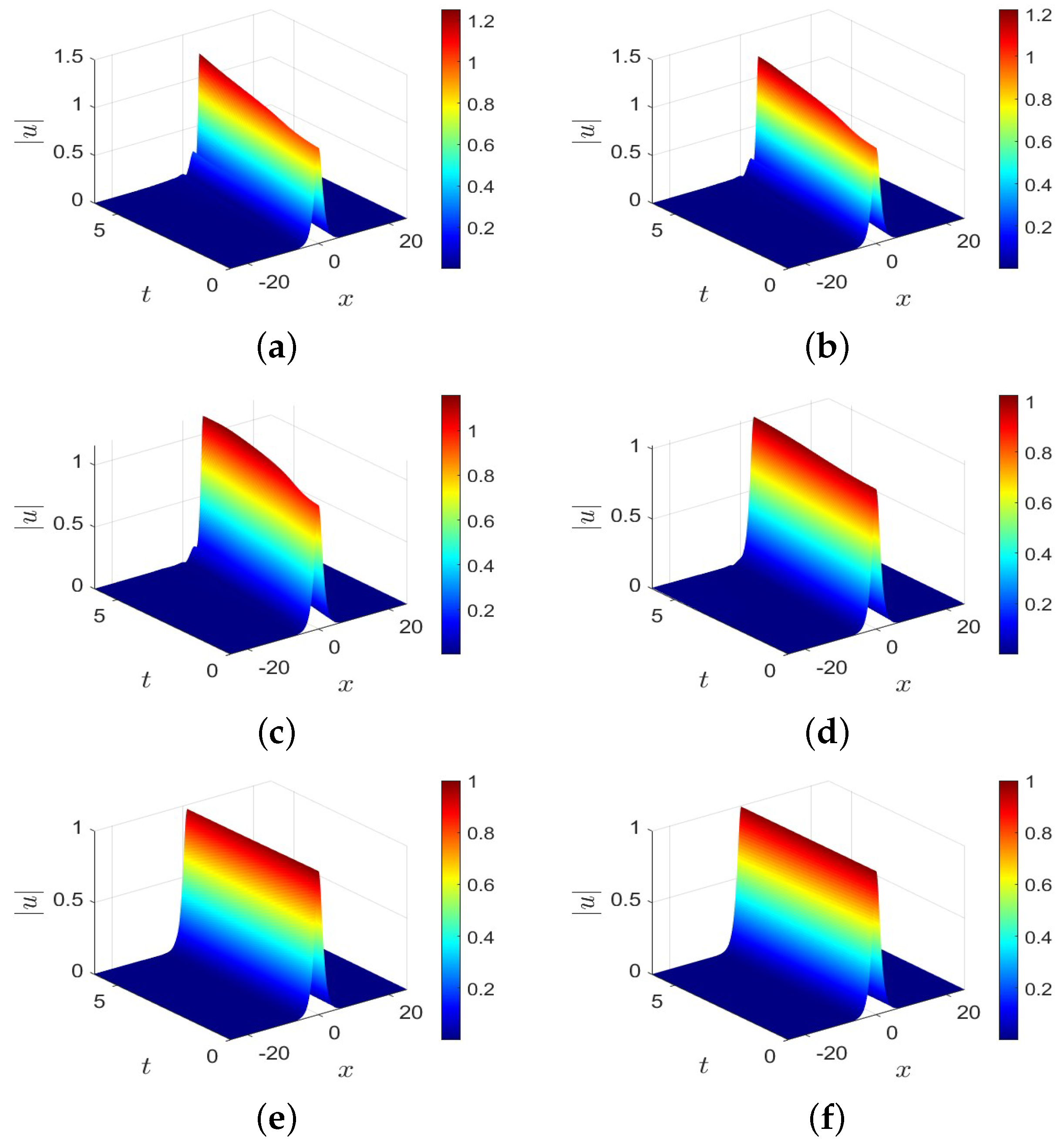
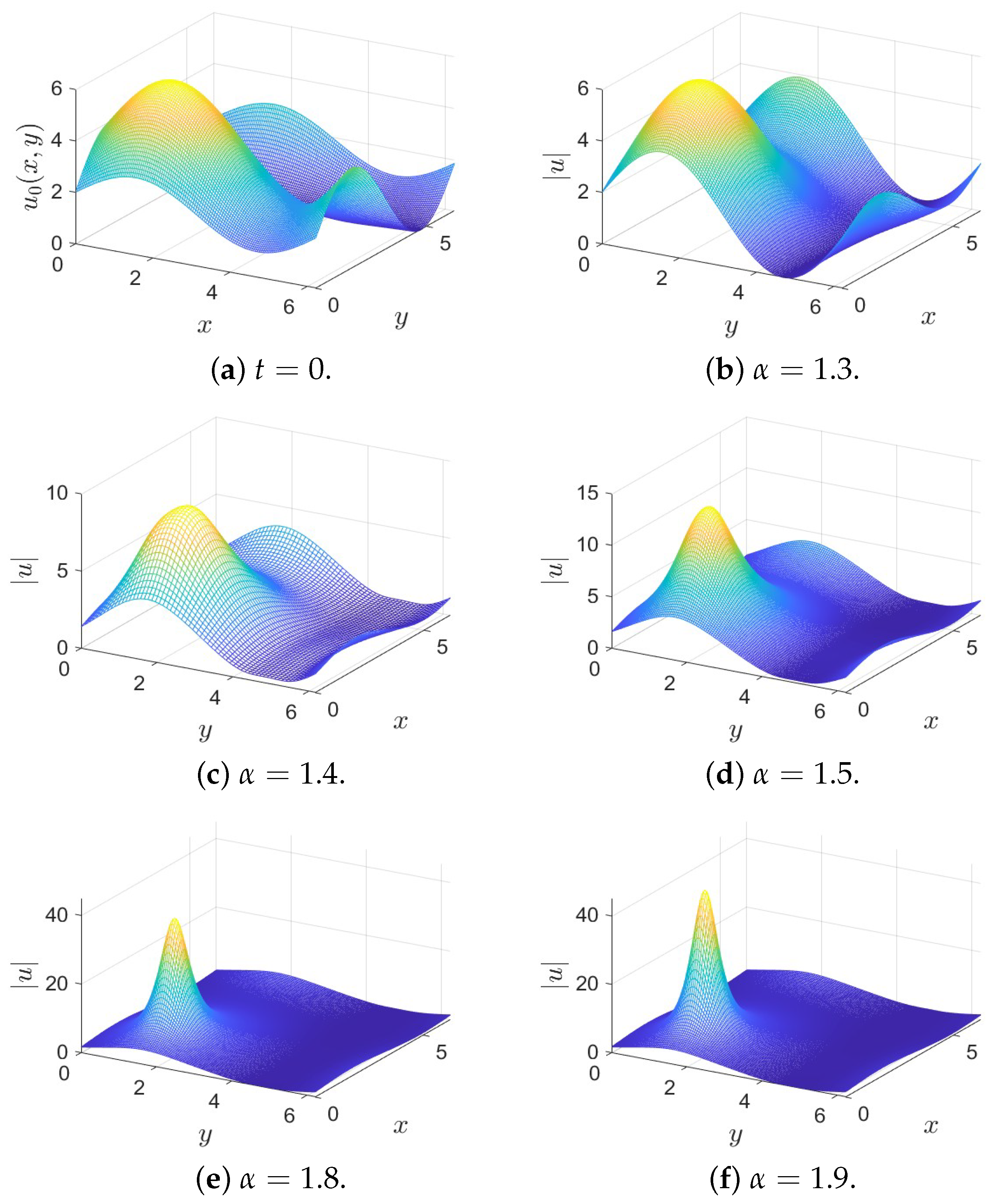
In Figure 1, the surfaces of the numerical solution $\left|u\right(x,t\left)\right|$ computed by SAV-WSLD-RRK methods with $\tau =1/2^9$ and $h=\pi /2^{10}$ are depicted for different values of order $\alpha$. We observe from Figure 1 that the values of order $\alpha$ affect the shape of the soliton. What is more, in Figure 2, we plot the numerical solutions $\left|u\right(x,t\left)\right|$ for Equation (24) for time $t=1,3,5$ for $\alpha =1.5,1.8$ with $\tau =1/2^9$ and $h=\pi /2^{10}$.

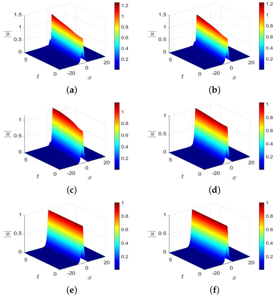
Figure 1. Surfaces of the numerical solutions $\left|u\right|$ of Equation (24) for different $\alpha$ with $\tau =1/2^9$ and $h=\pi /2^{10}$. (a) Numerical solution for $\alpha =1.1$; (b) numerical solution for $\alpha =1.2$; (c) numerical solution for $\alpha =1.3$; (d) numerical solution for $\alpha =1.5$; (e) numerical solution for $\alpha =1.7$; (f) numerical solution for $\alpha =2$.

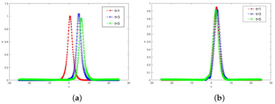
Figure 2. Numerical solutions for Equation (24) for time $t=1,3,5$ for different $\alpha$ with $\tau =1/2^9$ and $h=\pi /2^{10}$. (a) Numerical solution for time $t=1,3,5$ for $\alpha =1.5$; (b) numerical solution for time $t=1,3,5$ for $\alpha =1.8$.

It can be seen that there are two turning points. From Figure 1 and Figure 2, it can be observed that the shape of the soliton changes more rapidly as $\alpha$ decreases. As $\alpha$ approaches 2, the numerical solutions of the F-NLS Equation (24) converge to the exact solutions of the Integer-order Schrödinger equation.

To estimate the error and verify the convergence of the new methods, we define the discrete $L_2$-norm error of the numerical solution for the 1D problem as follows

$$\begin{array}{c}\hfill Erro{r}_h^{\tau }=\sqrt{\sum _{j=0}^{N_x-1}h{\left|U_j^M-u(x_j,T)\right|}^2},\end{array}$$

where $\left\{U_j^M|0\le j\le N_x-1\right\}$ is the numerical solution with time grid $\tau =T/M$ and space grid $h=(b-a)/N_x$ at time T, and $u(x_j,T)$ is the analytical solution for the F-NLS equations. However, most of the exact solutions of fractional differential equations are hard to obtain. For this reason, as in [35,36,37], the errors in the temporal and spatial directions can be computed by

$$\begin{array}{c}\hfill Erro{r}^{\tau }=\sqrt{\sum _{j=0}^{N_x-1}h{\left|U_j^M-U_j^{2M}\right|}^2},Erro{r}_h=\sqrt{\sum _{j=0}^{N_x-1}h{\left|U_j^M-U_{2j}^M\right|}^2},\end{array}$$

with sufficiently small h and $\tau$, respectively.

Then, the experimental order of convergence (EOC) can be calculated by

$$\begin{array}{c}\hfill EO{C}_{\tau }={\displaystyle \frac{{log}_2(Erro{r}^{{\tau }_1}/Erro{r}^{{\tau }_2})}{{log}_2({\tau }_1/{\tau }_2)}},EO{C}_h={\displaystyle \frac{{log}_2(Erro{r}_{h_1}/Erro{r}_{h_2})}{{log}_2(h_1/h_2)}},\end{array}$$

if h and $\tau$ are sufficiently small, respectively.

In Table 1, we verify the convergence orders in the temporal and spatial directions for the present method. Table 1 shows the errors at $T=1$ and the EOCs in temporal and spatial directions of Equation (24) with $\alpha =1.5$ and 2. We find that the present method, when using the second-order RRK method, exhibits an approximate second-order EOC in the temporal direction and is close to fourth-order in the spatial direction.

Table 1. The errors in the temporal and spatial directions and convergence orders of Equation (24) using the proposed method.

$\mathit{\alpha }$	$\mathit{\tau }$	h	$\mathit{E}\mathit{r}\mathit{r}\mathit{o}{\mathit{r}}_{\mathit{h}}$	$\mathit{E}\mathit{O}{\mathit{C}}_{\mathit{h}}$	h	$\mathit{\tau }$	$\mathit{E}\mathit{r}\mathit{r}\mathit{o}{\mathit{r}}^{\mathit{\tau }}$	$\mathit{E}\mathit{O}{\mathit{C}}_{\mathit{\tau }}$
1.5	$1/2^{10}$	$\pi /2^6$	$1.1991\times {10}^{-1}$	–	$\pi /2^9$	$1/2^5$	$5.2266\times {10}^{-2}$	–
		$\pi /2^7$	$7.9256\times {10}^{-3}$	3.9192		$1/2^6$	$1.2603\times {10}^{-2}$	2.0521
		$\pi /2^8$	$8.5764\times {10}^{-4}$	3.2081		$1/2^7$	$5.8514\times {10}^{-3}$	1.1069
		$\pi /2^9$	$5.3900\times {10}^{-5}$	3.9920		$1/2^8$	$1.8240\times {10}^{-3}$	1.6817
2	$1/{10}^3$	$\pi /2^6$	$4.0759\times {10}^{-2}$	–	$\pi /2^{10}$	$1/2^5$	$2.2878\times {10}^{-2}$	–
		$\pi /2^7$	$3.2603\times {10}^{-3}$	3.6440		$1/2^6$	$7.3454\times {10}^{-3}$	1.6390
		$\pi /2^8$	$1.6732\times {10}^{-4}$	4.2843		$1/2^7$	$2.9819\times {10}^{-3}$	1.3006
		$\pi /2^9$	$1.0642\times {10}^{-5}$	3.9748		$1/2^8$	$1.0803\times {10}^{-3}$	1.4648

Next, we verify the energy conservation property. To this end, we define the discrete energy error, $Erro{r}_{E\left(t_j\right)}=\left|E_{\gamma }^j-E_{\gamma }^0\right|/\left|E_{\gamma }^0\right|$, where $E_{\gamma }^j$ is defined in (22).

Figure 3 displays the discrete energy errors for Equation (24) with different fractional orders, $\alpha$, for time $t\in [0,6]$. It can be seen from Figure 3 that the proposed scheme preserves the energy at a discrete level, which coincides with Theorem 3 and Remark 3, and the energy error reaches the order of ${10}^{-3}$, which has a good conservation performance.

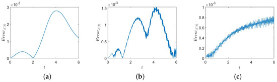
Figure 3. Energy errors for Equation (24) for time $t\in [0,6]$ for different $\alpha$ with $\tau =1/2^9$ and $h=\pi /2^{10}$. (a) Energy error for $\alpha =1.3$; (b) energy error for $\alpha =1.5$; (c) energy error for $\alpha =2$.

5.2. Two-Dimensional F-NLS Equation Problems

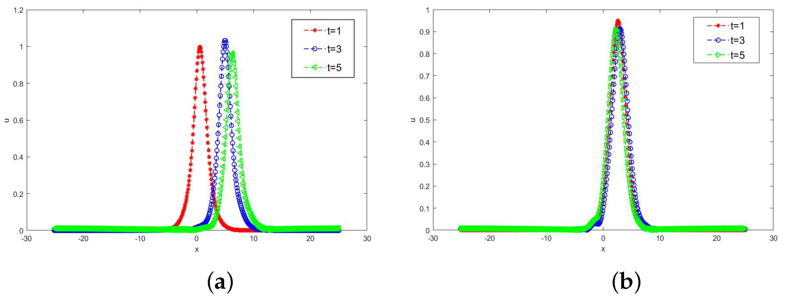
Firstly, we consider the following two-dimensional F-NLS equation problem [38]

$$\begin{array}{cc}\hfill & i{u}_t+{\displaystyle \frac{1}{2}}\left[{\left(-{△}_x\right)}^{{\displaystyle \frac{\alpha }{2}}}u+{\left(-{△}_y\right)}^{{\displaystyle \frac{\alpha }{2}}}u\right]+\rho {\left|u\right|}^{2}u=0,\left(x,y\right)\in D={\left[-20,20\right]}^2,t\in \left(0,T\right]\hfill \\ \hfill & u\left(x,y,t\right)=0,\left(x,y\right)\in \partial D,t\in \left[0,T\right],\hfill \\ \hfill & u\left(x,y,0\right)={\displaystyle \frac{2}{\sqrt{\pi }}}exp\left[-\left(x^2+y^2\right)\right],\left(x,y\right)\in D\cup \partial D.\hfill \end{array}$$

(26)

The numerical solutions $\left|u\right|$ of problem (26) with $\alpha =1.3,1.7,1.9$ and $\rho =2$ at time $t=0.3$ and $t=0.8$ obtained by the present numerical method are shown in Figure 4. It can be seen from Figure 4 that the wave peak lies at the origin of the coordinate plane, and that the amplitude of the wave will diminish with the extension of time. Moreover, from Figure 4, it also can be seen that the wave disperses faster for $\alpha =1.7,1.9$, than that for $\alpha =1.3$, i.e., the larger $\alpha$ is, the greater is the dispersion effect on the shape of the wave.

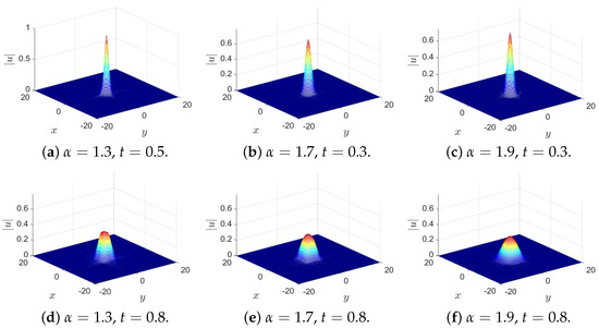
Figure 4. Numerical solutions $\left|u\right|$ of Equation (26) for different $\alpha$ at $t=0.3$ and $t=0.8$ using the present method with $\tau =1/100$ and $h=1/2^5$.

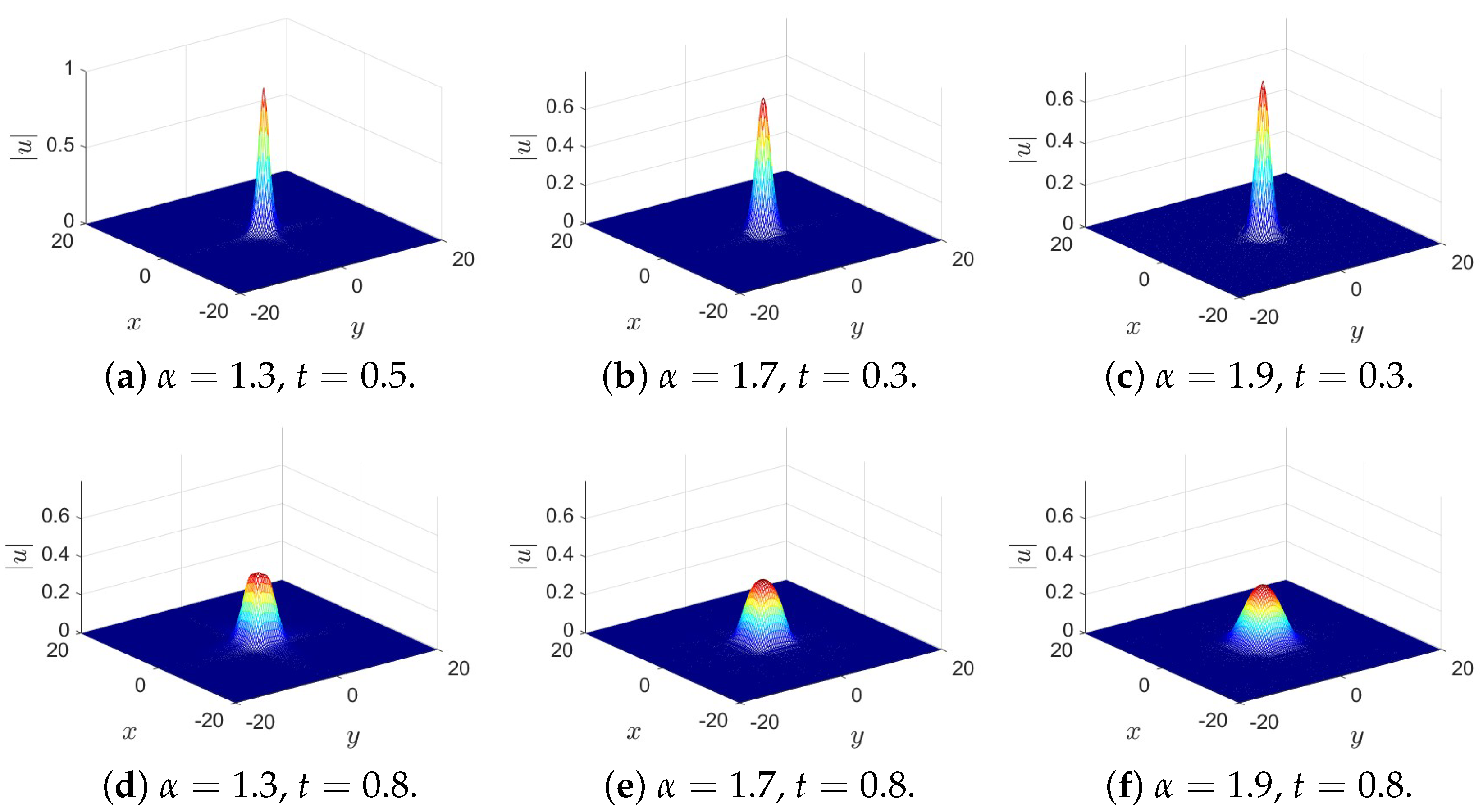
Secondly, we consider the following two-dimensional problem [39]

$$\begin{array}{cc}\hfill & i{u}_t+{\displaystyle \frac{1}{2}}\left[{\left(-{△}_x\right)}^{{\displaystyle \frac{\alpha }{2}}}u+{\left(-{△}_y\right)}^{{\displaystyle \frac{\alpha }{2}}}u\right]+\rho {\left|u\right|}^{2}u=0,\left(x,y\right)\in D={\left[0,2\pi \right]}^2,t\in \left(0,T\right],\hfill \\ \hfill & u\left(x,y,0\right)=\left(1+sinx\right)\left(2+siny\right),\left(x,y\right)\in D\cup \partial D,\hfill \end{array}$$

(27)

with periodic boundary conditions on $\partial D$.

The numerical solutions $\left|u\right|$ of problem (27) with $\alpha =1.3,1.4,1.5,1.8,1.9$ and $\rho =2$ at time $t=0.108$ obtained by the present numerical method are shown in Figure 5. It can be seen from Figure 5 that there is a singularity near the boundary occurring at $t=0.108$. Moreover, from Figure 5, it also can be seen that the singularity becomes weaker as $\alpha$ becomes smaller.

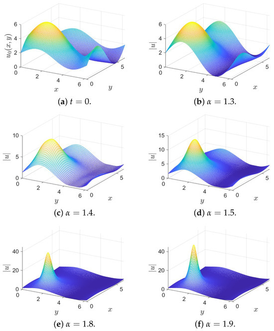
Figure 5. Numerical solutions $\left|u\right|$ of (27) for different $\alpha$ at $t=0.108$ using the present method with $\tau =1/100$ and $h=1/2^5$.

6. Conclusions

This paper presented an energy-preserving method for space F-NLS equations based on the SAV approach and RRK methods, in which the spatial direction is discretized by a fourth-order approximation. The energy conservation of the novel method is proven. Finally, the effectiveness and the conservation of the numerical method are verified by several numerical experiments in both one- and two-dimensional cases.

References

- Baleanu, D.; Karaca, Y.; Vázquez, L.; Macías-Díaz, J.E. Advanced fractional calculus, differential equations and neural networks: Analysis, modeling and numerical computations. Phys. Scr. 2023, 98, 110201. [Google Scholar] [CrossRef]
- Guo, X.; Xu, M. Some physical applications of fractional Schrödinger equation. J. Math. Phys. 2006, 47, 082104. [Google Scholar] [CrossRef]
- Muhammad, J.; Younas, U.; Nasreen, N.; Khan, A.; Abdeljawad, T. Multicomponent nonlinear fractional Schrödinger equation: On the study of optical wave propagation in the fiber optics. Partial. Differ. Equ. Appl. Math. 2024, 11, 100805. [Google Scholar] [CrossRef]
- Xu, Z.; Fu, Y. Two novel conservative exponential relaxation methods for the space-fractional nonlinear Schrödinger equation. Comput. Math. Appl. 2023, 142, 97–106. [Google Scholar] [CrossRef]
- Duo, S.; Zhang, Y. Mass-conservative Fourier spectral methods for solving the fractional nonlinear Schrödinger equation. Comput. Math. Appl. 2016, 71, 2257–2271. [Google Scholar] [CrossRef]
- Cheng, B.; Wang, D.; Yang, W. Energy preserving relaxation method for space-fractional nonlinear Schrödinger equation. Appl. Numer. Math. 2020, 152, 480–498. [Google Scholar] [CrossRef]
- Lischke, A.; Pang, G.; Gulian, M.; Song, F.; Glusa, C.; Zheng, X.; Mao, Z.; Cai, W.; Meerschaert, M.M.; Ainsworth, M.; et al. What is the fractional Laplacian? A comparative review with new results. J. Comput. Phys. 2020, 404, 109009. [Google Scholar] [CrossRef]
- Simos, T.; Williams, P. A finite-difference method for the numerical solution of the Schrödinger equation. J. Comput. Appl. Math. 1997, 79, 189–205. [Google Scholar] [CrossRef]
- Bao, W.; Cai, Y. Uniform error estimates of finite difference methods for the nonlinear Schrödinger equation with wave operator. SIAM J. Numer. Anal. 2012, 50, 492–521. [Google Scholar] [CrossRef]
- Karakashian, O.; Makridakis, C. A space-time finite element method for the nonlinear Schrödinger equation: The continuous Galerkin method. SIAM J. Numer. Anal. 1999, 36, 1779–1807. [Google Scholar] [CrossRef]
- Zhang, H.; Shi, D.; Li, Q. Nonconforming finite element method for a generalized nonlinear Schrödinger equation. Appl. Math. Comput. 2020, 377, 125141. [Google Scholar] [CrossRef]
- Thalhammer, M. Convergence analysis of high-order time-splitting pseudospectral methods for nonlinear Schrödinger equations. SIAM J. Numer. Anal. 2012, 50, 3231–3258. [Google Scholar] [CrossRef]
- Macías-Díaz, J.E. A structure-preserving method for a class of nonlinear dissipative wave equations with Riesz space-fractional derivatives. J. Comput. Phys. 2017, 351, 40–58. [Google Scholar] [CrossRef]
- Wang, P.; Huang, C. Structure-preserving numerical methods for the fractional Schrödinger equation. Appl. Numer. Math. 2018, 129, 137–158. [Google Scholar] [CrossRef]
- Macías-Díaz, J.E. An explicit dissipation-preserving method for Riesz space-fractional nonlinear wave equations in multiple dimensions. Commun. Nonlinear Sci. Numer. Simul. 2018, 59, 67–87. [Google Scholar] [CrossRef]
- Bai, G.; Hu, J.; Li, B. High-Order mass-and energy-conserving methods for the nonlinear Schrödinger equation. SIAM J. Sci. Comput. 2024, 46, A1026–A1046. [Google Scholar] [CrossRef]
- Hu, D.; Gong, Y.; Wang, Y. On convergence of a structure preserving difference scheme for two-dimensional space-fractional nonlinear Schrödinger equation and its fast implementation. Comput. Math. Appl. 2021, 98, 10–23. [Google Scholar] [CrossRef]
- Castillo, P.; Gómez, S. On the conservation of fractional nonlinear Schrödinger equation’s invariants by the local discontinuous Galerkin method. J. Sci. Comput. 2018, 77, 1444–1467. [Google Scholar] [CrossRef]
- Bhrawy, A.H.; Zaky, M. An improved collocation method for multi-dimensional space–time variable-order fractional Schrödinger equations. Appl. Numer. Math. 2017, 111, 197–218. [Google Scholar] [CrossRef]
- Zhai, S.; Wang, D.; Weng, Z.; Zhao, X. Error analysis and numerical simulations of Strang splitting method for space fractional nonlinear Schrödinger equation. J. Sci. Comput. 2019, 81, 965–989. [Google Scholar] [CrossRef]
- Wang, D.; Xiao, A.; Yang, W. A linearly implicit conservative difference scheme for the space fractional coupled nonlinear Schrödinger equations. J. Comput. Phys. 2014, 272, 644–655. [Google Scholar] [CrossRef]
- Liu, Y.; Ran, M. Arbitrarily high-order explicit energy-conserving methods for the generalized nonlinear fractional Schrödinger wave equations. Math. Comput. Simul. 2024, 216, 126–144. [Google Scholar] [CrossRef]
- Besse, C. A relaxation scheme for the nonlinear Schrödinger equation. SIAM J. Numer. Anal. 2004, 42, 934–952. [Google Scholar] [CrossRef]
- McLachlan, R. Featured review: Geometric numerical integration: Structure-preserving algorithms for ordinary differential equations. SIAM Rev. 2003, 45, 817–821. [Google Scholar]
- Leimkuhler, B.; Reich, S. Simulating Hamiltonian Dynamics; Number 14; Cambridge University Press: Cambridge, UK, 2004. [Google Scholar]
- Li, D.; Li, X.; Zhang, Z. Linearly implicit and high-order energy-preserving relaxation schemes for highly oscillatory Hamiltonian systems. J. Comput. Phys. 2023, 477, 111925. [Google Scholar] [CrossRef]
- Fu, Y.; Hu, D.; Wang, Y. High-order structure-preserving algorithms for the multi-dimensional fractional nonlinear Schrödinger equation based on the SAV approach. Math. Comput. Simul. 2021, 185, 238–255. [Google Scholar] [CrossRef]
- Sousa, E.; Li, C. A weighted finite difference method for the fractional diffusion equation based on the Riemann–Liouville derivative. Appl. Numer. Math. 2015, 90, 22–37. [Google Scholar] [CrossRef]
- Chen, M.; Deng, W. Fourth order accurate scheme for the space fractional diffusion equations. SIAM J. Numer. Anal. 2014, 52, 1418–1438. [Google Scholar] [CrossRef]
- Lubich, C. Discretized fractional calculus. SIAM J. Math. Anal. 1986, 17, 704–719. [Google Scholar] [CrossRef]
- Zhao, J.; Li, Y.; Xu, Y. An explicit fourth-order energy-preserving scheme for Riesz space fractional nonlinear wave equations. Appl. Math. Comput. 2019, 351, 124–138. [Google Scholar] [CrossRef]
- Li, Y.; Shan, W.; Zhang, Y. High-Order Dissipation-Preserving Methods for Nonlinear Fractional Generalized Wave Equations. Fractal Fract. 2022, 6, 264. [Google Scholar] [CrossRef]
- Ketcheson, D.I. Relaxation Runge–Kutta methods: Conservation and stability for inner-product norms. SIAM J. Numer. Anal. 2019, 57, 2850–2870. [Google Scholar] [CrossRef]
- Ranocha, H.; Sayyari, M.; Dalcin, L.; Parsani, M.; Ketcheson, D.I. Relaxation Runge–Kutta methods: Fully discrete explicit entropy-stable schemes for the compressible Euler and Navier–Stokes equations. SIAM J. Sci. Comput. 2020, 42, A612–A638. [Google Scholar] [CrossRef]
- Zhao, X.; Sun, Z.Z.; Hao, Z.P. A fourth-order compact ADI scheme for two-dimensional nonlinear space fractional Schrodinger equation. SIAM J. Sci. Comput. 2014, 36, A2865–A2886. [Google Scholar] [CrossRef]
- Weng, Z.; Zhuang, Q. Numerical approximation of the conservative Allen–Cahn equation by operator splitting method. Math. Methods Appl. Sci. 2017, 40, 4462–4480. [Google Scholar] [CrossRef]
- Willoughby, M.R. High-Order Time-Adaptive Numerical Methods for the Allen-Cahn and Cahn-Hilliard Equations. Ph.D. Thesis, University of British Columbia, Vancouver, BC, Canada, 2011. [Google Scholar]
- Wang, P.; Huang, C. Split-step alternating direction implicit difference scheme for the fractional Schrödinger equation in two dimensions. Comput. Math. Appl. 2016, 71, 1114–1128. [Google Scholar] [CrossRef]
- Liang, X.; Khaliq, A.Q. An efficient Fourier spectral exponential time differencing method for the space-fractional nonlinear Schrödinger equations. Comput. Math. Appl. 2018, 75, 4438–4457. [Google Scholar] [CrossRef]
Disclaimer/Publisher’s Note: The statements, opinions and data contained in all publications are solely those of the individual author(s) and contributor(s) and not of MDPI and/or the editor(s). MDPI and/or the editor(s) disclaim responsibility for any injury to people or property resulting from any ideas, methods, instructions or products referred to in the content. |
© 2024 by the authors. Licensee MDPI, Basel, Switzerland. This article is an open access article distributed under the terms and conditions of the Creative Commons Attribution (CC BY) license (https://creativecommons.org/licenses/by/4.0/).