Variational Bayesian Estimation of Quantile Nonlinear Dynamic Latent Variable Models with Possible Nonignorable Missingness

Abstract

Our study presents an innovative variational Bayesian parameter estimation method for the Quantile Nonlinear Dynamic Latent Variable Model (QNDLVM), particularly when dealing with missing data and nonparametric priors. This method addresses the computational inefficiencies associated with the traditional Markov chain Monte Carlo (MCMC) approach, which struggles with large datasets and high-dimensional parameters due to its prolonged computation times, slow convergence, and substantial memory consumption. By harnessing the deterministic variational Bayesian framework, we convert the complex parameter estimation into a more manageable deterministic optimization problem. This is achieved by leveraging the hierarchical structure of the QNDLVM and the principle of efficiently optimizing approximate posterior distributions within the variational Bayesian framework. We further optimize the evidence lower bound using the coordinate ascent algorithm. To specify propensity scores for missing data manifestations and covariates, we adopt logistic and probit models, respectively, with conditionally conjugate mean field variational Bayes for logistic models. Additionally, we utilize Bayesian local influence to analyze the Ecological Momentary Assessment (EMA) dataset. Our results highlight the variational Bayesian approach’s notable accuracy and its ability to significantly alleviate computational demands, as demonstrated through simulation studies and practical applications.

1. Introduction

Latent variable models are designed to estimate the relationships between observed variables and a hypothesized latent construct that is presumed to predict these variables. Dynamic latent variable models (DLVMs) extend this concept by accounting for unobserved heterogeneity through the explicit modeling of dependencies between observations and latent variables. This approach allows for the capture of variable effects across different spatial and temporal dimensions, providing a nuanced understanding of intra-individual dynamics and interindividual differences within ecological momentary assessments, as elucidated by Diener et al. [1] and Chow et al. [2]. Grasping the dynamic interplay and dependencies among latent and manifest variables over time is pivotal. Incorporating these lagged relationships is crucial for developing models that offer more profound insights and greater accuracy in explaining data patterns and trends. The exploration of lagged relationships among model elements is essential for crafting insightful models, which is why dynamic latent variable models have attracted considerable attention recently, as demonstrated by the works of Zhang et al. [3], Chow et al. [4] and Tang et al. [5]. However, the existing literature primarily assumes normality in directly measured error, which is especially susceptible to the influence of outliers and distributions characterized by heavy tails. To address this issue, a typical strategy is to relax the distributional constraints on variables that are directly measurable, focusing on their conditional quantiles instead of the full distribution, as explored by Wang et al. [6] and Tuerde et al. [7]. In our view, there is a sparse body of research concerning quantile nonlinear dynamic latent variable models (QNDLVMs). These models necessitate Markov chain Monte Carlo (MCMC) methods for inference, which can be computationally demanding and impractical for large datasets.

The cornerstone of empirical research is rooted in data collection and analysis, a process where missing values are an almost ubiquitous challenge. This issue spans across various fields, such as education, social sciences, and economics, due to factors like participants’ hesitancy to answer sensitive questions, accidental data loss, or withdrawal from studies (Little and Rubin [8]). Factor analysis with missing data has garnered significant interest from both theoretical researchers and practitioners. A multitude of methodologies have been developed for estimating strict latent variable models when data are incomplete. Banbura and Modugno [9], along with Jungbacker et al. [10], have explored likelihood estimation methods. For approximate factor models, Stock and Mark [11] suggest using the most recent estimate of the common component to fill in missing values in covariates. Despite differences in execution, a prevalent strategy is to utilize estimates from a balanced panel as starting values, as highlighted by Stock and Watson [12]. Recently, Tuerde et al. [7] developed a quantile nonlinear dynamic latent variable model to tackle missing data, but their approach is limited to continuous data and relies on MCMC techniques for inference. To overcome these constraints, we propose a variational Bayesian methodology capable of effectively managing nonignorable missing data.

Our inspiration comes from examining the data gathered through ecological momentary assessment (EMA) methods, as initially explored by Diener and colleagues in 1995. The research involved a group of 174 university students, consisting of 93 males and 81 females with an average age of 20.24 years and a standard deviation of 1.41 years. Participants were instructed to provide daily Ecological Momentary Assessment (EMA) ratings for various emotions using a seven-point Likert scale, with 1 representing “None” and 7 representing “Always”, over a period of 52 days. The directly measurable variables consist of eight ordinal scales: joy, contentment, love, affection, unphappiness, anger, depression, and anxiety. The top four scales are used to denote a latent positive emotion (PE), and the final four scales indicate a latent negative emotion (NE). The missing of data was not negligible; discrete variables are intertwined with individual beliefs and ethical considerations. The missing data made up about 11.2% of the entire dataset. This study seeks to investigate the evolving and nonlinear interactions between positive emotions (PE) and negative emotions (NE), with a particular focus on how these dynamics are affected by prior levels of emotions that possess opposing valences.

We present our innovative contributions: (i) We unveil a deterministic variational Bayesian approach designed to tackle nonlinear dynamic latent variable models (DLVMs), even when faced with the challenges of a nonparametric prior and possible nonignorable missingness data; (ii) To effectively manage nonignorable missing covariates and responses, we employ a set of univariate dimensional logistic and probit models, which facilitate optimizing evidence of the lower bound for robust statistical inference based on their respective posterior distributions; (iii) Our dynamic model benefits from the assumption of a Dirichlet prior for the random effects, offering reasonable representation of the underlying processes; (iv) We take Bayesian local influence analysis to new heights by conducting a comprehensive sensitivity analysis across multiple model components.

This article is organized in a systematic fashion. In Section 2, we begin by delineating the quantile regression model, proceed to elucidate the mechanisms and distributions associated with missing data, and culminate with an introduction to the Dirichlet process. Section 3 introduces a variational Bayesian methodology aimed at estimating the challenging parameters that have been estimated, random effects, and latent factor variables. Section 4 includes simulation studies that analyze the finite sample performance of these techniques. Section 5 illustrates the application of our methodologies through a real-world example. Finally, we conclude with a succinct discussion in Section 6.

2. Model

2.1. Quantile Nonlinear DLVM

A nonlinear dynamic latent variable model (DLVM) comprises two distinct submodels. The first submodel is a measurement model, which serves to elucidate the connections between latent factors and their corresponding variables that are directly observable. The second submodel is a dynamic model, applied to investigate the time-delayed interactions among latent variables. The measurement model that establishes the connection between latent variables and their associated variables that are directly observable is delineated as follows:

$${\mathit{z}}_{it}={\mathit{x}}_{it}\mathsf{\omega }+\mathsf{\Lambda }{\mathsf{\varphi }}_{it}+{\mathsf{\epsilon }}_{it},t=1,\dots ,T_i,i=1,\dots ,n,$$

(1)

where we encounter a vector of observable variables represented as $z_{it}={(z_{1it},\dots ,z_{Jit})}^{\top }$, which is continuous with a $J\times 1$ vector of variables that are directly observable. Concurrently, there is $x_{it}$, a $J\times K$ vector of covariates that may have missing data. We also introduce ${\mathsf{\varphi }}_{it}$, a $q\times 1$ vector that signifies hidden factors affecting our observations. The vector $\mathsf{\omega }$ contains the K regression coefficients, and $\mathsf{\Lambda }$ acts as the $J\times q$ matrix, capturing the interplay between our manifest and latent variables. Furthermore, ${\mathsf{\epsilon }}_{it}$ is a J-dimensional error term, which is uncorrelated with both $x_{it}$ and ${\mathsf{\varphi }}_{it}$. The sample size is denoted by n, and $T_i$ represents the number of repeated measurements for each individual observation. In some cases, we might encounter a scenario where $T_1=\dots =T_n$, which results in a balanced design. To move forward without losing any generality, let us set $T_1=T_2=\dots =T_n=T$ [4]. In the traditional framework of the dynamic latent variable model (DLVM), it is commonly accepted that the error term ${\mathsf{\epsilon }}_{it}$ adheres to a multivariate normal distribution. If the normality assumption for $z_i$ is violated, it may result in biased parameter estimates. Consequently, it is crucial to develop a more robust approach within the context of dynamic factor analysis. To tackle this issue, we will investigate the conditional quantile regression (QR) of $z_{jit}$ conditional on $x_{jit}$ and ${\mathsf{\varphi }}_{it}$ for a specific quantile level $\tau$, where $0<\tau <1$. Thus, we focus on the conditional quantile regression (QR) of variable $z_{jit}$ on $x_{jit}$ and ${\mathsf{\varphi }}_{it}$ for the quantile level $\tau \in (0,1)$:

$$Q_{\tau }\left(z_{jit}\right|x_{jit},{\mathsf{\varphi }}_{it})=x_{jit}^{\top }{\mathsf{\omega }}_{\tau }+{\mathsf{\Lambda }}_{\tau j}^{\top }{\mathsf{\varphi }}_{it},j=1,\dots ,J,i=1,\dots ,n,t=1,\dots ,T,$$

(2)

where the expression $Q_{\tau }\left(z_{jit}\right|x_{jit},{\mathsf{\varphi }}_{it})=\inf \{z:F\left(z\right|x_{jit},{\mathsf{\varphi }}_{it})\ge \tau \}$ represents the $\tau$th conditional quantile of $z_{jit}$ given the covariates $x_{jit}$ and the parameters ${\mathsf{\varphi }}_{it}$. Here, $F\left(z\right|x_{jit},{\mathsf{\varphi }}_{it})$ denotes the conditional cumulative distribution function of $z_{jit}$ based on the same covariates and parameters. The vectors $x_{jit}^{\top }$ and ${\mathsf{\Lambda }}_{\tau j}^{\top }$ correspond to the jth row of the matrices $x_{it}$ and ${\mathsf{\Lambda }}_{\tau }$, respectively. Additionally, $z_{jit}$ signifies the jth component of the vector $z_{it}$, while ${\mathsf{\omega }}_{\tau }$ is a regression coefficient with K-dimensions, and ${\mathsf{\Lambda }}_{\tau }$ is a $J\times q$ loading matrix of the latent factor associated with the quantile level $\tau$. It is important to note that both ${\mathsf{\omega }}_{\tau }$ and ${\mathsf{\Lambda }}_{\tau }$ may exhibit variability across different quantiles, indicating that distinct values of $\tau$ are associated with varying coefficients and loading matrices of the latent factors.

According to Kozumi et al. [13], the quantile regression model, denoted by Equation (2), can be re-expressed in the subsequent hierarchical models:

$$\left\{\begin{array}{c}{z}_{jit}=x_{jit}^{\top }{\mathsf{\omega }}_{\tau }+{\mathsf{\Lambda }}_{\tau j}^{\top }{\mathsf{\varphi }}_{it}+{\rho }_1{\nu }_{jit}+\sqrt{{\gamma }_j^{-1}{\rho }_2{\nu }_{jit}}{l}_{jit},\hfill \\ {\nu }_{jit}|{\gamma }_j\sim \mathrm{Exp}\left({\gamma }_j^{-1}\right)={\gamma }_{j}exp(-{\gamma }_j{\nu }_{jit}),\hfill \\ l_{jit}\sim \mathcal{N}(0,1)j=1,\dots ,J,i=1,\dots ,n,t=1,\dots ,T_i.\hfill \end{array}\right.$$

where the variable ${\nu }_{jit}$ follows an exponential distribution characterized by the parameter ${\gamma }_j^{-1}$, denoted as Exp(${\gamma }_j^{-1}$). The probability density function for ${\nu }_{jit}$ given ${\gamma }_j$ is expressed as $f\left({\nu }_{jit}\right|{\gamma }_j)={\gamma }_{j}exp(-{\gamma }_j{\nu }_{jit})$. Additionally, the variable $l_{jit}\sim \mathcal{N}(0,1)$. Furthermore, the parameters ${\rho }_1$ and ${\rho }_2$ are defined as follows: ${\rho }_1=(1-2\tau )/\left\{\tau (1-\tau )\right\}$ and ${\rho }_2=2/\left\{\tau (1-\tau )\right\}$.

The model, which operates on a dynamic basis, for investigating the ties among the latent variables is considered to be:

$${\mathsf{\varphi }}_{it}=f_t({\mathsf{\varphi }}_{i,t-1},{\mathsf{\mu }}_i,{\mathsf{\theta }}_{\varphi })+{\mathsf{\zeta }}_{it},{\mathsf{\zeta }}_{it}\stackrel{\mathrm{i}.\mathrm{i}.\mathrm{d}}{\sim }{\mathcal{N}}_q(0,{\mathsf{\Psi }}_{\zeta }),$$

(3)

In the model being proposed, the vector ${\mathsf{\mu }}_i$, with dimensions of $r\times 1$ encapsulates the random influences that are constant over time and unique to each individual. As a $q\times 1$ vector of functions that vary and are differentiable over time, $f_t(·)$ maps the interaction between the latent variables at time t and their levels one time unit earlier. The vector ${\mathsf{\theta }}_{\varphi }$ consists of parameters that are invariant across both time and individuals, while ${\mathsf{\Psi }}_{\zeta }$ denotes a $q\times q$ covariance matrix associated with ${\mathsf{\zeta }}_{it}$. In the standard dynamic models, it is a typical assumption that the ${\mathsf{\mu }}_i$ are independent and identically follow a multivariate normal distribution. Nevertheless, in certain cases [14], the presupposition of a normal distribution for the vector ${\mathsf{\mu }}_i$ may not be appropriate. To address this issue, we propose that ${\mathsf{\mu }}_i$ is drawn from an unknown distribution, specifically, ${\mathsf{\mu }}_i\sim \mathcal{G}$, The notation $\mathcal{G}$ here is meant to represent a probability distribution that is random and without a fixed form.

In order to conduct Bayesian analysis on the parameters $\mathsf{\mu }$, we employ a Dirichlet process (DP) prior to approximate the distribution $\mathcal{G}$. Specifically, we assume that $\mathcal{G}\sim \mathrm{DP}\left(\kappa G_0\right)$, where $G_0$ serves as a basic distribution that sets up a preliminary scaffold for an uncharted distribution. The parameter $\kappa$ is a positive constant that represents the probability assigned by the user to the base distribution $G_0$. The choice of $G_0$ is contingent upon the characteristics of the dataset under investigation.

In accordance with the methodologies established by Blei et al. [15], we make use of the stick-breaking technique to simulate the DP prior. Specifically, we articulate $\mathcal{G}\sim \mathrm{DP}\left(\kappa G_0\right)$ as

$$\mathcal{G}(·)=\sum _{s=1}^{\infty }{\pi }_s{\delta }_{U_s}(·),{\mathit{U}}_s\stackrel{\mathrm{i}.\mathrm{i}.\mathrm{d}}{\sim }{G}_0,$$

Here, we have the Dirac delta measure, denoted as ${\delta }_{U_s}(·)$, which is tightly focused on the vector ${\mathit{U}}_s$. This vector ${\mathit{U}}_s$ is an $r\times 1$ array that encapsulates the potential values of ${\mathsf{\mu }}_i$. The ${\pi }_s$ values represent random probability weights that adhere to the constraints of being between 0 and 1, with their total summing to 1 across all s from 1 to infinity. The structure of $\mathcal{G}$ suggests that it is created from a variety of point masses or elongated sticks with different lengths, each anchored at different points defined by ${\mathit{U}}_s$. To facilitate the sampling of observations, we delve into the concept of a truncated Dirichlet Process (DP) for $\mathcal{G}$:

$$\mathcal{P}(·)\approx \sum _{s=1}^S{\pi }_s{\delta }_{U_s}(·),{\mathit{U}}_s\stackrel{\mathrm{i}.\mathrm{i}.\mathrm{d}}{\sim }{G}_0,1\le S<\infty ,$$

(4)

where the ${\pi }_s$ values are set by the stick-breaking strategy presented below:

$${\pi }_1=v_1,{\pi }_s=v_s\prod _{l<s}(1-v_l)\mathrm{for}s=2,\dots ,S,$$

(5)

with $v_s\sim \mathrm{beta}(1,\mathrm{b})$ for $s=1,\dots ,S-1$, $v_S=1$ and ${\sum }_{s=1}^S{\pi }_s=1$.

Given the presence of some complex posterior distributions, optimizing the posterior distribution of ${\mathsf{\mu }}_i$ using the previously defined DP prior through a variational Bayesian approach is not feasible. To tackle this challenge, we define ${\mathsf{\mu }}_i$ in relation to a latent variable ${\mathcal{L}}_i\in 1,\dots ,S$, which tracks the cluster affiliation of each ${\mathsf{\mu }}_i$ and correlates with ${\mathsf{\mu }}_i$ through ${\mathsf{\mu }}_i={\mathit{U}}_{{\mathcal{L}}_i}$. Consequently, Equation (4) can be reformulated as:

$${\mathcal{L}}_i|\mathsf{\pi }\stackrel{\mathrm{i}.\mathrm{i}.\mathrm{d}}{\sim }\sum _{s=1}^S{\pi }_s{\delta }_{Us}(·),$$

(6)

where $\mathsf{\pi }={({\pi }_1,\dots ,{\pi }_S)}^{\top }$.

2.2. Mechanism of Missing Data

In this study, we acknowledge that both $z_{it}$ and $x_{jit}$ may have some missing values in their data. We can break down ${\mathbf{z}}_{it}$ into two parts: the observed data, ${\mathbf{z}}_{it,\mathrm{obs}}$, and the missing data, ${\mathbf{z}}_{it,\mathrm{mis}}$. Similarly, for $x_{jit}$, we have the observed portion, $x_{jit,\mathrm{obs}}$, and the missing portion, $x_{jit,\mathrm{mis}}$. This distinction allows us to clearly identify which data points we have and which ones are still elusive. Let ${\mathit{r}}_{it}^z={(r_{1it}^z,\dots ,r_{Jit}^z)}^{\top }$ be a vector of missing indicators for $z_{it}$ which has dimensions $J\times 1$, i.e., $r_{kit}^z=0$ if $z_{kit}$ is missing and $r_{kit}^z=1$ if $z_{kit}$ is observed for $k=1,\dots ,J$. Likewise, we establish $r_{jit}^x={(r_{jit,1}^x,\dots ,r_{jit,n_k}^x)}^{\top }$ to represent the missing data indicator for $x_{jit}$, with $r_{jit,k}^x=0$ indicating missing data for $x_{jit,k}$, and $r_{jit,k}^x=1$ indicating observed data. To streamline notation, we define $f\left(r_{it}^z\right|z_{it},\mathsf{\chi })$ and $f\left(r_{jit}^x\right|x_{jit},\mathsf{\xi })$ as the probability density functions for $r_{it}^z$ and $r_{jit}^x$, respectively, Here, $\mathsf{\chi }$ and $\mathsf{\xi }$ represent the parameter vectors linked to the missing data indicators $r_{it}^z$ and $r_{jit}^x$.

Given that $r_{git}^z$ is independent of $r_{hit}^z$ for $g\ne h$, owing to the binary nature of $r_{kit}^z$, we consider the following model: $f\left(r_{it}^z\right|z_{it},\mathsf{\chi })$:

$$f\left({\mathit{r}}_{it}^z\right|{\mathbf{z}}_{it},\mathsf{\chi })=\prod _{k=1}^J{\left\{\mathrm{Pr}(r_{kit}^z=1|{\mathbf{z}}_{it},\mathsf{\chi })\right\}}^{r_{kit}^z}{\{1-\mathrm{Pr}(r_{kit}^z=1|{\mathbf{z}}_{it},\mathsf{\chi })\}}^{1-r_{kit}^z},$$

where the probability $\mathrm{Pr}(r_{kit}^z=1|{\mathbf{z}}_{it},\mathsf{\chi })$ is contingent upon the missing entries in $z_{it}$, signifying that the mechanism of data missingness under consideration is not random, that is, it is nonignorable. Drawing parallels with the work of Tuerde et al. [7], through the use of a collection of univariate dimensional conditional probability distributions, we can detail the mechanism underlying the patterns of missing data within the model for $f\left(r_{jit}^x\right|x_{jit},\mathsf{\xi })$, That is to say

$$\begin{array}{ccc}f\left({\mathit{r}}_{jit}^x\right|{\mathit{x}}_{jit},\mathsf{\xi })\hfill & =\hfill & f\left(r_{jit,n_k}^x\right|{\mathit{r}}_{jit\left(n_k\right)}^x,{\mathit{x}}_{jit\left(n_k\right)},{\mathsf{\xi }}_{n_k})f\left(r_{jit,n_k-1}^x\right|{\mathit{r}}_{jit(n_k-1)}^x,{\mathit{x}}_{jit(n_k-1)},{\mathsf{\xi }}_{n_k-1})\hfill \\ \hfill & \hfill & \times \cdots \times f\left(r_{jit,2}^x\right|r_{jit\left(2\right)}^x,{\mathit{x}}_{jit\left(2\right)},{\mathsf{\xi }}_2)f\left(r_{jit,1}^x\right|x_{jit,1},{\mathsf{\xi }}_1),\hfill \end{array}$$

(7)

where ${\mathsf{\xi }}_k$ represents an unknown parameter vector linked to the conditional distribution of $r_{jit,k}^x$, conditioned on the set $\{{\mathit{r}}_{jit\left(k\right)}^x,{\mathit{x}}_{jit\left(k\right)}\}$, where ${\mathit{r}}_{jit\left(k\right)}^x=\{r_{jit,1}^x,\dots ,r_{jit,k-1}^x\}$ and ${\mathit{x}}_{jit\left(k\right)}=\{x_{jit,1},\dots ,x_{jit,k}\}$. Here, $x_{jit,k}$ denotes the element of $x_{jik}$ for $k=1,\dots ,n_k$, and $\mathsf{\xi }=\{{\mathsf{\xi }}_1,\dots ,{\mathsf{\xi }}_{n_k}\}$. Considering $r_{jit,k}^x$ as a binary indicator, it follows that:

$$\begin{array}{ccc}f\left(r_{jit,k}^x\right|r_{jit\left(k\right)}^x,x_{jit\left(k\right)},{\mathsf{\xi }}_k)\hfill & =\hfill & {\left\{\mathrm{Pr}(r_{jit,k}^x=1|r_{jit\left(k\right)}^x,x_{jit\left(k\right)},{\mathsf{\xi }}_k)\right\}}^{r_{jit,k}^x}\hfill \\ & & \times {\{1-\mathrm{Pr}(r_{jit,k}^x=1|r_{jit\left(k\right)}^x,x_{jit\left(k\right)},{\mathsf{\xi }}_k)\}}^{1-r_{jit,k}^x},\hfill \end{array}$$

Here, the probability $\mathrm{Pr}(r_{jit,k}^x=1|r_{jit\left(k\right)}^x,x_{jit\left(k\right)},{\mathsf{\xi }}_k)$ s influenced by the missing entries within $x_{jit}$, suggesting that the data’s missingness mechanism being examined is not ignorable.

In line with the research conducted by Lee and Tang [16], the likelihood Pr$(r_{kit}^z=1|{\mathbf{z}}_{it},\mathsf{\chi })$ can be delineated as

$$\mathrm{logit}\left\{\mathrm{Pr}(r_{kit}^z=1|{\mathbf{z}}_{it},\mathsf{\chi })\right\}={\chi }_{z0}+{\chi }_{z1}{z}_{kit}+{\chi }_{z2}{z}_{ki,t-1},k=1,\dots ,J,$$

where $\mathsf{\chi }={({\chi }_{z0},{\chi }_{z1},{\chi }_{z2})}^{\top }$ is a vector of the regression coefficients that are independent of both time and individual factors. In certain scenarios, it is plausible to account for a time-varying mechanism affecting data missingness. Consequently, an analogous model can be applied to determine $\mathrm{Pr}(r_{jit,k}^x=1|{\mathit{r}}_{jit\left(k\right)}^x,{\mathit{x}}_{jit\left(k\right)},{\mathsf{\eta }}_k)$; following Tuerde et al. [7], we define $\mathrm{Pr}(r_{jit,k}^x=1|{\mathit{r}}_{jit\left(k\right)}^x,{\mathit{x}}_{jit\left(k\right)},{\mathsf{\eta }}_k)$ using the probit regression model:

$${\Phi }^{-1}\left\{\mathrm{Pr}(r_{jit,k}^x=1|{\mathit{r}}_{jit\left(k\right)}^x,{\mathit{x}}_{jit\left(k\right)},{\mathsf{\eta }}_k)\right\}={\mathit{f}}_{jit,k}^{\top }{\mathsf{\eta }}_k,$$

(8)

where $f_{jit,k}={(1,x_{jit,1},\dots ,x_{jit,k},r_{jit,1}^x,\dots ,r_{jit,k-1}^x)}^{\top }$; the ${\Phi }^{-1}(·)$ denotes the standard normal CDF’s inverse transformation. To establish a foundational normal regression framework, we introduce latent variables. Specifically, by defining the latent variables ${\varsigma }_{jit,k}$, $(j=1,\dots ,J,$ $i=1,\dots ,n,$ and $t=1,\dots ,T,k=1,\dots ,n_k)$, model (8) can be rewritten as

$$r_{jit,k}^x=\left\{\begin{array}{ccc}\hfill 1& & \mathrm{if}{\varsigma }_{jit,k}>0,\hfill \\ \hfill 0& & \mathrm{if}{\varsigma }_{jit,k}\le 0,\hfill \end{array}\right.$$

(9)

where ${\varsigma }_{jit,k}={\mathit{f}}_{jit,k}^{\top }{\mathsf{\eta }}_k+{ϵ}_{jit,k},{ϵ}_{jit,k}\sim \mathcal{N}(0,1)$.

Drawing from Equation (9), the conditional probability density function as $r_{jit,k}^x$ given $\{{\mathit{r}}_{jit\left(k\right)}^x,{\mathit{x}}_{jit\left(k\right)}\}$ can be characterized by the expression

$$\begin{array}{ccc}f\left(r_{jit,k}^x\right|{\mathit{r}}_{jit\left(k\right)}^x,{\mathit{x}}_{jit\left(k\right)},{\mathsf{\eta }}_k)\hfill & =\hfill & \int f(r_{jit,k}^x,{\varsigma }_{jit,k}|{\mathit{r}}_{jit\left(k\right)}^x,{\mathit{x}}_{jit\left(k\right)},{\mathsf{\eta }}_k)d{\varsigma }_{jit,k}\hfill \\ & =\hfill & \int f\left({\varsigma }_{jit,k}\right|{\mathit{r}}_{jit\left(k\right)}^x,{\mathit{x}}_{jit\left(k\right)},{\mathsf{\eta }}_k)\{I(r_{jit,k}^x=1)I({\varsigma }_{jit,k}>0)\hfill \\ & & +I(r_{jit,k}^x=0)I({\varsigma }_{jit,k}\le 0)\}d{\varsigma }_{jit,k},\hfill \end{array}$$

where $f\left({\varsigma }_{jit,k}\right|{\mathit{r}}_{jit\left(k\right)}^x,{\mathit{x}}_{jit\left(k\right)},{\mathsf{\eta }}_k)\sim \mathcal{N}(f_{jit,k}^{\top }{\mathsf{\eta }}_k,1)$.

2.3. The Missing Covariates Distribution

Adhering to the methodology of Tuerde et al. [7], the joint density function can be derived by linking a chain of the forthcoming univariate dimensional conditional distributions $f\left({\mathit{x}}_{jit}\right|\mathsf{\beta },\mathsf{\delta })$:

$$f\left({\mathit{x}}_{jit}\right|\mathsf{\beta },\mathsf{\delta })=f\left(x_{jit,n_K}\right|x_{jit,1},\dots ,x_{jit,n_{K-1}},{\mathsf{\beta }}_{n_K},{\delta }_{n_K})\cdots f\left(x_{jit,2}\right|x_{jit,1},{\mathsf{\beta }}_2,{\delta }_2)f\left(x_{jit,1}\right|{\mathsf{\gamma }}_1,{\delta }_1),$$

(10)

where ${\mathsf{\gamma }}_k$ and ${\delta }_k$ can be estimated and linked to the k-th conditional distribution $f\left(x_{jit,k}\right|x_{jit,1}$, $\dots ,x_{jit,k-1},{\mathsf{\beta }}_k,{\delta }_k)$, $\mathsf{\beta }=\{{\mathsf{\beta }}_1,\dots ,{\mathsf{\beta }}_K\}$, and $\mathsf{\delta }=\{{\delta }_1,\dots ,{\delta }_K\}$. Equation (10) demonstrates flexibility in defining the distribution of covariates with missing data, irrespective of whether they are discrete random variables or continuous random variables. To allow for a broader range of distributions, it is posited that the missing covariate $x_{jit,k}(j=1,\dots ,J,i=1,\dots ,n$ and $t=1,\dots ,T,k=1,\dots ,n_K$) conforms to a distribution within the exponential family:

$$f\left(x_{jit,k}\right|x_{jit,1},\dots ,x_{jit,k-1},{\mathsf{\beta }}_k,{\delta }_k)=exp\left\{{\displaystyle \frac{x_{jit,k}{\vartheta }_{jit,k}-b_k\left({\vartheta }_{jit,k}\right)}{a_k\left({\delta }_k\right)}}-h_k(x_{jit,k},{\delta }_k)\right\},$$

(11)

where the functions $a_k(·)>0$ are strictly positive, while $b_k(·)$ and $h_k(·)$ are predetermined functions. The probability density function $x_{jit,k}$, as delineated in Equation (11), encompasses special instances such as the binomial distribution, Gaussian distribution, and gamma distribution. We give thought to the following model for ${\mu }_{jit,k}^x$:

$${\xi }_{jit,k}=g\left({\mu }_{jit,k}^x\right)={\beta }_{k0}+{\beta }_{k1}{x}_{jit,1}+\dots +{\beta }_{k,k-1}{x}_{jit,k-1},$$

where the link function $g(·)$ is identified and is strictly monotonically increasing, with differentiable attributes, and ${\mathsf{\beta }}_k={({\beta }_{k0},{\beta }_{k1},\dots ,{\beta }_{k,k-1})}^{\top }$.

3. Variational Bayesian Inference

Variational Bayes

For ease of understanding, we refer to $\mathsf{\Xi }=\{{\mathsf{\Xi }}_z,{\mathsf{\Xi }}_{\varphi },{\mathsf{\Psi }}_{\zeta },b,\kappa ,\mathsf{\gamma },\mathsf{\chi },\mathsf{\xi },\mathsf{\beta },\mathsf{\nu },\mathsf{\eta },{\mathsf{\mu }}_{\mu },{\mathsf{\Psi }}_{\mu },\mathsf{\varsigma },\mathcal{L}\}$, $r=\{r_z,r_x\}$, and $D_{\mathrm{obs}}=\{z_{\mathrm{obs}},x_{\mathrm{obs}},S\}$, in which ${\mathsf{\Xi }}_z$ encompasses all the parameters that are unknown and related to ${\mathsf{\omega }}_{\tau }$, ${\mathsf{\Lambda }}_{\tau }$ and $\mathsf{\gamma }=\{{\gamma }_1,\dots ,{\gamma }_p\}$, $r_x=\{r_{mit}^x:m=1,\dots ,M,i=1,\dots ,n,t=1,\dots ,T\}$, $r_z=\{r_{it}^z:i=1,\dots ,n,t=1,\dots ,T\}$, $z_{\mathrm{obs}}=\{z_{it,\mathrm{obs}}:i=1,\dots ,n,t=1,\dots ,T\}$, $x_{\mathrm{obs}}=\{x_{mit,\mathrm{obs}}:m=1,\dots ,M,i=1,\dots ,n,t=1,\dots ,T\}$, $S=\{S_{it}:i=1,\dots ,n,t=1,\dots ,T\}$, $\mathcal{L}=\{{\mathcal{L}}_i:i=i=1,\dots ,n\}$, $\mathsf{\varsigma }=\{{\varsigma }_{mit,k}:m=1,\dots ,M,i=1,\dots ,n,t=1,\dots ,T,k=1,\dots ,n_K\}$, $\mathit{D}=\{\mathit{x},\mathbf{z}\}$, ${\mathit{D}}_{obs}=\{{\mathit{x}}_{obs},{\mathbf{z}}_{obs}\}$; in light of the assumption stated above, the integrated posterior density of $\mathsf{\Xi }$ considering r and $D_{\mathrm{obs}}$, assumes the subsequent form

$$\begin{array}{ccc}f\left(\mathsf{\Xi }\right|r,D_{\mathrm{obs}})\hfill & \propto \hfill & \left\{{\displaystyle \prod _{i=1}^n}{\displaystyle \prod _{t=1}^T}\int f\left(z_{it}\right|x_{it},{\mathsf{\varphi }}_{it},{\mathsf{\nu }}_{it},{\mathsf{\Xi }}_z)f\left({\mathsf{\nu }}_{it}\right|\mathsf{\gamma })f\left({\mathsf{\varphi }}_{it}\right|{\mathsf{\mu }}_i,{\mathsf{\Xi }}_{\varphi },{\mathsf{\Psi }}_{\zeta })f\left({\mathsf{\mu }}_i\right|{\mathsf{\Xi }}_{\mu })f\left({\mathsf{\Psi }}_i\right|{\mathsf{\Xi }}_{\mu })\right.\hfill \\ & & f\left(x_{it,\mathrm{mis}}\right|\mathsf{\gamma },\mathsf{\varphi })f\left(r_{it}^z\right|z_{it},\mathsf{\chi })f\left(r_{it}^x\right|x_{it},\mathsf{\varsigma },\mathsf{\xi })f\left(\mathsf{\varsigma }\right|x,r_x,\mathsf{\psi })f\left(\mathsf{\chi }\right|{\mathbf{z}}_{obs,{\mathit{r}}_{it}^z})f\left(\mathsf{\xi }\right|{\mathbf{z}}_{obs,{\mathit{r}}_{it}^z})\hfill \\ & & \left.f\left(\kappa \right|\mathsf{\nu })f\left(\mathcal{L}\right|\mathsf{\pi })d{z}_{it,\mathrm{mis}}d{x}_{it,\mathrm{mis}}d{\mathsf{\varphi }}_{it}d{\mathsf{\nu }}_{it}d{\mathsf{\mu }}_{i}d\mathsf{\xi }d\mathsf{\chi }d\mathsf{\varsigma }\right\}f\left(\mathsf{\Xi }\right),\hfill \end{array}$$

where $x_{it,\mathrm{mis}}=\{x_{mit,\mathrm{mis}}:m=1,\dots ,M,i=1,\dots ,n,t=1,\dots ,T\}$, ${\mathsf{\nu }}_{it}=\{{\nu }_{mit}:m=1,\dots ,M,i=1,\dots ,n,t=1,\dots ,T\}$, $r_{it}^x=\{r_{mit}^x:m=1,\dots ,M,i=1,\dots ,n,t=1,\dots ,T\}$, ${\mathsf{\Xi }}_{\mu }$ is a parameter set related to the distribution of ${\mathsf{\mu }}_i$, $f\left(\mathsf{\Xi }\right)$ denotes the prior distribution of $\mathsf{\Xi }$. Obviously, the task of obtaining a closed-form representation of $f\left(\mathsf{\Xi }\right|r,D_{\mathrm{obs}})$ is quite arduous, given the intricate high-dimensional integrals at play, suggesting that Bayesian inference on $\mathsf{\Xi }$ is predicated on $f\left(\mathsf{\Xi }\right|r,D_{\mathrm{obs}})$. Addressing this issue, augmenting the sets $\{z_{\mathrm{mis}},x_{\mathrm{mis}},{\mathsf{\Xi }}_{\varphi },{\mathsf{\Psi }}_{\zeta },b,\kappa ,\mathsf{\nu },\mathsf{\chi },\mathsf{\xi },\mathsf{\beta },\mathsf{\varphi },{\mathsf{\mu }}_{\mu },{\mathsf{\Psi }}_{\mu },\mathsf{\varsigma },\mathcal{L}\}$ with the observed data $\{r,D_{\mathrm{obs}}\}$ in the Bayesian analysis facilitates the estimation of the posterior density $f\left(\mathsf{\Xi }\right|{\mathit{D}}_{obs},\mathit{r})$ that is conducive to Bayesian inference without the complexity of high-dimensional integrals.

According to the principles of variational inference, the initial step involves creating a variational family $\Omega$ of probability density functions for the random variable ℜ, which is designed to have the same support as the posterior distribution $g\left(\mathcal{\Re }\right|D)$, where $\mathsf{\Re }=\{{\mathsf{\Xi }}_z,{\mathsf{\Xi }}_{\varphi },{\mathsf{\Psi }}_{\zeta },b,\mathsf{\eta },\mathsf{\gamma },\mathsf{\chi },\mathsf{\xi },\mathsf{\varphi },{\mathsf{\mu }}_{\mu },{\mathsf{\Psi }}_{\mu },\mathsf{\nu },\mathsf{\varsigma },\mathcal{L}\}$. It is thought that $d\left(\mathsf{\Re }\right)$, which is in $\Omega$, is a variational density for approximating $g\left(\mathsf{\Re }\right|D)$. The variational Bayes strategy aims to identify the most fitting approximation to $g\left(\mathsf{\Re }\right|D)$ by minimizing the Kullback–Leibler divergence between $d\left(\mathsf{\Re }\right)$ and $g\left(\mathsf{\Re }\right|D)$, tackling the optimization problem:

$$d^{*}\left(\mathsf{\Re }\right)=\underset{d\left(\mathsf{\Re }\right)\in \Omega }{argmin}KL(d\left(\mathsf{\Re }\right)\parallel g\left(\mathsf{\Re }\right|D)),$$

where

$$\begin{array}{ccc}KL\left(d\right(\mathsf{\Re })\parallel g(\mathsf{\Re }\left|D\right))\hfill & =\hfill & \int log\left\{{\displaystyle \frac{d\left(\mathsf{\Re }\right)}{g\left(\mathsf{\Re }\right|D)}}\right\}\hfill \\ & =\hfill & \int log\{{\displaystyle \frac{d\left(\mathsf{\Re }\right)g\left(z\right|x)}{g(\mathsf{\Re },z|x)}}\}d\left(\mathsf{\Re }\right)d\mathsf{\Re }\hfill \\ & =\hfill & E_{d\left(\mathsf{\Re }\right)}\{logd\left(\mathsf{\Re }\right)\}-E_{d\left(\mathsf{\Re }\right)}\{logg(\mathsf{\Re },z|x)\}+logg\left(z\right|x)\ge 0\hfill \end{array}$$

where the term $E_{d\left(\mathsf{\Re }\right)}(·)$ in this case refers to the expected value relative to $d\left(\mathsf{\Re }\right)$. The Kullback–Leibler divergence $KL\left(d\right(\mathsf{\Re }\left)\right|g\left(\mathsf{\Re }\right|D\left)\right)$ is zeroed out if, and only if, $d\left(\mathsf{\Re }\right)$ is equivalent to $g\left(\mathsf{\Re }\right|D)$. The optimization problem is very difficult due to the complex high-dimensional integral.

Alternatively, it is demonstrated from $\mathrm{L}\left\{d\left(\mathsf{\Re }\right)\right\}=E_{d\left(\mathsf{\Re }\right)}\{logg(\mathsf{\Re },z|x)\}-E_{d\left(\mathsf{\Re }\right)}\{logd\left(\mathsf{\Re }\right)\}$ that

$$logg\left(\mathbf{z}\right|\mathit{x})=KL(d\left(\mathsf{\Re }\right)\parallel g\left(\mathsf{\Re }\right|D\left)\right)+\mathrm{L}\left\{d\right(\mathsf{\Re }\left)\right\}\ge \mathrm{L}\left\{d\right(\mathsf{\Re }\left)\right\}.$$

Therefore, ℜ is considered to be the minimum achievable value for $logg\left(\mathbf{z}\right|\mathit{x})$, commonly known as the Evidence Lower Bound (ELB) (see Appendix A). Following this, minimizing the Kullback–Leibler divergence $KL\left(d\right(\mathsf{\Re }\left)\right|g\left(\mathsf{\Re }\right|D\left)\right)$ is the same as maximizing $\mathrm{L}\left\{d\right(\mathsf{\Re }\left)\right\}$, because $logg\left(\mathbf{z}\right|\mathit{x})$ is not associated with ℜ. This means that,

$$d^{*}=\underset{d\left(\mathsf{\Re }\right)\in \Omega }{argmin}KL(d\left(\mathsf{\Re }\right)\parallel g\left(\mathsf{\Re }\right|D))=\underset{d\left(\mathsf{\Re }\right)\in \Omega }{argmax}\mathrm{L}\left\{d\left(\mathsf{\Re }\right)\right\}.$$

The goal of identifying the closest approximation to $g\left(\mathsf{\Re }\right|\mathit{D})$ becomes an issue of maximizing the problem of $\mathrm{L}\left\{d\right(\mathsf{\Re }\left)\right\}$ within the variational family $\Omega$. Due to the complexity inherent in the variational set $\Omega$, the optimization task becomes particularly challenging. As such, it is more reasonable to pursue optimization over a simpler variational set $\Omega$.

To develop a straightforward variational set based on prevalent techniques, we define $\Omega$ as the mean-field variational family, where each element operates independently, and every element has a unique factor in the variational density. Thus, it can be inferred that the variational density $d\left(\mathsf{\Re }\right)$ takes a specific form:

$$\begin{array}{cc}\hfill d\left(\mathsf{\Re }\right)=d({\mathbf{z}}_{mis},{\mathsf{\Lambda }}_z,\mathsf{\nu },\mathsf{\gamma },\mathsf{\xi },\mathsf{\chi },b,{\mathsf{\mu }}_u,{\mathsf{\Phi }}_u,\mathsf{\eta },\mathsf{\delta },{\mathsf{\Phi }}_{\zeta },\mathsf{\varsigma },\mathcal{L})& =d\left({\mathbf{z}}_{mis}\right)d\left({\mathsf{\Lambda }}_z\right)d\left(\mathsf{\nu }\right)d\left(\mathsf{\gamma }\right)d\left(\mathsf{\chi }\right)d\left(\mathsf{\xi }\right)d\left(\mathsf{\eta }\right)d\left(b\right)d\left({\mathsf{\mu }}_u\right)\hfill \\ \hfill & \times d\left({\mathsf{\Phi }}_u\right)d\left({\Phi }_{\zeta }\right)d\left(\mathsf{\varsigma }\right)d\left(\mathcal{L}\right)\equiv \prod _{m=1}^M{d}_m\left({\eta }_m\right),\hfill \end{array}$$

(12)

where $d_m\left({\eta }_m\right)$s are not explicitly defined, the assumed separation into distinct components is already set. Consistent with existing procedures in the variational literature, the best possible solutions for $d_m\left({\eta }_m\right)$ can be obtained by maximizing $\mathrm{L}\left\{d\right(\mathsf{\Re }\left)\right\}$ through the method of coordinate ascent.

Following the approach of the coordinate ascent method as referenced in [17,18,19], when keeping fixed the other variational factors $d_l\left({\vartheta }_l\right)$ for $l\ne s$, i.e., ${\vartheta }_{-s}=\{{\vartheta }_l:l\ne s,l=1,\dots ,J\}$, the optimal variational density $d_s^{*}\left({\vartheta }_s\right)$ maximizing $\mathrm{L}\left\{d\right(\mathsf{\Re }\left)\right\}$ in terms of $d_s\left({\vartheta }_s\right)$ is given by the following form:

$$\begin{array}{cc}\hfill d_s^{*}\left({\vartheta }_s\right)& \propto exp\left[{\mathbb{E}}_{-s}\{logg\left({\vartheta }_s\right|{\vartheta }_{-s},\mathit{D})\}\right]\hfill \\ \hfill & \propto exp\left[{\mathbb{E}}_{-s}\{logg(\mathbf{z},\mathsf{\Xi }|\mathit{x})\}\right],\hfill \end{array}$$

(13)

where the function $g\left({\vartheta }_s\right|{\vartheta }_{-s},\mathit{D})$ denotes the conditional distribution of ${\vartheta }_s$ given $({\vartheta }_{-s},\mathit{D})$, and $\mathbb{E}-s(·)$ signifies the expected value with respect to $d-s\left({\vartheta }_{-s}\right)$. Equation (13) shows that $\mathbb{E}-s(·)$ is detached from the sth variational component $d_s\left({\vartheta }_s\right)$, and the optimal variational density $d_s^{*}\left({\vartheta }_s\right)$ is inaccessible because the $d-s\left({\vartheta }_{-s}\right)$ on the right-hand side are not optimal. To resolve this issue, the coordinate ascent procedure is iteratively applied to refine $d_s^{*}\left({\vartheta }_s\right)$ according to Equation (13). Upon reaching convergence, either the mean or mode of the optimal variational density $d_s^{*}\left({\vartheta }_s\right)$ is picked to approximate the parameter vector s using a variational Bayesian framework.

From Equation (13), it is straightforward to deduce that the optimal density $d^{*}\left(b\right)$ assumes the form:

$$d^{*}\left(b\right)=Beta({\gamma }_{s,1},{\gamma }_{s,2}),s=1,\dots ,S-1,$$

where

$$\left\{\begin{array}{c}{\gamma }_{s,1}=1+\sum _{i=1}^n{\varphi }_{i,s}^{*},\hfill \\ {\gamma }_{s,2}={\mathbb{E}}_{-V_s}\left[\nu \right]+\sum _{i=1}^n\sum _{j=s+1}^S{\varphi }_{i,j}^{*},\hfill \end{array}\right.$$

The optimal density $d^{*}\left({\mathsf{\mu }}_{\mu }\right)$ is the multivariate normal distribution

$$d^{*}\left({\mathsf{\mu }}_{\mu }\right)=\mathcal{N}({\mathsf{\mu }}_1,{\mathsf{\Sigma }}_1),$$

where

$$\begin{array}{cc}\hfill & {\mathsf{\mu }}_1={\mathsf{\Sigma }}_1\left[{\mathsf{\Sigma }}_{0\mu }^{-1}{\mathsf{\mu }}_{0\mu }\right]+{\mathbb{E}}_{-{\mathsf{\mu }}_{\mu }}\left[{\mathit{H}}_{0\mu }\right]\sum _{j=1}^d\sum _{s=1}^{S}I(s=L_j^{*}){\mathbb{E}}_{-{\mathsf{\mu }}_{\mu }}\left[{\mathsf{\mu }}_{L_j^{*}}\right],\hfill \\ \hfill & {\mathsf{\Sigma }}_1={[S{\mathbb{E}}_{-{\mathsf{\mu }}_{\mu }}\left[{\mathit{H}}_{0\mu }\right]+{\mathit{H}}_{0\mu }^{-1}]}^{-1},\hfill \end{array}$$

The optimal density $d^{*}({\mathsf{\Psi }}_{\mu }$, ${\mathsf{\Psi }}_{\mu })=\mathrm{diag}({\Phi }_1,\dots ,{\Phi }_S)$,

$$d^{*}\left({\Phi }_l^{-1}\right)=\Gamma (w_{1l},w_{2l}),l=1,\dots ,S,$$

$$\begin{array}{cc}\hfill & w_{1l}=c_1+{\displaystyle \frac{S}{2}},\hfill \\ \hfill & w_{2l}=c_2+{\displaystyle \frac{1}{2}}\sum _{s=1}^S{\mathbb{E}}_{-{\mathsf{\Psi }}_{\mu }}\left[{({\mathit{Z}}_l-{\mathsf{\mu }}_{{\mu }_l})}^2\right],\hfill \end{array}$$

where ${\mathsf{\mu }}_{sl}$ is the l-th element associated with the mass point s in the set or sequence $\mathsf{\mu }$, and ${\mathsf{\mu }}_{{\mu }_l}$ is the l-th element in the set or sequence ${\mathsf{\mu }}_z$.

The optimal density $\mathit{L}$ is a multinomial distribution

$$d^{*}\left(L_i\right)=Multinomial\left({\varphi }_{i,s}^{*}\right),$$

$$\left\{\begin{array}{c}{\varphi }_{i,s}\propto exp\left(S_s\right),\hfill \\ S_s={\mathbb{E}}_{-L_i}ln{V}_s+\sum _{s=1}^{S-1}{\mathbb{E}}_{-L_i}ln\left(1-V_s\right)+\sum _{i=1}^n\sum _{t=1}^T{\mathbb{E}}_{-L_i}[{({\mathsf{\varphi }}_{it}-{\mathit{B}}_i{\mathsf{\varphi }}_{i,t-1})}^{\top },\hfill \\ {\mathsf{\Phi }}_{\zeta }^{-1}({\mathsf{\varphi }}_{it}-{\mathit{B}}_i{\mathsf{\varphi }}_{i,t-1})+ln{\mathsf{\Phi }}_{\zeta }]-{\mathbb{E}}_{-L_i}\left[ln|{\mathsf{\Phi }}_{\zeta }|\right],\hfill \end{array}\right.$$

where ${\varphi }_{i,s}^{*}={\displaystyle \frac{{\varphi }_{i,s}}{{\sum }_{s=1}^S{\varphi }_{i,s}}}$, ${\mathit{B}}_i=\left[\begin{array}{cc}{\mu }_{11i}\hfill & {\mu }_{12i}\hfill \\ {\mu }_{21i}\hfill & {\mu }_{22i}\hfill \end{array}\right]$, ${\mathsf{\mu }}_i={({\mu }_{i11},{\mu }_{i22},{\mu }_{i12},{\mu }_{i21})}^{\top }$, $s=1,\dots ,S$, $i=1,\dots ,n.$

$${\mathbb{E}}_{-L_i}[ln{V}_s]=\Psi \left({\gamma }_{s,1}\right)-\Psi ({\gamma }_{s,1}+{\gamma }_{s,2}),$$

$${\mathbb{E}}_{-L_i}[ln(1-V_s)]=\Psi \left({\gamma }_{s,2}\right)-\Psi ({\gamma }_{s,1}+{\gamma }_{s,2}),$$

where $\Psi$ is a digamma function.

Let ${\lambda }_1^{*},\dots ,{\lambda }_d^{*}$ be the d unique ${\lambda }_i$ values (i.e., unique number of a cluster), ${\mathit{U}}^{\lambda }=({\mathit{U}}_{{\lambda }_1^{*}},\dots ,{\mathit{U}}_{{\lambda }_d^{*}})$, and let ${\mathit{U}}^{\left[\lambda \right]}$ be components in $\mathit{U}=({\mathit{U}}_1,\dots ,{\mathit{U}}_S)$ other than ${\mathit{U}}^{\lambda }$. Then, the optimal density $d^{*}\left(U^{\left[\lambda \right]}\right)$ has the form:

$$d^{*}\left({\mathit{U}}^{\left[\lambda \right]}\right)=\mathcal{N}({\mathsf{\mu }}_{\mathit{U}},{\mathsf{\Phi }}_{\mathit{U}}),$$

The optimal density of each of the elements ${\mathit{U}}_{{\lambda }_s^{*}}$ of ${\mathit{U}}^{\lambda }=({\mathit{U}}_{{\lambda }_1^{*}},\dots ,{\mathit{U}}_{{\lambda }_d^{*}})$ is

$$d^{*}\left({\mathit{U}}_{{\lambda }_s^{*}}\right)\propto exp\{{\mathbb{E}}_{-{\mathit{U}}_{{\lambda }_s^{*}}}[P\left({\mathit{U}}_{{\lambda }_s^{*}}\right|{\mathsf{\mu }}_{\mathit{u}},{\mathsf{\Phi }}_{\mathit{u}})\prod _{i:{\lambda }_i={\lambda }_s^{*}}p\left({\mathsf{\varphi }}_i\right|{\mathsf{\mu }}_i={\mathit{U}}_{{\lambda }_s^{*}},{\mathsf{\theta }}_{\varphi })]\},$$

where $p\left({\mathsf{\varphi }}_i\right|{\mathsf{\mu }}_i={\mathit{U}}_{{\lambda }_s^{*}},{\mathsf{\theta }}_{\varphi })$ is

$$\left\{\begin{array}{c}p\left({\mathsf{\varphi }}_{i0}\right)\prod _{t=1}^{T}p\left({\mathsf{\varphi }}_{it}\right|{\mathsf{\varphi }}_{i,t-1},{\mathsf{\mu }}_i={\mathit{U}}_{{\lambda }_s^{*}},{\mathsf{\theta }}_{\mathsf{\varphi }}),\mathrm{if}{\mathsf{\varphi }}_{i0}\mathrm{random}\hfill \\ \prod _{t=1}^{T}p\left({\mathsf{\varphi }}_{it}\right|{\mathsf{\varphi }}_{i,t-1},{\mathsf{\mu }}_i={\mathit{U}}_{{\lambda }_s^{*}},{\mathsf{\theta }}_{\mathsf{\varphi }}),\mathrm{other}.\hfill \end{array}\right.$$

(14)

due to ${\prod }_{t=1}^{T}p\left({\mathsf{\varphi }}_{it}\right|{\mathsf{\varphi }}_{i,t-1},{\mathit{U}}_i={\mathit{U}}_{{\lambda }_s^{*}},{\mathsf{\theta }}_{\mathsf{\varphi }})$ being a differentiable linear or nonlinear function, which is difficult to optimize. In order to optimize convenience, we sometimes relax the conditions.

Let ${\mathit{B}}_i=\left(\begin{array}{cc}{\mu }_{11i}\hfill & {\mu }_{12i}\hfill \\ {\mu }_{21i}\hfill & {\mu }_{22i}\hfill \end{array}\right)$, and the dynamic model have the form

$${\mathsf{\varphi }}_{it}={\mathit{B}}_i{\mathsf{\varphi }}_{i,t-1}+{\mathsf{\zeta }}_{it}{\mathsf{\zeta }}_{it}\sim \mathcal{N}(\mathbf{0},{\mathsf{\Psi }}_{\zeta }),$$

(15)

following model (14); model (15) has $p\left({\mathsf{\varphi }}_{it}\right|{\mathsf{\varphi }}_{i,t-1},{\mathsf{\mu }}_i={\mathit{U}}_{{\lambda }_s^{*}},{\mathsf{\theta }}_{\mathsf{\varphi }})=\mathcal{N}({\mathit{U}}_{{\lambda }_s^{*}}^{*}{\mathsf{\varphi }}_{i,t-1},{\mathsf{\Psi }}_{\zeta })$, where ${\mathit{U}}_{{\lambda }_s^{*}}^{*}=\left(\begin{array}{cc}{\mu }_{11,{\lambda }_s^{*}}\hfill & {\mu }_{12,{\lambda }_s^{*}}\hfill \\ {\mu }_{21,{\lambda }_s^{*}}\hfill & {\mu }_{22,{\lambda }_s^{*}}\hfill \end{array}\right),$ we consider the components optimal density of ${\mathit{U}}_{{\lambda }_s^{*}}=(u_{11,{\lambda }_s^{*}},u_{12,{\lambda }_s^{*}},u_{21,{\lambda }_s^{*}},u_{22,{\lambda }_s^{*}})$.

The optimal density of component $u_{11,{\lambda }_s^{*}}$ has the form

$$d^{*}\left(u_{11,{\lambda }_s^{*}}\right)=\mathcal{N}({\mu }_{u_{11,{\lambda }_s^{*}}},{\sigma }_{u_{11,{\lambda }_s^{*}}}^2),$$

where

$$\begin{array}{cc}\hfill {\mu }_{u_{11,{\lambda }_s^{*}}}=& {\sigma }_{u_{11,{\lambda }_s^{*}}}^2({\mathbb{E}}_{-u_{11,{\lambda }_s^{*}}}\left[{\mu }_{u,1}{\Phi }_{u,1}^{-1}\right]+\sum _{i:{\lambda }_i={\lambda }_s^{*}}\sum _{t=1}^T{\mathbb{E}}_{-u_{11,{\lambda }_s^{*}}}\left[{\varphi }_{i,t-1,1}\right({\varphi }_{it,1}{s}_{11}+{\varphi }_{it,2}{s}_{21}-u_{12,{\lambda }_s^{*}}{\varphi }_{i,t-1,2}{s}_{11}\hfill \\ \hfill & -(u_{21,{\lambda }_s^{*}}{\varphi }_{i,t-1,1}+{\varphi }_{22,L_s^{*}}{\varphi }_{i,t-1,2})s_{21}\left)\right]),\hfill \end{array}$$

$${\sigma }_{u_{11,{\lambda }_s^{*}}}^2={({\mathbb{E}}_{-u_{11,{\lambda }_s^{*}}}[{\Phi }_{u,1}^{-1}+s_{11}\sum _{i:{\lambda }_i={\lambda }_s^{*}}\sum _{t=1}^T{\varphi }_{i,t-1,1}^2])}^{-1}$$

where ${\mu }_{u,1}$ is the component of the mean vector ${\mathsf{\mu }}_{\mathit{u}}$, ${\Phi }_{z,1}^{-1}$ is the diagonal component of covariance ${\mathsf{\Phi }}_{\mathit{u}}$, ${\mathsf{\varphi }}_{it}={({\varphi }_{it,1},{\varphi }_{it,2})}^{\top }$, ${\mathsf{\varphi }}_{i,t-1}={({\mathsf{\varphi }}_{i,t-1,1},{\varphi }_{i,t-1,2})}^{\top }$, ${\mathbb{E}}_{\mathsf{\Psi }}\left[{\mathsf{\Psi }}_{\zeta }^{-1}\right]=\left[\begin{array}{cc}{s}_{11}\hfill & s_{12}\hfill \\ s_{21}\hfill & s_{22}\hfill \end{array}\right]$.

The optimal density of component $u_{12,{\lambda }_s^{*}}$ has the form

$$d^{*}(\left(u_{12,{\lambda }_s^{*}}\right)=\mathcal{N}({\mu }_{u_{12,{\lambda }_s^{*}}},{\sigma }_{u_{12,{\lambda }_s^{*}}}^2),$$

where

$$\begin{array}{cc}\hfill {\mu }_{u_{12,{\lambda }_s^{*}}}=& {\sigma }_{u_{12,{\lambda }_s^{*}}}^2({\mathbb{E}}_{-u_{12,{\lambda }_s^{*}}}\left[{\mu }_{u,2}{\Phi }_{u,2}^{-1}\right]+\sum _{i:{\lambda }_i={\lambda }_s^{*}}\sum _{t=1}^T{\mathbb{E}}_{-u_{12,{\lambda }_s^{*}}}\left[{\varphi }_{i,t-1,2}\right({\varphi }_{it,1}{s}_{11}+{\varphi }_{it,2}{s}_{21}-u_{11,{\lambda }_s^{*}}{\varphi }_{i,t-1,1}{s}_{11}\hfill \\ \hfill & -(u_{21,{\lambda }_s^{*}}{\varphi }_{i,t-1,1}+u_{22,{\lambda }_s^{*}}{\varphi }_{i,t-1,2})s_{21}\left)\right]),\hfill \end{array}$$

$${\sigma }_{u_{12,{\lambda }_s^{*}}}^2={({\mathbb{E}}_{-u_{12,{\lambda }_s^{*}}}[{\Phi }_{u,2}^{-1}+s_{11}\sum _{i:{\lambda }_i={\lambda }_s^{*}}\sum _{t=1}^T{\varphi }_{i,t-1,2}^2])}^{-1},$$

where ${\mu }_{u,2}$ is the component of the mean vector ${\mathsf{\mu }}_{\mathbf{z}}$, ${\Phi }_{z,2}^{-1}$ is the diagonal component of the covariance ${\mathsf{\Phi }}_{\mathbf{z}}$, ${\mathsf{\varphi }}_{it}={({\varphi }_{it,1},{\varphi }_{it,2})}^{\top }$, ${\mathsf{\varphi }}_{i,t-1}={({\mathsf{\varphi }}_{i,t-1,1},{\varphi }_{i,t-1,2})}^{\top }$, ${\mathbb{E}}_{\mathsf{\Psi }}\left[{\mathsf{\Psi }}_{\zeta }^{-1}\right]=\left[\begin{array}{cc}{s}_{11}\hfill & s_{12}\hfill \\ s_{21}\hfill & s_{22}\hfill \end{array}\right]$.

The optimal density of the component $u_{21,{\lambda }_s^{*}}$ has the form

$$d^{*}\left(u_{21,{\lambda }_s^{*}}\right)=\mathcal{N}({\mu }_{u_{21,{\lambda }_s^{*}}},{\sigma }_{u_{21,{\lambda }_s^{*}}}^2),$$

where

$$\begin{array}{cc}\hfill {\mu }_{u_{21,{\lambda }_s^{*}}}=& {\sigma }_{u_{21,{\lambda }_s^{*}}}^2({\mathbb{E}}_{-u_{21,{\lambda }_s^{*}}}\left[{\mu }_{u,3}{\Phi }_{u,3}^{-1}\right]+\sum _{i:{\lambda }_i={\lambda }_s^{*}}\sum _{t=1}^T{\mathbb{E}}_{-u_{21,{\lambda }_s^{*}}}\left[{\varphi }_{i,t-1,1}\right({\varphi }_{it,1}{s}_{12}+{\varphi }_{it,2}{s}_{22}-u_{22,{\lambda }_s^{*}}{\varphi }_{i,t-1,2}{s}_{22}\hfill \\ \hfill & -(u_{11,{\lambda }_s^{*}}{\varphi }_{i,t-1,1}+u_{12,{\lambda }_s^{*}}{\varphi }_{i,t-1,2})s_{21}\left)\right]),\hfill \end{array}$$

$${\sigma }_{u_{21,{\lambda }_s^{*}}}^2={({\mathbb{E}}_{-u_{21,{\lambda }_s^{*}}}[{\Phi }_{u,3}^{-1}+s_{22}\sum _{i:{\lambda }_i={\lambda }_s^{*}}\sum _{t=1}^T{\varphi }_{i,t-1,1}^2])}^{-1},$$

where ${\mu }_{u,3}$ is the component of the mean vector ${\mathsf{\mu }}_{\mathit{u}}$, ${\Phi }_{u,3}^{-1}$ is the diagonal component of the covariance ${\mathsf{\Phi }}_{\mathit{u}}$, ${\mathsf{\varphi }}_{it}={({\varphi }_{it,1},{\varphi }_{it,2})}^{\top }$, ${\mathsf{\varphi }}_{i,t-1}={({\mathsf{\varphi }}_{i,t-1,1},{\varphi }_{i,t-1,2})}^{\top }$, ${\mathbb{E}}_{\mathsf{\Psi }}\left[{\mathsf{\Psi }}_{\zeta }^{-1}\right]=\left[\begin{array}{cc}{s}_{11}\hfill & s_{12}\hfill \\ s_{21}\hfill & s_{22}\hfill \end{array}\right]$.

The optimal density of the latent variable $d^{*}({\mathsf{\varphi }}_{it}\mid {\mathsf{\varphi }}_{i,t-1})$, $t=2,\dots ,T,i=1,\dots ,n,$ is a multivariate normal distribution,

$${\mathsf{\varphi }}_{it}\sim \mathcal{N}({\mathsf{\mu }}_{it},{\mathsf{\Sigma }}_{it}),$$

where ${\mathsf{\varphi }}_{it}={\mathit{B}}_i{\mathsf{\varphi }}_{i,t-1}+{\mathsf{\zeta }}_{it},{\mathsf{\Sigma }}_{\varphi 0}^{*}={\left[{\mathsf{\Sigma }}_{\omega 0}^{-1}+{\mathbb{E}}_{{\mathsf{\varphi }}_{it}}\left[{\mathit{B}}_i^{\top }{\mathsf{\Psi }}_{\zeta }^{-1}{\mathit{B}}_i\right]\right]}^{-1},{\mathsf{\omega }}_0={(0,0)}^{\top }$, ${\mathsf{\varphi }}_{i1}\sim \mathcal{N}({\mathsf{\varphi }}_0,{\mathsf{\Sigma }}_{\varphi 0}^{*})$, ${\mathsf{\Sigma }}_{i,t-1}^{*}={\left[{\mathsf{\Sigma }}_{i,t-1}^{-1}+{\mathbb{E}}_{-{\mathsf{\varphi }}_{it}}\left[{\mathit{B}}_i^{\top }{\mathsf{\Psi }}_{\zeta }^{-1}{\mathit{B}}_i\right]\right]}^{-1}$, ${\mathsf{\Sigma }}_{it}={\left[{\mathbb{E}}_{-{\mathsf{\varphi }}_{it}}\left[{\mathsf{\Psi }}_{\zeta }^{-1}\right]+{\mathbb{E}}_{-{\mathsf{\varphi }}_{it}}[{\Lambda }^{\top }{\mathit{M}}_{p\times p}\Lambda ]-{\mathbb{E}}_{-{\mathsf{\varphi }}_{it}}\left[{\mathit{B}}_i^{\top }{\mathsf{\Psi }}_{\zeta }^{-1}{\mathit{B}}_i\right]\right]}^{-1}$.

Let ${\mathit{M}}_{p\times p}=diag\{{\mathbb{E}}_{-{\mathsf{\varphi }}_{it}}\left[{\left(k_2{\gamma }_1{l}_{it1}\right)}^{-1}\right],\dots ,{\mathbb{E}}_{-{\mathsf{\varphi }}_{it}}\left[{\left(k_2{\gamma }_p{l}_{itp}\right)}^{-1}\right]\}$, ${\mathsf{\mu }}_{it}={\mathsf{\Sigma }}_{it}\left[{\mathbb{E}}_{-{\mathsf{\varphi }}_{it}}\left[{\Lambda }^{\top }{\mathit{M}}_{p\times p}\right]({\mathbb{E}}_{-{\mathsf{\varphi }}_{it}}\left[{\mathbf{z}}_{it}\right]-{\mathbb{E}}_{-{\mathsf{\varphi }}_{it}}\left[\mathsf{\omega }\right]{\mathit{x}}_{it}-{\mathbb{E}}_{-{\mathsf{\varphi }}_{it}}\left[k_1{\mathsf{\upsilon }}_{it}\right])+{\mathbb{E}}_{-{\mathsf{\varphi }}_{it}}\left[{\mathsf{\Psi }}_{\zeta }^{-1}{\mathit{B}}_i\right]{\mathsf{\Sigma }}_{i,t-1}^{*}{\mathsf{\Sigma }}_{i,t-1}^{-1}{\mu }_{i,t-1}\right]$, ${\mathbb{E}}_{-{\mathsf{\varphi }}_{it}}\left[{\mathit{B}}_i^{\top }{\mathsf{\Psi }}_{\zeta }^{-1}{\mathit{B}}_i\right]={\mathbb{E}}_{\mathsf{\Psi },\mathit{B}}\left[{\mathit{B}}_i^{\top }{\mathsf{\Psi }}_{\zeta }^{-1}{\mathit{B}}_i\right]={\mathbb{E}}_{\mathit{B}}\left[{\mathit{B}}_i^{\top }{\mathbb{E}}_{\mathsf{\Psi }}\left[{\mathsf{\Psi }}_{\zeta }^{-1}\right]{\mathit{B}}_i\right]$. Due to ${\mathit{B}}_i=\left[\begin{array}{cc}{\mu }_{11i}\hfill & {\mu }_{12i}\hfill \\ {\mu }_{21i}\hfill & {\mu }_{22i}\hfill \end{array}\right]$, ${\mathsf{\mu }}_i={({\mu }_{i11},{\mu }_{i22},{\mu }_{i12},{\mu }_{i21})}^{\top }$. We assumption ${\mathsf{\mu }}_i\sim \mathcal{N}({\mathsf{\mu }}_{{\lambda }_i},{\mathsf{\Sigma }}_{{\lambda }_i}),i=1,\dots ,n$. ${\mathsf{\Psi }}_{\zeta }\sim \mathcal{IW}(nT+w0,{\mathbf{R}}_{\omega }+{\mathsf{\Psi }}_{{\zeta }_0}^{-1})$, ${\mathsf{\Psi }}_{\zeta }^{-1}\sim \mathcal{W}(nT+w0,{[{\mathbf{R}}_{\omega }+{\mathsf{\Psi }}_{{\zeta }_0}^{-1}]}^{-1})$. so ${\mathbb{E}}_{\mathsf{\Psi }}\left[{\mathsf{\Psi }}_{\zeta }^{-1}\right]=(nT+w0)\times \left[{[{\mathbf{R}}_{\omega }+{\mathsf{\Psi }}_{{\zeta }_0}^{-1}]}^{-1}\right]$, let ${\mathbb{E}}_{\mathsf{\Psi }}\left[{\mathsf{\Psi }}_{\zeta }^{-1}\right]=\left[\begin{array}{cc}{s}_{11}\hfill & s_{12}\hfill \\ s_{21}\hfill & s_{22}\hfill \end{array}\right]$,

$$\begin{array}{cc}\hfill & {\mathbb{E}}_{-{\theta }_j}\left[{\mathit{B}}_i^{\top }{\mathsf{\Psi }}_{\zeta }^{-1}{\mathit{B}}_i\right]={\mathbb{E}}_{\mathit{B}}\left[{\mathit{B}}_i^{\top }{\mathbb{E}}_{\mathsf{\Psi }}\left[{\mathsf{\Psi }}_{\zeta }^{-1}\right]{\mathit{B}}_i\right]={\mathbb{E}}_{{\mathit{B}}_i}\left[{\left[\begin{array}{cc}{b}_{11i}\hfill & b_{12i}\hfill \\ b_{21i}\hfill & b_{22i}\hfill \end{array}\right]}^{\top }\left[\begin{array}{cc}{s}_{11}\hfill & s_{12}\hfill \\ s_{21}\hfill & s_{22}\hfill \end{array}\right]\left[\begin{array}{cc}{b}_{11i}\hfill & b_{12i}\hfill \\ b_{21i}\hfill & b_{22i}\hfill \end{array}\right]\right]\hfill \\ \hfill & =\left[\begin{array}{cc}\mathbb{E}\left[{\mu }_{11i}^2\right]s_{11}+2\mathbb{E}\left[{\mu }_{12i}{b}_{21i}\right]s_{21}+\mathbb{E}\left[{\mu }_{21i}^2\right]s_{22}& \mathbb{E}\left[{\mu }_{11i}{\mu }_{12i}\right]s_{11}+\mathbb{E}\left[{\mu }_{12i}{\mu }_{21i}\right]s_{21}+\mathbb{E}\left[{\mu }_{11i}{b}_{22i}\right]s_{12}+\mathbb{E}\left[{\mu }_{21i}{\mu }_{22i}\right]s_{22}\\ \\ \mathbb{E}\left[{\mu }_{11i}{\mu }_{12i}\right]s_{11}+\mathbb{E}\left[{\mu }_{11i}{\mu }_{22i}\right]s_{21}+\mathbb{E}\left[{\mu }_{12i}{\mu }_{21i}\right]s_{12}+\mathbb{E}\left[{\mu }_{22i}{\mu }_{21i}\right]s_{22}& \mathbb{E}\left[{\mu }_{12i}^2\right]s_{11}+2\mathbb{E}\left[{\mu }_{12i}{\mu }_{22i}\right]s_{21}+\mathbb{E}\left[{\mu }_{22i}^2\right]s_{22}\end{array}\right],\hfill \end{array}$$

where

$$\begin{array}{cc}\hfill & \mathbb{E}\left[{\mu }_{11i}^2\right]={\mathbb{E}}^2\left[{\mu }_{11i}\right]+Var\left({\mu }_{11i}\right),\mathbb{E}\left[{\mu }_{22i}^2\right]={\mathbb{E}}^2\left[{\mu }_{22i}\right]+Var\left({\mu }_{22i}\right),\hfill \\ \hfill & \mathbb{E}\left[{\mu }_{12i}^2\right]={\mathbb{E}}^2\left[{\mu }_{12i}\right]+Var\left({\mu }_{12i}\right),\mathbb{E}\left[{\mu }_{21i}^2\right]={\mathbb{E}}^2\left[{\mu }_{21i}\right]+Var\left({\mu }_{21i}\right),\hfill \\ \hfill & \mathbb{E}\left[{\mu }_{11i}{\mu }_{12i}\right]=\mathbb{E}\left[{\mu }_{11i}\right]\mathbb{E}\left[{\mu }_{12i}\right]+Cov({\mu }_{11i},{\mu }_{12i}),\mathbb{E}\left[{\mu }_{11i}{\mu }_{21i}\right]=\mathbb{E}\left[{\mu }_{11i}\right]\mathbb{E}\left[{\mu }_{21i}\right]+Cov({\mu }_{11i},{\mu }_{21i}),\hfill \\ \hfill & \mathbb{E}\left[{\mu }_{11i}{\mu }_{22i}\right]=\mathbb{E}\left[{\mu }_{11i}\right]\mathbb{E}\left[{\mu }_{22i}\right]+Cov({\mu }_{11i},{\mu }_{22i}),\mathbb{E}\left[{\mu }_{22i}{\mu }_{12i}\right]=\mathbb{E}\left[{\mu }_{22i}\right]\mathbb{E}\left[{\mu }_{12i}\right]+Cov({\mu }_{22i},{\mu }_{12i}),\hfill \\ \hfill & \mathbb{E}\left[{\mu }_{22i}{\mu }_{21i}\right]=\mathbb{E}\left[{\mu }_{22i}\right]\mathbb{E}\left[{\mu }_{21i}\right]+Cov({\mu }_{22i},{\mu }_{21i}),\mathbb{E}\left[{\mu }_{12i}{\mu }_{21i}\right]=\mathbb{E}\left[{\mu }_{12i}\right]\mathbb{E}\left[{\mu }_{21i}\right]+Cov({\mu }_{12i},{\mu }_{21i}).\hfill \end{array}$$

The optimal density $d^{*}\left({\mathsf{\Psi }}_{\zeta }\right)$ has the form

$${\mathsf{\Psi }}_{\zeta }\sim \mathcal{IW}({\omega }_{\mathsf{\Psi }},{\mathit{W}}_{\mathsf{\Psi }}),$$

where ${\omega }_{\mathsf{\Psi }}={\omega }_0+nT$, ${\mathit{W}}_{\mathsf{\Psi }}={\mathsf{\Psi }}_0^{-1}+{\sum }_{i=1}^n{\sum }_{t=1}^T[{\mathbb{E}}_{-{\mathsf{\Psi }}_{\zeta }}\left[{\mathsf{\varphi }}_{it}{\mathsf{\varphi }}_{it}^{\top }\right]-{\mathbb{E}}_{-{\mathsf{\Psi }}_{\zeta }}\left[{\mathsf{\varphi }}_{it}{\mathsf{\varphi }}_{i,t-1}^{\top }{\mathit{B}}_i^{\top }\right]+$ ${\mathbb{E}}_{-{\mathsf{\Psi }}_{\zeta }}\left[{\mathsf{\varphi }}_{i,t-1}{\mathit{B}}_i{\mathsf{\varphi }}_{it}^{\top }\right]+{\mathbb{E}}_{-{\mathsf{\Psi }}_{\zeta }}\left[{\mathit{B}}_i{\mathsf{\varphi }}_{i,t-1}{\mathsf{\varphi }}_{i,t-1}^{\top }{\mathit{B}}_i^{\top }\right]]$.

${\mathsf{\Lambda }}_z={[{\mathsf{\Lambda }}_{z1},\dots ,{\mathsf{\Lambda }}_{zp}]}^{\top },{\mathsf{\Lambda }}_{zj}={({\mathsf{\omega }}_j,{\mathsf{\Lambda }}_j)}_{1\times (q+s)},{\mathsf{\varphi }}_{it}={({\varphi }_{1it},{\varphi }_{2it})}^{\top },i=1,\dots ,n,t=1,\dots ,T,j=1,\dots ,J,k=1,\dots ,s$. To define the matrix for model identifiability, we define identifiable indicators ${\mathit{L}}_z=\left\{l_{zkj}\right\}$ for ${\mathsf{\Lambda }}_z=\left\{{\lambda }_{zkj}\right\}$. If ${\lambda }_{zkj}$ is fixed, $l_{zkj}=0$. If ${\lambda }_{zkj}$ is random, $l_{zkj}=1$. Let ${\mathit{u}}_{jit}={({{\mathit{x}}_{jit}}^{\top },{{\mathsf{\varphi }}_{it}}^{\top })}^{\top }$, matrix ${\mathit{u}}_{jit}^{*}$ is ${\mathit{u}}_{jit}$ delete $l_{zkj}=0$ row. ${\mathit{Z}}^{*}=\left\{z_{jit}^{*}\right\}$, where $z_{jit}^{*}=z_{jit}-{\sum }_{k=1}^{q+s}{\lambda }_{zkj}{u}_{jit,k}(1-l_{zkj})$.

The optimal density $d^{*}\left({\mathsf{\Lambda }}_z\right)$ has the form

$${\mathsf{\Lambda }}_{zj}={\mathsf{\varphi }}_j,{\mathsf{\Lambda }}_j\sim {\mathcal{N}}_{s+q}({\mathsf{\mu }}_j,{\mathsf{\Sigma }}_j),$$

where ${\mathsf{\Sigma }}_j={\left[{\sum }_{i=1}^n{\sum }_{t=1}^T{\mathbb{E}}_{-{\mathsf{\Lambda }}_{zj}}\left[{\mathit{u}}_{jit}^{*}{{\mathit{u}}_{jit}^{*}}^{\top }\right]{\mathbb{E}}_{-{\mathsf{\Lambda }}_{zj}}\left[{\left({\rho }_2{\gamma }_j{\nu }_{jit}\right)}^{-1}\right]+{\mathit{H}}_{0zj}^{-1}\right]}^{-1}$,

${\mathsf{\mu }}_j={\mathsf{\Sigma }}_j\left[{\sum }_{i=1}^n{\sum }_{t=1}^T\left({\mathbb{E}}_{-{\mathsf{\Lambda }}_{zj}}\left[z_{jit}^{*}{\mathit{u}}_{jit}^{*}{\upsilon }_{jit}^{-1}\right]-k_1{\mathbb{E}}_{-{\mathsf{\Lambda }}_{zj}}\left[{\mathit{u}}_{jit}^{*}\right]\right){\mathbb{E}}_{-{\mathsf{\Lambda }}_{zj}}\left[{\left({\rho }_2{\gamma }_j\right)}^{-1}\right]+{\mathit{H}}_{0zj}^{-1}{\mathsf{\Lambda }}_{0zj}\right]$,

$${\mathbb{E}}_{-{\mathsf{\Lambda }}_{zj}}\left[{\mathit{u}}_{jik}^{*}\right]=\left\{\begin{array}{ccc}\hfill & {\mathit{x}}_{jit}^{\top }\hfill & \hfill l_{zk2}=l_{zk3}=0,\\ \hfill & {({\mathit{x}}_{jit},{\mathbb{E}}_{-{\mathsf{\Lambda }}_{zj}}\left[{\varphi }_{1it}\right])}^{\top }\hfill & \hfill l_{zk3}=0,\\ \hfill & {({\mathit{x}}_{jit},{\mathbb{E}}_{-{\mathsf{\Lambda }}_{zj}}\left[{\varphi }_{2it}\right])}^{\top }\hfill & \hfill l_{zk2}=0.\end{array}\right.$$

$${\mathbb{E}}_{-{\mathsf{\Lambda }}_{zj}}\left[{\mathit{u}}_{jit}^{*}{{\mathit{u}}_{jit}^{*}}^{\top }\right]=\left\{\begin{array}{ccc}\hfill & {\mathit{x}}_{jit}^{\top }{\mathit{x}}_{jit}\hfill & \hfill l_{zk2}=l_{zk3}=0,\\ \hfill & {\mathbb{E}}_{-{\mathsf{\Lambda }}_{zj}}\left[{({\mathit{x}}_{jit}^{\top },{\varphi }_{1it}^{\top })}^{\top }({\mathit{x}}_{jit},{\varphi }_{1it})\right]\hfill & \hfill l_{zk3}=0,\\ \hfill & {\mathbb{E}}_{-{\mathsf{\Lambda }}_{zj}}\left[{({\mathit{x}}_{jit}^{\top },{\varphi }_{2it}^{\top })}^{\top }({\mathit{x}}_{jit},{\varphi }_{2it})\right]\hfill & \hfill l_{zk2}=0.\end{array}\right.$$

$$\begin{array}{c}\hfill {\mathbb{E}}_{-{\mathsf{\Lambda }}_{zj}}\left[{({\mathit{x}}_{jit}^{\top },{\varphi }_{1it}^{\top })}^{\top }({\mathit{x}}_{jit},{\varphi }_{1it})\right]=\left[\begin{array}{cc}{\mathit{x}}_{jit}^{\top }{\mathit{x}}_{jit}& {\mathit{x}}_{jit}^{\top }{\mathbb{E}}_{-{\mathsf{\Lambda }}_{zk}}\left[{\varphi }_{1jit}\right]\\ \\ {\mathbb{E}}_{-{\mathsf{\Lambda }}_{zk}}\left[{\varphi }_{1jit}^{\top }\right]{\mathit{x}}_{jit}& {\mathbb{E}}_{-{\mathsf{\Lambda }}_{zj}}\left[{\varphi }_{1jit}^{\top }{\varphi }_{1jit}\right]\end{array}\right],\end{array}$$

$$\begin{array}{c}\hfill {\mathbb{E}}_{-{\mathsf{\Lambda }}_{zj}}\left[{({\mathit{x}}_{jit}^{\top },{\varphi }_{2it}^{\top })}^{\top }({\mathit{x}}_{jit},{\varphi }_{2it})\right]=\left[\begin{array}{cc}{\mathit{x}}_{jit}^{\top }{\mathit{x}}_{jit}& {\mathit{x}}_{jit}^{\top }{\mathbb{E}}_{-{\mathsf{\Lambda }}_{zj}}\left[{\varphi }_{2jit}\right]\\ \\ {\mathbb{E}}_{-{\mathsf{\Lambda }}_{zj}}\left[{\varphi }_{2jit}^{\top }\right]{\mathit{x}}_{jit}& {\mathbb{E}}_{-{\mathsf{\Lambda }}_{zj}}\left[{\varphi }_{2jit}^{\top }{\varphi }_{2jit}\right]\end{array}\right],\end{array}$$

$$\begin{array}{c}\hfill {\mathbb{E}}_{-{\mathsf{\Lambda }}_{zj}}\left[{\varphi }_{1jit}^{\top }{\varphi }_{1jit}\right]={\mathbb{E}}_{-{\mathsf{\Lambda }}_{zj}}^2\left[{\varphi }_{1jit}\right]+Var\left({\varphi }_{1jit}\right),{\mathbb{E}}_{-{\mathsf{\Lambda }}_{zj}}\left[{\varphi }_{2jit}^{\top }{\varphi }_{2jit}\right]={\mathbb{E}}_{-{\mathsf{\Lambda }}_{zj}}^2\left[{\varphi }_{2jit}\right]+Var\left({\varphi }_{2jit}\right).\end{array}$$

The optimal density $d^{*}\left({\nu }_{jit}\right)$ has the form

$$d^{*}\left({\nu }_{jit}\right)=\mathcal{GIG}({\displaystyle \frac{1}{2}},a_{jit},b_{jit}),$$

where $a_{jit}=(2{\rho }_2+{\rho }_1^2){\mathbb{E}}_{-{\nu }_{jit}}\left[{\left({\rho }_2{\gamma }_j\right)}^{-1}\right]$, $b_{jit}={\mathbb{E}}_{-{\nu }_{jit}}\left[{(z_{jit}-{\mathsf{\omega }}_j{\mathit{x}}_{jit}-{\mathsf{\Lambda }}_j{\mathsf{\varphi }}_{jit})}^2\right]{\mathbb{E}}_{-{\nu }_{jit}}\left[{\left({\rho }_2{\gamma }_j\right)}^{-1}\right]$, $\mathcal{GIG}({\displaystyle \frac{1}{2}},a_{jit},b_{jit})$ is $a_{jit},b_{jit}$ generalized Gaussian distribution.

The optimal density $d^{*}\left({\gamma }_j\right)$ has the form

$$d^{*}\left({\gamma }_j\right)=\mathcal{IG}(m_j,n_j),$$

where $m_j=m_{\gamma 0}+3nT/2$, $n_j=n_{\gamma 0}+{\sum }_{i=1}^n{\sum }_{t=1}^T{\mathbb{E}}_{-{\gamma }_j}\left[{\nu }_{jit}\right]+N$, $N={\sum }_{i=1}^n{\sum }_{t=1}^T$ $\left[{\mathbb{E}}_{-{\gamma }_j}\left[{\displaystyle \frac{{(z_{jit}-{\mathsf{\omega }}_j{\mathit{x}}_{jit}-{\mathsf{\Lambda }}_j{\mathsf{\varphi }}_{jit})}^2}{2{\rho }_2{\nu }_{jit}}}\right]-{\mathbb{E}}_{-{\gamma }_j}\left[{\displaystyle \frac{k_1(z_{jit}-{\mathsf{\omega }}_j{\mathit{x}}_{jit}-{\mathsf{\Lambda }}_j{\mathsf{\varphi }}_{jit})}{{\rho }_2}}\right]+{\mathbb{E}}_{-{\gamma }_j}\left[{\displaystyle \frac{{\rho }_1^2{\nu }_{jit}}{2{\rho }_2}}\right]\right]$, ${\mathbb{E}}_{-{\gamma }_j}\left[{\nu }_{jit}\right]={\displaystyle \frac{\sqrt{b_{jit}}}{\sqrt{a_{jit}}}}+{\displaystyle \frac{1}{a_{jit}}}$, ${\mathbb{E}}_{-{\gamma }_j}\left[{\displaystyle \frac{1}{{\nu }_{jit}}}\right]={\displaystyle \frac{\sqrt{a_{jit}}}{\sqrt{b_{jit}}}}$ ${\mathbb{E}}_{{\gamma }_j}[ln{\nu }_{itk}]=ln{\displaystyle \frac{\sqrt{b_{itk}}}{\sqrt{a_{itk}}}}+{\displaystyle \frac{\partial }{\partial p}}ln{K}_p\left(\sqrt{a_{itk}{b}_{itk}}\right)$, ${\mathbb{E}}_{-{\gamma }_j}\left[{\mathsf{\Lambda }}_{zj}\right]={\mu }_j$, ${\mathbb{E}}_{-{\gamma }_j}\left[{\mathsf{\Lambda }}_{zj}{\mathsf{\Lambda }}_{zj}^{\top }\right]={\mu }_{\lambda j}{\mu }_{\lambda j}^{\top }+{\Sigma }_{\lambda j}$.

Let ${\mathbf{z}}_{jit}^{*}={(1,z_{jit},z_{ji,t-1})}^{\top },\mathsf{\chi }={({\chi }_0,{\chi }_1,{\chi }_2)}^{\top },j=1,\dots ,J,t=1,\dots ,T,i=1,\dots ,n$, ${\mathsf{\omega }}_{j,mis},{\mathsf{\Lambda }}_{j,mis}$, ${\gamma }_{j,mis},{\nu }_{jit,mis}$ be the components of $\mathsf{\omega },\mathsf{\Lambda },\mathsf{\gamma },\mathsf{\nu }$ corresponding to $z_{jit,mis}$. According to the assumption of the missing data mechanism $r_{jit}^z\sim Ber(1,p_{r^z})$,

$$p_{r^z}={\displaystyle \frac{{\{exp\left({{\mathbf{z}}^{*}}_{jit}^{\top }\chi \right)\}}^{r_{jit}^z}}{1+exp\left({{\mathbf{z}}^{*}}_{jit}^{\top }\chi \right)}},$$

(16)

following the idea of the coordinate ascent method

$$\begin{array}{cc}\hfill & d\left(z_{jit,mis}\right)\propto exp\left\{{\mathbb{E}}_{-z_{jit,mis}}\{logp(z_{jit,mis}\mid {\mathit{x}}_{it},{\mathsf{\varphi }}_{it},r_{jit}^z,{\mathsf{\theta }}_z,\mathsf{\chi })\}\right\}\hfill \\ \hfill & \propto exp\{{\mathbb{E}}_{-z_{jit,mis}}\{log(\mathcal{N}({\mathsf{\omega }}_{j,mis}{\mathit{x}}_{jit}+{\mathsf{\Lambda }}_{j,mis}{\mathsf{\varphi }}_{it},{\rho }_2{\gamma }_{j,mis}{\nu }_{jit,mis})\times p(r_{jit}^z\mid {\mathbf{z}}_{jit,obs},{\mathbf{z}}_{jit,\mathrm{mis}},\mathsf{\chi })\}\}\hfill \\ \hfill & \propto exp\{{\mathbb{E}}_{-z_{jit,mis}}\{log{\gamma }_{j,mis}\}-{\mathbb{E}}_{-z_{jit,mis}}\{log{\nu }_{jit,mis}\}+{\mathbb{E}}_{-z_{jit,mis}}\left\{{\displaystyle \frac{{(z_{jit}-{\mathit{x}}_{jit}{\mathsf{\omega }}_{j,mis}-{\mathsf{\Lambda }}_{j,mis}{\mathsf{\varphi }}_{it})}^2}{k_2{\gamma }_{j,mis}{\nu }_{jit,mis}}}\right\}\hfill \\ \hfill & +{\mathbb{E}}_{-z_{jit,mis}}\left\{r_{jit}^z({\chi }_0+{\chi }_1{z}_{jit}+{\chi }_2{z}_{j,i,t-1})\right\}-{\mathbb{E}}_{-z_{jit,mis}}\{log(1+exp({\chi }_0+{\chi }_1{z}_{jit}+{\chi }_2{z}_{ji,t-1}))\}\},\hfill \end{array}$$

(17)

${\mathbb{E}}_{-z_{jit,mis}}\{log(1+exp({\chi }_0+{\chi }_1{z}_{jit}+{\chi }_2{z}_{ji,t-1}))\}$ in (17) is difficult to optimize. Following Durante et al. [20]

$$\begin{array}{cc}\hfill p\left(r_{jit}^y\right)& ={\displaystyle \frac{{\{exp\left({{\mathbf{z}}^{*}}_{jit}^{\top }\mathsf{\chi }\right)\}}^{r_{jit}^z}}{1+exp\left({{\mathbf{z}}^{*}}_{jit}^{\top }\mathsf{\chi }\right)}}\hfill \\ \hfill & \propto exp\left\{{\displaystyle \frac{{\omega }_{jit}}{2}}{({{\mathbf{z}}^{*}}_{jit}^{\top }\mathsf{\chi }-{\kappa }_{jik}/{\omega }_{jit})}^2\right\},\hfill \end{array}$$

(18)

where ${\kappa }_{jit}=r_{jit}^z-{\displaystyle \frac{1}{2}}$, ${\omega }_{jit}$ following the Pólya-Gamma distribution.

The optimal density $d^{*}\left(z_{jit,mis}\right)$ has the form

$$d^{*}\left(z_{jit,mis}\right)=\mathcal{N}({\mu }_{jit,mis},{\Sigma }_{jit,mis}),$$

where ${\Sigma }_{jit,mis}={({\mathbb{E}}_{-z_{jit,mis}}[{\displaystyle \frac{1}{{\rho }_2{\gamma }_j{\nu }_{jit}}}]+{\mathbb{E}}_{-z_{jit,mis}}[{\chi }_1^2]{\mathbb{E}}_{-z_{jit,mis}}[{\omega }_{jit}])}^{-1}$, ${\mu }_{jit,mis}^1={\mathbb{E}}_{-z_{jit,mis}}\left[({\mathsf{\omega }}_{j,mis}^{\top }{x}_{it}+{\mathsf{\Lambda }}_{j,mis}^{\top }{\mathsf{\varphi }}_{it}+k_1{\nu }_{jit,mis})(1/k_2{\gamma }_{j,mis}{\nu }_{jit,mis})\right]$ ${\mu }_{jit,mis}^2={\mathbb{E}}_{-z_{jit,mis}}[{\chi }_1{\kappa }_{jit}-({\chi }_0{\chi }_1+{\chi }_1{\chi }_2{z}_{ji,t-1}){\omega }_{jit}]$, ${\mu }_{jit,mis}={\Sigma }_{jit,mis}({\mu }_{jit,mis}^1+{\mu }_{jit,mis}^2)$, ${\mathbb{E}}_{-z_{jit,mis}}\left[{\kappa }_{jit}\right]={\displaystyle \frac{exp\left({{\mathbf{z}}^{*}}_{jit}^{\top }\mathsf{\chi }\right)}{1+exp\left({{\mathbf{z}}^{*}}_{jit}^{\top }\mathsf{\chi }\right)}}-{\displaystyle \frac{1}{2}}$, ${\mathbb{E}}_{-z_{jit,mis}}\left[{\omega }_{jit}\right]={\displaystyle \frac{tanh\left(\frac{{{\mathbf{z}}^{*}}_{jit}^{\top }\mathsf{\chi }}{2}\right)}{2{{\mathbf{z}}^{*}}_{jit}^{\top }\mathsf{\chi }}}$, $j=1,\dots ,J,t=1,\dots ,T,i=1,\dots ,n$.

Following Durante et al. [20], we introduce the auxiliary variables $e_{jit}$. The optimal density $d^{*}\left(\mathsf{\chi }\right)$ has the form

$$d^{*}\left(\mathsf{\chi }\right)=\mathcal{N}({\mathsf{\mu }}_{\chi },{\mathsf{\Sigma }}_{\chi }),$$

where ${\mathsf{\Sigma }}_{\chi }={[{\mathsf{\Sigma }}_{{\chi }_0}^{-1}+{\sum }_{j=1}^J{\sum }_{i=1}^n{\sum }_{t=1}^T{\mathbf{z}}_{jit}^{*}{e}_{jit}{{\mathbf{z}}^{*}}_{jit}^{\top }]}^{-1}$, ${\mathsf{\mu }}_{\chi }={\mathsf{\Sigma }}_{\chi }[{\sum }_{j=1}^J{\sum }_{i=1}^n{\sum }_{t=1}^T{\mathbf{z}}_{jit}^{*}(r_{jit}^z-0.5)+{\mathsf{\Sigma }}_{{\chi }_0}^{-1}{\mathsf{\mu }}_{{\chi }_0}]$, $e_{jit}\sim \mathcal{PG}(1,{\xi }_{jit})$, $e_{jit}={\displaystyle \frac{tanh\left(0.5{\xi }_{jit}\right)}{2{\xi }_{jit}}},{\xi }_{ikt}=\sqrt{-2{\alpha }_{jit}},$ ${\alpha }_{jit}=(-1/2)[{{\mathbf{z}}^{*}}_{jit}^{\top }{\mathsf{\Sigma }}_{\chi }{\mathbf{z}}_{jit}+{\left({{\mathbf{z}}^{*}}_{jit}^{\top }{\mathsf{\mu }}_{\chi }\right)}^2],$ $j=1,\dots ,J,i=1,\dots ,n,t=1,\dots ,T.$

The optimal density $d^{*}\left(\kappa \right)$ has the form

$$d^{*}\left(\kappa \right)=Gamma(a_{\kappa },b_{\kappa }),$$

where $a_{\kappa }=s_1+S-1$, $b_{\kappa }=s_2-{\sum }_{s=1}^{S-1}{\mathbb{E}}_{-\kappa }\left[log(1-V_s)\right]$.

4. Simulation Studies

This section describes three model-based research studies intended to explore the practicality of the previously discussed variational Bayesian methods.

Simulation 1. We examine a quantile dynamic latent variable model represented by the equation:

$$z_{jit}={\theta }_j+{\mathsf{\Lambda }}_j^{\top }{\mathsf{\varphi }}_{it}+{\epsilon }_{jit},$$

where ${\mathsf{\varphi }}_{it}={({\varphi }_{1it},{\varphi }_{2it})}^{\top }$ and the components ${\varphi }_{1it}$ and ${\varphi }_{2it}$ are defined as follows:

$$\begin{array}{c}{\varphi }_{1it}={\mu }_{11i}{\varphi }_{1i,t-1}+{\mu }_{12i}{\varphi }_{2i,t-1}+{\zeta }_{1it},\hfill \\ {\varphi }_{2it}={\mu }_{22i}{\varphi }_{2i,t-1}+{\mu }_{21i}{\varphi }_{1i,t-1}+{\zeta }_{2it},\hfill \end{array}$$

where $\mathsf{\zeta }$_it = (ζ_1it, ζ_2it) ∼ ${\mathcal{N}}_2$(0, ${\mathsf{\Psi }}_{\zeta }$). ε_jit s an error term whose distribution is restricted to have the $\tau -\mathrm{th}$ quantile equal to zero for j = 1, …, J, i = 1, …, n, and t = 1, …, T. Let $\mathsf{\mu }$_i = (μ_11i, μ_22i, μ_12i, μ_21i), and denote Λ as a J × q loading matrix of the latent factor; ${\mathsf{\Lambda }}_j^{⊺}$ corresponds to the j-th row vector within the matrix Λ. For the realization of this simulation, we derive the elements of ${\mathsf{\mu }}_i$ from the subsequent probability distributions:

$$\begin{array}{cc}\hfill {\mu }_{11i}\sim \mathcal{N}(1,0.01),& {\mu }_{22i}\sim \mathcal{N}(1,0.01),\hfill \\ \hfill {\mu }_{12i}\sim \mathcal{N}(-0.1,0.005),& {\mu }_{21i}\sim \mathcal{N}(-0.1,0.005).\hfill \end{array}$$

Employing these distributions, we aim to show that the Dirichlet Process (DP) prior is well suited to capturing the essence of a normal distribution. For the purpose of ensuring identifiability, we delineate the frameworks of the matrices $\mathsf{\Lambda }$ and ${\mathsf{\Psi }}_{\zeta }$ in the subsequent manner:

$$\mathsf{\Lambda }={\left[\begin{array}{cccccccc}1.0& {\lambda }_{21}& {\lambda }_{31}& {\lambda }_{41}& 0.0& 0.0& 0.0& 0.0\\ 0.0& 0.0& 0.0& 0.0& 1.0& {\lambda }_{62}& {\lambda }_{72}& {\lambda }_{82}\end{array}\right]}^{\top },{\mathsf{\Psi }}_{\zeta }=\left[\begin{array}{cc}{\psi }_{\zeta 11}\hfill & {\psi }_{\zeta 12}\hfill \\ {\psi }_{\zeta 12}\hfill & {\psi }_{\zeta 22}\hfill \end{array}\right],$$

where J = 8 and q = 2. In this experiment, the values of one and zero are considered known parameters, while the parameters ${\lambda }_{21}$, ${\lambda }_{31}$, ${\lambda }_{41}$, ${\lambda }_{62}$, ${\lambda }_{72}$, ${\lambda }_{82}$, ${\psi }_{\zeta 11}$, ${\psi }_{\zeta 12}$ and ${\psi }_{\zeta 22}$ remain unknown. The true values of the unknown parameters in $\mathsf{\theta }$ = (θ₁,…, θ_J)^⊤, $\mathsf{\Lambda }$ and ${\mathsf{\Psi }}_{\zeta }$ are specified as follows: θ₁ = … = θ₈ = 1.0, ${\psi }_{\zeta 11}$ = ${\psi }_{\zeta 22}$ = 1.0, ${\psi }_{\zeta 12}$ = −0.5, and ${\lambda }_{21}$ = ${\lambda }_{31}$ = ${\lambda }_{41}$ = ${\lambda }_{62}$ = ${\lambda }_{72}$ = ${\lambda }_{82}$ = 0.8, J = 8, T = 10, n = 30 and τ = 0.75,0.5, 0.25.

To analyze the impact of the measurement error distribution on the precision of the parameter estimation, we will explore three distinct distributions for the variable ${\epsilon }_{jit}$:

case 1: ${\epsilon }_{jit}\sim lnN(0,0.5)$;

case 2: ${\epsilon }_{jit}\sim t\left(5\right)$;

case 3: ${\epsilon }_{jit}$ is produced from a mixture of normal distributions, $0.9\mathcal{N}(0,0.5)+0.1\mathcal{N}(0,2)$; for $j=1,\dots ,J$, $i=1,\dots ,n$, and $t=1,\dots ,T$. As per the aforementioned details, the $\tau$-th conditional quantile for $z_{jit}$ is $Q_{z_{jit}}\left(\tau \right|{\theta }_{\tau j},{\mathsf{\varphi }}_{it})={\theta }_{\tau j}+{\mathsf{\Lambda }}_{\tau j}^{\top }{\mathsf{\varphi }}_{it}$, ${\theta }_{\tau j}={\theta }_j+Q^{*}\left(\tau \right)$, ${\mathsf{\Lambda }}_{\tau j}={\mathsf{\Lambda }}_j$ for $j=1,\dots ,J$. The measurement error distributions (case 1)–(case 3), $Q^{*}\left(\tau \right)$ are taken as the $\tau$-th quantile of the distributions (case 1)–(case 3), respectively.

We recognize that $z_{jit}$’s are affected by non-random missing data, and missing indicators $r_{jit}^z$ are formulated using the logistic regression model:

$$\mathrm{logit}\left\{{\displaystyle \frac{\mathrm{Pr}(r_{jit}^z=1|z_{it},\mathsf{\chi })}{1-\mathrm{Pr}(r_{jit}^z=1|z_{it},\mathsf{\chi })}}\right\}={\chi }_{z0}+{\chi }_{z1}{z}_{jit}+{\chi }_{z2}{z}_{ji,t-1},$$

where $\mathsf{\chi }={({\chi }_{z0},{\chi }_{z1},{\chi }_{z2})}^{\top }$. The actual parameter values in the vector $\mathsf{\chi }$ are established as follows: ${\chi }_{z0}=-3.0$, ${\chi }_{z1}=0.4$, and ${\chi }_{z2}=0.3$. Additionally, the mean proportion of missing responses $z_{jit}$ is approximately 18%.

In order to derive Bayesian estimates for the unknown parameters, it is necessary to define the hyperparameters as follows: ${\mathsf{\Lambda }}_{0zj}={({\mu }_{0j},{\lambda }_{0jl})}^{\top }$, ${\mathit{H}}_{0zj}=\mathrm{diag}(h_{01}^z,h_{02}^z)$, ${\alpha }_{0j}$, ${\beta }_{0j}$, $q_0$, ${\mathsf{\Psi }}_{\zeta 0}$, ${\mathsf{\chi }}_0$, ${\mathit{H}}_{0\chi }$, ${\mathsf{\mu }}_{0z}$, ${\mathit{H}}_{0z}$, $a_1$, $a_2$, $c_1$ and $c_2$, ${\mu }_{0j}=1.0$ for $j=1,\dots ,8$, ${\lambda }_{0jl}=0.8$ for $j=2,3,4,6,7,8$ and $l=1,2$, $h_{01}^z=h_{02}^z=10.0$, ${\alpha }_{0j}=9$ and ${\omega }_{0j}=4$ for $j=1,\dots ,8$, $q_0=10$, ${\mathsf{\Psi }}_{\zeta 0}=7{\mathit{R}}_0^{-1}$, where $R_0$ is the true value of ${\mathsf{\Psi }}_{\zeta }$, ${\mathsf{\chi }}_0={(-3.0,0.4,0.3)}^{\top }$, ${\mathit{H}}_{0\chi }=7\mathit{I}$, ${\mathsf{\mu }}_{0z}=0$, ${\mathit{H}}_{0z}=7\mathit{I}$, $a_1=400$, $a_2=2$, $c_1=300$ and $c_2$ to be 0.5 and 0.03 for the first two and last two elements of ${\mathsf{\mu }}_i$, respectively.

In this intriguing simulation study, we conducted 100 replications to uncover the pivotal variables and measure the model’s parameters. The results for quantiles 0.75, 0.5, and 0.25 are laid out in Table 1. Here, ‘Bias’ represents the gap between the true value and the average of its estimates from our 100 simulations, while ‘SD’ denotes the standard deviation of these estimates. Meanwhile, ‘RMS’ stands for the root mean square deviation between the replication estimates and the actual value. A glance at Table 1 reveals that our proposed estimate procedure shines brightly, showcasing minimal bias and RMS, with SD values closely mirroring the RMS, regardless of the quantile or error distribution. To keep things concise, we have opted to omit the SD values for the parameters being estimated. The simulation results affirm that our variational estimation method retains impressive efficiency across various error assumptions.

Table 1. Performance of Bayesian parameter estimates for $\tau =0.25,0.5$ and 0.75 in Simulation 1.

Par	Case1							Case2
	$\mathsf{\tau }=\mathbf{0.25}$		$\mathsf{\tau }=\mathbf{0.5}$		$\mathsf{\tau }=\mathbf{0.75}$			$\mathsf{\tau }=\mathbf{0.25}$		$\mathsf{\tau }=\mathbf{0.5}$		$\mathsf{\tau }=\mathbf{0.75}$
	Bias	RMS	Bias	RMS	Bias	RMS		Bias	RMS	Bias	RMS	Bias	RMS
${\lambda }_{21}$	0.016	0.033	−0.008	0.024	−0.019	0.031		0.007	0.032	−0.028	0.043	−0.057	0.070
${\lambda }_{31}$	0.016	0.032	−0.008	0.024	−0.020	0.031		0.004	0.031	−0.029	0.045	−0.060	0.075
${\lambda }_{41}$	0.017	0.031	−0.009	0.028	−0.020	0.031		0.002	0.032	−0.029	0.044	−0.060	0.075
${\lambda }_{62}$	0.015	0.031	−0.008	0.026	−0.019	0.031		0.007	0.033	−0.029	0.045	−0.062	0.076
${\lambda }_{72}$	0.019	0.037	−0.007	0.024	−0.018	0.030		0.011	0.030	−0.030	0.044	−0.064	0.078
${\lambda }_{82}$	0.021	0.036	−0.008	0.028	−0.017	0.031		0.007	0.030	−0.031	0.044	0.062	0.077
${\theta }_1$	0.042	0.113	0.004	0.112	−0.029	0.123		0.109	0.154	0.101	0.152	0.077	0.157
${\theta }_2$	0.047	0.100	0.007	0.093	−0.027	0.102		0.095	0.131	0.062	0.111	0.029	0.112
${\theta }_3$	0.048	0.097	0.001	0.087	−0.030	0.102		0.097	0.132	0.061	0.110	0.033	0.112
${\theta }_4$	0.046	0.099	0.002	0.094	−0.031	0.101		0.093	0.129	0.066	0.110	0.027	0.116
${\theta }_5$	0.034	0.116	0.007	0.104	−0.030	0.123		0.116	0.157	0.105	0.151	0.095	0.163
${\theta }_6$	0.040	0.102	0.002	0.099	−0.036	0.093		0.098	0.131	0.068	0.109	0.048	0.109
${\theta }_7$	0.042	0.104	0.005	0.099	−0.033	0.095		0.100	0.133	0.066	0.106	0.048	0.107
${\theta }_8$	0.044	0.103	0.003	0.101	−0.032	0.092		0.097	0.128	0.067	0.105	0.042	0.109
${\zeta }_{11}$	0.017	0.079	0.029	0.081	0.083	0.117		−0.017	0.079	0.068	0.104	0.029	0.061
${\zeta }_{21}$	0.013	0.046	0.001	0.045	−0.008	0.049		0.014	0.045	−0.002	0.053	−0.027	0.065
${\zeta }_{22}$	0.014	0.066	0.037	0.078	0.075	0.110		−0.018	0.079	0.074	0.109	0.291	0.318
${\chi }_{z0}$	−0.167	0.293	−0.012	0.090	0.042	0.084		−0.059	0.121	0.141	0.163	0.129	0.155
${\chi }_{z1}$	0.165	0.275	0.043	0.078	−0.051	0.083		0.087	0.102	−0.103	0.111	−0.167	0.182
${\chi }_{z2}$	−0.168	0.272	−0.091	0.101	−0.027	0.059		−0.134	0.139	−0.017	0.038	0.028	0.051
Par	Case3
	$\mathsf{\tau }=\mathbf{0.25}$		$\mathsf{\tau }=\mathbf{0.5}$		$\mathsf{\tau }=\mathbf{0.75}$
	Bias	RMS	Bias	RMS	Bias	RMS
${\lambda }_{21}$	0.017	0.040	−0.006	0.026	−0.024	0.037
${\lambda }_{31}$	0.019	0.040	−0.006	0.024	−0.019	0.035
${\lambda }_{41}$	0.021	0.039	−0.010	0.029	−0.018	0.032
${\lambda }_{62}$	0.025	0.041	−0.005	0.025	−0.015	0.036
${\lambda }_{72}$	0.025	0.040	−0.008	0.026	−0.018	0.034
${\lambda }_{82}$	0.026	0.041	−0.006	0.026	−0.019	0.037
${\theta }_1$	0.019	0.114	−0.027	0.125	−0.043	0.121
${\theta }_2$	0.029	0.101	−0.021	0.103	−0.042	0.101
${\theta }_3$	0.025	0.101	−0.018	0.097	−0.044	0.097
${\theta }_4$	0.033	0.101	−0.020	0.103	−0.044	0.097
${\theta }_5$	0.036	0.118	0.023	0.120	−0.019	0.128
${\theta }_6$	0.042	0.103	0.016	0.092	−0.020	0.100
${\theta }_7$	0.041	0.104	0.012	0.093	−0.017	0.100
${\theta }_8$	0.037	0.098	0.015	0.094	−0.012	0.097
${\zeta }_{11}$	0.013	0.076	0.033	0.075	0.086	0.117
${\zeta }_{21}$	0.019	0.051	−0.003	0.045	−0.004	0.054
${\zeta }_{22}$	0.001	0.076	0.032	0.082	0.084	0.115
${\chi }_{z0}$	−0.189	0.234	−0.020	0.084	0.027	0.086
${\chi }_{z1}$	0.110	0.204	0.035	0.069	−0.041	0.078
${\chi }_{z2}$	−0.202	0.241	−0.080	0.093	−0.028	0.057

Simulation 2. Paralleling the procedures of Simulation 1, we assess the forthcoming dynamic latent variable model:

$$z_{jit}=x_{jit}^{\top }\mathsf{\omega }+{\mathsf{\Lambda }}_j^{\top }{\mathsf{\varphi }}_{it}+{\epsilon }_{jit},$$

where $\mathsf{\omega }={({\omega }_0,{\omega }_1,{\omega }_2)}^{\top }$, ${\mathsf{\zeta }}_{it}={({\zeta }_{1it},{\zeta }_{2it})}^{\top }\sim {\mathcal{N}}_2(0,{\mathsf{\Psi }}_{\zeta })$, ${\epsilon }_{jit}\sim \mathcal{N}(0,0.5)$, $x_{jit}={(1,x_{1jit},x_{2jit})}^{\top }$, ${\mathsf{\varphi }}_{it}={({\varphi }_{1it},{\varphi }_{2it})}^{\top }$ with

$${\varphi }_{1it}={\mu }_{11i}{\varphi }_{1i,t-1}+{\mu }_{12i}{\varphi }_{2i,t-1}+{\zeta }_{1it},$$

$${\varphi }_{2it}={\mu }_{22i}{\varphi }_{2i,t-1}+{\mu }_{21i}{\varphi }_{1i,t-1}+{\zeta }_{2it},$$

for $j=1,\dots ,J$, $i=1,\dots ,n$ and $t=1,\dots ,T$. For this analysis, ${\mathsf{\mu }}_i={({\mu }_{11i},{\mu }_{22i},{\mu }_{12i},{\mu }_{21i})}^{\top }$ is produced following the approach of Simulation 1. The covariates $x_{1jit}$ are distributed according to the Bernoulli distribution $B(1,{\pi }_j)$, where ${\pi }_j=exp\left({\alpha }_{1j}\right)/1+exp\left({\alpha }_{1j}\right)$, not dependent on the subjects or observation time points. On the other hand, $x_{2jit}$ are simulated from the normal distribution $\mathcal{N}({\alpha }_{0j}+{\alpha }_{2j}{x}_{1jit},{\alpha }_{3j})$. The true values of the parameters $\mathsf{\Lambda }={({\mathsf{\Lambda }}_1,\dots ,{\mathsf{\Lambda }}_J)}^{\top }$ and ${\mathsf{\Psi }}_{\zeta }$ are adopted from those specified in Simulation 1. In contrast, the true values of $\mathsf{\omega }$, ${\alpha }_{1j}$, and ${\mathsf{\upsilon }}_{2j}^{*}={(\alpha 0j,{\alpha }_{2j},{\alpha }_{3j})}^{\top }$ are set to $\mathsf{\omega }={(1.0,1.0,1.0)}^{\top }$, ${\alpha }_{1j}=0.5$, and ${\mathsf{\upsilon }}_{2j}^{*}={(1,0.5,1)}^{\top }$, respectively. With these settings, the $\tau$-th conditional quantile of $z_{jit}$ is expressed as $Q_{z_{jit}}\left(\tau \right|x_{jit},\mathsf{\varphi }it)=x_{jit}^{\top }\mathsf{\omega }\tau +{\mathsf{\Lambda }}_{\tau j}^{\top }{\mathsf{\varphi }}_{it}$, where ${\mathsf{\omega }}_{\tau }={({\omega }_{\tau 0},{\omega }_{\tau 1},{\omega }_{\tau 2})}^{\top }$ and ${\omega }_{\tau j}={\omega }_j+Q^{*}\left(\tau \right)$, with $Q^{*}\left(\tau \right)$ prescribed for Simulation 1 for $j=0,1,2$, and ${\mathsf{\Lambda }}_{\tau j}={\mathsf{\Lambda }}_j$ for $j=1,\dots ,J$. In this scenario, we set $n=100$, $T=7$, $J=8$, $q=2$, and $\tau =0.75,0.5,0.25$.

The assumption is that $z_{jit}$ is fully accounted for, while $x_{1jit}$ and $x_{2jit}$ are possible due to nonignorable missing. The missing indicators $r_{jit,1}^x$ and $r_{jit,2}^x$ are deduced from the listed probit models below:

$$\begin{array}{cc}\hfill & {\Phi }^{-1}\left\{\mathrm{Pr}(r_{jit,1}^x=1|x_{1jit},{\mathsf{\eta }}_{j1})\right\}={\eta }_{j11}{x}_{1jit},\hfill \\ \hfill & {\Phi }^{-1}\left\{\mathrm{Pr}(r_{jit,2}^x=1|x_{1jit},x_{2jit},r_{jit,1}^x,{\mathsf{\eta }}_{j2})\right\}={\eta }_{j21}{x}_{1jit}+{\eta }_{j22}{x}_{2jit}+{\eta }_{j23}{r}_{jit,1}^x,\hfill \end{array}$$

where ${\mathsf{\eta }}_{j1}={\eta }_{j11}$, and ${\mathsf{\eta }}_{j2}={({\eta }_{j21},{\eta }_{j22},{\eta }_{j23})}^{\top },j=1,\dots ,J$. We set the true values of parameters ${\mathsf{\eta }}_{j1}$ and ${\mathsf{\eta }}_{j2}$ as ${\eta }_{j11}=0.5$ and ${\mathsf{\eta }}_{j2}={(2.0,0.1,0.1)}^{\top },j=1,\dots ,J$, respectively. The average portions of missing $x1jit$ and $x_{2jit}$ are about 18% and 15%, respectively.

In the previous section, we delved into the variational Bayesian approach, utilizing the same hyperparameters as outlined in Simulation 1, with a few tweaks: ${\mathsf{\Lambda }}_{0\omega }={(1.0,1.0,1.0)}^{\top }$, ${\mathsf{\psi }}_{01}=0.7$, ${\mathsf{\psi }}_{02}={(2.0,0.1,0.1)}^{\top }$, and ${\mathit{H}}_{0\psi k}=0.5I$ for $k=1,2$. This setup was employed to derive Bayesian estimates for the unknown parameters across 100 datasets generated multiple times. The findings for quantiles $\tau =0.75,0.5,0.25$ are showcased in Table 2. Table 2 demonstrates that the findings obtained are consistent with our conclusions.

Table 2. Performance of Bayesian parameter estimates for $\tau =0.25$, 0.5 and 0.75 in Simulation 2.

Par	$\mathsf{\tau }\mathbf{=}\mathbf{0.25}$		$\mathsf{\tau }\mathbf{=}\mathbf{0.5}$		$\mathsf{\tau }\mathbf{=}\mathbf{0.75}$			Par	$\mathsf{\tau }\mathbf{=}\mathbf{0.25}$		$\mathsf{\tau }\mathbf{=}\mathbf{0.5}$		$\mathsf{\tau }\mathbf{=}\mathbf{0.75}$
	Bias	RMS	Bias	RMS	Bias	RMS			Bias	RMS	Bias	RMS	Bias	RMS
${\lambda }_{21}$	−0.003	0.023	−0.006	0.027	0.002	0.025		${\alpha }_{01}$	−0.078	0.134	0.083	0.121	0.087	0.132
${\lambda }_{31}$	0.005	0.022	−0.007	0.031	−0.002	0.024		${\alpha }_{02}$	0.086	0.133	−0.084	0.123	0.088	0.131
${\lambda }_{41}$	−0.007	0.025	−0.012	0.029	0.005	0.025		${\alpha }_{03}$	−0.111	0.151	0.124	0.108	−0.088	0.133
${\lambda }_{62}$	0.011	0.021	0.006	0.026	−0.003	0.024		${\alpha }_{04}$	0.093	0.152	−0.126	0.123	0.077	0.117
${\lambda }_{72}$	0.006	0.025	0.003	0.027	−0.002	0.026		${\alpha }_{05}$	0.087	0.142	0.084	0.116	0.088	0.124
${\lambda }_{82}$	0.013	0.026	−0.005	0.028	0.005	0.028		${\alpha }_{06}$	−0.093	0.132	0.084	0.124	−0.084	0.116
${\omega }_{01}$	0.088	0.133	−0.081	0.144	0.084	0.146		${\alpha }_{07}$	−0.089	0.161	−0.089	0.133	0.087	0.139
${\omega }_{02}$	0.094	0.146	−0.099	0.139	0.088	0.144		${\alpha }_{08}$	−0.092	0.144	0.067	0.125	0.081	0.129
${\omega }_{03}$	0.083	0.127	−0.106	0.154	0.091	0.131		${\alpha }_{11}$	−0.015	0.034	0.015	0.021	−0.015	0.022
${\omega }_{04}$	0.102	0.139	0.115	0.167	0.085	0.145		${\alpha }_{12}$	−0.011	0.031	0.017	0.027	−0.021	0.029
${\omega }_{05}$	0.087	0.142	0.083	0.131	0.088	0.153		${\alpha }_{13}$	−0.017	0.032	0.011	0.025	−0.021	0.034
${\omega }_{06}$	0.094	0.131	0.087	0.133	0.104	0.152		${\alpha }_{14}$	−0.014	0.033	0.017	0.031	−0.009	0.022
${\omega }_{07}$	0.086	0.119	0.072	0.126	0.085	0.139		${\alpha }_{15}$	−0.016	0.026	0.010	0.021	−0.016	0.030
${\omega }_{08}$	0.077	0.122	0.082	0.124	0.064	0.125		${\alpha }_{16}$	−0.011	0.017	0.012	0.022	−0.013	0.024
${\omega }_{11}$	0.075	0.149	0.074	0.123	0.066	0.127		${\alpha }_{17}$	−0.013	0.022	0.016	0.022	−0.016	0.027
${\omega }_{12}$	0.058	0.123	0.061	0.117	0.071	0.111		${\alpha }_{18}$	−0.015	0.026	0.011	0.021	−0.017	0.025
${\omega }_{13}$	0.062	0.119	0.066	0.112	0.059	0.114		${\alpha }_{21}$	0.084	0.143	−0.092	0.173	−0.065	0.166
${\omega }_{14}$	0.061	0.125	0.064	0.094	0.062	0.116		${\alpha }_{22}$	−0.085	0.155	−0.089	0.146	−0.051	0.147
${\omega }_{15}$	0.055	0.122	0.073	0.124	0.077	0.127		${\alpha }_{23}$	−0.023	0.095	−0.055	0.176	−0.073	0.164
${\omega }_{16}$	0.054	0.094	0.075	0.124	0.073	0.126		${\alpha }_{24}$	0.044	0.151	0.088	0.181	−0.068	0.151
${\omega }_{17}$	0.057	0.091	0.063	0.119	0.069	0.115		${\alpha }_{25}$	−0.036	0.166	−0.063	0.154	0.091	0.172
${\omega }_{18}$	0.051	0.087	0.061	0.111	0.065	0.083		${\alpha }_{26}$	−0.073	0.153	−0.077	0.159	−0.071	0.178
${\omega }_{21}$	0.092	0.114	0.085	0.089	0.067	0.083		${\alpha }_{27}$	−0.084	0.155	−0.069	0.178	−0.063	0.147
${\omega }_{22}$	−0.082	0.091	0.067	0.077	−0.066	0.065		${\alpha }_{28}$	−0.067	0.148	−0.084	0.179	−0.067	0.151
${\omega }_{23}$	−0.083	0.092	0.066	0.076	−0.063	0.071		${\alpha }_{31}$	−0.092	0.144	0.076	0.131	−0.088	0.136
${\omega }_{24}$	−0.088	0.093	0.063	0.075	−0.062	0.068		${\alpha }_{32}$	−0.091	0.148	0.082	0.129	−0.111	0.157
${\omega }_{25}$	0.103	0.098	0.077	0.083	0.071	0.091		${\alpha }_{33}$	0.108	0.155	−0.084	0.126	−0.087	0.143
${\omega }_{26}$	−0.083	0.088	0.053	0.075	0.068	0.073		${\alpha }_{34}$	−0.091	0.149	−0.079	0.138	0.103	0.156
${\omega }_{27}$	−0.077	0.085	0.064	0.074	−0.053	0.064		${\alpha }_{35}$	−0.0.91	0.151	0.087	0.134	0.091	0.146
${\omega }_{28}$	−0.082	0.092	0.061	0.073	−0.062	0.075		${\alpha }_{36}$	−0.084	0.144	0.082	0.135	−0.092	0.147
								${\alpha }_{37}$	0.103	0.155	−0.088	0.141	−0.096	0.137
								${\alpha }_{38}$	0.097	0.154	0.077	0.135	−0.102	0.154
Par	$\mathsf{\tau }=\mathbf{0.25}$		$\mathsf{\tau }=\mathbf{0.5}$		$\mathsf{\tau }=\mathbf{0.75}$			Par	$\mathsf{\tau }=\mathbf{0.25}$		$\mathsf{\tau }=\mathbf{0.5}$		$\mathsf{\tau }=\mathbf{0.75}$
	Bias	RMS	Bias	RMS	Bias	RMS			Bias	RMS	Bias	RMS	Bias	RMS
${\eta }_{111}$	0.053	0.116	0.043	0.111	0.054	0.115		${\eta }_{522}$	0.086	0.152	0.088	0.156	0.103	0.156
${\eta }_{121}$	0.050	0.111	0.047	0.109	0.052	0.116		${\eta }_{523}$	0.074	0.149	0.083	0.166	0.088	0.161
${\eta }_{122}$	0.052	0.116	0.041	0.112	0.053	0.112		${\eta }_{611}$	0.077	0.133	0.081	0.154	0.087	0.148
${\eta }_{123}$	0.066	0.110	0.053	0.106	0.053	0.113		${\eta }_{621}$	0.082	0.154	0.087	0.157	0.112	0.157
${\eta }_{211}$	0.055	0.111	0.051	0.108	0.233	0.112		${\eta }_{622}$	0.085	0.166	0.091	0.163	0.087	0.166
${\eta }_{221}$	0.052	0.112	0.052	0.111	0.222	0.111		${\eta }_{623}$	0.096	0.171	0.084	0.166	0.095	0.168
${\eta }_{222}$	0.051	0.115	0.046	0.104	0.057	0.123		${\eta }_{711}$	0.054	0.141	0.078	0.141	0.077	0.153
${\eta }_{223}$	0.045	0.116	0.042	0.112	0.056	0.122		${\eta }_{721}$	0.077	0.152	0.044	0.143	0.067	0.145
${\eta }_{311}$	0.062	0.156	0.054	0.143	0.078	0.154		${\eta }_{722}$	0.067	0.144	0.058	0.145	0.068	0.144
${\eta }_{321}$	0.077	0.161	0.071	0.151	0.088	0.155		${\eta }_{723}$	0.066	0.138	0.071	0.144	0.061	0.143
${\eta }_{322}$	0.067	0.145	0.066	0.148	0.072	0.152		${\eta }_{811}$	0.062	0.167	0.068	0.138	0.075	0.156
${\eta }_{323}$	0.077	0.148	0.083	0.152	0.090	0.167		${\eta }_{821}$	0.048	0.144	0.069	0.145	0.073	0.148
${\eta }_{411}$	0.074	0.150	0.071	0.161	0.076	0.161		${\eta }_{822}$	0.067	0.156	0.059	0.144	0.076	0.149
${\eta }_{421}$	0.089	0.145	0.073	0.151	0.073	0.155		${\eta }_{823}$	0.081	0.152	0.066	0.137	0.077	0.156
${\eta }_{422}$	0.092	0.156	0.081	0.152	0.089	0.154		${\zeta }_{11}$	0.083	0.146	0.087	0.132	0.078	0.115
${\eta }_{423}$	0.082	0.155	0.087	0.153	0.077	0.151		${\zeta }_{21}$	0.049	0.123	0.067	0.112	0.061	0.135
${\eta }_{511}$	0.095	0.167	0.082	0.154	0.086	0.158		${\zeta }_{22}$	0.088	0.148	0.083	0.145	0.092	0.121
${\eta }_{521}$	0.067	0.158	0.088	0.166	0.092	0.153

Simulation 3. In this experiment, we focus on following a quantile nonlinear dynamic factor analysis model:

$$z_{jit}={\theta }_j+{\mathsf{\Lambda }}_j^{\top }{\mathsf{\varphi }}_{it}+{ϵ}_{jit},$$

where ${\mathsf{\varphi }}_{it}={({\varphi }_{1it},{\varphi }_{2it})}^{\top }$ with

$$\begin{array}{c}{\varphi }_{1it}=log(1+exp\left({\varphi }_{2i,t-1}\right))+{\zeta }_{1it},\hfill \\ {\varphi }_{2it}=log(1+exp\left({\varphi }_{1i,t-1}\right))+{\zeta }_{2it},\hfill \end{array}$$

where $\mathsf{\zeta }$_it = (ζ_1it, ζ_2it)^⊤ ∼ ${\mathcal{N}}_2$(0, ${\mathsf{\Psi }}_{\zeta }$), the τ-$\mathrm{th}$ value quantile of z_jit is Q_zjit(τ|θ_τj, $\mathsf{\varphi }$_it) = θ_τj + ${\mathsf{\Lambda }}_{\tau j}^{\top }$ ${\mathsf{\varphi }}_{it}$, θ_τj = θ_j + Q*(τ), Q*(τ) prescribed in Simulation 1, ${\mathsf{\Lambda }}_{\tau j}$ = ${\mathsf{\Lambda }}_j$ for j = 1,…, J. ${\mathsf{\mu }}_i$ = (${\mu }_{11i}$, ${\mu }_{22i}$, ${\mu }_{12i}$, ${\mu }_{21i}$)^⊤, and Λ is a J × q matrix of latent factor and ${\mathsf{\Lambda }}_j^{\top }$ corresponds to the j-th row vector within the matrix Λ. The elements of ${\mathsf{\mu }}_i$ follow a normal distribution or uniform distributions:

${\mu }_{11i}\sim \mathcal{N}(1,0.05)$, ${\mu }_{22i}\sim \mathcal{N}(1,0.05)$, ${\mu }_{12i}\sim U(-0.1,0.1)$ and ${\mu }_{21i}\sim U(-0.1,0.1)$. We propose that ${\epsilon }_{jit}$ is produced by a mixture of normal distributions, for which $0.9\mathcal{N}(0,0.3)+0.1\mathcal{N}(0,1)$. All other parameters and settings are the same as Simulation 1.

For the process of deriving Bayesian estimates for the unknown parameters, it is a prerequisite to designate the hyperparameters as will be described below: ${\mathsf{\Lambda }}_{0zj}={({\mu }_{0j},{\lambda }_{0jl})}^{\top }$, ${\mathit{H}}_{0zj}=\mathrm{diag}(h_{01}^z,h_{02}^z)$, ${\alpha }_{0j}$, ${\beta }_{0j}$, $q_0$, ${\mathsf{\Psi }}_{\zeta 0}$, ${\mathsf{\chi }}_0^{*}$, ${\mathit{H}}_{0{\chi }^{*}}$, ${\mathsf{\mu }}_{0z}$, ${\mathit{H}}_{0z}$, $a_1$, $a_2$, $c_1$ and $c_2$, ${\mu }_{0j}=1.0$ for $j=1,\dots ,8$, ${\lambda }_{0jl}=0.8$ for $j=2,3,4,6,7,8$ and $l=1,2$, $h_{01}^z=h_{02}^z=10.0$, ${\alpha }_{0j}=11$ and ${\omega }_{0j}=5$ for $j=1,\dots ,8$, $q_0=10$, ${\mathsf{\Psi }}_{\zeta 0}=10R_0^{-1}$, where $R_0$ is the true value of ${\mathsf{\Psi }}_{\zeta }$, ${\mathsf{\chi }}_0^{*}={(-3.0,0.4,0.3)}^{\top }$, ${\mathit{H}}_{0{\chi }^{*}}=10\mathit{I}$, ${\mathsf{\mu }}_{0z}=0$, ${\mathit{H}}_{0z}=10\mathit{I}$, $a_1=500$, $a_2=10$, $c_1=100$ and $c_2$ are 1 and 10 for the first two and last two elements of ${\mathsf{\mu }}_i$, respectively.

The assumption here is that $z_{jit}$ suffers from nonignorable missing data, with the associated missing indicators $r_{jit}^z$ being determined by the forthcoming logistic regression model:

$$\mathrm{logit}\left\{\mathrm{Pr}(r_{jit}^z=1|z_{it},{\mathsf{\chi }}^{*})\right\}={\chi }_{z0}^{*}+{\chi }_{z1}^{*}{z}_{jit}+{\chi }_{z2}^{*}{z}_{ji,t-1},$$

where ${\mathsf{\chi }}^{*}={({\chi }_{z0}^{*},{\chi }_{z1}^{*},{\chi }_{z2}^{*})}^{\top }$. The real values of the parameters in ${\mathsf{\chi }}^{*}$ are fixed at ${\chi }_{z0}^{*}=-3.0$, ${\chi }_{z1}^{*}=1.2$, and ${\chi }_{z2}^{*}=0.5$; the expected proportion of missing $z_{jit}$ responses is about 15.7%.

Throughout the simulation, 100 repetitions are undertaken to extract the active variables and to quantify the model parameters. The outcomes for some quantiles (i.e., $\tau =0.75,0.5,0.25$) are depicted in Table 3. A review of Table 3 indicates that the Bayesian estimates produced by the proposed methodology demonstrate satisfactory performance.

Table 3. Performance of Bayesian parameter estimates for $\tau =0.25$, 0.5 and 0.75 in Simulation 3.

Par	$\mathsf{\tau }=0.25$		$\mathsf{\tau }=0.5$		$\mathsf{\tau }=0.75$
	Bias	RMS	Bias	RMS	Bias	RMS
${\lambda }_{21}$	0.023	0.052	0.022	0.041	0.028	0.053
${\lambda }_{31}$	0.026	0.054	0.024	0.039	0.027	0.054
${\lambda }_{41}$	0.027	0.055	0.022	0.038	0.026	0.053
${\lambda }_{62}$	0.022	0.052	0.024	0.042	0.022	0.052
${\lambda }_{72}$	0.021	0.051	0.021	0.038	0.027	0.055
${\lambda }_{82}$	0.025	0.057	0.023	0.037	0.029	0.061
${\theta }_1$	0.051	0.142	0.035	0.133	0.066	0.125
${\theta }_2$	0.047	0.121	0.029	0.118	0.058	0.111
${\theta }_3$	0.044	0.123	0.027	0.117	0.053	0.112
${\theta }_4$	0.046	0.125	0.021	0.111	0.054	0.113
${\theta }_5$	0.052	0.144	0.037	0.139	0.68	0.129
${\theta }_6$	0.048	0.125	0.027	0.115	0.52	0.112
${\theta }_7$	0.049	0.124	0.025	0.113	0.54	0.116
${\theta }_8$	0.048	0.126	0.024	0.112	0.51	0.111
${\zeta }_{11}$	0.087	0.131	0.047	0.089	0.107	0.132
${\zeta }_{21}$	0.066	0.128	0.033	0.078	0.083	0.103
${\zeta }_{22}$	0.091	0.133	0.051	0.104	0.091	0.128
${\chi }_{z0}^{*}$	0.562	0.521	0.033	0.091	0.046	0.103
${\chi }_{z1}^{*}$	0.494	0.511	0.037	0.089	0.059	0.113
${\chi }_{z2}^{*}$	0.326	0.367	0.106	0.126	0.044	0.073

5. A Real Example

To bring the aforementioned techniques to life, let us dive into the Ecological Momentary Assessment (EMA) dataset we touched upon earlier. We will be applying the conditional quantile Dynamic Factor Analysis Model (QDFAM) to this intriguing dataset:

$$Q_{\tau }\left(z_{jit}\right|{\mathsf{\varphi }}_{it})={\theta }_{\tau j}+{\mathsf{\Lambda }}_{\tau j}^{\top }{\mathsf{\varphi }}_{it},$$

$${\mathsf{\varphi }}_{it}=f_t({\mathsf{\varphi }}_{i,t-1},{\mathsf{\mu }}_i,{\mathsf{\theta }}_{\varphi })=\left(\begin{array}{cc}{\mu }_{11i}\hfill & {\mu }_{12i}\hfill \\ {\mu }_{21i}\hfill & {\mu }_{22i}\hfill \end{array}\right){\mathsf{\varphi }}_{i,t-1}+{\mathsf{\zeta }}_{it},{\mathsf{\zeta }}_{it}\sim {\mathcal{N}}_2(0,{\mathsf{\Psi }}_{\zeta }),$$

for $j=1,\dots ,8,i=1,\dots ,174,t=1,\dots ,52$; here, ${\mathsf{\varphi }}_{it}={({\varphi }_{1it},{\varphi }_{2it})}^{\top }$, ${\mathsf{\mu }}_i={({\mu }_{11i},{\mu }_{22i},{\mu }_{12i},{\mu }_{21i})}^{\top }$. In our exploration, we define ${\theta }_{\tau j}$ corresponding to the j-th element within the elusive parameter vector ${\mathsf{\theta }}_{\tau }$, while ${\mathsf{\Lambda }}_{\tau j}$ represents the j-th row in the loading matrix ${\mathsf{\Lambda }}_{\tau }$ of the latent factor, which mirrors the setup from Simulation 1. following the excellent work of Tang et al. [5], We focus on the beginning and ending thresholds ${\alpha }_{jk}$ (where j ranges from 1 to 8 and k takes on values 1 and 6) for every single one of the eight traceable ordinal entries as ${{\Phi }^{*}}^{-1}\left(c_{jk}\right)$. Here, $c_{jk}$ corresponds to the observed aggregate marginal quantity for the j-th observed variable, derived from a sample of 174 individuals and 52 measurements for class k, where $s_{jit}$ is less than or equal to k. Additionally, ${\Phi }^{*}$ is $\mathcal{N}(0,1)$. We operate under the premise that the distribution of ${\mathsf{\mu }}_i$ remains unknown, while $z_{jit}$ grapples with the challenge of missing values. The nature of this missingness is defined by a specific data mechanism, which is outlined as follows:

$$\mathrm{logit}\left\{\mathrm{Pr}(r_{jit}^z=1|z_{it},\mathsf{\phi })\right\}={\phi }_{z0}+{\phi }_{z1}{z}_{jit}+{\phi }_{z2}{z}_{ji,t-1},$$

where $\mathsf{\phi }={({\phi }_{z0},{\phi }_{z1},{\phi }_{z2})}^{\top }$; when ${\phi }_1={\phi }_2=0$, it is a MAR mechanism.

The previously mentioned variational Bayesian method is utilized to derive estimates and to establish 95% confidence intervals for the parameters encompassed by ${\mathsf{\theta }}_{\tau }$, ${\mathsf{\Lambda }}_{\tau }$, ${\mathsf{\Psi }}_{\zeta }$ and $\mathsf{\phi }$. Table 4 displays the results for $\tau =0.5$.

Table 4. Bayesian estimates, lower and upper limits of 95% confidence intervals of parameters for $\tau =0.5$ in a real example.

Parameter	With				Without
	Estimate	Lower	Upper		Estimate	Lower	Upper
${\lambda }_{21}$	0.891	0.886	0.893		0.897	0.895	0.901
${\lambda }_{31}$	0.891	0.890	0.897		0.896	0.893	0.899
${\lambda }_{41}$	0.664	0.663	0.666		0.664	0.662	0.665
${\lambda }_{62}$	1.211	1.207	1.238		1.194	1.189	1.207
${\lambda }_{72}$	0.730	0.719	0.731		0.725	0.719	0.728
${\lambda }_{82}$	0.861	0.855	0.866		0.868	0.862	0.871
${\theta }_1$	−1.265	−1.262	−1.257		−1.261	−1.267	−1.256
${\theta }_2$	−0.263	−0.266	−0.261		−0.264	−0.269	−0.261
${\theta }_3$	−0.417	−0.415	−0.412		−0.415	−0.420	−0.411
${\theta }_4$	−0.873	−0.881	−0.872		−0.888	−0.892	−0.884
${\theta }_5$	−0.745	−0.749	−0.740		−0.746	−0.748	−0.744
${\theta }_6$	−0.652	−0.659	−0.653		−0.653	−0.661	−0.653
${\theta }_7$	−0.788	−0.792	−0.781		−0.783	−0.794	−0.776
${\theta }_8$	−0.481	−0.486	−0.480		−0.484	−0.487	−0.479
${\zeta }_{11}$	0.532	0.528	0.535		0.541	0.539	0.543
${\zeta }_{21}$	−0.025	−0.026	−0.023		−0.025	−0.025	−0.024
${\zeta }_{22}$	0.117	0.116	0.119		0.116	0.115	0.117
${\phi }_{z0}$	−3.997	−4.047	−3.998		−4.105	−4.129	−4.054
${\phi }_{z1}$	0.162	0.155	0.175		0.166	0.153	0.177
${\phi }_{z2}$	0.133	0.128	0.135		0.131	0.128	0.135

In light of Reference [21], to investigate the effects of negligible data perturbations on the priors and statistical distribution of samples using the aforementioned Bayesian local influence measures, the subsequent perturbation strategies are considered: $z_{jit\varpi }=z_{jit}+{\varpi }_i$, ${\mathsf{\omega }}_{\tau \varpi }={\mathsf{\omega }}_{\tau }^0+{\varpi }_{\omega }{\mathbf{1}}_p$, for the MAR mechanism, ${\phi }_{\varpi }={\varpi }_{\phi }$, where $\mathbf{1}p$ is a $p\times 1$ vector filled with ones, and $\mathsf{\varpi }={\varpi }_1,\dots ,{\varpi }_n,{\varpi }_{\omega },{\varpi }_{\phi }$. When there is no perturbation, this is signified by ${\mathsf{\varpi }}^0=0$. Within the framework of the perturbation strategies we discussed, the log-likelihood function for the model under perturbation is depicted as follows:

$$\begin{array}{ccc}\ell \left(\mathsf{\varpi }\right)\hfill & \propto \hfill & -{\displaystyle \frac{1}{2}}\sum _{i=1}^n\sum _{t=1}^T\sum _{j=1}^p{\displaystyle \frac{{(z_{jit}+{\varpi }_i-{\theta }_{\tau j}-{\mathsf{\Lambda }}_{\tau j}^{\top }{\mathsf{\varphi }}_{it}-{\rho }_1{\nu }_{jit})}^2{\gamma }_j}{{\rho }_2{\nu }_{jit}}}\hfill \\ & & -{\displaystyle \frac{1}{2}}{({\mathsf{\omega }}_{\tau }-{\mathsf{\omega }}_{\tau }^0-{\varpi }_{\omega }{\mathbf{1}}_p)}^{\top }{\mathit{H}}_{0\omega }^{-1}({\mathsf{\omega }}_{\tau }-{\mathsf{\omega }}_{\tau }^0-{\varpi }_{\omega }{\mathbf{1}}_p)\hfill \\ & & +\sum _{i=1}^n\sum _{t=1}^T\sum _{j=1}^p\left[r_{jit}^z({\phi }_0+{\varpi }_{\phi }{z}_{jit}+{\varpi }_{\omega }{z}_{ji,t-1})-log\{1+exp({\phi }_0+{\varpi }_{\phi }{z}_{jit}+{\varpi }_{\phi }{z}_{ji,t-1})\}\right],\hfill \end{array}$$

where ${\mathsf{\omega }}_{\tau }^0$ and ${\mathit{H}}_{0\beta }$ are the hyperparameters of the prior ${\mathsf{\omega }}_{\tau }$ (i.e., ${\mathsf{\omega }}_{\tau }\sim \mathcal{N}({\mathsf{\omega }}_{\tau }^0,{\mathit{H}}_{0\omega })$). It is simple to find that $\mathit{G}\left({\mathsf{\varpi }}^0\right)=\mathrm{diag}({\mathit{G}}_D\left({\mathsf{\varpi }}^0\right),g_P\left({\mathsf{\varpi }}^0\right),g_S\left({\mathsf{\varpi }}^0\right))$, where ${\mathit{G}}_D\left({\mathsf{\varpi }}^0\right)=\mathrm{diag}(g_{11},\dots ,g_{nn})$ with $g_{ii}={\sum }_{t=1}^T{\sum }_{j=1}^p\mathrm{E}\{{\gamma }_j/\left({\rho }_2{\nu }_{jit}\right)\}\approx T{\sum }_{j=1}^p{\omega }_{0j}^2/\left\{({\alpha }_{0j}-1)({\alpha }_{0j}-2){\rho }_2\right\}$ for $i=1,\dots ,n$, $g_P\left({\mathsf{\varpi }}^0\right)={\mathbf{1}}_p^{\top }{\mathit{H}}_{0\omega }^{-1}{\mathbf{1}}_p$, and

$$\begin{array}{ccc}{g}_S\left({\mathsf{\varpi }}^0\right)\hfill & =\hfill & {\displaystyle \frac{nT{e}^{{\phi }_0}}{{(1+e^{{\phi }_0})}^2}}{\displaystyle \sum _{j=1}^p}\left[{{\omega }_{\tau j}^0}^2+h_{\tau j}^0+(2{\rho }_1^2+{\rho }_2^2){\displaystyle \frac{{\alpha }_{0j}(1+{\alpha }_{0j})}{{\omega }_{0j}^2}}+{\displaystyle \frac{2{\rho }_1{\alpha }_{0j}{\omega }_{\tau j}^0}{{\omega }_{0j}}}\right.\hfill \\ & & \left.+\mathrm{trace}\left\{{\displaystyle \frac{{\mathsf{\Psi }}_{\zeta 0}({\mathit{H}}_{0\tau }+{\mathsf{\Lambda }}_{\tau j}^0{{\mathsf{\Lambda }}_{\tau j}^0}^{\top })}{q_0-q-1}}\right\}\right],\hfill \end{array}$$

in which ${\mathsf{\Lambda }}_{\tau j}^0$ and ${\mathit{H}}_{0\tau }$ represent the hyperparameters associated with the prior of ${\mathsf{\Lambda }}_{\tau j}$ (i.e., ${\mathsf{\Lambda }}_{\tau j}\sim {\mathcal{N}}_q({\mathsf{\Lambda }}_{\tau j}^0,{\mathit{H}}_{0\tau })$), ${\omega }_{\tau j}^0$ and $h_{\beta }^0$ denote the hyperparameters linked to the prior of ${\omega }_{\tau j}$ (i.e., ${\beta }_{\tau j}\sim \mathcal{N}({\omega }_{\tau j}^0,h_{\omega }^0)$) for $j=1,\dots ,J$. The remaining hyperparameters are assigned their respective Bayesian estimates as outlined in Table 4. Additionally, we initialize $h_{\omega }^0$ at 0.5 and set ${\mathit{H}}_{0\tau }=0.3$, and ${\mathit{H}}_{0\tau }=I$.

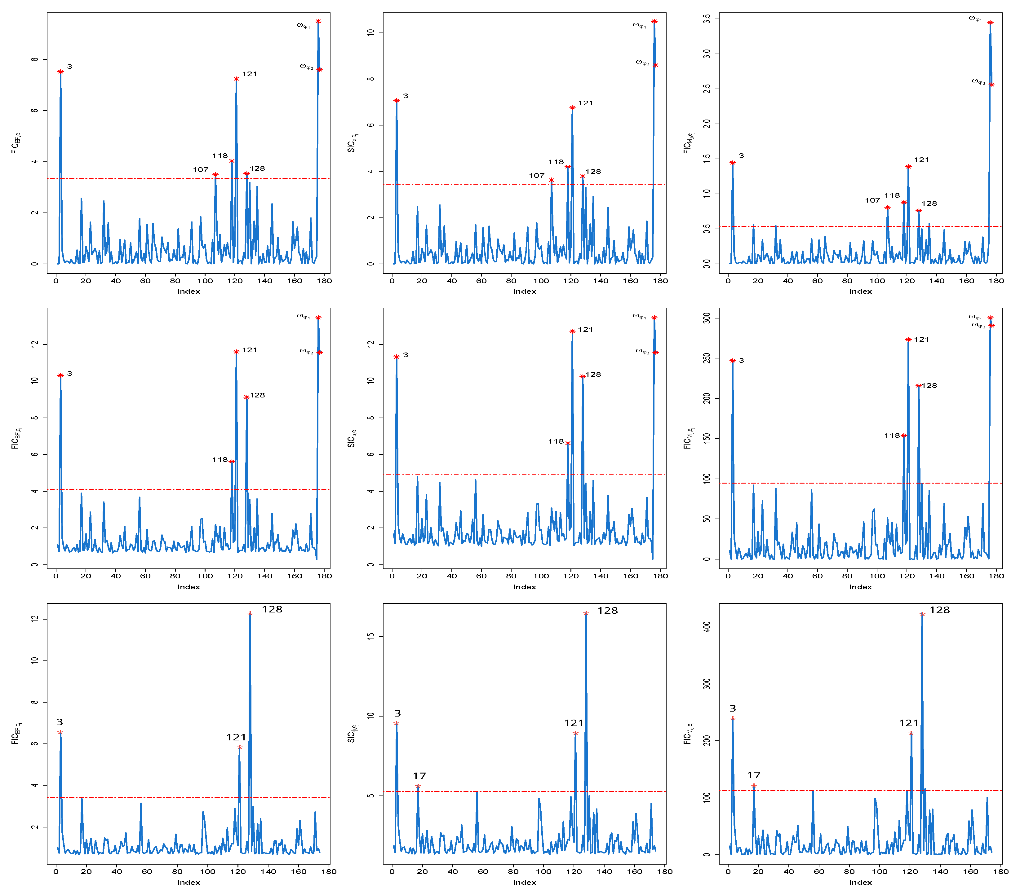
In this real example, the Bayesian local influence diagnostics, which include the Bayes factor (denoted as ${\mathrm{FIC}}_{B,e_j}$), $\varphi$-divergence (represented as ${\mathrm{SIC}}_{\varphi },e_j$), and posterior mean distance (indicated as ${\mathrm{SIC}}_{M_d},e_j$) [21], are assessed based on the parameter vector $d\left(\mathsf{\theta }\right)=(\sqrt{|{\omega }_{\tau 1}|},\dots ,\sqrt{|{\omega }_{\tau 8}|},\sqrt{|{\lambda }_{21}|},\sqrt{|{\lambda }_{31}|},$ $\sqrt{|{\lambda }_{41}|},\sqrt{|{\lambda }_{62}|},\sqrt{|{\lambda }_{72}|},\sqrt{|{\lambda }_{82}|})$. This evaluation is conducted using 200 observations, which were obtained through the previously developed variational Bayesian algorithm in conjunction with the specified prior distributions. In the enchanting field of Bayesian local influence diagnostics, we present our findings alongside their benchmarks, beautifully captured in Figure 1. A closer inspection of this visual wonder reveals that cases 3, 121, and 128 emerge as the stars of the show, wielding their influence across all quantile levels, whether it is $\tau$ = 0.25, 0.5, or 0.75. Meanwhile, case 118 stands out at quantiles $\tau =0.25$ and $0.5$. Case 107, alternatively, is continuously influential at quantile 0.25, irrespective of the local influence metrics used. Notably, the identification of ${\omega }_{\phi }$ as influential by three local influence measures raises concerns about the accuracy of the MAR assumption for missing data.

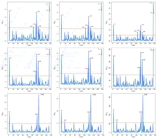
Figure 1. Index plots of Bayesian local influence measures: ${\mathrm{FIC}}_{BF,e_j}$ (left panel), ${\mathrm{SIC}}_{\varphi ,e_j}$ (middle panel) and ${\mathrm{SIC}}_{M_d,e_j}$ (right panel) for $\tau =0.25$ (1st line), 0.5 (2nd line) and 0.75 (3rd line) in a real example.

In order to determine the influence of subjects, case 3, case 118, case 121, and case 128, we recompute the Bayesian estimations for the unknown parameters, omitting these individuals, by applying the variational Bayesian approach introduced earlier along with a mechanism for nonignorable missing data. The Bayesian estimations and their 95% confidence intervals for the parameters in ${\mathsf{\omega }}_{\tau }$, ${\mathsf{\Lambda }}_{\tau }$, ${\mathsf{\Psi }}_{\zeta }$, and $\mathsf{\phi }$, with the exclusion of individuals 128, 121, 118, and 3, are displayed in Table 4. Analysis of Table 4 reveals that the 95% confidence intervals for ${\phi }_1$ and ${\phi }_2$ do not include zero, and the fact that their minimum values are greater than zero substantiates the justification of the nonignorable hypothesis for missing data.

6. Discussion

This investigation considers the complex task of parameter estimation within nonlinear dynamic latent variable models, especially when the challenge of nonignorable missing data is present. These models, marked by their nonlinear latent variables and nonparametric priors, are analyzed using a Bayesian framework. To address the substantial computational demands typically associated with traditional dynamic latent variable models, a novel variational Bayesian technique is introduced to handle missing data and nonlinear dynamics effectively. Utilizing a Dirichlet Process (DP) prior, we can effectively define the unknown distribution of the random effects and integrate it with the variational Bayesian approach. This Bayesian framework has enabled us to develop a practical and robust algorithm that uses an asymmetric Laplace distribution, which combines exponential and normal distributions elegantly. To handle missing data, we employ logistic regression to model the missingness mechanism for observable variables and a truncated normal latent variable with a probit regression model for the propensity scores of missing covariates. In order to handle the mix of continuous and discrete covariates, we conceive a suite of univariate exponential family distributions to portray the joint distribution of the unobserved covariates. We also adapt the Bayesian local influence technique by Zhu et al. [21] to carry out a robustness assessment on quantile nonlinear dynamic latent variable models (DLVMs). Within the variational Bayesian methods framework, we turn the task of precise posterior density estimation into an optimization challenge, focusing on minimizing the evidence lower bound. To ensure computational efficiency, we employ a coordinate ascent algorithm to optimize this lower bound.

Our Bayesian estimates, as evidenced by empirical findings, maintain a high level of accuracy across different quantile levels and missing data mechanisms. We use a real dataset from an EMA study to illustrate our methodologies. However, it is noteworthy that this article refrains from delving into the complexities of high-dimensional random effect models or the more intricate direct relationships between latent variables challenges that are worthy of separate investigation. These engaging issues are perfect for future research pursuits.

References

- Diener, E.; Fujita, F.; Smith, H. The personality structure of affect. J. Personal. Soc. Psychol. 1995, 69, 130–141. [Google Scholar] [CrossRef]
- Chow, S.M.; Nesselroade, J.R.; Shifren, K.; Mcardle, J.J. Dynamic structure of emotions among individuals with parkinson’s disease. Struct. Equ. Model. Multidiscip. J. 2004, 11, 560–582. [Google Scholar] [CrossRef]
- Zhang, Z.Y.; Nesselroade, J.R. Bayesian Estimation of Categorical Dynamic Factor Models. Multivar. Behav. Res. 2007, 42, 729–756. [Google Scholar] [CrossRef]
- Chow, S.M.; Tang, N.S.; Yuan, Y.; Song, X.Y.; Zhu, H.T. Bayesian estimation of semiparametric dynamic latent variable models using the dirichlet process prior. Br. J. Math. Stat. Psychol. 2011, 64, 69–106. [Google Scholar] [CrossRef] [PubMed]
- Tang, N.S.; Chow, S.M.; Ibrahim, J.G.; Zhu, H.T. Bayesian sensitivity analysis of a nonlinear dynamic factor analysis model with nonparametric prior and possible nonignorable missingness. Psychometrika 2017, 82, 875–903. [Google Scholar] [CrossRef] [PubMed]
- Wang, Z.Q.; Tang, N.S. Bayesian quantile regression with mixed discrete and nonignorable missing covariates. Bayesian Anal. 2020, 15, 579–604. [Google Scholar] [CrossRef]
- Tuerde, M.; Tang, N.S. Bayesian semiparametric approach to quantile nonlinear dynamic factor analysis models with mixed ordered and nonignorable missing data. Statistics 2022, 56, 1166–1192. [Google Scholar] [CrossRef]
- Little, R.J.A.; Rubin, D.B. Statistical Analysis with Missing Data, 3rd ed.; John Wiley & Sons: New York, NY, USA, 2019. [Google Scholar]
- Bańbura, M.; Modugno, M. Maximum likelihood estimation of factor models on datasets with arbitrary pattern of missing data. J. Appl. Econ. 2014, 29, 133–160. [Google Scholar] [CrossRef]
- Jungbacker, B.; Koopman, S.J.; van der Wel, M. Maximum likelihood estimation for dynamic factor models with missing data. J. Econ. Dyn. Control 2011, 35, 1358–1368. [Google Scholar] [CrossRef]
- Stock, J.H.; Mark, W.W. Macroeconomic Forecasting Using Diffusion Indexes. J. Bus. Econ. Stat. 2002, 20, 147–295. [Google Scholar] [CrossRef]
- Stock, J.H.; Watson, M.W. Dynamic Factor Models, Factor-Augmented Vector Autoregressions, and Structural Vector Autoregressions in Macroeconomics. In Handbook of Macroeconomics; Elsevier B.V.: Amsterdam, The Netherlands, 2016; pp. 415–525. [Google Scholar]
- Kozumi, H.; Kobayashi, G. Gibbs sampling methods for Bayesian quantile regression. J. Stat. Comput. Simul. 2011, 81, 1565–1578. [Google Scholar] [CrossRef]
- Tang, A.M.; Tang, N.S. Semiparametric Bayesian inference on skew-normal joint modeling of multivariate longitudinal and survival data. Stat. Med. 2015, 34, 824–843. [Google Scholar] [CrossRef] [PubMed]
- Blei, D.; Jordan, M.I. Variational inference for Dirichlet process mixtures. Bayesian Analysis 2006, 1, 121–143. [Google Scholar] [CrossRef]
- Lee, S.Y.; Tang, N.S. Analysis of nonlinear structural equation models with nonignorable missing covariates and ordered categorical data. Stat. Sin. 2006, 16, 1117–1141. [Google Scholar]
- Beal, M.J. Variational Algorithms for Approximate Bayesian Inference. Ph.D. Thesis, University of London, London, UK, 2003. [Google Scholar]
- Bishop, C. Pattern Recognition and Machine Learning; Springer: New York, NY, USA, 2006. [Google Scholar]
- Blei, D.M.; Kucukelbir, A.; McAuliffe, J.D. Variational inference: A review for statisticians. J. Am. Stat. Assoc. 2017, 518, 859–877. [Google Scholar] [CrossRef]
- Durante, D.; Rigon, T. Conditionally Conjugate Mean-Field Variational Bayes for Logistic Models. Stat. Sci. 2019, 34, 472–485. [Google Scholar] [CrossRef]
- Zhu, H.T.; Ibrahim, J.G.; Tang, N.S. Bayesian influence analysis: A geometric approach. Biometrika 2011, 98, 307–323. [Google Scholar] [CrossRef] [PubMed]
Disclaimer/Publisher’s Note: The statements, opinions and data contained in all publications are solely those of the individual author(s) and contributor(s) and not of MDPI and/or the editor(s). MDPI and/or the editor(s) disclaim responsibility for any injury to people or property resulting from any ideas, methods, instructions or products referred to in the content. |
© 2024 by the authors. Licensee MDPI, Basel, Switzerland. This article is an open access article distributed under the terms and conditions of the Creative Commons Attribution (CC BY) license (https://creativecommons.org/licenses/by/4.0/).