Abstract
In this paper, we consider the one-dimensional Ising model (shortly, 1D-MSIM) having mixed spin- with the nearest neighbors and the external magnetic field. We establish the partition function of the model using the transfer matrix. We compute certain thermodynamic quantities for the 1D-MSIM. We find some precise formulas to determine the model’s free energy, entropy, magnetization, and susceptibility. By examining the iterative equations associated with the model, we use the cavity approach to investigate the phase transition problem. We numerically determine the model’s periodicity.
Keywords:
one-dimensional Ising model with mixed spin; free energy; entropy; magnetization; susceptibility; phase transition MSC:
37A25; 37A35; 28D05; 28D20; 37A44
1. Introduction
Lenz introduced the one-dimensional (1D) classical spin-1/2 Ising model [1]. Compared to the spin-1/2 model, the spin-1 Ising model, also known as the Blume–Capel model, is more appropriate; hence, it was employed in the investigation of phase transitions in systems of three states [2,3]. Then, the spin-3/2 Ising model was used to extend the spin-1 Ising model’s conclusions [4,5].
The magnetic characteristics of mixed-spin systems have recently attracted both theoretical and experimental attention [6,7,8]. These systems are especially well suited for studying the magnetic properties of a particular class of magnetic materials, in addition to some technical applications [9]. Therefore, mixed-spin Ising models have been extensively studied in the literature lately [10]. In Ref. [11], we classified the disordered phases corresponding to the Ising model with spin-1 and spin 1/2 on the semi-finite Cayley tree (CT). Then, on the second-order CT, we examined the phase transition problem of the Ising model with spin-2 and spin 1/2. Furthermore, we discussed the chaotic behavior of the corresponding dynamical system [12]. The main methods for examining the properties of Ising models with the mixed spin on the square lattice [10], Bethe lattice [13], and CT [11,12] are Monte Carlo simulations [10], the cavity method [14,15,16], the Kolmogorov consistency method [11,12], the iteration method, and transfer matrix method. In [17], the magneto thermal parameters that characterize the magnetocaloric effect (MCE) behaviors, such as entropy, entropy change, and adiabatic cooling rate, are precisely calculated using the transfer matrix approach.
In the literature, there are numerous methods for determining the free energy of a given model [13,18]. The free energy of the lattice models on the Bethe lattice is calculated while boundary conditions are taken into consideration [13,18,19]. In-depth research has been performed on the thermodynamic properties of the 1D Ising model with single spin-s using the transfer matrix [20,21,22].
The author is not aware of any research on the thermodynamic properties of 1D Ising models with mixed spin. Due to its widespread applications, the matrix transfer approach is one of the most commonly used methods in statistical mechanics. In [21], the transfer matrix approach is considered to conduct an analytical study of the 1D Ising model with spin-s. To grasp physical issues as well as statistical mechanics, it is essential to compute thermodynamic quantities like free energy, entropy, magnetization, and magnetic susceptibility [22].
In this paper, to determine the thermodynamic quantities related to 1D-MSIM with the mixed spin-, we consider the transfer matrix approach. We enlarge a specific bond and establish the transfer matrix that corresponds to the bond from site j to site . By considering the trace of several transfer matrices multiplied simultaneously, the partition function is reconstructed. Inspired by the results given for the 1D Ising model with the single spin-s [21], the partition function and the free energy of 1D-MSIM with mixed spin- having the nearest neighbor interactions and external field are calculated. To calculate the model’s free energy, entropy, magnetization, and susceptibility, some exact formulas are established via the corresponding transfer matrix. By using the cavity approach to the corresponding iterative equations of the model, the phase transition issue is studied. The periodicity of the model is also estimated, numerically.
2. Preliminaries
Here, we review definitions and key findings in the construction of the partition function for the 1D-MSIM with mixed spin- on the one-dimensional lattice . We denote the set of integers by and the set of strictly positive integers by . Two vertices x and y, are called nearest-neighbor (NN) if there exists an edge connecting them, which is denoted by . For , the distance is the length (the number of edges) of the shortest path connecting x with y. For any , the direct successor of the vertex x is defined by
Denote the set of even natural numbers by and the set of odd natural numbers by . We consider the mixed spin-state spaces denoted by and . For , a spin configuration on A is defined as a function.
Let us consider finite set . Let and be the spaces of infinite configurations and and be the spaces of finite configurations. represents the configuration space. An element of is denoted by , for . Similarly, an element of is denoted by , for
In this paper, the spins in and can be placed on the odd-numbered vertices and the even-numbered vertices, respectively, when mixed spins are designed on the lattice (see Figure 1).
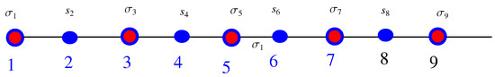
Figure 1.
Configurations with a mixed spin on a one-dimensional finite block, where and for
Construction of the Partition Function Associated with the Model
Let us construct the partition function corresponding to 1D-MSIM with mixed spin on the lattice .
Let , so that one has
where and .
Fix a finite volume . Let be the set of nearest-neighbor edges with at least one endpoint in . We examine in detail the 1D-MSIM with mixed spin built on the lattice , having the Hamiltonian
where the energy of each link tying up nearby sites is represented by the first sum, and the energy of each site is represented by the second sum.
The partial partition functions associated with the Hamiltonian (1) can be found as follows:
where , and J is the coupling constant.
Given the finite set , by considering the boundary spins, or the spins on the -th level, we can construct the summation of Equation (2). Consequently, we state that the density-free energy function is
where is the total partition function.
As a result of the derivatives of the free energy function with respect to certain parameters, many authors have studied other thermodynamic properties [21,22]. If the largest eigenvalue of the transfer matrix corresponding to the given model is , the thermodynamic quantities of this system are obtained as follows:
- Bulk free energy
- Entropy
- Internal energy
3. Construction of the Partition Function for the Model via Transfer Matrices
The Kramers–Wannier transfer technique may be used to construct the partition function. This method requires building a transfer matrix and determining its eigenvalues.
3.1. The Partition Function and the Boltzmann Weight
It is well known that the total partition function depends on the particular realization (see [21,22] for details). Also, it is well known that the total partition function is equal to the Boltzmann weight’s sum over all possible states. Here, we consider blocks or configurations with length, and under zero boundary conditions, that is, the spins designed for are regarded as .
If we want to rewrite the Hamiltonian (1) for all configurations on the configuration space , we can obtain the Boltzmann weight in the form:
From (1), for , we denote the energy of the bond between sequential vertices and by
Similarly, for we denote the energy of the bond between sequential vertices and by
Note that, as can be seen in Equations (8) and (9), for , while the oscillating magnetic fields and fluctuate depending on where the vertex is located, the coupling constant J, which determines the energy between two successive vertices, remains constant.
It is well known that the partition function is equal to the sum of the Boltzmann weight over all possible states in the lattice [21,22]. Therefore, for the configuration , we can write the Boltzmann weight in the form
For this system, the canonical partition function can be written as
The next step is to decompose the bonds using the bond representation and factor the Boltzmann weights into pairwise factors.
3.2. The Transfer Matrices
Here, we construct the transfer matrices corresponding to 1D-MSIM with the mixed spin on the lattice . We obtain two different transfer matrices. First, let us place the spins of the set on the odd-numbered vertices of the lattice , and the spins in the set on the even-numbered vertices. So, we define the entries of the transfer matrix as follows:
where and for .
Similarly, we can define the entries of the transfer matrix by
where and for .
3.3. 1D-MSIM with Mixed Spin-
Due to the difficulty of computation of the transfer matrix and its eigenvalues for and , we restrict ourselves to the mixed spin . In this subsection, we compute the thermodynamic quantities of 1D-MSIM with mixed spin . So, we consider the mixed spins as and .
Firstly, let us construct the transfer matrix as , for and . So, we have
Secondly, let us place the spins of the set on the even-numbered vertices of the lattice , and the spins in the set on the odd-numbered vertices (see Figure 1). We can define the second transfer matrix , for and as
3.4. Investigation of Thermodynamic Quantities in the Translation-Invariant Case
Assume that for all and . This case is called the translation-invariant property. Thus, the transfer matrices and given in (15) and (16) are obtained as follows
Case I
When we multiply the transfer matrices and given in Equations (17) and (18), we obtain the square matrix:
After some tedious and complicated algebraic manipulations, the eigenvalues of the matrix are obtained as:
where
For the sake of simplicity, substitute the variables and to obtain
By computing the trace of the matrix product , we can determine the partition function as
where denotes the eigenvalues of the transfer matrix for
From (11), we obtain
where denote the eigenvalues of transfer matrix .
So, one has for . As it is well known, the model’s critical behavior manifests itself in the thermodynamic limit as ; therefore, the largest eigenvalue of the transfer matrix given in (19) stands as the only indicator of the bulk free energy:
3.5. Behavior of the Thermodynamic Quantities of 1D-MSIM with Mixed Spin-(s,(2t − 1)/2) in the Absence of a Magnetic Field
For , we obtain the transfer matrix given in (19) as
The set of eigenvalues of the matrix is obtained as follows:
It is clear that From the formula in (23), we obtain
Figure 2 shows the graph of free energy given in (25) as a function of for . From Figure 2, it can be seen that the free energy is approaching zero for . In Figure 2, the oscillating magnetic fields and are assumed to be zero. If and are taken to be nonzero, then, by using the parametric representation, the free energy function can be plotted in the form .
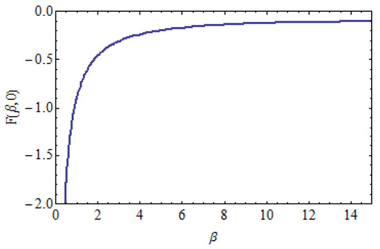
Figure 2.
The graph of free energy given in (25) as a function of for .
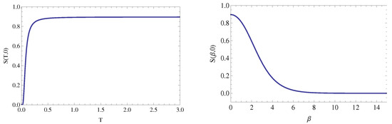
In the absence of an external magnetic field, from (5), the entropy of the model is obtained as
Similarly, from (6), we obtain the internal energy as
The changes in entropy of 1D-MSIM with mixed spin are given in Figure 3. Results show that the internal energy converges to zero at the higher temperature values, while becoming a constant 0 as . When the temperature increases, the entropy increases until it reaches and goes to zero at low temperature values.
Case II
Note that while successively placing spins on the vertices of a one-dimensional lattice, if the elements of are placed in the first vertex of the lattice , then a transfer matrix having dimensions is obtained, and the eigenvalues of the transfer matrix are the same as those of the previous matrix .
If we substitute the variables and for simplicity, we obtain
We obtain the set of eigenvalues of the matrix given in as
It should be noted here that the eigenvalues of the matrices and are the same, except for 0. Therefore, it is obtained that (see Equations (20) and (30)). We can choose any spin on the starting vertex, while mixed spins are placed on consecutive vertices of the lattice. From (20) and (30), it is clear that .
3.6. Magnetization and Magnetic Susceptibility
In this subsection, we construct magnetization and magnetic susceptibility by means of the eigenvalue in the Formula (30).
Let us consider the reduced nearest neighbor spin–spin coupling interactions and the reduced magnetic field , we write the magnetization as
and susceptibility
We do not give the exact expressions of the formulas for the magnetization and susceptibility here, because the operations are excessively long and complex. We numerically examine the behavior of these two quantities as functions of h and T.
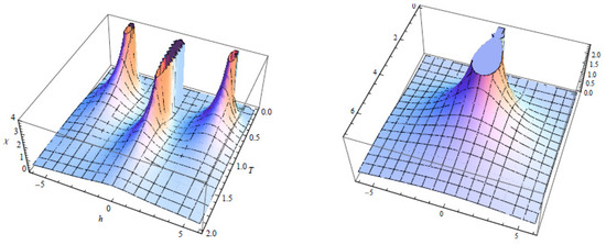
The Mathematica software (Version 8.0, Wolfram Research, Inc., Champaign, IL, USA) [23] has been used to perform the calculations and to plot the figures. A three-dimensional plot of is given in Figure 4. Taking into account the eigenvalue in the Formula (30), for , one can easily see that, as the temperature T increases, the smoothness of the function decreases and exhibits a behavior similar to the step function. On the other hand, for , the surface of the function becomes smooth. In contrast to the single-spin Ising chain’s typical single step [21], in Figure 4 (left), the magnetization graph shows three distinct steps at low temperatures. This phenomenon may be explained by spins adopting distinct states within even and odd sublattices, or by all spins assuming the same state.
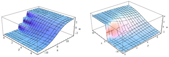
A three-dimensional plot of is given in Figure 5. Figure 5 (Left) and (Right) show the behavior of the susceptibility function given in Equation (32). For , three stacks resembling a boot are observed, and a stack appears for in the chosen region , . As seen in Figure 5 (Left), while three different susceptibility peaks appear for at low temperatures, the susceptibility peaks disappear as the temperature increases. For , only a single susceptibility peak is observed at low temperatures (see Figure 5 (Right)).
4. Nonexistence Phase Transition in the Absence of the External Magnetic Field
In this section, we study 1D-MSIM with the mixed spin-(1,1/2) employing the ERR.
If we assume , and , then we obtain a new three-dimensional rational dynamical system (3D-RDS) as
If the values of x and y in Equations (37) and (38) are substituted into Equation (36), one obtains the following rational recursive equation :
From (39), we obtain a second-order equation
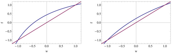
From Equation (40), it is clear that the function f given in (39) has only one positive fixed point, so there is no phase transition for the given model.
The graphs of the function f for antiferromagnetic () and ferromagnetic () values are plotted in Figure 6. The diagrams show that the function in both cases has just two fixed points. Additionally, there is only one positive fixed point. As a result, there is just one Gibbs measure and no phase transition in the model. As it is well known, the classical single spin 1D Ising model’s phase transition issue has attracted the interest of statistical mechanics researchers for over a century, and it has been established that there is no phase transition [1]. In this present paper, we demonstrated that the mixed spin 1D Ising model has no phase transition as an example.
Chaoticity of the Model
A dynamical system’s chaotic behavior is determined by how sensitively it depends on the initial conditions [24,25]. It has long been a challenge to see whether a model’s phase transition and the chaotic behavior of the corresponding dynamical system are related [26]. In this subsection, we investigate the chaoticity of the 3D-RDS given in (36)–(38). With the help of the Lyapunov exponent, we numerically study the model’s chaotic behavior.
Figure 7 shows the Lyapunov exponent of the dynamical system corresponding to the 1D-MSIM with mixed spin-(1,1/2). It is seen that the Lyapunov exponent is always negative in the ferromagnetic region. Therefore, the rational function given in (39) is periodic. The behavior of the Lyapunov exponent in the antiferromagnetic region can also be examined.
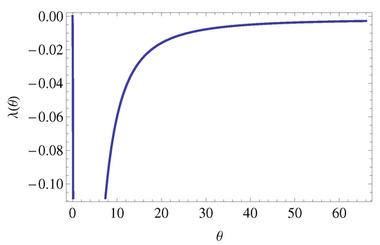
Figure 7.
The graph of the function given in (42) versus in the ferromagnetic region ().
5. The Average Magnetization for the Mixed Spin-(1,1/2) Ising Model
In this section, by using the exact recursion relations (ERRs) (see [9]), we obtain the partial partition functions of the 1D-MSIM with mixed spin-. Contrary to the previous sections, here we place the spins of in the first vertex of the lattice and the spins of in the second vertex of the lattice, while placing spins at the vertices of the lattice , so for , we obtain and . With the help of the cavity method (see [14,15,16] for details), we obtain the partial partition functions as follows:
The Average Magnetization
In this subsection, assuming there is an external magnetic field, we obtain the magnetization equations for spins s and , respectively, as follows.
6. Conclusions
There are many methods for calculating the free energy of lattice models on the Bethe lattices or the d-dimensional integer lattice (). Some of these are the exact recursion relations [9], the cavity method [18], and vector-valued boundary conditions. One of the most widely used methods to examine thermodynamic quantities corresponding to a 1D Ising model is the transfer matrix technique [21,22]. In this present work, we constructed the partial partition functions associated with 1D-MSIM having mixed spin- via the transfer matrix. We have computed some thermodynamic quantities such as the free energy, entropy, magnetization, and susceptibility of the model. To the best of my knowledge, the thermodynamic properties of the 1D Ising model with the single spin have been investigated in several studies to date. Using the transfer matrix method, we evaluated the thermodynamic features of the 1D-MSIM for the first time. For the single spin-Isign model, Amin et al. [21] plotted the magnetization and susceptibility in two dimensions.
In our previous studies, we proved that there is a phase transition for the mixed-spin Ising model on the CT using many methods [11,12,14]. As it is known, there is no phase transition for a single spin 1D Ising model [1]. In this study, we investigated how mixed spins affect thermodynamic quantities and the existence of the phase transition. We demonstrated the uniqueness of limiting Gibbs measures associated with 1D-MSIM having mixed spin-(1,1/2). We have shown that if the external magnetic field is zero, for the aforementioned model, there is no phase transition. Our next research will deal with other issues in statistical mechanics. By considering the approach given by Albayrak [9], the isothermal entropy change of the average magnetization for 1D-MSIM will be analyzed.
The findings obtained in our present article exhibit different behaviors from the results given in previous studies [21,22]. Frankly, we cannot comment on the physical meaning of such behavior. These topics are covered in introductory courses in statistical mechanics at the undergraduate level. Therefore, we believe that the results of our present study will be of interest to a wide readership of statistical mechanics.
Funding
This research received no external funding.
Data Availability Statement
The statistical data presented in the article do not require copyright. They are freely available and are listed at the reference address in the bibliography.
Acknowledgments
The author would like to thank the Simons Foundation (10.13039/100000893) and the Institute of International Education for their support. While the author was a visiting scientist at the ICTP, a significant part of the research was completed there. The author therefore thanks ICTP for their hospitality. The author expresses gratitude to the referees for their comments and suggestions.
Conflicts of Interest
The author declare no conflict of interest.
References
- Ising, E. Beitrag zur theorie des ferromagnetismus. Z. Physik 1925, 31, 253. [Google Scholar] [CrossRef]
- Blume, M. Theory of the first-order magnetic phase change in UO2. Phys. Rev. 1966, 141, 517. [Google Scholar] [CrossRef]
- Capel, H.W. On the possibility of first-order phase transitions in Ising systems of triplet ions with zero-field splitting. Physica 1966, 32, 966. [Google Scholar] [CrossRef]
- Lipowski, A.; Suzuki, M. On the exact solution of twodimensional spin S Ising models A. Phys. A 1993, 193, 141. [Google Scholar] [CrossRef]
- Izmailian, N.S.; Ananikian, N.S. General spin-3/2 Ising model in a honeycomb lattice: Exactly solvable case. Phys. Rev. B 1994, 50, 6829. [Google Scholar] [CrossRef]
- De La Espriella, N.; Arenas, A.J.; Paez Meza, M.S. Critical and compensation points of a mixed spin-2-spin-5/2 Ising ferrimagnetic system with crystal field and nearest and next-nearest neighbors interactions. J. Magn. Magn. Mater. 2016, 417, 434–441. [Google Scholar] [CrossRef]
- De La Espriella, N.; Buendia, G.M.; Madera, J.C. Mixed spin-1 and spin-2 Ising model: Study of the ground states. J. Phys. Commun. 2018, 2, 025006. [Google Scholar] [CrossRef]
- Kaneyoshi, T. Phase transition of the mixed spin system with a random crystal field. Phys. A 1988, 153, 556–566. [Google Scholar] [CrossRef]
- Albayrak, E. The study of mixed spin-1 and spin-1/2: Entropy and isothermal entropy change. Phys. A 2020, 559, 125079. [Google Scholar] [CrossRef]
- De La Espriella, N.; Buendia, G.M. Magnetic behavior of a mixed Ising 3/2 and 5/2 spin model. J. Phys. Condens. Matter 2011, 23, 176003. [Google Scholar] [CrossRef]
- Akın, H.; Mukhamedov, F. Phase transition for the Ising model with mixed spins on a Cayley tree. J. Stat. Mech. 2022, 2022, 053204. [Google Scholar] [CrossRef]
- Akın, H. The classification of disordered phases of mixed spin (2,1/2) Ising model and the chaoticity of the corresponding dynamical system. Chaos Solitons Fractals 2023, 167, 113086. [Google Scholar] [CrossRef]
- Seino, M. The free energy of the random Ising model on the Bethe lattice. Phys. A 1992, 181, 233–242. [Google Scholar] [CrossRef]
- Akın, H. Quantitative behavior of (1,1/2)-MSIM on a Cayley tree. Chin. J. Phys. 2023, 83, 501–514. [Google Scholar] [CrossRef]
- Ostilli, M. Cayley Trees and Bethe Lattices: A concise analysis for mathematicians and physicists. Phys. A 2012, 391, 3417–3423. [Google Scholar] [CrossRef]
- Mézard, M.; Parisi, G. The Bethe lattice spin glass revisited. Eur. Phys. J. B 2001, 20, 217–233. [Google Scholar] [CrossRef]
- Qi, Y.; Liu, J.; Yu, N.-S.; Du, A. Magnetocaloric effect in ferroelectric Ising chain magnet. Solid State Commun. 2016, 233, 1–5. [Google Scholar] [CrossRef]
- Akın, H. Calculation of the free energy of the Ising model on a Cayley tree via the self-similarity method. Axioms 2022, 11, 703. [Google Scholar] [CrossRef]
- Akın, H.; Ulusoy, S. A new approach to studying the thermodynamic properties of the q-state Potts model on a Cayley tree. Chaos Solitons Fractals 2023, 174, 113811. [Google Scholar] [CrossRef]
- Salinas, S.R.A. Phase Transitions and Critical Phenomena: Classical Theories. In Introduction to Statistical Physics. Graduate Texts in Contemporary Physics; Springer: New York, NY, USA, 2001. [Google Scholar]
- Amin, M.E.; Mubark, M.; Amin, Y. On the critical behavior of the spin-s ising model. Rev. Mex. Fis. 2023, 69, 021701. [Google Scholar] [CrossRef]
- Wang, W.; Diaz-Mendez, R.; Capdevila, R. Solving the one-dimensional Ising chain via mathematical induction: An intuitive approach to the transfer matrix. Eur. J. Phys. 2019, 40, 065102. [Google Scholar] [CrossRef]
- Mathematica, Version 8.0; Wolfram Research, Inc.: Champaign, IL, USA, 2010.
- Feigenbaum, M.J. Quantitative universality for a class of nonlinear transformations. J. Stat. Phys. 1978, 19, 25–52. [Google Scholar] [CrossRef]
- Feigenbaum, M.J. Universal behavior in nonlinear systems. Phys. D 1983, 7, 16–39. [Google Scholar] [CrossRef]
- Hilborn, R.C. Chaos and Nonlinear Dynamics: An Introduction for Scientists and Engineers; Oxford University Press on Demand: Oxford, UK, 2000. [Google Scholar]
Disclaimer/Publisher’s Note: The statements, opinions and data contained in all publications are solely those of the individual author(s) and contributor(s) and not of MDPI and/or the editor(s). MDPI and/or the editor(s) disclaim responsibility for any injury to people or property resulting from any ideas, methods, instructions or products referred to in the content. |
© 2023 by the author. Licensee MDPI, Basel, Switzerland. This article is an open access article distributed under the terms and conditions of the Creative Commons Attribution (CC BY) license (https://creativecommons.org/licenses/by/4.0/).