A Perturbed Milne’s Quadrature Rule for n-Times Differentiable Functions with L^p-Error Estimates

Abstract

In this work, a perturbed Milne’s quadrature rule for n-times differentiable functions with $L^p$-error estimates is derived. One of the most important advantages of our result is that it is verified for p-variation and Lipschitz functions. Several error estimates involving $L^p$-bounds are proven. These estimates are useful if the fourth derivative is unbounded in $L^{\infty }$-norm or the $L^p$-error estimate is less than the $L^{\infty }$-error estimate. Furthermore, since the classical Milne’s quadrature rule cannot be applied either when the fourth derivative is unbounded or does not exist, the proposed quadrature could be used alternatively. Numerical experiments showing that our proposed quadrature rule is better than the classical Milne rule for certain types of functions are also provided. The numerical experiments compare the accuracy of the proposed quadrature rule to the classical Milne rule when approximating different types of functions. The results show that, for certain types of functions, the proposed quadrature rule is more accurate than the classical Milne rule.

1. Introduction

There are many attractive methods that are used to approximate real integrals. One of the oldest and most well known is the Newton–Cotes closed and open formulas. Particularly, among other famous formulas; Simpson’s rule and Milen’s rule are very interesting and close to each other. Each formula involves a bounded error of the fourth degree. However, it is well known that Simpson’s rule is of closed Newton-type formula, while Milne’s formula is of open type. Accordingly, it is very interesting to test both quadrature rules in many situations. In recent decades, the modern theory of inequalities are used at large to verify these quadrature rules (and others) using the Peano-kernel approach.

In terms of Newton–Cotes formulas, Milne’s open-type formula is parallel to Simpson’s closed-type formula, since they are held under the same conditions. Suppose $g\in C^4\left([c,d]\right)$, and

$$\begin{array}{c}\hfill {∥g^{\left(4\right)}∥}_{\infty }:=\underset{s\in \left(c,d\right)}{sup}\left|g^{\left(4\right)}\left(s\right)\right|<\infty .\end{array}$$

In terms of inequalities Simpson and Milne’s inequalities are read, respectively, [1]:

$$\begin{array}{c}\hfill \left|\frac{d-c}{3}\left[\frac{g\left(c\right)+g\left(d\right)}{2}+2g\left(\frac{c+d}{2}\right)\right]-{\int }_c^{d}g\left(s\right)ds\right|\le \frac{{\left(d-c\right)}^5}{2880}{∥g^{\left(4\right)}∥}_{\infty },\end{array}$$

(1)

and

$$\begin{array}{c}\hfill \left|\frac{d-c}{3}\left[2g\left(\frac{3c+d}{4}\right)-g\left(\frac{c+d}{2}\right)+2g\left(\frac{c+3d}{4}\right)\right]-{\int }_c^{d}g\left(s\right)ds\right|\le \frac{7{\left(d-c\right)}^5}{23040}{∥g^{\left(4\right)}∥}_{\infty }.\end{array}$$

(2)

Our study indicates that attempting to apply Simpson and Milne’s quadrature rules using lower-order derivations can prove highly promising (especially for certain types of functions). In the past few years, Simpson’s formula has already taken a serious place in many published works, see, for example, [2,3,4,5,6,7,8,9,10,11,12,13]. On the other hand, Milne’s rule is less popular than Simpson’s for a number of reasons. Milne’s quadrature rule, however, has not attracted many experimenters. This is because Milne’s rule is more difficult to implement and can be more prone to numerical errors. Additionally, Simpson’s rule tends to be more accurate and efficient, meaning that Milne’s rule is often not seen as the best option.

Because of this, we concentrate this work on studying the error of Milne’s quadrature rule for n-times differentiable functions by carrying several $L^p$ bounds of this quadrature.

Furthermore, the considered approach allows us to see how adding derivations of the bumps of this rule oscillate its error term. In other words, how Milne’s quadrature rule behaves as a predictor for advanced or lower derivations. In fact, the oscillation of the proposed quadrature rule rises in general. This indicates that Milne’s quadrature rule is more accurate for higher-order derivations, making it a better predictor of more complicated functions. This is because the rule is able to more accurately capture the behaviour of the underlying function.

On the other hand, it is shown numerically and virtually that, for certain types of functions, the error descends rapidly, meaning our approach could be practical for certain types of functions. Furthermore, one of the most significant advantages of our result is that it is validated for p-variation and Lipschitz functions. Moreover, since the classical Milne’s quadrature rule (2) cannot be applied when the fourth derivative is unbounded or absent, the proposed quadrature could be used alternately. This could significantly expand our understanding of Milne’s quadrature rule and its applications. It could also provide new insights into the mathematical analysis of problems involving unbounded or absent fourth derivatives. This could ultimately lead to the development of more efficient numerical algorithms for solving such problems.

Quadrature rules involving $L^p$ norms are less popular than existing ones involving $L^{\infty }$ norms. This is because the $L^p$ norms are more difficult to work with due to their non-uniformity. Furthermore, it is not straightforward to construct quadrature rules that are exact for high-degree polynomials in these cases. As a result, it is often preferable to use the $L^{\infty }$ norm. However, the $L^p$ norms are more effective when dealing with functions that are not smooth. This is because the $L^p$ norms are more sensitive to small changes in the function, which allows for more accurate approximations of non-smooth functions. Moreover, the $L^p$ norms can be used to construct quadrature rules that are exact for polynomials of any degree, whereas the $L^{\infty }$ norm is limited to low-degree polynomials. As such, they can be a useful method for approximating certain classes of functions. For example, the $L^2$ norm is especially useful for approximating functions with discontinuities. In addition, it can be more efficient than the $L^{\infty }$ norm in cases where the function is not well-behaved. The $L^p$ norms can also be used to approximate functions that are not continuous, such as functions with sharp edges. In such cases, the $L^p$ norm can provide a more accurate approximation than the $L^{\infty }$ norm. The $L^1$ norm can also be used to approximate discontinuous functions, but it tends to be less accurate than the $L^2$ and $L^p$ norms. This is because the $L^2$ norm looks at the average of the values of the function over a region and the $L^{\infty }$ norm looks at the maximum value of the function over a region. This means that the $L^p$ norm can capture local features in the function that the $L^{\infty }$ norm cannot. Additionally, the $L^1$ norm is more sensitive to outliers than the $L^2$ and $L^p$ norms, leading to inaccurate approximations in certain cases.

For more about similar quadrature rules and other related results, the reader is referred to [14,15,16,17,18,19,20,21,22,23,24,25,26,27,28,29,30,31,32,33,34,35,36,37]. For other closely related results using another approach see [38,39,40,41,42,43,44,45,46,47,48] and the references therein. For classical methods of integral approximations see [32,49]. The book [50], is also recommended for recent and classical methods of numerical integration.

In light of the foregoing, Milne’s recommendation of using the three-point Newton–Cotes open formula as a predictor rule and the three-point Newton–Cotes closed formula (Simpson’s rule) as a corrector rule for fourth differentiable functions with bounded derivatives. In this work, a perturbed Milne’s quadrature rule for n-times differentiable functions with $L^p$-error estimates is derived.

One of the most important advantages of our result is that it is verified for p-variation and Lipschitz functions. Several error estimates involving $L^p$-bounds are proven. These estimates are useful if the fourth derivative is unbounded in $L^{\infty }$-norm or the $L^p$-error estimate is less than the $L^{\infty }$-error estimate. Furthermore, since the classical Milne’s quadrature rule cannot be applied either when the fourth derivative is unbounded or does not exist, the proposed quadrature could be used alternatively. By extending these formulas to other $L^p$ spaces, we can increase the accuracy of the numerical analysis even further. Often, we need to approximate real integrals under the assumptions of the function involved. Because of this, this work is focused on introducing several $L^p$ error estimates for the proposed perturbed Milne’s quadrature rule. Furthermore, we can obtain better approximate integrals that involve functions with more complex structures, and a better understanding of how the function behaves in different spaces with more accurate predictions about the integral’s value.

Additionally, by accounting for the structure of the function, we can create more accurate estimates for the error of the quadrature rule. For instance, the error of the quadrature rule when calculating an integral in an $L^2$ space is typically smaller than when calculating an integral in an $L^1$ space, due to the $L^2$ space being better suited to represent the structure of the function being integrated. Furthermore, the structure of the function influences the integration accuracy. For example, functions with higher-order derivatives require more accurate quadrature rules in order to achieve the same level of accuracy. Additionally, the function’s smoothness also plays a role in the integration accuracy. This provides a more precise approximation of the integral, leading to more accurate numerical analysis. Numerical experiments showing that our proposed quadrature rule is better than the classical Milne’s rule for certain types of functions are also provided. Moreover, the demonstration of the examples reflects the effectiveness of the proposed quadrature rule for certain types of functions. The numerical experiments compare the accuracy of the proposed quadrature rule to the classical Milne’s rule when approximating different types of functions. The results show that, for certain types of functions, the proposed quadrature rule is more accurate than the classical Milne’s rule. This suggests that the proposed quadrature rule could be an effective tool for approximating integrals with high accuracy, and the results could also be used to inform future research on perturbed quadrature rules.

2. Perturbed Milne’s Quadrature Formula

In order to establish our results we need to recall the following two lemmas.

Lemma 1

([16]). Fix $1\le p<\infty$. Assume that g is a continuous function on $[c,d]$ and w is of bounded p–variation on $[c,d]$. Then ${\int }_c^{d}g\left(s\right)dw\left(s\right)$, exists and the inequality:

$$\begin{array}{c}\hfill \left|{\int }_c^{d}g\left(s\right)dw\left(s\right)\right|\le {∥g∥}_{\infty }·\underset{c}{\overset{d}{\bigvee }}\left(w;p\right),\end{array}$$

(3)

holds, where ${\displaystyle \underset{c}{\overset{d}{\bigvee }}}\left(w,p\right)$ denotes the total p-variation of w over $[c,d]$.

Lemma 2

([16]). Let $1\le p<\infty$. Assume that $g\in L^p[c,d]$ and w has a Lipschitz property on $[c,d]$. Then

$$\begin{array}{c}\hfill \left|{\int }_c^{d}g\left(s\right)dw\left(s\right)\right|\le Li{p}_M\left(w\right){(d-c)}^{1-\frac{1}{p}}·{∥g∥}_p,\end{array}$$

(4)

holds.

From now on I is a real interval and $c,d\in \mathbb{R}$ with $c,d\in I^{\circ }$ is the interior of I with $c<d$. The set ${\mathfrak{V}}_p^{\left(m\right)}$ is defined to be the set of all m-times continuously differentiable functions g whose m-derivative $(m\ge 1)$ is absolutely continuous with $g^{\left(m\right)}\in L^p[c,d]$$(1\le p\le \infty )$.

In what follows, we present a primary result involving the expansion of Milne’s rule for higher-order derivatives using the Peano-kernel approach.

Lemma 3.

If $g\in {\mathfrak{V}}_1^{\left(m\right)}$, then we have

$$\begin{array}{cc}\hfill & {\int }_c^{d}g\left(s\right)ds\hfill \\ \hfill & =\sum _{\ell =0}^{m-1}\frac{{\left(d-c\right)}^{\ell +1}}{\left(\ell +1\right)!}\left\{\left[{\left(\frac{5}{12}\right)}^{\ell +1}+{\left(\frac{1}{4}\right)}^{\ell +1}\right]\left[g^{(\ell )}\left(\frac{3c+d}{4}\right)+{\left(-1\right)}^{\ell }{g}^{(\ell )}\left(\frac{c+3d}{4}\right)\right]\right.\hfill \\ \hfill & \left.-\frac{\left({\left(-1\right)}^{\ell }+1\right)}{6^{\ell +1}}{g}^{(\ell )}\left(\frac{c+d}{2}\right)\right\}+{\left(-1\right)}^m{\int }_c^d{\mathcal{K}}_m\left(s\right)g^{\left(m\right)}\left(s\right)ds,\hfill \end{array}$$

(5)

where

$$\begin{array}{c}\hfill {\mathcal{K}}_m\left(s\right)=\left\{\begin{array}{c}\frac{1}{m!}{\left(s-c\right)}^m,\mathrm{if}s\in \left[c,\frac{3c+d}{4}\right]\hfill \\ \\ \frac{1}{m!}{\left(s-\frac{c+2d}{3}\right)}^m,\mathrm{if}s\in \left(\frac{3c+d}{4},\frac{c+d}{2}\right]\hfill \\ \\ \frac{1}{m!}{\left(s-\frac{2c+d}{3}\right)}^m,\mathrm{if}s\in \left(\frac{c+d}{2},\frac{c+3d}{4}\right]\hfill \\ \\ \frac{1}{m!}{\left(s-d\right)}^m,\mathrm{if}s\in \left(\frac{c+3d}{4},d\right]\hfill \end{array}\right.\end{array}$$

for all $m\ge 1$.

Proof. 

We carry out our proof using mathematical induction. For $m=1$ we have

$$\begin{array}{c}\hfill {\mathcal{K}}_1\left(t\right)=\left\{\begin{array}{c}s-c,s\in \left[c,\frac{3c+d}{4}\right]\hfill \\ \\ s-\frac{c+2d}{3},s\in \left(\frac{3c+d}{4},\frac{c+d}{2}\right]\hfill \\ \\ s-\frac{2c+d}{3},s\in \left(\frac{c+d}{2},\frac{c+3d}{4}\right]\hfill \\ \\ s-d,s\in \left(\frac{c+3d}{4},d\right]\hfill \end{array}\right..\end{array}$$

By applying the integration by parts, we obtain

$$\begin{array}{c}\hfill {\int }_c^{\frac{3c+d}{4}}{\mathcal{K}}_1\left(s\right)dg\left(s\right)=\left(\frac{d-c}{4}\right)g\left(\frac{3c+d}{4}\right)-{\int }_c^{\frac{3c+d}{4}}g\left(s\right)ds,\end{array}$$

$$\begin{array}{c}{\int }_{\frac{3c+d}{4}}^{\frac{c+d}{2}}{\mathcal{K}}_1\left(t\right)dg\left(s\right)\hfill \\ \hfill =\left(\frac{c+d}{2}-\frac{c+2d}{3}\right)g\left(\frac{c+d}{2}\right)-\left(\frac{3c+d}{4}-\frac{c+2d}{3}\right)g\left(\frac{3c+d}{4}\right)-{\int }_{\frac{3a+b}{4}}^{\frac{c+d}{2}}g\left(s\right)ds,\end{array}$$

$$\begin{array}{c}{\int }_{\frac{c+d}{2}}^{\frac{c+3d}{4}}{\mathcal{K}}_1\left(t\right)dg\left(s\right)=\hfill \\ \hfill \left(\frac{c+3d}{4}-\frac{2c+d}{3}\right)g\left(\frac{c+3d}{4}\right)-\left(\frac{c+d}{2}-\frac{2c+d}{3}\right)g\left(\frac{a+b}{2}\right)-{\int }_{\frac{c+d}{2}}^{\frac{c+3d}{4}}g\left(s\right)ds,\end{array}$$

and

$$\begin{array}{c}\hfill {\int }_{\frac{c+3d}{4}}^b{\mathcal{K}}_1\left(s\right)dg\left(s\right)=\left(\frac{d-c}{4}\right)g\left(\frac{c+3d}{4}\right)-{\int }_{\frac{c+3d}{4}}^{b}g\left(s\right)ds.\end{array}$$

By adding the above equalities and arranging the resulting terms, simple calculations yield that

$$\begin{array}{c}\hfill {\int }_c^{d}g\left(s\right)ds=\frac{\left(d-c\right)}{3}\left[2g\left(\frac{3c+d}{4}\right)-g\left(\frac{c+d}{2}\right)+2g\left(\frac{c+3d}{4}\right)\right]-{\int }_c^d{\mathcal{K}}_1\left(s\right)dg\left(s\right).\end{array}$$

Now, we assume that (5) holds for $m=l$. We need to show that it holds for $m=l+1$, i.e.,

$$\begin{array}{cc}\hfill & {\int }_c^{d}g\left(s\right)ds\hfill \\ \hfill & =\frac{\left(d-c\right)}{3}\left[2g\left(\frac{3c+d}{4}\right)-g\left(\frac{c+d}{2}\right)+2g\left(\frac{c+3d}{4}\right)\right]\hfill \\ \hfill & +\sum _{\ell =1}^l\frac{{\left(d-c\right)}^{\ell +1}}{\left(\ell +1\right)!}\left\{\left[{\left(\frac{5}{12}\right)}^{\ell +1}+{\left(\frac{1}{4}\right)}^{\ell +1}\right]\right.\left[g^{(\ell )}\left(\frac{3c+d}{4}\right)+{\left(-1\right)}^{\ell }{g}^{(\ell )}\left(\frac{c+3d}{4}\right)\right]\hfill \\ \hfill & \left.-\frac{\left({\left(-1\right)}^{\ell }+1\right)}{6^{\ell +1}}{g}^{(\ell )}\left(\frac{c+d}{2}\right)\right\}+{\left(-1\right)}^{m+1}{\int }_c^d{\mathcal{K}}_{l+1}\left(s\right)g^{\left(l+1\right)}\left(s\right)ds,\hfill \end{array}$$

(6)

where

$$\begin{array}{c}\hfill {\mathcal{K}}_{l+1}\left(s\right)=\left\{\begin{array}{c}\frac{1}{\left(l+1\right)!}{\left(s-c\right)}^{l+1},\mathrm{if}s\in \left[c,\frac{3c+d}{4}\right]\hfill \\ \\ \frac{1}{\left(l+1\right)!}{\left(s-\frac{c+2d}{3}\right)}^{l+1},\mathrm{if}s\in \left(\frac{3c+d}{4},\frac{c+d}{2}\right]\hfill \\ \\ \frac{1}{\left(l+1\right)!}{\left(s-\frac{2c+d}{3}\right)}^{l+1},\mathrm{if}s\in \left(\frac{c+d}{2},\frac{c+3d}{4}\right]\hfill \\ \\ \frac{1}{\left(l+1\right)!}{\left(s-d\right)}^{l+1},\mathrm{if}s\in \left(\frac{c+3d}{4},d\right]\hfill \end{array}\right.\end{array}$$

for all $l\ge 1$. Again, using integration by parts, we have

$$\begin{array}{cc}\hfill & {\int }_c^{\frac{3c+d}{4}}{\mathcal{K}}_{m+1}\left(s\right)g^{\left(l+1\right)}\left(s\right)ds\hfill \\ \hfill & =\frac{1}{\left(l+1\right)!}{\left(\frac{d-c}{4}\right)}^{l+1}{g}^{\left(l\right)}\left(\frac{3c+d}{4}\right)-\frac{1}{l!}{\int }_c^{\frac{3c+d}{4}}{\left(s-c\right)}^l{g}^{\left(l\right)}\left(s\right)ds,\hfill \end{array}$$

$$\begin{array}{cc}\hfill & {\int }_{\frac{3c+d}{4}}^{\frac{c+d}{2}}{\mathcal{K}}_{l+1}\left(s\right)g^{\left(l+1\right)}\left(s\right)ds\hfill \\ \hfill & ={\left(-1\right)}^{l+1}\frac{{\left(d-c\right)}^{l+1}}{\left(l+1\right)!}\left[{\left(\frac{1}{6}\right)}^{l+1}{g}^{\left(l\right)}\left(\frac{c+d}{2}\right)-{\left(\frac{5}{12}\right)}^{l+1}{g}^{\left(l\right)}\left(\frac{3c+d}{4}\right)\right]\hfill \\ \hfill & -\frac{1}{l!}{\int }_{\frac{3c+d}{4}}^{\frac{c+d}{2}}{\left(s-\frac{a+2b}{3}\right)}^m{g}^{\left(l\right)}\left(s\right)ds,\hfill \end{array}$$

$$\begin{array}{cc}\hfill & {\int }_{\frac{c+d}{2}}^{\frac{c+3d}{4}}{\mathcal{K}}_{l+1}\left(s\right)g^{\left(l+1\right)}\left(s\right)ds\hfill \\ \hfill & =\frac{{\left(d-c\right)}^{l+1}}{\left(l+1\right)!}\left[{\left(\frac{5}{12}\right)}^{l+1}{g}^{\left(l\right)}\left(\frac{c+3d}{4}\right)-{\left(\frac{1}{6}\right)}^{l+1}{g}^{\left(l\right)}\left(\frac{c+d}{2}\right)\right]\hfill \\ \hfill & -\frac{1}{l!}{\int }_{\frac{c+d}{2}}^{\frac{c+3d}{4}}{\left(s-\frac{2c+d}{3}\right)}^l{g}^{\left(l\right)}\left(s\right)ds,\hfill \end{array}$$

and

$$\begin{array}{cc}\hfill & {\int }_{\frac{c+3d}{4}}^d{\mathcal{K}}_{l+1}\left(s\right)g^{\left(l+1\right)}\left(s\right)ds\hfill \\ \hfill & =\frac{{\left(-1\right)}^l}{\left(l+1\right)!}{\left(\frac{d-c}{4}\right)}^{l+1}{g}^{\left(l\right)}\left(\frac{c+3d}{4}\right)-\frac{1}{l!}{\int }_{\frac{c+3d}{4}}^d{\left(s-d\right)}^l{g}^{\left(l\right)}\left(s\right)ds.\hfill \end{array}$$

By adding the above identities, we obtain

$$\begin{array}{cc}\hfill & {\int }_c^d{\mathcal{K}}_{l+1}\left(s\right)g^{\left(l\right)}\left(s\right)ds\hfill \\ \hfill & =\frac{{\left(d-c\right)}^{l+1}}{\left(l+1\right)!}\left[{\left(\frac{5}{12}\right)}^{m+1}+{\left(\frac{1}{4}\right)}^{l+1}\right]\left[g^{\left(l\right)}\left(\frac{3c+d}{4}\right)+{\left(-1\right)}^l{g}^{\left(l\right)}\left(\frac{c+3d}{4}\right)\right]\hfill \\ \hfill & -\frac{\left[{\left(-1\right)}^l+1\right]}{6^{l+1}\left(l+1\right)!}{\left(d-c\right)}^{l+1}{g}^{\left(l\right)}\left(\frac{c+d}{2}\right)+{\left(-1\right)}^l{\int }_c^d{\mathcal{K}}_{l+1}\left(s\right)g^{\left(l+1\right)}\left(s\right)ds.\hfill \end{array}$$

Using the mathematical induction hypothesis, we obtain

$$\begin{array}{cc}\hfill & {\int }_c^{d}g\left(s\right)ds\hfill \\ \hfill & =\frac{{\left(d-c\right)}^{l+1}}{\left(l+1\right)!}\left[{\left(\frac{5}{12}\right)}^{l+1}+{\left(\frac{1}{4}\right)}^{l+1}\right]\left[g^{\left(l\right)}\left(\frac{3c+d}{4}\right)+{\left(-1\right)}^l{g}^{\left(l\right)}\left(\frac{c+3d}{4}\right)\right]\hfill \\ \hfill & +\sum _{\ell =0}^{l-1}\frac{{\left(d-c\right)}^{\ell +1}}{\left(\ell +1\right)!}\left\{\left[{\left(\frac{5}{12}\right)}^{\ell +1}+{\left(\frac{1}{4}\right)}^{\ell +1}\right]\left[g^{(\ell )}\left(\frac{3c+d}{4}\right)+{\left(-1\right)}^{\ell }{g}^{(\ell )}\left(\frac{c+3d}{4}\right)\right]\right.\hfill \\ \hfill & \left.-\frac{\left({\left(-1\right)}^{\ell }+1\right)}{6^{\ell +1}}{g}^{(\ell )}\left(\frac{c+d}{2}\right)\right\}-\frac{\left[{\left(-1\right)}^l+1\right]}{6^{l+1}\left(l+1\right)!}{\left(d-c\right)}^{l+1}{g}^{\left(l\right)}\left(\frac{c+d}{2}\right)\hfill \\ \hfill & -{\left(-1\right)}^l{\int }_c^d{\mathcal{K}}_{l+1}\left(s\right)g^{\left(l+1\right)}\left(s\right)ds\hfill \\ \hfill & =\sum _{\ell =0}^l\frac{{\left(d-c\right)}^{\ell +1}}{\left(\ell +1\right)!}\left\{\left[{\left(\frac{5}{12}\right)}^{\ell +1}+{\left(\frac{1}{4}\right)}^{\ell +1}\right]\left[g^{(\ell )}\left(\frac{3c+d}{4}\right)+{\left(-1\right)}^{\ell }{g}^{(\ell )}\left(\frac{c+3d}{4}\right)\right]\right.\hfill \\ \hfill & \left.-\frac{\left({\left(-1\right)}^{\ell }+1\right)}{6^{\ell +1}}{g}^{(\ell )}\left(\frac{c+d}{2}\right)\right\}+{\left(-1\right)}^{l+1}{\int }_c^d{\mathcal{K}}_{l+1}\left(s\right)g^{\left(l+1\right)}\left(s\right)ds,\hfill \end{array}$$

which gives the representation (6). Hence, by mathematical induction (5) holds for all $l\ge 1$. □

For convenient representation, we may rewrite (5) as:

$$\begin{array}{cc}\hfill & {\int }_c^{d}g\left(s\right)ds\hfill \\ \hfill & =\frac{d-c}{3}\left[2g\left(\frac{3c+d}{4}\right)-g\left(\frac{c+d}{2}\right)+2g\left(\frac{c+3d}{4}\right)\right]\hfill \\ \hfill & +\sum _{\ell =1}^{l-1}\frac{{\left(d-c\right)}^{\ell +1}}{\left(\ell +1\right)!}\left\{\left[{\left(\frac{5}{12}\right)}^{\ell +1}+{\left(\frac{1}{4}\right)}^{\ell +1}\right]\right.\hfill \\ \hfill & \left.\times \left[g^{(\ell )}\left(\frac{3c+d}{4}\right)+{\left(-1\right)}^{\ell }{g}^{(\ell )}\left(\frac{c+3d}{4}\right)\right]-\frac{\left({\left(-1\right)}^{\ell }+1\right)}{6^{\ell +1}}{g}^{(\ell )}\left(\frac{c+d}{2}\right)\right\}\hfill \\ \hfill & +{\left(-1\right)}^m{\int }_c^d{\mathcal{K}}_m\left(s\right)g^{\left(m\right)}\left(s\right)ds.\hfill \end{array}$$

(7)

Therefore, we can compute ${\int }_c^{d}g\left(s\right)ds$ using a perturbed Milne’s quadrature formula

$$\begin{array}{c}\hfill {\int }_c^{d}g\left(s\right)ds={\mathcal{M}}_m\left(g\right)+{\mathcal{E}}_m\left(g\right)\end{array}$$

(8)

for all $m\ge 1$, where ${\mathcal{M}}_m\left(g\right)$ is the perturbed Milne’s rule given by

$$\begin{array}{cc}\hfill & {\mathcal{M}}_m\left(g\right)\hfill \\ \hfill & :=\frac{d-c}{3}\left[2g\left(\frac{3c+d}{4}\right)-g\left(\frac{c+d}{2}\right)+2g\left(\frac{c+3d}{4}\right)\right]\hfill \\ \hfill & +\sum _{\ell =1}^{m-1}\frac{{\left(d-c\right)}^{\ell +1}}{\left(\ell +1\right)!}\left\{\left[{\left(\frac{5}{12}\right)}^{\ell +1}+{\left(\frac{1}{4}\right)}^{\ell +1}\right]\right.\hfill \\ \hfill & \left.\times \left[g^{(\ell )}\left(\frac{3c+d}{4}\right)+{\left(-1\right)}^{\ell }{g}^{(\ell )}\left(\frac{c+3d}{4}\right)\right]-\frac{\left({\left(-1\right)}^{\ell }+1\right)}{6^{\ell +1}}{g}^{(\ell )}\left(\frac{c+d}{2}\right)\right\},\hfill \end{array}$$

(9)

and ${\mathcal{E}}_m\left(g\right)$ is the error term given by

$$\begin{array}{c}\hfill {\mathcal{E}}_m\left(g\right)={\int }_c^{d}g\left(s\right)ds-{\mathcal{M}}_m\left(g\right)={\left(-1\right)}^m{\int }_c^d{\mathcal{K}}_m\left(s\right)g^{\left(m\right)}\left(s\right)ds\end{array}$$

(10)

for all $m\ge 1$.

Theorem 1.

If $g^{\left(2m\right)}$$(m\ge 1)$ is continuous on $\left[c,d\right]$, such that $g^{\left(2m\right)}\left(s\right)$ does not change sign on $\left[c,d\right]$. Then there exists $\eta \in \left(c,d\right)$ such that

$$\begin{array}{c}\hfill {\mathcal{E}}_{2m}\left(g\right)=\frac{2{\left(d-c\right)}^{2m+1}}{\left(2m+1\right)!}\left(\frac{1}{4^{2m+1}}+\frac{5^{2m+1}}{{12}^{2m+1}}-\frac{1}{6^{2m+1}}\right)g^{\left(2m\right)}\left(\eta \right).\end{array}$$

(11)

Proof. 

Since $g^{\left(2m\right)}\left(s\right)$ does not change sign on $\left[c,d\right]$, then there exists $\eta \in \left(c,d\right)$

$$\begin{array}{cc}\hfill {\mathcal{E}}_{2m}\left(g\right)& ={\left(-1\right)}^{2m}{\int }_c^d{\mathcal{K}}_{2m}\left(s\right)g^{\left(2m\right)}\left(s\right)ds\hfill \\ \hfill & =g^{\left(2m\right)}\left(\eta \right){\int }_c^d{\mathcal{K}}_{2m}\left(s\right)ds\hfill \\ \hfill & =g^{\left(2m\right)}\left(\eta \right)·\frac{2{\left(d-c\right)}^{2m+1}}{\left(2m+1\right)!}\left(\frac{1}{4^{2m+1}}+\frac{5^{2m+1}}{{12}^{2m+1}}-\frac{1}{6^{2m+1}}\right),\hfill \end{array}$$

which completes this proof of the result. □

3. Error Estimation(s)

We begin with the following result:

Theorem 2.

If $g^{(l-1)}$$\left(l\ge 1\right)$ is a function of bounded p-variation on I. Then, we have the inequality

$$\begin{array}{c}\hfill \left|{\mathcal{E}}_l\left(g\right)\right|\le \frac{1}{l!}{\left[\frac{5\left(d-c\right)}{12}\right]}^l·\underset{c}{\overset{d}{\bigvee }}\left(g^{(l-1)},p\right),\end{array}$$

(12)

where ${\displaystyle \underset{c}{\overset{d}{\bigvee }}}\left(g^{(l-1)},p\right)$ denotes the total p-variation of $g^{(l-1)}$ over $[c,d]$.

Proof. 

From (7), we obtain

$$\begin{array}{cc}\hfill & \left|{\mathcal{E}}_l\left(g\right)\right|\hfill \\ \hfill & \le \left|{(-1)}^l{\int }_c^d{\mathcal{K}}_l\left(s\right)d{g}^{(l-1)}\left(s\right)\right|\hfill \\ \hfill & \le \frac{1}{l!}\left|{\int }_c^{\frac{3c+d}{4}}{\left(s-c\right)}^{l}d{g}^{(l-1)}\left(s\right)\right|+\frac{1}{l!}\left|{\int }_{\frac{3c+d}{4}}^{\frac{c+d}{2}}{\left(s-\frac{2c+d}{3}\right)}^{l}d{g}^{(l-1)}\left(s\right)\right|\hfill \\ \hfill & +\frac{1}{l!}\left|{\int }_{\frac{c+d}{2}}^{\frac{c+3d}{4}}{\left(s-\frac{c+2d}{3}\right)}^{l}d{g}^{(l-1)}\left(s\right)\right|+\frac{1}{L!}\left|{\int }_{\frac{c+3d}{4}}^d{\left(s-d\right)}^{l}d{g}^{(l-1)}\left(s\right)\right|\hfill \end{array}$$

$$\begin{array}{cc}\hfill & \le \frac{1}{l!}\underset{s\in \left[c,\frac{3c+d}{4}\right]}{sup}{\left|s-c\right|}^l·\underset{c}{\overset{\frac{3c+d}{4}}{\bigvee }}\left(g^{(l-1)},p\right)\hfill \\ \hfill & +\frac{1}{l!}\underset{s\in \left[\frac{3c+d}{4},\frac{c+d}{2}\right]}{sup}{\left|s-\frac{2c+d}{3}\right|}^l·\underset{\frac{3c+d}{4}}{\overset{\frac{c+d}{2}}{\bigvee }}\left(g^{(l-1)},p\right)\hfill \\ \hfill & +\frac{1}{l!}\underset{s\in \left[\frac{c+d}{2},\frac{c+3d}{4}\right]}{sup}{\left|s-\frac{c+2d}{3}\right|}^l·\underset{\frac{c+d}{2}}{\overset{\frac{c+3d}{4}}{\bigvee }}\left(g^{(l-1)},p\right)\hfill \\ \hfill & +\frac{1}{l!}\underset{s\in \left[\frac{c+3d}{4},d\right]}{sup}{\left|s-d\right|}^l·\underset{\frac{c+3d}{4}}{\overset{d}{\bigvee }}\left(g^{(l-1)},p\right)\hfill \\ \hfill & \le \frac{1}{l!}{\left[\frac{5\left(d-c\right)}{12}\right]}^l·\underset{c}{\overset{d}{\bigvee }}\left(g^{(l-1)},p\right),\hfill \end{array}$$

thus proving (12). □

Theorem 3.

If $g\in {\mathfrak{V}}_p^{(l-1)}$$(l\ge 1)$, then

$$\begin{array}{c}\hfill \left|{\mathcal{E}}_l\left(g\right)\right|\\ \hfill & \le \left\{\begin{array}{c}\frac{2{\left(d-c\right)}^{l+1}}{\left(l+1\right)!}\left[\frac{1}{4^{l+1}}+\frac{5^{l+1}}{{12}^{l+1}}-\frac{1}{6^{l+1}}\right]{∥g^{\left(l\right)}∥}_{\infty ,\left[c,d\right]},\mathrm{if}{g}^{\left(l\right)}\in L^{\infty }[c,d],\hfill \\ \\ \frac{2^{1/q}{\left(d-c\right)}^{l+\frac{1}{q}}}{l!{\left(lq+1\right)}^{\frac{1}{q}}}{\left[\frac{1}{4^{lq+1}}+\frac{5^{lq+1}}{{12}^{lq+1}}-\frac{1}{6^{lq+1}}\right]}^{\frac{1}{q}}{∥g^{\left(l\right)}∥}_{p,\left[c,d\right]},\mathrm{if}{g}^{\left(l\right)}\in L^p[c,d],\hfill \end{array}\right.\hfill \end{array}$$

(13)

where $q=\frac{p}{p-1}$, $p>1$.

Proof. 

From (7), we obtain

$$\begin{array}{cc}\hfill \left|{\mathcal{E}}_l\left(g\right)\right|& =\left|{(-1)}^l{\int }_c^d{\mathcal{K}}_l\left(s\right)g^{\left(l\right)}\left(s\right)ds\right|\hfill \\ \hfill & \le {\int }_c^d\left|{\mathcal{K}}_l\left(s\right)\right|\left|g^{\left(l\right)}\left(s\right)\right|ds\hfill \\ \hfill & \le {∥g^{\left(l\right)}∥}_{\infty }·{\int }_c^d\left|{\mathcal{K}}_l\left(s\right)\right|ds\hfill \\ \hfill & ={∥g^{\left(l\right)}∥}_{\infty }·\left[\frac{1}{l!}{\int }_c^{\frac{3c+d}{4}}{\left|s-c\right|}^{l}ds+\frac{1}{l!}{\int }_{\frac{3c+d}{4}}^{\frac{c+d}{2}}{\left|s-\frac{c+2d}{3}\right|}^{l}ds\right.\hfill \\ \hfill & \left.+\frac{1}{l!}{\int }_{\frac{c+d}{2}}^{\frac{c+3d}{4}}{\left|s-\frac{2c+d}{3}\right|}^{l}ds+\frac{1}{l!}{\int }_{\frac{c+3d}{4}}^d{\left|s-d\right|}^{l}ds\right]\hfill \\ \hfill & \le \frac{2{\left(d-c\right)}^{l+1}}{\left(l+1\right)!}\left[\frac{1}{4^{l+1}}+\frac{5^{l+1}}{{12}^{l+1}}-\frac{1}{6^{l+1}}\right]·{∥g^{\left(l\right)}∥}_{\infty },\hfill \end{array}$$

and this proves the first inequality in (13).

The second inequality in (13) can be obtained since $g^{\left(l\right)}\in L^p[a,b]$$(1\le p<\infty )$, then

$$\begin{array}{cc}\hfill \left|{\mathcal{E}}_l\left(g\right)\right|& \le {\int }_c^d\left|{\mathcal{K}}_l\left(s\right)\right|\left|g^{\left(l\right)}\left(s\right)\right|ds\hfill \\ \hfill & \le {\left({\int }_c^d{\left|{\mathcal{K}}_l\left(s\right)\right|}^{q}ds\right)}^{\frac{1}{q}}{\left({\int }_c^d{\left|g^{\left(l\right)}\left(s\right)\right|}^{p}ds\right)}^{\frac{1}{p}}\hfill \\ \hfill & \le {∥g^{\left(l\right)}∥}_p·\frac{1}{l!}\left[{\int }_c^{\frac{3c+d}{4}}{\left(s-c\right)}^{lq}ds+{\int }_{\frac{3c+d}{4}}^{\frac{c+d}{2}}{\left(\frac{c+2d}{3}-s\right)}^{lq}ds\right.\hfill \\ \hfill & +{\left.{\int }_{\frac{c+d}{2}}^{\frac{c+3d}{4}}{\left(s-\frac{2c+d}{3}\right)}^{lq}ds+{\int }_{\frac{c+3d}{4}}^d{\left(d-s\right)}^{lq}ds\right]}^{\frac{1}{q}}\hfill \\ \hfill & =\frac{2^{1/q}{\left(d-c\right)}^{l+\frac{1}{q}}}{l!{\left(lq+1\right)}^{\frac{1}{q}}}{\left[\frac{1}{4^{lq+1}}+\frac{5^{lq+1}}{{12}^{lq+1}}-\frac{1}{6^{lq+1}}\right]}^{\frac{1}{q}}{∥g^{\left(l\right)}∥}_p,\hfill \end{array}$$

which proves the last inequality in (13), and thus the proof is established. □

Theorem 4.

Let $1\le p<\infty$. If $g^{(l-1)}$$(l\ge 1)$ has a Lipschitz property with constant ${Lip}_M\left(g^{(l-1)}\right)$, then

$$\begin{array}{cc}\hfill \left|{\mathcal{E}}_l\left(g\right)\right|& \le \frac{4^{\frac{1}{p}}{Lip}_M\left(g^{(l-1)}\right)}{2·l!}{\left(d-c\right)}^{l+1}\hfill \\ \hfill & \left[\frac{1}{4^{l+\frac{1}{p}}{\left(lp+1\right)}^{\frac{1}{p}}}+{\left(\frac{5^{lp+1}}{{12}^{lp+1}\left(lp+1\right)}-\frac{1}{6^{lp+1}\left(lp+1\right)}\right)}^{\frac{1}{p}}\right].\hfill \end{array}$$

Proof. 

Applying Lemma 2, by setting $w\left(s\right)={\mathcal{K}}_l\left(s\right)$, then we have by the triangle inequality from (7), that

$$\begin{array}{cc}\hfill & \left|{(-1)}^l{\int }_c^d{\mathcal{K}}_l\left(s\right)d{g}^{(l-1)}\left(s\right)\right|\hfill \\ \hfill & \le \frac{1}{l!}\left|{\int }_c^{\frac{3c+d}{4}}{\left(s-c\right)}^{l}d{g}^{(l-1)}\left(s\right)\right|+\frac{1}{l!}\left|{\int }_{\frac{3c+d}{4}}^{\frac{c+d}{2}}{\left(s-\frac{c+2d}{3}\right)}^{l}d{g}^{(l-1)}\left(s\right)\right|\hfill \\ \hfill & +\frac{1}{l!}\left|{\int }_{\frac{c+d}{2}}^{\frac{c+3d}{4}}{\left(s-\frac{2c+d}{3}\right)}^{l}d{g}^{(l-1)}\left(s\right)\right|+\frac{1}{l!}\left|{\int }_{\frac{c+3d}{4}}^d{\left(s-d\right)}^{l}d{g}^{(l-1)}\left(s\right)\right|\hfill \\ \hfill & \le \frac{Li{p}_M\left(g^{(l-1)}\right)}{l!}{\left(\frac{d-c}{4}\right)}^{1-\frac{1}{p}}\left\{{\left({\int }_c^{\frac{3c+d}{4}}{\left(s-c\right)}^{lp}ds\right)}^{\frac{1}{p}}+\frac{1}{l!}{\left({\int }_{\frac{3c+d}{4}}^{\frac{c+d}{2}}{\left|s-\frac{c+2d}{3}\right|}^{lp}ds\right)}^{\frac{1}{p}}\right.\hfill \\ \hfill & +\left.\frac{1}{l!}{\left({\int }_{\frac{c+d}{2}}^{\frac{c+3d}{4}}{\left|s-\frac{2c+d}{3}\right|}^{lp}ds\right)}^{\frac{1}{p}}+{\left(d-c\right)}^{\frac{1}{p}}\frac{1}{l!}{\left({\int }_{\frac{c+3d}{4}}^d{\left(d-s\right)}^{lp}ds\right)}^{\frac{1}{p}}\right\}\hfill \\ \hfill & =\frac{2Li{p}_M\left(g^{(l-1)}\right)}{l!}{\left(\frac{d-c}{4}\right)}^{1-\frac{1}{p}}\hfill \\ \hfill & \left\{\frac{{\left(d-c\right)}^{l+\frac{1}{p}}}{4^{l+\frac{1}{p}}{\left(lp+1\right)}^{\frac{1}{p}}}+{\left[\frac{5^{lp+1}{\left(d-c\right)}^{lp+1}}{{12}^{lp+1}\left(lp+1\right)}-\frac{{\left(d-c\right)}^{lp+1}}{6^{lp+1}\left(lp+1\right)}\right]}^{\frac{1}{p}}\right\},\hfill \end{array}$$

and this proves the desired result. □

4. Other Estimations Involving Norms

In this section, we improve some of the previous inequalities, e.g., the first inequality in (13) involving $L^{\infty }$ can be improved by replacing this assumption with ${\mathcal{S}}_l\le g^{\left(l\right)}\left(s\right)\le {\mathcal{T}}_m$, where ${\mathcal{S}}_l:=\underset{s\in \left[c,d\right]}{inf}{g}^{\left(l\right)}\left(s\right)$ and ${\mathcal{T}}_l:=\underset{s\in \left[c,d\right]}{sup}{g}^{\left(l\right)}\left(s\right)$. In this case, $\frac{{\mathcal{T}}_l-{\mathcal{S}}_l}{2}\le {∥g^{\left(l\right)}∥}_{\infty }$, which means the bounds involving $\frac{{\mathcal{T}}_l-{\mathcal{S}}_l}{2}$ is better than ${∥g^{\left(l\right)}∥}_{\infty }$. If ${\mathcal{T}}_l=-{\mathcal{S}}_l$ then both assumptions are equivalent.

To see how this is efficient, let us consider the following result(s):

Theorem 5.

If $g\in {\mathfrak{V}}_1^{\left(l\right)}$, then

$$\begin{array}{c}\hfill \left|{\mathcal{E}}_{2l-1}\left(g\right)\right|\le \frac{2{\left(d-c\right)}^{2l}}{\left(2l\right)!}\left(\frac{1}{4^{2l}}+\frac{5^{2l}}{{12}^{2l}}-\frac{1}{6^{2l}}\right){∥g^{\left(2l-1\right)}-C∥}_{\infty },\end{array}$$

(14)

and

$$\begin{array}{c}\left|{\mathcal{E}}_{2l}\left(g\right)-C·\frac{2{\left(d-c\right)}^{2l+1}}{\left(2l+1\right)!}\left(\frac{1}{4^{2l+1}}+\frac{5^{2l+1}}{{12}^{2l+1}}-\frac{1}{6^{2l+1}}\right)\right|\hfill \\ \le \frac{2{\left(d-c\right)}^{2l+1}}{\left(2l+1\right)!}\left(\frac{1}{4^{2l+1}}+\frac{5^{2l+1}}{{12}^{2l+1}}-\frac{1}{6^{2l+1}}\right){∥g^{\left(2l\right)}-C∥}_{\infty }\hfill \end{array}$$

(15)

for all $l\ge 1$ and any constant $C\in \mathbb{R}$.

Proof. 

Since

$$\begin{array}{cc}\hfill {\int }_c^d{\mathcal{K}}_l\left(s\right)ds& =\frac{{\left(d-c\right)}^{l+1}}{\left(l+1\right)!}\left(1+{\left(-1\right)}^l\right)\left(\frac{1}{4^{l+1}}+\frac{5^{l+1}}{{12}^{l+1}}-\frac{1}{6^{l+1}}\right)\hfill \\ \hfill & =\left\{\begin{array}{c}0,\mathrm{if}l=\mathrm{odd}\hfill \\ \\ \frac{2{\left(d-c\right)}^{l+1}}{\left(l+1\right)!}\left(\frac{1}{4^{l+1}}+\frac{5^{l+1}}{{12}^{l+1}}-\frac{1}{6^{l+1}}\right),\mathrm{if}l=\mathrm{even}\hfill \end{array}\right..\hfill \end{array}$$

(16)

We assume l is odd and set $l=2\nu -1$, $\nu \ge 1$. If $C\in \mathbb{R}$ is any constant then from (7) and (16) we obtain

$$\begin{array}{c}\hfill {\int }_c^d{\mathcal{K}}_{2\nu -1}\left(s\right)\left[g^{(2\nu -1)}\left(s\right)-C\right]ds={\mathcal{E}}_{2\nu -1}\left(g\right).\end{array}$$

Applying the triangle integral inequality, we obtain

$$\begin{array}{cc}\hfill & \left|{\int }_c^d{\mathcal{K}}_{2\nu -1}\left(s\right)\left[g^{\left(2\nu -1\right)}\left(s\right)-C\right]ds\right|\hfill \\ \hfill & \le \underset{s\in \left[c,d\right]}{sup}\left|g^{\left(2\nu -1\right)}\left(s\right)-C\right|·{\int }_c^d\left|{\mathcal{K}}_{2\nu -1}\left(s\right)\right|ds\hfill \\ \hfill & =\frac{2{\left(d-c\right)}^{2\nu }}{\left(2\nu \right)!}\left(\frac{1}{4^{2l}}+\frac{5^{2\nu }}{{12}^{2\nu }}-\frac{1}{6^{2\nu }}\right)·{∥g^{\left(2\nu -1\right)}-C∥}_{\infty }\hfill \end{array}$$

for all $\nu \ge 1$, where

$$\begin{array}{cc}\hfill {\int }_c^d\left|{\mathcal{K}}_{2\nu -1}\left(s\right)\right|ds& =\frac{2{\left(d-c\right)}^{2\nu }}{\left(2\nu \right)!}\left(\frac{1}{4^{2\nu }}+\frac{5^{2\nu }}{{12}^{2\nu }}-\frac{1}{6^{2\nu }}\right),\hfill \end{array}$$

which gives the desired result (14). The proof of the second inequality in (15) follows similarly by considering $l=2\nu$$(\nu \ge 1)$ and omitting the details. □

Next, we improve the first inequality in (13) in the case where g has odd derivatives.

Corollary 1.

Let $g\in {\mathfrak{V}}_1^{\left(m\right)}$. Then there exists constants ${\mathcal{S}}_m,{\mathcal{T}}_m>0$ such that ${\mathcal{S}}_m\le g^{\left(m\right)}\left(s\right)\le {\mathcal{T}}_m$$(m\ge 1)$, $\forall s\in [c,d]$, such that

$$\begin{array}{c}\hfill \left|{\mathcal{E}}_{2l-1}\left(g\right)\right|\le \frac{{\left(d-c\right)}^{2l}}{\left(2l\right)!}\left(\frac{1}{4^{2l}}+\frac{5^{2l}}{{12}^{2l}}-\frac{1}{6^{2l}}\right)\left({\mathcal{T}}_{2l-1}-{\mathcal{S}}_{2l-1}\right),\end{array}$$

(17)

if m is odd; $m=2l-1$$(l\ge 1)$,

$$\begin{array}{c}\left|{\mathcal{E}}_{2l}\left(f\right)-\frac{{\left(d-c\right)}^{2l+1}}{\left(2l+1\right)!}\left(\frac{1}{4^{2l+1}}+\frac{5^{2l+1}}{{12}^{2l+1}}-\frac{1}{6^{2l+1}}\right)·\left({\mathcal{T}}_{2l}-{\mathcal{S}}_{2l}\right)\right|\hfill \\ \hfill \le \frac{{\left(d-c\right)}^{2l+1}}{\left(2l+1\right)!}\left(\frac{1}{4^{2l+1}}+\frac{5^{2l+1}}{{12}^{2l+1}}-\frac{1}{6^{2l+1}}\right)·\left({\mathcal{T}}_{2l}-{\mathcal{S}}_{2l}\right),\end{array}$$

(18)

and if m is even; $m=2\ell$$(\ell \ge 1)$.

Proof. 

We give the proof when m is odd. In the proof of Theorem 5, we set

$$C=\frac{{\mathcal{T}}_{2l-1}-{\mathcal{S}}_{2l-1}}{2},\forall l\ge 1$$

then

$$\begin{array}{c}\hfill {\int }_c^d{\mathcal{K}}_{2l-1}\left(s\right)\left[g^{(2l-1)}\left(s\right)-\frac{{\mathcal{T}}_{2l-1}-{\mathcal{S}}_{2l-1}}{2}\right]ds={\mathcal{E}}_{2l-1}\left(g\right).\end{array}$$

Taking the modulus and applying the triangle inequality, we have

$$\begin{array}{cc}\hfill & \left|{\int }_c^d{\mathcal{K}}_{2l-1}\left(s\right)\left[g^{\left(2l-1\right)}\left(s\right)-\frac{{\mathcal{T}}_{2l-1}-{\mathcal{S}}_{2l-1}}{2}\right]ds\right|\hfill \\ \hfill & \le \underset{s\in \left[c,d\right]}{sup}\left|g^{\left(2l-1\right)}\left(x\right)-\frac{{\mathcal{T}}_{2l-1}-{\mathcal{S}}_{2l-1}}{2}\right|·{\int }_c^d\left|{\mathcal{K}}_{2l-1}\left(s\right)\right|ds\hfill \\ \hfill & =\frac{{\left(d-c\right)}^{2l}}{\left(2l\right)!}\left(\frac{1}{4^{2l}}+\frac{5^{2l}}{{12}^{2l}}-\frac{1}{6^{2l}}\right)\left({\mathcal{T}}_{2l-1}-{\mathcal{S}}_{2L-1}\right),\hfill \end{array}$$

which holds for all $l\ge 1$, since

$$\begin{array}{c}\hfill \underset{s\in \left[c,d\right]}{sup}\left|g^{\left(2l-1\right)}\left(s\right)-\frac{{\mathcal{T}}_{2l-1}-{\mathcal{S}}_{2l-1}}{2}\right|\le \frac{{\mathcal{T}}_{2l-1}-{\mathcal{S}}_{2l-1}}{2}\end{array}$$

and

$$\begin{array}{cc}\hfill {\int }_c^d\left|{\mathcal{K}}_{2l-1}\left(s\right)\right|ds& =\frac{2{\left(d-c\right)}^{2l}}{\left(2l\right)!}\left(\frac{1}{4^{2l}}+\frac{5^{2l}}{{12}^{2l}}-\frac{1}{6^{2l}}\right),\hfill \end{array}$$

and this proves (17). The inequality in (18) holds trivially in a similar fashion. □

Remark 1.

Clearly, the estimation in (14) improves the first estimation in (13) by $\frac{1}{2}$ when m is odd and thus (14) is better than (13).

5. More on ${\mathit{L}}^{\mathit{p}}$–Bounds

In this section we introduce more $L^p$–bounds of the perturbed Milne’s quadrature rule.

5.1. Bounds in $L^2[c,d]$

Theorem 6.

If $g^{(2l-1)}$ is absolutely continuous on I and $g^{(2l-1)}\in L^2[c,d]$$(l\ge 1)$. Then,

$$\begin{array}{c}\hfill \left|{\mathcal{E}}_{2l-1}\left(g\right)\right|\le \frac{2^{1/2}{\left(d-c\right)}^{2l-\frac{1}{2}}}{\left(2l\right)!{\left(4l-1\right)}^{\frac{1}{2}}}{\left[\frac{1}{4^{4l-1}}+\frac{5^{4l-1}}{{12}^{4l-1}}-\frac{1}{6^{4l-1}}\right]}^{\frac{1}{2}}·\sqrt{\tau \left(g^{\left(2l-1\right)}\right)},\end{array}$$

(19)

where

$$\begin{array}{c}\hfill \tau \left(g^{\left(2l-1\right)}\right)={∥g^{\left(2l-1\right)}∥}_2^2-\frac{{\left(g^{\left(2l-2\right)}\left(d\right)-g^{\left(2l-2\right)}\left(c\right)\right)}^2}{d-c}\end{array}$$

for all $l\ge 1$.

Proof. 

Using the identity

$$\begin{array}{c}{\int }_c^d{\mathcal{K}}_l\left(s\right)\left[g^{\left(l\right)}\left(s\right)-\frac{1}{d-c}{\int }_c^d{g}^{\left(l\right)}\left(t\right)dt\right]ds\hfill \\ \hfill ={\int }_c^d{\mathcal{K}}_l\left(s\right)g^{\left(l\right)}\left(s\right)ds-\frac{g^{\left(l-1\right)}\left(d\right)-g^{\left(l-1\right)}\left(c\right)}{d-c}·{\int }_c^d{\mathcal{K}}_l\left(s\right)ds,\end{array}$$

(20)

and since l is odd, i.e., $l=2v-1$, $\forall v\ge 1$, then by (16) we have ${\int }_c^d{\mathcal{K}}_{2v-1}\left(s\right)ds=0$, such that (20) reduces to

$$\begin{array}{c}\hfill {\int }_c^d{\mathcal{K}}_{2v-1}\left(s\right)\left[g^{\left(2v-1\right)}\left(s\right)-\frac{1}{d-c}{\int }_c^d{g}^{\left(2v-1\right)}\left(t\right)dt\right]ds={\int }_c^d{\mathcal{K}}_{2v-1}\left(s\right)g^{\left(2v-1\right)}\left(s\right)ds.\end{array}$$

Employing the triangle inequality, we obtain

$$\begin{array}{c}\left|{\int }_c^d{\mathcal{K}}_{2v-1}\left(s\right)\left[g^{\left(2v-1\right)}\left(s\right)-\frac{1}{d-c}{\int }_c^d{g}^{\left(2v-1\right)}\left(t\right)dt\right]ds\right|\hfill \\ \hfill \le {∥{\mathcal{K}}_{2v-1}∥}_2{∥g^{\left(2v-1\right)}-\frac{1}{d-c}{\int }_c^d{g}^{\left(2v-1\right)}\left(t\right)dt∥}_2,\end{array}$$

where

$$\begin{array}{c}\hfill {∥{\mathcal{K}}_{2v-1}∥}_2:=\frac{2^{1/2}{\left(d-c\right)}^{2v-\frac{1}{2}}}{\left(2v\right)!{\left(4v-1\right)}^{\frac{1}{2}}}{\left[\frac{1}{4^{4v-1}}+\frac{5^{4v-1}}{{12}^{4v-1}}-\frac{1}{6^{4v-1}}\right]}^{\frac{1}{2}},\end{array}$$

and

$$\begin{array}{cc}\hfill {∥g^{\left(2v-1\right)}-\frac{1}{d-c}{\int }_c^d{g}^{\left(2v-1\right)}\left(t\right)dt∥}_2& ={\left[{∥g^{\left(2v-1\right)}∥}_2^2-\frac{{\left(g^{\left(2v-2\right)}\left(d\right)-g^{\left(2v-2\right)}\left(c\right)\right)}^2}{d-c}\right]}^{1/2}\hfill \\ \hfill & =\sqrt{\tau \left(g^{\left(2v-1\right)}\right)},\hfill \end{array}$$

which gives the required result. □

5.2. Bounds in $L^p[c,d]$

Theorem 7.

If $g^{\left(2l\right)}$ is absolutely continuous on I and $g^{\left(2l\right)}\in L^p[c,d]$$(l\ge 1)$. Then,

$$\begin{array}{cc}\hfill \left|{\mathcal{E}}_{2l+1}\left(g\right)\right|& \le \frac{2^{1/q}{\left(d-c\right)}^{2l+\frac{1}{q}}psin\left(\frac{\pi }{p}\right)}{\left(2l-1\right)!{\left(\left(2l-1\right)q+1\right)}^{\frac{1}{q}}\pi \sqrt[p]{p-1}}\hfill \\ \hfill & \times {\left[\frac{1}{4^{\left(2l-1\right)q+1}}+\frac{5^{\left(2l-1\right)q+1}}{{12}^{\left(2l-1\right)q+1}}-\frac{1}{6^{\left(2l-1\right)q+1}}\right]}^{\frac{1}{q}}·{∥g^{\left(2l\right)}∥}_p\hfill \end{array}$$

(21)

for all $p,q$ such that $\frac{1}{p}+\frac{1}{q}=1$, $p>1$.

Proof. 

Repeating the proof of Theorem 6, from (20) we can conclude

$$\begin{array}{cc}\hfill |{\int }_c^d{\mathcal{K}}_{2l-1}\left(s\right)& \left[g^{(2l-1)\left(x\right)}-\frac{1}{d-c}{\int }_c^d{g}^{(2l-1)\left(s\right)}ds\right]dx|\hfill \\ \hfill & \le {∥{\mathcal{K}}_{2l-1}∥}_q{∥g^{\left(2l-1\right)}-\frac{1}{d-c}{\int }_c^d{g}^{\left(2l-1\right)}\left(s\right)ds∥}_p.\hfill \end{array}$$

(22)

Now,

$$\begin{array}{cc}\hfill & {∥g^{\left(2l-1\right)}-\frac{1}{d-c}{\int }_c^d{g}^{\left(2l-1\right)}\left(s\right)ds∥}_p^p\hfill \\ \hfill & ={\int }_c^d{\left|g^{\left(2l-1\right)}\left(x\right)-\frac{1}{d-c}{\int }_c^d{g}^{\left(2l+1\right)}\left(s\right)ds\right|}^{p}ds\hfill \\ \hfill & ={\int }_c^d{\left|\frac{1}{d-c}{\int }_c^d\left[g^{\left(2l-1\right)}\left(x\right)-g^{\left(2l-1\right)}\left(s\right)\right]ds\right|}^{p}dx\hfill \\ \hfill & \le \frac{1}{d-c}{\int }_c^d{\int }_c^d{\left|g^{\left(2l-1\right)}\left(x\right)-g^{\left(2l-1\right)}\left(s\right)\right|}^{p}dsdx\hfill \\ \hfill & \le \underset{s\in \left[c,d\right]}{sup}{\int }_c^d{\left|g^{\left(2l-1\right)}\left(x\right)-g^{\left(2l-1\right)}\left(s\right)\right|}^{p}dx.\hfill \end{array}$$

Applying Theorem 4 in [17] to $g^{\left(2l-1\right)}$, we then have

$$\begin{array}{cc}\hfill & {\int }_c^d{\left|g^{\left(2l-1\right)}\left(x\right)-g^{\left(2l-1\right)}\left(s\right)\right|}^{p}dx\hfill \\ \hfill & \le \frac{p^p{sin}^p\left(\frac{\pi }{p}\right)}{{\pi }^p\left(p-1\right)}{\left[\frac{d-c}{2}+\left|s-\frac{c+d}{2}\right|\right]}^p·{\int }_c^d{\left(g^{\left(2l\right)}\left(x\right)\right)}^{p}dx.\hfill \end{array}$$

Therefore,

$$\begin{array}{cc}\hfill & \underset{s\in \left[c,d\right]}{sup}{\int }_c^d{\left|g^{\left(2l-1\right)}\left(x\right)-g^{\left(2m-1\right)}\left(s\right)\right|}^{p}dx\hfill \\ \hfill & \le \frac{p^p{sin}^p\left(\frac{\pi }{p}\right)}{{\pi }^p\left(p-1\right)}{\left(d-c\right)}^p·{\int }_c^d{\left(g^{\left(2l\right)}\left(x\right)\right)}^{p}dx,\hfill \end{array}$$

which from (22) gives

$$\begin{array}{cc}\hfill & \left|{\int }_c^d{\mathcal{K}}_{2l-1}\left(x\right)\left[g^{\left(2l-1\right)}\left(x\right)-\frac{1}{d-c}{\int }_c^d{g}^{\left(2l-1\right)}\left(s\right)ds\right]dx\right|\hfill \\ \hfill & \le {∥{\mathcal{K}}_{2l-1}∥}_q{∥g^{\left(2l-1\right)}-\frac{1}{d-c}{\int }_c^d{g}^{\left(2l-1\right)}\left(s\right)ds∥}_p\hfill \\ \hfill & \le \frac{psin\left(\frac{\pi }{p}\right)}{\pi \sqrt[p]{p-1}}·\frac{2^{1/q}{\left(d-c\right)}^{2l+\frac{1}{q}}}{\left(2l-1\right)!{\left(\left(2l-1\right)q+1\right)}^{\frac{1}{q}}}\hfill \\ \hfill & \times {\left[\frac{1}{4^{\left(2l-1\right)q+1}}+\frac{5^{\left(2l-1\right)q+1}}{{12}^{\left(2l-1\right)q+1}}-\frac{1}{6^{\left(2l-1\right)q+1}}\right]}^{\frac{1}{q}}·{∥g^{\left(2l\right)}∥}_p,\hfill \end{array}$$

where

$$\begin{array}{c}\hfill {∥{\mathcal{K}}_{2l-1}∥}_q:=\frac{2^{1/q}{\left(d-c\right)}^{2l-1+\frac{1}{q}}}{\left(2l-1\right)!{\left(\left(2l-1\right)q+1\right)}^{\frac{1}{q}}}{\left[\frac{1}{4^{\left(2l-1\right)q+1}}+\frac{5^{\left(2l-1\right)q+1}}{{12}^{\left(2l-1\right)q+1}}-\frac{1}{6^{\left(2l-1\right)q+1}}\right]}^{\frac{1}{q}},\end{array}$$

and this proves (21). □

Example 1.

In the following numerical experiment (Table 1), we apply our quadrature rule (9) with $m=4$ and the error term ${\mathcal{E}}_4\left(g\right)$ given in (11) for the listed functions on the interval $[0,1]$.

Table 1. A compare between the classical Milne’s rule (2) and by the quadrature rule (9) with the exact value (E.V), and the absolute errors of the quadrature rule (11) and the classical Milne’s rule (2) relative to the exact value for different functions.

$\mathit{g}\left(\mathit{t}\right)$	Milne Rule (2)	${\mathit{M}}_{\mathit{m}}\left(\mathit{g}\right)$ (9)	E. V.	A. E. (11)	A. E. (2)
$\sqrt{\frac{4+t^7}{5+4t^2}}$	$0.81286$	$0.81517$	$0.81533$	$0.00015$	$0.00246$
$\frac{\sqrt{25+t^7}}{1+2t^2+t^4}$	$3.25485$	$3.21786$	$3.21744$	$0.00041$	$0.03740$
$\frac{144+t^6}{1+2t^2+t^4}$	$93.68507$	$92.67250$	$92.59549$	$0.07700$	$1.08957$

E. V.—the exact value of ${\int }_0^{1}g\left(t\right)dt$. A. E. (11)–the absolute error of our proposed quadrature rule (9) relative to the exact value. A. E. (2)–the absolute error of the classical Milne’s quadrature rule (2) relative to the exact value.

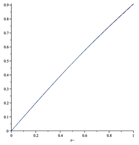
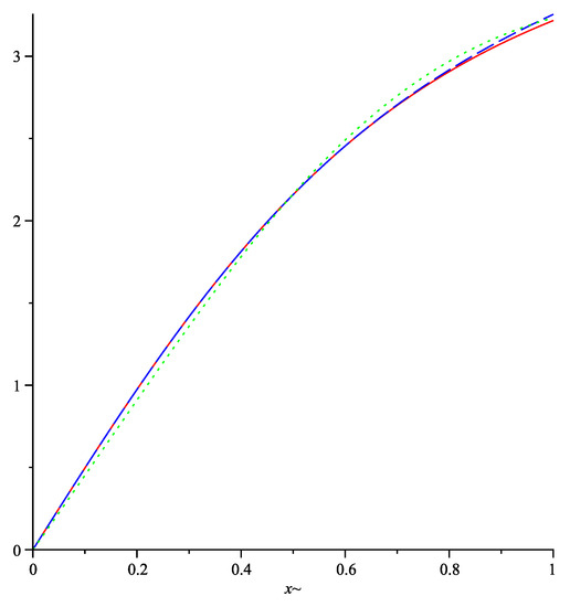
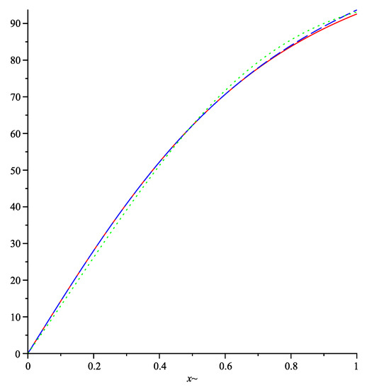
We can see that the quadrature rule (9) gives better approximations than the classical Milne’s rule (2). Moreover, comparing the absolute error of these quadrature rules relative to the exact value shows that (9) is much better than (2). For instance, for the first given function, (9) has an absolute error of 0.00015, whereas (2) has an absolute error of 0.00246. Similarly, for the second and third functions, (9) has an absolute error of 0.00041 and 0.07700, respectively. In contrast, (2) has an absolute error of 0.03740 and 1.089957, respectively. This shows that the quadrature rule (9) is much more precise than Milne’s rule (2) for this type of function. Therefore, we can conclude that (9) is a much better option for this integral approximation. Hence, (9) can be used as an alternative to Milne’s rule for obtaining more accurate values for an integral. This can be especially useful in cases where precision is paramount.

For further investigation, Figure 1 shows the area under the graph of $g\left(t\right)=\sqrt{\frac{4+t^7}{5+4t^2}}$, $t\in \left[0,1\right]$ (in red), the proposed quadrature (9) (in blue), and the classical Milne’s rule (in green). Clearly, the area under the blue colour coincides with the area under the $g\left(t\right)$ graph (in red). However, the area under the green colour (1) slightly differs from the area under the red and blue colours, meaning our approximation is better than the classical Milne’s quadrature rule. A similar analysis for $g\left(t\right)=\frac{\sqrt{25+t^7}}{1+2t^2+t^4}$ (Figure 2) and $g\left(t\right)=\frac{144+t^6}{1+2t^2+t^4}$ (Figure 3), could be stated by comparing the area under each graph (colour). The results demonstrate that our approximation is more accurate. Furthermore, it is computationally more efficient.

Figure 1. The area under $g\left(t\right)$ in red, The area under $g\left(t\right)$ using (9) in blue, and the area under $g\left(t\right)$ using Milne rule (1) in green.

Figure 2. The area under $g\left(t\right)$ in red, The area under $g\left(t\right)$ using (9) in blue, and the area under $g\left(t\right)$ using Milne rule (1) in green.

Figure 3. The area under $g\left(t\right)$ in red, The area under $g\left(t\right)$ using (9) in blue, and the area under $g\left(t\right)$ using Milne rule (1) in green.

On the other hand, if f does not have a bounded fourth derivative we cannot apply the classical Milne’s formula (2). Instead of that, we can use Formula (9) with $m=1$ and any appropriate norm; i.e., any norm that gives a small error estimate. Thus, we can still apply the rule

$$\begin{array}{c}\hfill {\int }_c^{d}g\left(s\right)ds\cong \frac{d-c}{3}\left[2g\left(\frac{3c+d}{4}\right)-g\left(\frac{c+d}{2}\right)+2g\left(\frac{c+3d}{4}\right)\right],\end{array}$$

(23)

even f does not have a bounded fourth derivative. Hence, our approach continues to use Milne’s rule (23), advantageous to Formula (9) with $m=1$. The following example shows several error estimates for (9).

Example 2.

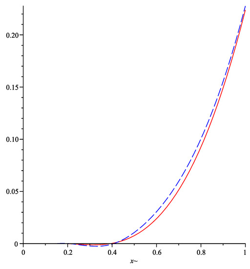
Consider $g\left(t\right)=t^{3}sin\left(\frac{1}{t}\right)$, $t\in \left[0,1\right]$. Therefore, the exact value of ${\int }_0^{1}g\left(t\right)dt$ is 0.223848. However, by applying (23), we obtain ${\int }_0^{1}g\left(t\right)dt\cong 0.227586$, with absolute error =0.003738. This difference shows that (23) can be an effective approximation for the integral of $g\left(t\right)$. Furthermore, it is an improvement over the exact value in terms of accuracy. In addition, only the first derivative is necessary to obtain the approximated value. There is no need for further bounded derivatives as they may not exist or be unbounded as in this example. Moreover, (23) is a computationally efficient solution as it eliminates the need to compute integrals of unbounded functions. This makes the approximation more convenient and efficient in terms of the computation time. Furthermore, the (23) approximation is more accurate than other numerical schemes, such as the midpoint rule, the trapezoid rule, Milne’s rule, or Simpson’s rule. These schemes require more evaluation and calculation. It is also more accurate than analytical methods, which may be difficult to implement in some cases. Additionally, it is more efficient than analytical methods in terms of the computation time. Hence, it is easier to calculate the first derivative than higher derivatives. This is significant as a higher order of accuracy can be achieved in a shorter amount of time. The more accurate the approximation, the less time is needed to solve the integral. This makes (23) a suitable choice for solving integrals that are difficult to calculate exactly. Using the (23) approximation also reduces the complexity of the integral. Since only the first derivative is needed, there is no need to calculate higher-order derivatives, which can be computationally expensive. Moreover, comparing the error estimates given by (13) with $l=1$ and $p=q=2$, we obtain ${∥g^{\prime }∥}_{\infty ,\left[0,1\right]}=1.98411$ and ${∥g^{\prime }∥}_{2,\left[0,1\right]}=1.18946$; hence,

$$\begin{array}{cc}\hfill \left|{\mathcal{E}}_1\left(g\right)\right|& \le \left\{\begin{array}{c}\frac{5}{24}{∥g^{\prime }∥}_{\infty ,\left[0,1\right]},\mathrm{if}{g}^{\prime }\in L^{\infty }[0,1]\hfill \\ \\ \frac{1}{3\sqrt{2}}{∥g^{\prime }∥}_{2,\left[0,1\right]},\mathrm{if}{g}^{\prime }\in L^p[0,1],\hfill \end{array}\right.\hfill \\ \hfill & =\left\{\begin{array}{c}0.413356,\mathrm{if}{g}^{\prime }\in L^{\infty }[c,d]\hfill \\ \\ 0.280359,\mathrm{if}{g}^{\prime }\in L^p[0,1].\hfill \end{array}\right.\hfill \end{array}$$

Since the error estimate given by the $L^2$-norm is less than the $L^{\infty }$-norm, the error given by the $L^2$-norm is better than the $L^{\infty }$-norm. Therefore, the $L^2$-norm can be used to estimate the error more accurately. We can confirm our approximated value by looking at Figure 4, which shows that the area under the green graph is close to the area under the red colour graph of $g\left(t\right)=t^{3}sin\left(\frac{1}{t}\right)$, $t\in \left[0,1\right]$. By comparing the two graphs we can confidently conclude that the approximated value is close to the exact value. This is because both the green and red graphs have a similar shape and the green graph appears to be slightly higher than the red graph, indicating that the approximated value is slightly larger than the actual value.

Figure 4. The area under $g\left(t\right)$ in red and (9) in blue.

6. Conclusions

In this work, a perturbed Milne’s quadrature formula was established. Namely, we have

$$\begin{array}{c}\hfill {\int }_c^{d}g\left(s\right)ds={\mathcal{M}}_m\left(g\right)+{\mathcal{E}}_m\left(g\right)\end{array}$$

for all $m\ge 1$, where ${\mathcal{M}}_m\left(g\right)$ is the perturbed Milne’s rule given by

$$\begin{array}{cc}\hfill & {\mathcal{M}}_m\left(g\right)\hfill \\ \hfill & :=\frac{d-c}{3}\left[2g\left(\frac{3c+d}{4}\right)-g\left(\frac{c+d}{2}\right)+2g\left(\frac{c+3d}{4}\right)\right]\hfill \\ \hfill & +\sum _{\ell =1}^{m-1}\frac{{\left(d-c\right)}^{\ell +1}}{\left(\ell +1\right)!}\left\{\left[{\left(\frac{5}{12}\right)}^{\ell +1}+{\left(\frac{1}{4}\right)}^{\ell +1}\right]\right.\hfill \\ \hfill & \left.\times \left[g^{(\ell )}\left(\frac{3c+d}{4}\right)+{\left(-1\right)}^{\ell }{g}^{(\ell )}\left(\frac{c+3d}{4}\right)\right]-\frac{\left({\left(-1\right)}^{\ell }+1\right)}{6^{\ell +1}}{g}^{(\ell )}\left(\frac{c+d}{2}\right)\right\},\hfill \end{array}$$

and ${\mathcal{E}}_m\left(g\right)$ is the error term given by

$$\begin{array}{c}\hfill {\mathcal{E}}_m\left(g\right)={\int }_c^{d}g\left(s\right)ds-{\mathcal{M}}_m\left(g\right)={\left(-1\right)}^m{\int }_c^d{\mathcal{K}}_m\left(s\right)g^{\left(m\right)}\left(s\right)ds\end{array}$$

for all $m\ge 1$. Furthermore, several error estimates involving $L^p$-bounds were proven. One of the most important advantages of our result is that it is verified for p-variation and Lipschitz functions (non-differentiable functions). Furthermore, since the classical Milne’s quadrature rule (2) cannot be applied either when the fourth derivative is unbounded or does not exist; therefore, the proposed quadrature in (13) with $m=1$ could be used alternatively. This is a very powerful indication that ensures that our result from (13) with $m=1$ is better than (2). It is not easy to determine the type of functions when (13) is better than (2)

Finally, it is convenient to note that other $L^p$-error estimates have been established. These estimates are useful if the fourth derivative is unbounded in the $L^{\infty }$-norm or the $L^p$-error estimate is less than the $L^{\infty }$-error estimate. This is especially worthwhile for certain classes of functions, such as those with singularities or discontinuities. Moreover, these error estimates allow us to compare the error between the $L^{\infty }$- and $L^p$-norms, and to determine which is more suitable for a particular problem. This case, however, gives very valuable and strong results that can be obtained using other $L^p$-norms, as shown in Example 2. This means that the error estimates can be applied to other $L^p$-norms and not just to $L^{\infty }$-norms, which increases the strength of our results since we can now apply the same estimates to a wider range of norms. This also gives us the advantage of being able to use different $L^p$-norms in our analysis, giving us more accurate results.

References

- Booth, A.D. Numerical Methods, 3rd ed.; Butterworth & Co.: Berkeley, CA, USA, 1966. [Google Scholar]
- Dragomir, S.S. On Simpson’s quadrature formula for mappings of bounded variation and applications. Tamkang J. Math. 1999, 30, 53–58. [Google Scholar] [CrossRef]
- Dragomir, S.S.; Agarwal, R.P.; Cerone, P. On Simpson’s inequality and applications. J. Inequal. Appl. 2000, 5, 533–579. [Google Scholar] [CrossRef]
- Sarikaya, M.Z.; Set, E.; Ozdemir, M.E. On new inequalities of Simpson’s type for s-convex functions. Comput. Math. Appl. 2010, 60, 2191–2199. [Google Scholar] [CrossRef]
- Sarikaya, M.Z.; Budak, H.; Erden, S. On new inequalities of Simpson’s type for generalized convex functions. Korean J. Math. 2019, 27, 279–295. [Google Scholar]
- Liu, Z. An inequality of Simpson type. Proc. R. Soc. Lond. Ser. A 2005, 461, 2155–2158. [Google Scholar] [CrossRef]
- Liu, Z. More on inequalities of Simpson type. Acta Math. Acad. Paedagog. Nyíregyházi. 2007, 23, 15–22. [Google Scholar]
- Shi, Y.; Liu, Z. Some sharp Simpson type inequalities and applications. Appl. Math. E-Notes 2009, 9, 205–215. [Google Scholar]
- Pečarić, J.; Varošanec, S. Simpson’s formula for functions whose derivatives belong to Lp spaces. Appl. Math. Lett. 2001, 14, 131–135. [Google Scholar] [CrossRef]
- Ujević, N. Two sharp inequalities of Simpson type and applications. Georgian Math. J. 2004, 1, 187–194. [Google Scholar] [CrossRef]
- Ujević, N. Sharp inequalities of Simpson type and Ostrowski type. Comp. Math. Appl. 2004, 48, 145–151. [Google Scholar] [CrossRef]
- Ujević, N. A generalization of the modified Simpson’s rule and error bounds. ANZIAM J. 2005, 47, E1–E13. [Google Scholar] [CrossRef]
- Ujević, N. New error bounds for the Simpson’s quadrature rule and applications. Comp. Math. Appl. 2007, 53, 64–72. [Google Scholar] [CrossRef]
- Alomari, M.W.; Guessab, A. Lp–error bounds of two and three-point quadrature rules for Riemann–Stieltjes integrals. Moroccan J. Pure Appl. Anal. 2018, 4, 33–43. [Google Scholar] [CrossRef]
- Alomari, M.W. Two-point quadrature rules for Riemann–Stieltjes integrals with Lp–error estimates. Moroccan J. Pure Appl. Anal. 2018, 4, 94–110. [Google Scholar] [CrossRef]
- Alomari, M.W. Two-point Ostrowski’s inequality. Results Math. 2017, 72, 1499–1523. [Google Scholar] [CrossRef]
- Alomari, M.W. On Beesack–Wirtinger inequality. Results Math. 2017, 72, 1213–1225. [Google Scholar] [CrossRef]
- Alomari, M.W. Two–point Ostrowski and Ostrowski–Grüss type inequalities with applications. J. Anal. 2020, 28, 623–661. [Google Scholar] [CrossRef]
- Alomari, M.W. New sharp inequalities of Ostrowski and generalized trapezoid type for the Riemann–Stieltjes integrals and applications. Ukr. Math. J. 2013, 65, 895–916. [Google Scholar] [CrossRef][Green Version]
- Alomari, M.W.; Dragomir, S.S. A three-point quadrature rule for the Riemann-Stieltjes integral. Southeast Asian Bull. J. Math. 2018, 42, 1–14. [Google Scholar]
- Barnett, N.S.; Dragomir, S.S.; Gomma, I. A companion for the Ostrowski and the generalised trapezoid inequalities. Math. Comput. Model. 2009, 50, 179–187. [Google Scholar] [CrossRef]
- Barnett, N.S.; Cheung, W.-S.; Dragomir, S.S.; Sofo, A. Ostrowski and trapezoid type inequalities for the Stieltjes integral with Lipschitzian integrands or integrators. Comput. Math. Appl. 2009, 57, 195–201. [Google Scholar] [CrossRef][Green Version]
- Cerone, P.; Dragomir, S.S. New Bounds for the Three-Point Rule Involving the Riemann-Stieltjes Integrals. In Advances in Statistics Combinatorics and Related Areas; Gulati, C., Lin, Y., Mishra, S., Rayner, J., Eds.; World Science Publishing: Hackensack, NJ, USA, 2002; pp. 53–62. [Google Scholar]
- Cerone, P.; Dragomir, S.S. Approximating the Riemann–Stieltjes integral via some moments of the integrand. Math. Comput. Model. 2009, 49, 242–248. [Google Scholar] [CrossRef][Green Version]
- Alomari, M.W.; Liu, Z. New error estimations for the Milne’s quadrature formula in terms of at most first derivatives. Konuralp J. Math. 2013, 1, 17–23. [Google Scholar]
- Milovanović, G.V. Ostrowski type inequalities and some selected quadrature formulae. Appl. Anal. Discrete Math. 2021, 15, 151–178. [Google Scholar] [CrossRef]
- Qawasmeh, T.; Hatamleh, R. A new contraction based on H-simulation functions in the frame of extended b-metric spaces and application. Inter. J. Elec. Comp. Eng. 2023, 13, 4212–4221. [Google Scholar] [CrossRef]
- Qazza, A.; Hatamleh, R. The existence of a solution for semi-linear abstract differential equations with infinite B-chains of the characteristic. Inter. J. Appl. Math. 2018, 31, 611. [Google Scholar] [CrossRef]
- Salah, E.; Saadeh, R.; Qazza, A.; Hatamleh, R. Direct power series approach for solving nonlinear initial Value problems. Axioms 2023, 12, 111. [Google Scholar] [CrossRef]
- Cerone, P.; Dragomir, S.S. Midpoint–type rules from an inequalities point of view. In Handbook of Analytic Computational Methods in Applied Mathematics; Anastsssiou, G., Ed.; CRC Press: New York, NY, USA, 2000; pp. 135–200. [Google Scholar]
- Cerone, P.; Dragomir, S.S. Trapezoidal–type rules from an inequalities point of view. In Handbook of Analytic Computational Methods in Applied Mathematics; Anastsssiou, G., Ed.; CRC Press: New York, NY, USA, 2000; pp. 65–134. [Google Scholar]
- Cerone, P.; Dragomir, S.S.; Roumeliotis, J.; Šunde, J. A new generalization of the trapezoid formula for n-time differentiable mappings and applications. Demonstr. Math. 2000, 33, 719–736. [Google Scholar] [CrossRef]
- Guessab, A.; Schmeisser, G. Sharp integral inequalities of the Hermite-Hadamard type. J. Approx. Theory 2002, 115, 260–288. [Google Scholar] [CrossRef]
- Kovač, S.; Pečarić, J. Generalization of an integral formula of Guessab and Schmeisser. Banach J. Math. Anal. 2011, 5, 1–18. [Google Scholar] [CrossRef]
- Liu, Z. Some companions of an Ostrowski type inequality and applications. J. Ineq. Pure Appl. Math. 2009, 10, 52. [Google Scholar]
- Sofo, A. Integral Inequalities for n-Times Differentiable Mappings, Chapter II. In Ostrowski Type Inequalities and Applications in Numerical Integration; Dragomir, S.S., Rassias, T.M., Eds.; Kluwer Academic Publishers: Dordrecht, The Netherlands, 2002. [Google Scholar]
- Ujević, N. A generalization of Ostrowski’s inequality and applications in numerical integration. Appl. Math. Lett. 2004, 17, 133–137. [Google Scholar] [CrossRef]
- Davis, P.J. Interpolation and Approximation; Dover: Mineola, NY, USA, 1975. [Google Scholar]
- Dedić, L.; Matić, M.; Pečarić, J. On Euler–Maclaurin formulae. Math. Inequal. Appl. 2003, 6, 247–275. [Google Scholar] [CrossRef]
- Dedić, L.; Matić, M.; Pečarić, J. On dual Euler–Simpson formulae. Bull. Belg. Math. Soc. 2001, 8, 479–504. [Google Scholar] [CrossRef]
- Dedić, L.; Matić, M.; Pečarić, J. On Euler–Simpson formulae. Pan. Am. Math. J. 2001, 11, 47–64. [Google Scholar]
- Dedić, L.; Matić, M.; Pečarić, J. On generalizations of Ostrowski inequality via some Euler–type identities. Math. Inequal. Appl. 2000, 3, 337–353. [Google Scholar] [CrossRef]
- Hatamleh, R.; Zolotarev, V.A. Triangular Models of Commutative Systems of Linear Operators Close to Unitary Ones. Ukr. Math. J. 2016, 68, 791–811. [Google Scholar] [CrossRef]
- Franjić, I.; Pečarić, J.; Perić, I. General three–point quadrature formulas of Euler type. ANZIAM J. 2011, 52, 309–317. [Google Scholar] [CrossRef]
- Franjić, I.; Perić, I.; Pečarić, J. Estimates for the Gauss four-point formula for functions with low degree of smoothness. Appl. Math. Lett. 2007, 20, 1–6. [Google Scholar] [CrossRef][Green Version]
- Franjić, I.; Pečarić, J. On corrected Bullen-Simpson’s 3/8 inequality. Tamkang J. Math. 2006, 37, 135–148. [Google Scholar] [CrossRef]
- Franjić, I.; Pečarić, J.; Perić, I. General Euler–Boole’s and dual Euler–Boole’s formulae. Math. Ineq. Appl. 2005, 8, 287–303. [Google Scholar]
- Franjić, I.; Pečarić, J. Corrected Euler–Maclaurin’s formulae. Rendi. Circolo Mate. Palermo 2005, 54, 259–272. [Google Scholar] [CrossRef]
- Kythe, P.K.; Schäferkotter, M.R. Handbook of Computational Methods for Integration; Chapman & HallL/CRC, A CRC Press Company: London, UK, 2005. [Google Scholar]
- Mastroianni, G.; Milovanović, G.V. Interpolation Processes–Basic Theory and Applications; Springer Monographs in Mathematics; Springer: Berlin/Heidelberg, Germany, 2008. [Google Scholar]
Disclaimer/Publisher’s Note: The statements, opinions and data contained in all publications are solely those of the individual author(s) and contributor(s) and not of MDPI and/or the editor(s). MDPI and/or the editor(s) disclaim responsibility for any injury to people or property resulting from any ideas, methods, instructions or products referred to in the content. |
© 2023 by the authors. Licensee MDPI, Basel, Switzerland. This article is an open access article distributed under the terms and conditions of the Creative Commons Attribution (CC BY) license (https://creativecommons.org/licenses/by/4.0/).