Typical = Random

Abstract

This expository paper advocates an approach to physics in which “typicality” is identified with a suitable form of algorithmic randomness. To this end various theorems from mathematics and physics are reviewed. Their original versions state that some property $\Phi \left(x\right)$ holds for P-almost all $x\in X$, where P is a probability measure on some space X. Their more refined (and typically more recent) formulations show that $\mathrm{\Phi }\left(x\right)$ holds for all P-random $x\in X$. The computational notion of P-randomness used here generalizes the one introduced by Martin-Löf in 1966 in a way now standard in algorithmic randomness. Examples come from probability theory, analysis, dynamical systems/ergodic theory, statistical mechanics, and quantum mechanics (especially hidden variable theories). An underlying philosophical theme, inherited from von Mises and Kolmogorov, is the interplay between probability and randomness, especially: which comes first?

1. Introduction

The introduction of probability in statistical mechanics in the 19th century by Maxwell and Boltzmann raised questions about both the meaning of this concept by itself and its relationship to randomness and entropy [1,2,3,4,5]. Roughly speaking, both initially felt that probabilities in statistical mechanics were dynamically generated by particle trajectories, a view which led to ergodic theory. But subsequently Boltzmann [6] introduced his counting arguments as a new start; these led to his famous formula for the entropy $S=klogW$ on his gravestone in Vienna, i.e.,

probability first, entropy second.

This was turned on its head by Einstein [7], who had rediscovered much of statistical mechanics by himself in his early work, always stressing the role of fluctuations. He expressed the probability of energy fluctuations in terms of entropy seen as a primary concept. This suggests:

entropy first, probability second.

From the modern point of view of large deviation theory [8,9,10,11], what happens is that for finite N some stochastic process $\left(X_N\right)$ fluctuates around its limiting value $\overline{X}$ as $N\to \infty$ (if it has one), and, under favorable circumstances that often obtain in statistical mechanics, the “large” i.e., $O\left(1\right)$ fluctuations (as opposed to the $O(1/\sqrt{N})$ fluctuations, which are described by the central limit theorem [12]) can be computed via an entropy function $S\left(x\right)$ whose argument x lies in the (common) codomain $\mathcal{X}$ of $X_N:\Omega \to \mathcal{X}$. Since the domain $\Omega$ of $X_N$ carries a probability measure to begin with, it seems an illusion that entropy could be defined without some prior notion of probability.

Similar questions may be asked about the connection between probability and randomness (and, closing the triangle, of course also about the relationship between randomness and entropy). First, in his influential (but flawed) work on the foundations of probability, von Mises [13,14] initially defined randomness through a Kollektiv (which, with hindsight, was a precursor to a random sequence). From this, he extracted a notion of probability via asymptotic relative frequencies. See also [5,15,16,17]. Von Plato [5] (p. 190) writes that ‘He [von Mises] was naturally aware of the earlier attempts of Einstein and others at founding statistical physics on classical dynamics’ and justifies this view in his Section 6.3. Thus:

randomness first, probability second.

Kolmogorov [18], on the other hand, (impeccably) defined probability first (via measure theory), in terms of which he hoped to understand randomness. In other words, his (initial) philosophy was:

probability first, randomness second.

Having realized that this was impossible, thirty years later Kolmogorov [19,20] arrived at the concept of randomness named after him, using tools from computer and information science that actually had roots in in the work of von Mises (as well as of Turing, Shannon, and others). See [5,15,21,22,23,24]. So:

Kolmogorov randomness first, measure-theoretic probability second.

But I will argue that even Kolmogorov randomness seems to rely on some prior concept of probability, see Section 3 and in particular the discussion surrounding Theorem 4; and this is obviously the case for Martin-Löf randomness, both in its original form for binary sequences (which is essentially equivalent to Kolmogorov randomness as extended from finite strings to infinite sequences, see Theorem 3) and in its generalizations (see Section 3). So I will defend the view that after all we have

some prior probability measure first, Martin-Löf randomness second.

In any case, there isn’t a single concept of randomness [25], not even within the algorithmic setting [26]; although the above slogan probably applies to most of them.

Motivated by the above discussion and its potential applications to physics, the aim of this paper is to review the interplay between probability, (algorithmic) randomness, and entropy via examples from probability itself, analysis, dynamical systems and (Boltzmann-style) statistical mechanics, and quantum mechanics. Some basic relations are explained in the next Section 2. In Section 3 I review algorithmic randomness beyond binary sequences. Section 4 introduces some key “intuition pumps”: these are results in which ‘for P-almost every x: $\Phi \left(x\right)$’ in some “classical” result can be replaced by ‘for all P-random x: $\Phi \left(x\right)$’ in an “effective” counterpart thereof; this replacement may even be seen as the essence of algorithmic randomness. In Section 5 I apply this idea to statistical mechanics, and close in Section 6 with some brief comments on quantum mechanics. The paper closes with a brief summary.

2. Some Background on Entropy and Probability

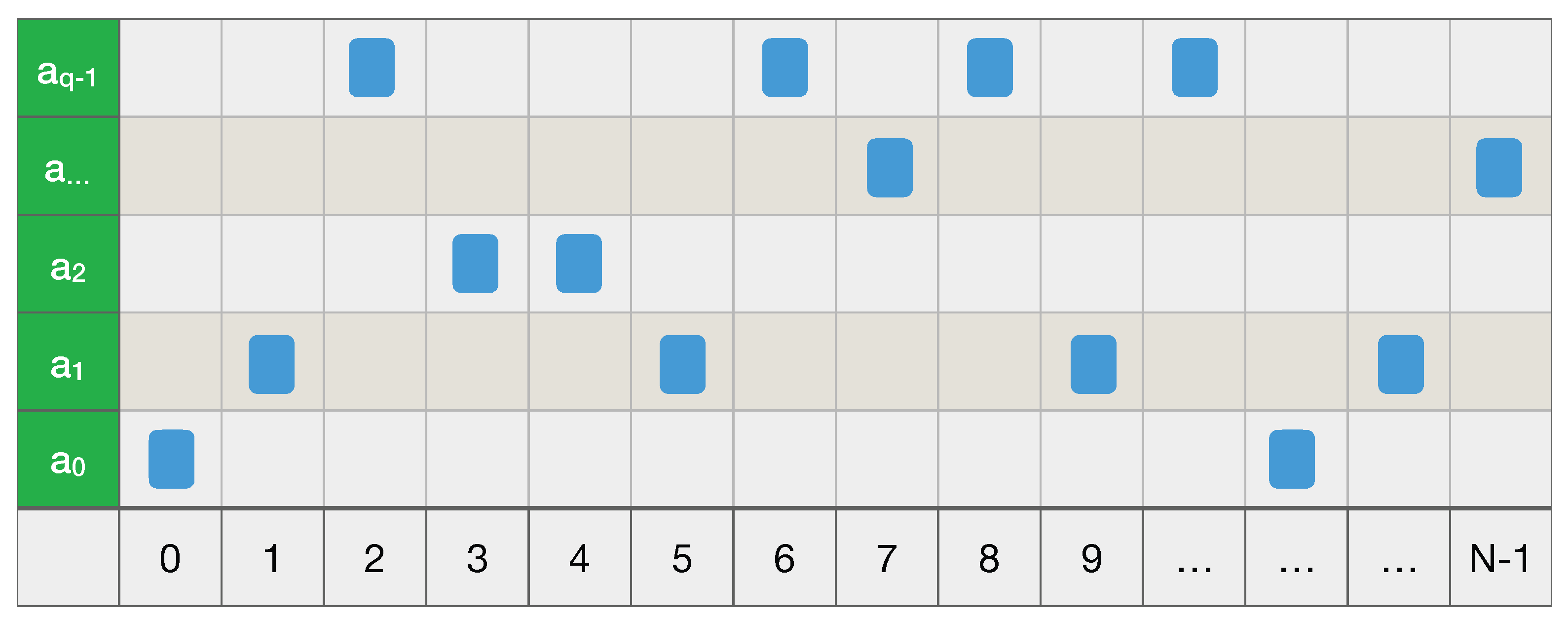
Consider Figure 1, which connects and illustrates the main examples in this paper.

Figure 1. Sample configuration on N objects each of which can be in q different states.

Here $N\in \mathbb{N}$ is meant to be some large natural number, whereas $q\in \{2,3,\dots \}$, the cardinality of

$$A=\{a_0,\dots ,a_{q-1}\},$$

(1)

could be anything (finite), but is small ($q=2$) in the already interesting case of binary strings. In what follows, $A^N$ is the set of all functions $\sigma :N\to A$, where

$$N=\{0,1,\dots ,N-1\},$$

(2)

as usual in set theory. Such a function is also called a string over A, having length

$$\ell \left(\sigma \right)\equiv \left|\sigma \right|=N.$$

(3)

We write either $\sigma \left(n\right)$ or ${\sigma }_n$ for its value at $n\in N$, and may write $\sigma$ as ${\sigma }_0{\sigma }_1\cdots {\sigma }_{N-1}$. In particular, if $A=2=\{0,1\}$, then $\sigma$ is a binary string. I write

$$A^{\ast }\equiv A^{<\omega }=\bigcup _{N\in \mathbb{N}}{A}^N,$$

(4)

so that for example $2^{\ast }={\bigcup }_{N\in \mathbb{N}}{2}^N$ is the set of all binary strings. Thus a (binary) string $\sigma$ is finite, whereas a (binary) sequence s is infinite. The set of all binary sequences is denoted by $2^{\omega }$, and likewise $A^{\omega }$ consists of all functions $s:\mathbb{N}\to A$. For $s\in A^{\omega }$, I write $s_{|N}$ for $s_0{s}_1\cdots s_{N-1}\in A^N$, to be sharply distinguished from $s_n\equiv s\left(n\right)\in A$. Using this notation, I now review various ways of looking at Figure 1. Especially in the first two items below it is hard to avoid overlap with e.g., the reviews [27,28], which I recommend for further information.

• In statistical mechanics as developed by Boltzmann in 1877 [6], and more generally in what one might call “Boltzmann-style statistical mechanics”, which is based on typicality arguments [29], N is the number of (distinguishable) particles under consideration, and A could be a finite set of single-particle energy levels. More generally, $a\in A$ is some property each particle may separately have, such as its location in cell $X_a$ relative to some partition

  $$X=\underset{a\in A}{⨆}{X}_a$$

  (5)

  of the single-particle phase space or configuration space X accessible to each particle. Here $X_a\subset X$ and different $X_a$ are disjoint, which fact is expressed by the symbol ⨆ in (5). One might replace ⨆ by ⋃ as long as one knows that the subsets $X_a$ are mutually disjoint (and measurable as appropriate). The microstate $\sigma \in A^N$ is a function

  $$\sigma :\{0,1,\dots ,N-1\}\to A$$

  (6)

  that specifies which property (among the possibilities in A) each particle has. Thus also spin chains fall under this formalism, where ${\sigma }_n\in A$ is some internal degree of freedom at site n. In Boltzmann-style arguments it is often assumed that each microstate is equally likely, which corresponds to the probability $P_f^N$ on $A^N$ defined by

  $$P_f^N\left(\left\{\sigma \right\}\right)={\left|A\right|}^{-N}=q^{-N},$$

  (7)

  for each $\sigma \in A^N$. This is the Bernoulli measure on $A^N$ induced by the flat prior $p=f$ on A,

  $$f\left(a\right)=1/q,$$

  (8)

  for each $a\in A$. More generally, $P_p^N$ is the Bernoulli measure on $A^N$ induced by some probability distribution p on A; that is, the product measure of N copies of p; some people write $P_p^N=p^{\times N}$. This extends to the idealized case $A^{\omega }$, as follows. For $\sigma \in A^N$ we define

  $$\left[\sigma \right]:=\sigma A^{\omega }=\{s\in A^{\omega }\mid \sigma \prec s\},$$

  (9)

  where $\sigma \prec s$ means that $s=\sigma \tau$ for some $\tau \in A^{\omega }$ (in words: $\sigma \in A^{\ast }$ is a prefix of $s\in A^{\omega }$). On these basic measurable (and open) sets we define a probability measure $P_p^{\omega }$ by

  $$P_p^{\omega }\left(\left[\sigma \right]\right)=P_p^N\left(\sigma \right).$$

  (10)

  In particular, if $\sigma \in A^N$, then its unbiased probability is simply given by

  $$P_f^{\omega }\left(\left[\sigma \right]\right)={\left|A\right|}^{-N}.$$

  (11)

  It is important to keep track of p even if it is flat: making no (apparent) assumption (which $p=f$ is often taken to be) is an important assumption! For example, Boltzmann’s famous counting argument [6] really reads as follows [30,31,32,33]. The formula

  $$S=klogW$$

  (12)

  on Boltzmann’s grave should more precisely be something like

  $$S_B^N\left(\mu \right)=log{W}^N\left(\mu \right),$$

  (13)

  where I omit the constant k and take $\mu \in \mathrm{Prob}\left(A\right)$ to be the relevant argument of the (extensive) Boltzmann entropy $S_B^N$ (see below). Furthermore, $W^N\left(\mu \right)$ is the probability (“Wahrscheinlichkeit”) of $\mu$, which Boltzmann, assuming the flat prior (8) on A, took as

  $$W^N\left(\mu \right)=\frac{N\left(\mu \right)}{{\left|A\right|}^N},$$

  (14)

  where $N\left(\mu \right)$ is the number of microstates $\sigma \in A^N$ whose corresponding empirical measure

  $$L_N\left(\sigma \right)=\frac{1}{N}\sum _{n=0}^{N-1}{\delta }_{\sigma \left(n\right)},$$

  (15)

  equals $\mu$. Here, for any $b\in A$, ${\delta }_b\in \mathrm{Prob}\left(A\right)$ is the point measure at b, i.e., ${\delta }_b\left(a\right)={\delta }_{ab}$, the Kronecker delta. The number $N\left(\mu \right)$ is only nonzero if $\mu \in {\mathrm{Prob}}_N\left(A\right)$, which consists of all probability distributions $\nu$ on A that arise as $\nu =L_N\left(\sigma \right)$ for some $\sigma \in A^N$. This, in turn, means that $\nu \left(a\right)={\nu }^{\prime }\left(a\right)/N$ for some ${\nu }^{\prime }\left(a\right)\in \{0,\dots ,N\}$, with ${\sum }_{a\in A}{\nu }^{\prime }\left(a\right)=N$. In that case,

  $$N\left(\mu \right)=\frac{N!}{{\prod }_{a\in A}({\mu }^{\prime }\left(a\right)!)}.$$

  (16)

  The term ${\left|A\right|}^{-N}$ in (14) of course equals $P^N\left(\sigma \right)$ for any $\sigma \in A^N$ and hence certainly for any $\sigma$ for which $L_N\left(\sigma \right)=\mu$. For such $\sigma$, for general Bernoulli measures $P_p$ on $A^N$ we have

  $$P_p^N\left(\sigma \right)=e^{N{\sum }_{a\in A}\mu \left(a\right)logp\left(a\right)}=e^{-N\left(h\right(\mu )+I(\mu \left|p\right))},$$

  (17)

  in terms of the Shannon entropy and the Kullback–Leibler distance (or divergence), given by

  $$\begin{array}{cc}\hfill h\left(\mu \right)& :=-\sum _{a\in A}\mu \left(a\right)log\mu \left(a\right);\hfill \end{array}$$

  (18)

  $$\begin{array}{cc}\hfill I\left(\mu \right|p)& :=\sum _{a\in A}\mu \left(a\right)log\left(\frac{\mu \left(a\right)}{p\left(a\right)}\right),\hfill \end{array}$$

  (19)

  respectively. These are simply related: for the flat prior (8) we have

  $$\begin{array}{c}\hfill I\left(\mu \right|f)=-h(\mu )+log|A|.\end{array}$$

  (20)

  In general, computing $S_B^N\left(\mu \right)$ from (13) and, again assuming $L_N\left(\sigma \right)=\mu$, we obtain

  $$W^N\left(\mu \right)=P_p^N(L_N=\mu )=N\left(\mu \right)P_p^N\left(\sigma \right)=\frac{N!e^{-N\left(h\right(\mu )+I(\mu \left|p\right))}}{{\prod }_{a\in A}({\mu }^{\prime }\left(a\right)!)},$$

  (21)

  from which Stirling’s formula (or the technique in [Section 2.1] in [31]) gives

  $$s_B\left(\mu \right|p):=\underset{N\to \infty }{lim}\frac{S_B^N\left({\mu }_N\right)}{N}=-I\left(\mu \right|p),$$

  (22)

  where ${\mu }_N\in {\mathrm{Prob}}_N\left(A\right)$ is any sequence of probability distributions on A that (weakly) converges to $\mu \in \mathrm{Prob}\left(A\right)$, i.e., the variable in $s_B(·|p)$. For the flat prior (8), Equation (20) yields

  $$s_B\left(\mu \right|f)=h\left(\mu \right)-log\left|A\right|.$$

  (23)

  As an aside, note that the Kullback–Leibler distance or relative entropy (19) is defined more generally for probability measures $\mu$ and p on some measure space $(A,\Sigma )$. As usual, we write $\mu \ll p$ iff $\mu$ is absolutely continuous with respect to p, i.e., $p\left(B\right)=0$ implies $\mu \left(B\right)=0$ for $B\in \Sigma$. In that case, the Radon–Nikodym derivative $d\mu /dp$ exists, and one has

  $$I\left(\mu \right|p):={\int }_{A}dp\frac{d\mu }{dp}log\left(\frac{d\mu }{dp}\right).$$

  (24)

  If $\mu$ is not absolutely continuous with respect to p, one puts $I\left(\mu \right|p):=\infty$. The nature of the empirical measure (15) and the Kullback–Leibler distance (19) comes out well in hypothesis testing. In order to test the hypothesis $H_0$ that $\mu ={\mu }_0$ by an N-fold trial $\sigma \in A^N$, one accepts $H_0$ iff $I\left(L_N\left(\sigma \right)\right|{\mu }_0)<\eta$, for some $\eta >0$. This test is optimal in the sense of Hoeffding [Section 3.5] in [31]. But let us return to the main story.
  The stochastic process $X_N:\Omega \to \mathcal{X}$ whose large fluctuations are described by (22) is

  $$\begin{array}{ccccccc}\hfill \mathcal{X}=\mathrm{Prob}\left(A\right);& \hfill & \hfill \Omega =A^{\omega };& \hfill & \hfill P=P_p^{\omega };& \hfill & \hfill X_N=L_N.\end{array}$$

  (25)

  Then $L_N\to p$ almost surely, and large fluctuations around this value are described by

  $$\begin{array}{c}\hfill \underset{N\to \infty }{lim}\frac{1}{N}log{P}_p^N(L_N\in \Gamma )=-I(\Gamma |p):=-\underset{\mu \in \Gamma }{inf}I\left(\mu \right|p)=\underset{\mu \in \Gamma }{sup}{s}_B\left(\mu \right|p),\end{array}$$

  (26)

  where $\Gamma \subset \mathrm{Prob}\left(A\right)$ is open, or more generally, is such that $\Gamma \subseteq \overline{\mathrm{int}(\Gamma )}$. Less precisely,

  $$\begin{array}{ccc}\hfill P_p^N(L_N\in \Gamma )\approx e^{-NI(\Gamma |p)}& \hfill & \hfill \mathrm{as}N\to \infty ,\end{array}$$

  (27)

  which implies that $P_p^N(L_N\in \Gamma )\approx 1$ if $p\in \Gamma$, whereas $P_p^N(L_N\in \Gamma )$ is exponentially damped if $p\notin \Gamma$. Note that the rate function $\mu \mapsto I\left(\mu \right|p)$ defined in (19) and (26) is convex and positive, whereas the entropy (22) is concave and negative. Thus the former is to be minimized, its infimum (even minimum) over $\mu \in \mathrm{Prob}\left(A\right)$ being zero at $\mu =p$, whereas the latter is to be maximized, its supremum (even maximum) at the same value being zero. The first term in (23) hides the negativity of the Boltzmann entropy (here for a flat prior), but the second term drives it below zero. Positivity of $I\left(\mu \right|p)$ follows from (or actually is) the Gibbs inequality. Equation (26) is a special case of Sanov’s theorem, which works for arbitrary Polish spaces (instead of our finite set A); see [8,31]. Einstein [7] computes the probability of large fluctuations of the energy, rather than of the empirical measure, as Boltzmann did in 1877 [6], but these are closely related.
  Interpreting A as a set of energy levels, the relevant stochastic process $X_N:\mathrm{\Omega }\to \mathcal{X}$ still has $\Omega$ and P as in (25), but this time $X_N:\mathrm{\Omega }\to \mathbb{R}$ is the average energy, defined by

  $$X_N\left(\sigma \right)\equiv E_N\left(\sigma \right)=\frac{1}{N}\sum _{n=0}^{N-1}\sigma \left(n\right).$$

  (28)

  This makes the relevant entropy $s_C$ (which is the original entropy from Clausius-style thermodynamics!) a function of $u\in \mathbb{R}$, interpreted as energy: instead of (26), one obtains

  $$\begin{array}{cc}\hfill \underset{N\to \infty }{lim}\frac{1}{N}log{P}_p^N(E_N\in \Delta )& =\underset{u\in \Delta }{sup}{s}_C\left(u\right|p);\hfill \end{array}$$

  (29)

  $$\begin{array}{cc}\hfill s_C\left(u\right|p)& :=\underset{\mu \in \mathrm{Prob}\left(A\right)}{sup}\left\{s_B\left(\mu \right|p)\mid \sum _{a\in A}\mu \left(a\right)·a=u\right\},\hfill \end{array}$$

  (30)

  which “maximal entropy principle” is a special case of Cramér’s theorem [8,31]. If $\overline{u}={\sum }_{a\in A}p\left(a\right)·a$ lies in $\Delta \subset \mathbb{R}$, then $log{P}_p^N(E_N\in \Delta )\approx 1$. If not, this probability is exponentially small in N. To obtain the classical thermodynamics of non-interacting particles [32], one may add that the free energy

  $$f\left(\beta \right|p)=log\left(\sum _{a\in A}p\left(a\right)e^{-\beta a}\right)$$

  (31)

  is essentially the Fenchel transform [34] of the entropy $s_C\left(u\right|p)$, in that

  $$\begin{array}{ccc}\hfill \beta f\left(\beta \right|p)=\underset{u\in \mathbb{R}}{inf}\{\beta u-s_C\left(u\right|p)\};& \hfill & \hfill s_C\left(u\right|p)=\underset{\beta \in \mathbb{R}}{inf}\{\beta u-\beta f\left(\beta \right|p)\}.\end{array}$$

  (32)

  For $\beta >0$, the first equality is a refined version of “$F=E-TS$”.
• In information theory as developed by Shannon [35] (see also [36,37,38]) the “N” in our diagram is the number of letters drawn from an alphabet A by sampling a given probability distribution $p\in \mathrm{Prob}\left(A\right)$, the space of all probability distributions on A. So each microstate $\sigma \in A^N$ is a word with N letters. The entropy of p, i.e.,

  $$h_2\left(p\right):=-\sum _{a\in A}p\left(a\right){log}_{2}p\left(a\right)=\sum _{a\in A}p\left(a\right)I_2\left(a\right),$$

  (33)

  plays a key role in Shannon’s approach. It is the expectation value $h_2\left(p\right)={⟨I⟩}_p$ of the function

  $$I_2\left(a\right):=-{log}_{2}p\left(a\right),$$

  (34)

  interpreted as the information contained in $a\in A$, relative to p. This interpretation is evident for the flat distribution $p=f$ on an alphabet with $\left|A\right|=2^n$ letters, in which case $I_2\left(a\right)=n$ for each $a\in A$, which is the minimal number of bits needed to (losslessly) encode a. The general case is covered by the noiseless coding theorem for prefix (or uniquely decodable) codes. A map $C:A\to 2^{\ast }$ is a prefix code if it is injective and $C\left(a\right)$ is never a prefix of $C\left(b\right)$ for any $a,b\in A$, that is, there is no $\tau \in 2^{\ast }$ such that $C\left(b\right)=C\left(a\right)\tau$. A prefix code is uniquely decodable. Let $C:A\to 2^{\ast }$ be a prefix code, let $\ell \left(C\right(a\left)\right)$ be the length of the codeword $C\left(a\right)$, with expectation

  $$L(C,p)=\sum _{a\in A}p\left(a\right)\ell \left(C\left(a\right)\right).$$

  (35)

  An optimal code minimizes this. Then:
  • Any prefix code satisfies $h_2\left(p\right)\le L(C,p)$;
  • There exists an optimal prefix code C, which satisfies $L(C,p)\le h_2\left(p\right)+1$.
  • One has $h_2\left(p\right)=L(C,p)$ iff $\ell \left(C\left(a\right)\right)=I_2\left(a\right)$ for each $a\in A$ (if this is possible).
  Of course, the equality $\ell \left(C\left(a\right)\right)=I_2\left(a\right)$ can only be satisfied if $p\left(a\right)=2^{-k}$ for some integer $k\in \mathbb{N}$. Otherwise, one can find a code for which $\ell \left(C\left(a\right)\right)=\left[I_2\left(a\right)\right]$, the smallest integer $\ge I_2\left(a\right)$. See e.g., [Section 5.4] in [36].
  Thus the information content $I_2\left(a\right)$ is approximately the length of the code-word $C\left(a\right)$ in some optimal coding C. Passing to our case of interest of N-letter words over A, in case of a memoryless source one simply has the Bernoulli measure $P_p^N$ on $A^N$, with entropy

  $$H_2\left(P_p^N\right)=-\sum _{\sigma \in A^N}{P}_p^N\left(\sigma \right){log}_2{P}_p^N\left(\sigma \right)=N{h}_2\left(p\right).$$

  (36)

  Extending the letter-code $C:A\to 2^{\ast }$ to a word-code $C^N:A^N\to 2^{\ast }$ by concatenation, i.e., $C^N(a_{i_0}\cdots a_{i_{N-1}})=C\left(a_{i_0}\right)\cdots C\left(a_{i_{N-1}}\right)$, and replacing $L(C^N,P_p^N)$, which diverges as $N\to \infty$, by the average codeword length per symbol $L(C^N,P_p^N)/N$, an optimal code C satisfies

  $$\underset{N\to \infty }{lim}\frac{L(C^N,P_p^N)}{N}=h_2\left(p\right).$$

  (37)

  In what follows, the Asymptotic Equipartition Property or AEP will be important. In its (probabilistically) weak form, which is typically used in information theory, this states that

  $$\begin{array}{c}\hfill {\forall }_{\epsilon >0}\underset{N\to \infty }{lim}{P}_p^N\left(\left\{\sigma \in A^N\mid P_p^N\left(\sigma \right)\in [2^{-N(h_2\left(p\right)+\epsilon )},2^{-N(h_2\left(p\right)-\epsilon )}]\right\}\right)=1.\end{array}$$

  (38)

  Its strong form, which is the (original) Shannon–McMillan–Breiman theorem, reads

  $$\begin{array}{c}\hfill P_p^{\omega }\left(\left\{s\in A^{\omega }\mid \underset{N\to \infty }{lim}-\frac{1}{N}{log}_2{P}_p^N\left(s_{|N}\right)=h_2\left(p\right)\right\}\right)=1.\end{array}$$

  (39)

  Either way, the idea is that for large N, with respect to $P_p^N$ “most” strings $\sigma \in A^N$ have “almost” the same probability $2^{-N{h}_2\left(p\right)}$, whilst the others are negligible [lecture 2] in [30]. For $A=2$ with flat prior $p=f$ this yields a tautology: all strings $\sigma \in 2^N$ have $P_f^N\left(\sigma \right)=2^{-N}$. See e.g., [Sections 3.1 and 16.8] in [36]. The strong form follows from ergodic theory, cf. (53).
• In dynamical systems along the lines of the ubiquitous Kolmogorov [39], one starts with a triple $(X,P,T)$, where X–more precisely $(X,\Sigma )$, but I usually suppress the $\sigma$-algebra $\Sigma$–is a measure space, P is a probability measure on X (more precisely, on $\Sigma$), and $T:X\to X$ is a measurable (but not necessarily invertible) map, required to preserve P in the sense that $P\left(T^{-1}B\right)=P\left(B\right)$ for any $B\in \Sigma$. A measurable coarse-graining (5) defines a map

  $$\begin{array}{ccc}\hfill \xi :X\to A^{\omega };& \hfill & \hfill \xi {\left(x\right)}_n=a\in A\mathrm{iff}{T}^{n}x\in X_a,\end{array}$$

  (40)

  in terms of which the given triple $(X,P,T)$ is coarse-grained by a new triple $(A^{\omega },{\xi }_{\ast }P,S)$. Here ${\xi }_{\ast }P\left(B^{\prime }\right)=P\left({\xi }^{-1}B\right)$ is the induced probability on $A^{\omega }$, whilst S is the (unilateral) shift

  $$\begin{array}{ccc}\hfill S:A^{\omega }\to A^{\omega };& \hfill & \hfill {\left(Ss\right)}_n:=s_{n+1}(n=0,1,\dots )\end{array}$$

  (41)

  A fine-grained path $(x,Tx,T^{2}x,\dots )\in X^{\omega }$ is coarse-grained to $\xi \left(x\right)\in A^{\omega }$, and truncating the latter at $t=N-1$ gives $\xi {\left(x\right)}_{|N}\in A^N$. Hence the configuration in Figure 1 states that our particle starts from $x\in X_{a\left(0\right)}\subset X$ at $t=0$, moves to $Tx\in X_{a\left(1\right)}\subset X$ at $t=1$, etc., and at time $t=N-1$ finds itself at $T^{N-1}x\in X_{a(N-1)}\subset X$. In other words, a coarse-grained path $\sigma \in A^N$ tells us exactly that $T^{n}x\in X_{{\sigma }_n}$, for $n=0,1,\dots ,N-1$ (${\sigma }_n\in A$). Note that the shift satisfies

  $$S\circ \xi =\xi \circ T,$$

  (42)

  so if $\xi$ were invertible, then nothing would be lost in coarse-graining; using the bilateral shift on $2^{\mathbb{Z}}$ instead of the unilateral one in the main text, this is the case for example with the Baker’s map on $X=[0,1)\times [0,1)$ with $A=2$ and partition $(X_1=\{[0,1/2]\times [0,1)$, $X_2=(1/2,1)\times [0,1)\left\}\right)$.
  The point of Kolmogorov’s approach is to refine the partition (5), which I now denote by

  $$\pi =\{X_a,a\in A\}\subset \Sigma \subset P\left(X\right),$$

  (43)

  to a finer partition ${\pi }^N=\{X_{\sigma },\sigma \in A^N\}\subset \Sigma$ of X, which consists of all non-empty subsets

  $$X_{{\sigma }_0\cdots {\sigma }_{N-1}}:=X_{{\sigma }_0}\cap T^{-1}{X}_{{\sigma }_1}\cap \cdots \cap T^{-(N-1)}{X}_{{\sigma }_{N-1}}.$$

  (44)

  Indeed, if we know x, then we know both the (truncated) fine- and coarse-grained paths

  $$\begin{array}{ccccc}\hfill (x,Tx,\dots ,T^{N-1}x)\in X^N;& \hfill & \hfill \xi {\left(x\right)}_{|N}={\sigma }_0\cdots {\sigma }_{N-1}\in A^N& \hfill & \hfill (T^{n}x\in X_{{\sigma }_n},n\in N).\end{array}$$

  (45)

  But if we just know that $x\in X_a$, we cannot construct even the coarse-grained path $\xi {\left(x\right)}_{|N}$. To do so, we must know that $x\in X_{\sigma }$, for some $\sigma ={\sigma }_0\cdots {\sigma }_{N-1}\in A^N$ (provided $X_{\sigma }\ne \varnothing$). In other words, the unique element ${\pi }^N\left(x\right)=X_{\sigma \left(x\right)}$ of the partition ${\pi }^N$ that contains x, bijectively corresponds to a coarse-grained path $\sigma \left(x\right)\in A^N$, and hence we may take $P\left({\pi }^N\left(x\right)\right)$ to be the probability of the coarse-grained path $\sigma \left(x\right)$. This suggests an information function

  $$I_{(X,P,T,{\pi }^N)}\left(x\right):=-{log}_{2}P\left({\pi }^N\left(x\right)\right),$$

  (46)

  cf. (34), and, as in (33), an average (=expected) information or entropy function

  $$H_{(X,P,T,{\pi }^N)}:={⟨I_{(X,P,T,{\pi }^N)}⟩}_P={\int }_{X}dP\left(x\right)I_{(X,P,T,{\pi }^N)}\left(x\right)=-\sum _{Y\in {\pi }^N}P\left(Y\right){log}_2\left(P\left(Y\right)\right).$$

  (47)

  As $H_{(X,P,T,{\pi }^{M+N})}\le H_{(X,P,T,{\pi }^M)}+H_{(X,P,T,{\pi }^N)}$, this (extensive) entropy has an (intensive) limit

  $$h_{(X,P,T,\pi )}:=\underset{N\to \infty }{lim}\frac{1}{N}{H}_{(X,P,T,{\pi }^N)},$$

  (48)

  in terms of which the Kolmogorov–Sinai entropy of our system $(X,P,T)$ is defined by

  $$h_{(X,P,T)}:=\underset{\pi }{sup}{h}_{(X,P,T,\pi )},$$

  (49)

  where the supremum is taken over all finite measurable partitions of X, as above.
  We say that $(X,P,T)$ is ergodic if for every T-invariant set $A\in \Sigma$ (i.e., $T^{-1}A=A$), either $P\left(A\right)=0$ or $P\left(A\right)=1$. For later use, I now state three equivalent conditions for ergodicity of $(X,P,T)$; see e.g., [Section 4.1] in [40]. Namely, $(X,P,T)$ is ergodic if and only if for P-almost every x:

  $$\begin{array}{cccc}\hfill \underset{N\to \infty }{lim}\frac{1}{N}\sum _{n=0}^{N-1}{\delta }_{T^{n}x}& =P\hfill & \hfill & \left(\mathrm{weakly} \mathrm{in}\mathrm{Prob}\right(X\left)\right);\hfill \end{array}$$

  (50)

  $$\begin{array}{cccc}\hfill \underset{N\to \infty }{lim}\frac{1}{N}\sum _{n=0}^{N-1}f\left(T^{n}x\right)& ={\int }_{X}dPf\hfill & \hfill & \mathrm{for}\mathrm{each}f\in L^1(X,P);\hfill \end{array}$$

  (51)

  $$\begin{array}{cccc}\hfill \underset{N\to \infty }{lim}\frac{1}{N}\left|\{n\in \{0,\dots ,N-1\}:T^{n}x\in B\}\right|& =P\left(B\right);\hfill & \hfill & \mathrm{for}\mathrm{each}B\in \Sigma .\hfill \end{array}$$

  (52)

  The empirical measure (15) is a special case of (50). Equation (51) is a special case of Birkhoff’s ergodic theorem; equation (51) is Birkhoff’s theorem assuming ergodicity. In general, the l.h.s. is in $L^1(X,P)$ and is not constant P-a.e. Each of these is a corollary of the others, e.g., (50) and (51) are basically the same statement, and one obtains (52) from (51) by taking $f=1_B$. Note that the apparent logical form of (51) is: ‘for all f and all x’, which suggests that the universal quantifiers can be interchanged, but this is false: the actual logical for is: ‘for all f there exists a set of P-measure zero’, which in general cannot be interchanged (indeed, in standard proofs the measure-zero set explicitly depends on f). Nonetheless, in some cases a measure zero set independent of f can be found, e.g., for compact metric spaces and continuous f, cf. [Theorem 3.2.6] in [40]. Similar f-independence will be true for the computable case reviewed below, which speaks in their favour. Likewise for (52). Equation (51) implies the general Shannon–McMillan–Breiman theorem, which in turn implies the previous one (39) for information theory by taking $(X=A^{\omega },P=P_p^{\omega },T=S)$. Namely:

  Theorem 1.

  If $(X,P,T)$ is ergodic, then for P-almost every $x\in X$ one has

  $$h_{(X,P,T,\pi )}=-\underset{N\to \infty }{lim}\frac{1}{N}{log}_{2}P\left({\pi }^N\left(x\right)\right).$$

  (53)

  See e.g., [Theorem 9.3.1] in [40]. Comparing this with (48) and (47), the average value of the information $I_{(X,P,T,{\pi }^N)}\left(x\right)$ w.r.t. P can be computed from its value at a single point x, as long as this point is “typical”. As in the explanation of the original theorem in information theory, equation (53) implies that all typical paths (with respect to P) have about the same probability $\approx exp(-N{h}_{(X,P,T,\pi )})$.
  See [41] for Kolmogorov’s contributions to dynamical systems and ergodic theory. Relevant textbooks include for example [40,42].

3. P-Randomness

The concept of P-randomness (where P is a probability measure on some measure space $(X,\Sigma )$) was introduced by Martin-Löf in 1966 [43] for the case $X=2^{\omega }$ and $P=P_f^{\omega }$, i.e., the unbiased Bernoulli measure on the space of infinite coin flips. Following [Section 3] in [44], a more general definition of P-randomness which is elegant and appropriate to my goals is as follows:

Definition 1.

1. 

A topological space X is effective if it has a countable base $\mathcal{B}\subset \mathcal{O}\left(X\right)$ with a bijection

$$B:\mathbb{N}\stackrel{\cong }{\to }\mathcal{B}.$$

(54)

An effective probability space $(X,B,P)$ is an effective topological space X with a Borel probability measure P, i.e., defined on the open sets $\mathcal{O}\left(X\right)$.

2. 

An open set $V\in \mathcal{O}\left(X\right)$ as in 1. is computable if for some computable function $f:\mathbb{N}\to \mathbb{N}$,

$$V=\bigcup _{n\in \mathbb{N}}B\left(f\left(n\right)\right).$$

(55)

Here f may be assumed to be total without loss of generality. In other words,

$$V=\bigcup _{n\in E}B\left(n\right)$$

(56)

 for some c.e. set $E\subset \mathbb{N}$ (where c.e. means computably enumerable, i.e., $E\subset \mathbb{N}$ is the image of a total computable function $f:\mathbb{N}\to \mathbb{N}$).

3. 

A sequence $\left(V_n\right)$ of opens $V_n\in \mathcal{O}\left(X\right)$ is computable if

$$V_n=\bigcup _{m\in \mathbb{N}}B\left(g(n,m)\right)$$

(57)

 for some (total) computable function $g:\mathbb{N}\times \mathbb{N}\to \mathbb{N}$; that is,

$$V_n=\bigcup _{m\mid (n,m)\in G}B\left(m\right)$$

(58)

 for some c.e. $G\subset {\mathbb{N}}^2$. Without loss of generality we may and will assume that the (double) sequence $V_{(n,m)}=B\left(n\right)\cap B\left(m\right)$ is computable.

4. 

A (randomness) test is a computable sequence $\left(V_n\right)$ as in 3. for which for all $n\in \mathbb{N}$ one has

$$P\left(V_n\right)\le 2^{-n}.$$

(59)

One may (and will) also assume without loss of generality that for all n we have

$$V_{n+1}\subset V_n.$$

(60)

5. 

A point $x\in X$ is P-random if $x\notin N$ for any subset $N\subset X$ of the form

$$N=\bigcap _n{V}_n,$$

(61)

 where $\left(V_n\right)$ is some test (since $P\left({\bigcap }_n{V}_n\right)=0$, such an N is called an effective null set).

6. 

A measure P in an effective probability space $(X,B,P)$ is upper semi-computable if the set

$$U\left(P\right):=\left\{(F,q)\in P_f\left(\mathbb{N}\right)\times \mathbb{Q}\mid P\left(\bigcup _{n\in F}B\left(n\right)\right)<q\right\}$$

(62)

 is c.e. (assuming to some computable isomorphisms $P_f\left(\mathbb{N}\right)\cong \mathbb{N}$ and $\mathbb{Q}\cong \mathbb{N}$). Also, P is lower semi-computable if the set $L\left(P\right)$, defined like (62) with $>q$ instead of $<q$, is c.e. Finally, P is computable if it is upper and lower semi-computable, in which case $(X,B,P)$ is called a computable probability space (and similarly for upper and lower computability).

Note that parts 1 to 5 do not impose any computability requirement on P, but even so it easily follows that $P\left(R\right)=1$, where $R\subset X$ is the set of all P-random points in X. However, if P is upper semi-computable, one has a generalization of a further central result of Martin-Löf [43] (p. 605).

Definition 2.

A universal test is a test $\left(U_n\right)$ such that for any test $\left(V_n\right)$ there is a constant $c=c(U,V)\in \mathbb{N}$ such that for each $n\in \mathbb{N}$ we have $V_{n+c}\subset U_n$.

Universal tests exist provided P is upper semi-computable, which in turn implies that $x\in X$ is P-random iff $x\notin U$. See [Theorem 3.10] in [44]. Compared with computable metric spaces [45], which for all purposes of this paper could have been used, too, Hertling and Weihrauch [44], whom I follow, avoid the choice of a countable dense subset of X. The latter is unnatural already in the case $X=A^{\omega }$, where $\sigma \in A^{\ast }\cong \mathbb{N}$ has to be injected into $A^{\omega }$ via a map like $\sigma \mapsto \sigma a^{\omega }$ for some fixed $a\in A$ (where $a^{\omega }$ repeats a infinitely often). On the other hand, the map $A^{\ast }\to \mathcal{O}\left(A^{\omega }\right)$, $\sigma \mapsto \left[\sigma \right]$, where $\left[\sigma \right]=\sigma A^{\omega }$, is quite natural (here $\mathcal{O}\left(X\right)$ is the topology of X). If P is computable as defined in clause 6, P is a computable point in the effective space of all probability measures on X [46,47,48], where a point x in an effective topological space is deemed computable if $\left\{x\right\}={\cap }_n{V}_n$ for some computable sequence $V_n$.

A key example is $X=A^{\omega }$ over a finite alphabet A, with topology $\mathcal{O}\left(X\right)$ generated by the cylinder sets $\left[\sigma \right]=\sigma A^{\omega }$, where $\sigma \in A^N$ and $N\in \mathbb{N}$. The usual lexicographical order on $A^{\ast }$ then gives a bijection $L:\mathbb{N}\stackrel{\cong }{\to }{A}^{\ast }$, and hence a numbering

$$\begin{array}{ccc}\hfill B:\mathbb{N}\stackrel{\cong }{\to }\mathcal{B};& \hfill & \hfill n\mapsto \left[L\left(n\right)\right]=L\left(n\right)A^{\omega }.\end{array}$$

(63)

The Bernoulli measures $P_p^{\omega }$ on $A^{\omega }$ then have the same computability properties as $p\in \mathrm{Prob}\left(A\right)$. In particular, the flat prior f makes $P_f^{\omega }$ computable, and in case that $A=2$, the computability properties of $p\in [0,1]\cong \mathrm{Prob}\left(2\right)$ are transferred to $P_p^{\omega }$. This is all we need for my main theme.

In case of a flat prior f on A, the above notion of randomness of sequences in $A^{\omega }$ is equivalent to the definition of Martin-Löf [43], which I will now review, following Calude [49]. Though equivalent to the definition of Martin-Löf random sequences in books like [22,50,51], the construction in [49] is actually closer in spirit to Martin-Löf [43] and has the advantage of being compatible with Earman’s principle (see below) even before redefining randomness in terms of Kolmogorov complexity. The definition in the other three books just cited lacks this feature.

Calude’s definition is based on first defining random strings $\sigma \in A^{\ast }$. Since $A^{\ast }$ has the discrete topology, we simply take $\mathcal{B}$ to consist of all singletons $\left\{\sigma \right\}$, $\sigma \in A^{\ast }$, with $B=L$ as in (63). Since unlike $A^N$ or $A^{\omega }$ the set $A^{\ast }$ does not carry a useful probability measure P, we replace (59) by

$$P_f^N(V_n\cap A^N)\le \frac{{\left|A\right|}^{-n}}{\left|A\right|-1}.$$

(64)

Definition 3.

A sequential test is a computable sequence $\left(V_n\right)$ of subsets $V_n\subset A^{\ast }$ such that:

1. 

The inequality (64) holds;

2. 

$V_{n+1}\subset V_n$ (as in Definition 1 (4));

3. 

$\sigma \in V_n$ and $\sigma \prec \tau$ imply $\tau \in V_n$ (i.e., extensions of $\sigma \in V_n$ also belong to $V_n$).

Since (64) is the same as

$$|V_n\cap A^N|\le \frac{{\left|A\right|}^{N-n}}{\left|A\right|-1},$$

(65)

via Equation (65), Definition (3) implies that $V_n\cap A^N=\varnothing$ for all $N<n$. A simple example of a sequential test for $A=2$ is $V_n=\{\sigma \in 2^{\ast }\mid 1^n\prec \sigma \}$, i.e., the set of all strings starting with n copies of 1. There exists a universal sequential test $\left(U_n\right)$ such that for any sequential test $\left(V_n\right)$ there is a $c=c(U,V)\in \mathbb{N}$ such that for each $n\in \mathbb{N}$ we have $V_{n+c}\subset U_n$. See [Theorem 6.16 and Definition 6.17] in [49]. For this (or indeed any) test U we define $m_U\left(\sigma \right):=0$ if $\sigma \notin U_1$, and otherwise

$$\begin{array}{c}\hfill m_U\left(\sigma \right):=max\{n\in \mathbb{N}\mid \sigma \in U_n\}.\end{array}$$

(66)

By the comment after (65) we have $m_U\left(\sigma \right)\le \left|\sigma \right|<\infty$, since $\sigma \in A^N$ for some N. If $m_U\left(\sigma \right)<q$ for some $q\in \mathbb{N}$, then $\sigma \notin U_q$ by definition. Since $U_{n+1}\subset U_n$, this implies $\sigma \notin U_{q^{\prime }}$ for all $q^{\prime }>q$, so that also $m_U\left(\sigma \right)<q^{\prime }$. But as we have just seen, we may restrict these values to $q^{\prime }\le \left|\sigma \right|$.

Definition 4.

1. 

A string $\sigma \in A^{\ast }$ is q-random (for some $q\in \mathbb{N}$) if $m_U\left(\sigma \right)<q\le \left|\sigma \right|$.

2. 

A sequence $s\in A^{\omega }$ is Calude random (with respect to $P=P_f^{\omega }$) if there is a constant $q\in \mathbb{N}$ such that each finite segment $s_{|N}\in A^N\subset A^{\ast }$ is q-random, i.e., such that for all N,

$$m_U\left(s_{|N}\right)<q.$$

(67)

Note that the lower q is, the higher the randomness of $\sigma$, as it lies in fewer sets $U_n$. It is easy to show that Calude randomness is equivalent to any of the following three conditions (the third of these is taken as the definition of randomness in [Theorem 6.16 and Definition 6.25] in [49]:)

$$\begin{array}{ccc}\hfill \underset{N\to \infty }{lim}{m}_U\left(s_{|N}\right)<\infty ;& \hfill & \hfill lim\underset{N\to \infty }{sup}{m}_U\left(s_{|N}\right)<\infty ;\end{array}$$

(68)

$$\begin{array}{ccc}\hfill \underset{N\to \infty }{lim}{m}_V\left(s_{|N}\right)<\infty & \hfill & \hfill \mathrm{for}\mathrm{all}\mathrm{sequential}\mathrm{tests}\left(V_n\right).\end{array}$$

(69)

Theorem 2.

A string $s\in A^{\omega }$ is $P_f^{\omega }$-random (cf. Definition 1 (5)) iff it is Calude random.

This follows from [Theorem 6.35] in [49] and Theorem 3 below. The point is that randomness of sequences $s\in A^{\omega }$ can be expressed in terms of randomness of finite initial segments of s. This is also true via another (much better known) reformulation of Martin-Löf randomness.

Definition 5.

A sequence $s\in A^{\omega }$ is Chaitin–Levin–Schnorr random if there is a constant $c\in \mathbb{N}$ such that each finite segment $s_{|N}\in A^N$ is prefix Kolmogorov c-random, in the sense that for all N,

$$K\left(s_{|N}\right)\ge N-c.$$

(70)

Here $K\left(\sigma \right)$ is the prefix Kolmogorov complexity of $\sigma$ with respect to a fixed universal prefix Turing machine; changing this machine only changes the constant c in the same way for all strings $\sigma$ (which makes the value of c somewhat arbitrary). Recall that $K\left(\sigma \right)$ of $\sigma \in A^{\ast }$ is defined as the length of the shortest program that outputs $\sigma$ and then halts, running on a universal prefix Turing machine T (i.e., the domain $D\left(T\right)$ of T consists of a prefix subset of $2^{\ast }$, so if $x\in D\left(T\right)$ then $y\notin D\left(T\right)$ whenever $x\prec y$). Fix some universal prefix Turing machine T, and define

$$K\left(\sigma \right):=min\left\{\right|x|:x\in 2^{\ast },T\left(x\right)=\sigma \}.$$

(71)

Then $\sigma \in A^{\ast }$ is c-prefix Kolmogorov random, for some $\sigma$-independent $c\in \mathbb{N}$, if

$$K\left(\sigma \right)\ge \left|\sigma \right|-c.$$

(72)

Note that Calude [49] writes $H\left(\sigma \right)$ for what, following [22] and others, I call $K\left(\sigma \right)$.

A key result in algorithmic randomness [Theorem 6.2.3] in [51], then, is:

Theorem 3.

A sequence $s\in A^{\omega }$ is $P_f^{\omega }$-random iff it is Chaitin–Levin–Schnorr random.

According to [p. 3308, footnote 1] in [52] (with references adapted):

Theorem 3 was announced by Chaitin [53] and attributed to Schnorr (who was the referee of the paper) without proof. The first published proof (in a form generalized to arbitrary computable measures) appeared in the work of Gács [54].

Since Levin [55] also states Theorem 3, the names Chaitin–Levin–Schnorr seem fair.

Hence both Definitions 4 and 5 are compatible on their own terms with Earman’s Principle:

While idealizations are useful and, perhaps, even essential to progress in physics, a sound principle of interpretation would seem to be that no effect can be counted as a genuine physical effect if it disappears when the idealizations are removed. (Earman, [56] (p. 191)).

By Theorem 2, Definition 4 is a special case of Definition 1 (5) and hence it depends on the initial probability $P_f^{\omega }$ on $A^{\omega }$. On the other hand, both (65) and the equivalence between Definitions 3 and 4 suggest that $P_f^{\omega }$-randomness does not depend on $P_f^{\omega }$! To assess this, let us look at a version of Theorem 3 for arbitrary computable measures P on $2^{\omega }$ [54,55].

Theorem 4.

Let P be a computable probability measure on $2^{\omega }$. Then $s\in 2^{\omega }$ is P-random iff there is a constant $c\in \mathbb{N}$ such that for all N,

$$K\left(s_{|N}\right)\ge -{log}_2\left(P\left(\left[s_{|N}\right]\right)\right)-c.$$

(73)

If $P=P_f^{\omega }$, then $P\left(\left[s_{|N}\right]\right)=2^{-N}$, and so (73) reduces to (70). Thus the absence of a P-dependence in Definition 5 is only apparent, since it implicitly depends on the assumption $p=f$. It seems, then, that Kolmogorov did not achieve his goal of defining randomness in a non-probabilistic way! Indeed, note also that the definition of $K\left(\sigma \right)$ depends on the hidden assumption that the length function $\sigma \mapsto \left|\sigma \right|$ on $2^{\ast }$ assigns equal length to 0 and 1 (Chris Porter, email 13 June 2023).

Another interesting example is Brownian motion, which is related to binary sequences via the random walk [12,57]. Brownian motion may be defined as a Gaussian stochastic process ${\left(B_t\right)}_{t\in [0,1]}$ in $\mathbb{R}$ with variance t and covariance $⟨B_s{B}_t⟩=min(s,t)$. We also assume that $B_0=0$. An equivalent axiomatization states that for each n-tuple $(t_1,\dots t_n)$ with $0\le t_1\le \cdots \le t_n$ the increments $B_{t_n}-B_{t_{n-1}}$, …, $B_{t_2}-B_{t_1}$ are independent, that for each t one has

$$P(B_{t+h}-B_t\in [a,b])={\left(2\pi t\right)}^{-1/2}{\int }_a^{b}dx{e}^{-x^2/2h},$$

(74)

and that $t\mapsto B_t$ is continuous with probability one. If we add that $B_0=0$, these axioms imply

$$P(B_t\in [a,b])={\left(2\pi t\right)}^{-1/2}{\int }_a^{b}dx{e}^{-x^2/2t}.$$

(75)

We switch from $2=\{0,1\}$ to $\underline{2}=\{-1,1\}$. Take $C[0,1]\equiv C\left(\right[0,1],\mathbb{R})$, seen as a Banach space in the supremum norm ${\parallel f\parallel }_{\infty }=sup\left\{\right|f\left(x\right)|,x\in [0,1]\}$ and hence as a metric space (i.e., $d(f,g)={\parallel f-g\parallel }_{\infty }$) with ensuing Borel structure. For each $N=1,2,\dots$, define a map

$$\begin{array}{ccccc}\hfill R_N:{\underline{2}}^N\to C[0,1];& \hfill & \hfill R_N\left(\underline{\sigma }\right)\left(0\right):=0;& \hfill & \hfill R_N\left(\underline{\sigma }\right)\left(\frac{n}{N}\right):=\frac{1}{\sqrt{N}}\sum _{k=1}^n{\underline{\sigma }}_k(n=1,\dots ,N),\end{array}$$

(76)

and $R_N\left(\underline{\sigma }\right)$ is defined at all other points $t\ne n/N$ of $[0,1]$ via linear interpolation (i.e., by drawing straight lines between $R_N\left(\underline{\sigma }\right)(n-1)$ and $R_N\left(\underline{\sigma }\right)\left(n\right)$ for each $n=1,\dots ,N$; I omit the formula). Thus $R_N\left(\underline{\sigma }\right)$ is a random walk with N steps in which each time jump $t=0,1,\dots N$ is compressed from unit duration to $1/N$ (so that the time span $[0,N]$ becomes $[0,1]$), and each spatial step size is compressed from $\pm 1$ to $\pm 1/\sqrt{N}$. Now equip ${\underline{2}}^N$ with the fair Bernoulli probability measure $P_f^N$. Then $R_N$ induces a probability measure $P_W^N$ on $C[0,1]$ in the usual way, i.e.,

$$P_W^N\left(A\right)=P_f^N\left(R_N^{-1}\left(A\right)\right),$$

(77)

for measurable $A\subset C[0,1]$. The point, then, is that there is a unique probability measure $P_W$ on $C[0,1]$, called Wiener measure, such that $P_W^N\to P_W$ weakly as $N\to \infty$. The concept of weak convergence of probability measures on (complete separable) metric spaces X used here is defined as follows: a sequence $\left(P_N\right)$ of probability measures on X converges weakly to P iff

$$\underset{N\to \infty }{lim}{\int }_{X}d{P}_{N}f={\int }_{X}dPf,$$

(78)

for each $f\in C_b\left(X\right)$. This is equivalent to $P_N\left(A\right)\to P\left(A\right)$ for each measurable $A\subset X$ for which $\partial A=\varnothing$. See [58] for both the general theory and its application to Brownian motion, which may now be realized on $(C[0,1],P_W)$ as $B_t={\mathrm{ev}}_t$, where the evaluation maps are defined by

$$\begin{array}{ccc}\hfill {\mathrm{ev}}_t:C[0,1]\to \mathbb{R};& \hfill & \hfill {\mathrm{ev}}_t\left(f\right)=f\left(t\right).\end{array}$$

(79)

In fact, the set of all paths of the kind $R_N\left(\underline{\sigma }\right)$, $\underline{\sigma }\in {\underline{2}}^N$, is uniformly dense in $C_0[0,1]$, the set of all $B\in C[0,1]$ that vanish at $t=0$ (on which $P_W$ is supported). Namely, for $B\in C_0[0,1]$ and $N>0$, recursively define

$$\begin{array}{cc}\hfill t_1& :=min\{t\in [0,1],|B\left(t\right)|=1/\sqrt{N}\};t_2:=min\{t\ge t_1,|B\left(t\right)-B\left(t_1\right)|=1/\sqrt{N}\};\hfill \end{array}$$

(80)

$$\begin{array}{cc}\hfill t_n& :=min\{t\ge t_{n-1},|B\left(t\right)-B\left(t_{n-1}\right)|=1/\sqrt{N}\},\hfill \end{array}$$

(81)

until $n=N$. In terms of these, define ${\underline{\sigma }}^{\left(N\right)}\in {\underline{2}}^N$ by ${\underline{\sigma }}_0^{\left(N\right)}=0$ and then, again recursively until $n=N$,

$$\begin{array}{ccccc}\hfill {\underline{\sigma }}_1^{\left(N\right)}=\sqrt{N}B\left(t_1\right),{\underline{\sigma }}_2^{\left(N\right)}=\sqrt{N}(B\left(t_2\right)-B\left(t_1\right)),& \hfill & \hfill \dots ,& \hfill & \hfill {\underline{\sigma }}_n^{\left(N\right)}=\sqrt{N}(B\left(t_n\right)-B\left(t_{n-1}\right)).\end{array}$$

(82)

Then $R_N\left({\underline{\sigma }}^{\left(N\right)}\right)\to B$ as $N\to \infty$, but $\parallel B-R_N\left({\underline{\sigma }}^{\left(N\right)}\right){\parallel }_{\infty }$ is just $O\left(N^{-1/18}\right)$, cf. [Section 6.4.1] in [12] This enables us to turn $(C[0,1],P_W)$ (with suppressed Borel structure given by the metric) into an effective probability space. In Definition 1 (1), we take the countable base $\mathcal{B}$ to consist of all open balls with rational radii around points $R_N\left({\underline{\sigma }}^{\left(N\right)}\right)$, where $N\in {\mathbb{N}}_{\ast }$ and ${\underline{\sigma }}^{\left(N\right)}\in {\underline{2}}^N$, numbered via lexicographical ordering of ${\underline{2}}^{\ast }$ and computable ismorphisms ${\mathbb{Q}}^{+}\cong \mathbb{N}$ and ${\mathbb{N}}^2\cong \mathbb{N}$. The following theorem [59] then characterizes the ensuing notion of $P_W$-randomness. See also [52,60,61].

Theorem 5.

A path $B\in C[0,1]$ is $P_W$-random iff $B={lim}_{N\to \infty }{B}_N$ (w.r.t. ${\parallel ·\parallel }_{\infty }$) effectively for some sequence $B_N=R_N\left({\underline{\sigma }}^{\left(N\right)}\right)$ in $C[0,1]$ for which there is a constant $c\in \mathbb{N}$ such that for all N,

$$K\left({\underline{\sigma }}^{\left(N\right)}\right)\ge N-c.$$

(83)

Here effective convergence $B_N\to B$ means that

$${\forall }_{m\in {\mathbb{N}}_{\ast }}{\exists }_{N\left(m\right)}{\forall }_{N>N\left(m\right)}{\parallel B-B_N\parallel }_{\infty }<1/m,$$

(84)

where $m\mapsto N\left(m\right)$ is computable (so $1/m\in {\mathbb{Q}}^{+}$ plays the role of $\epsilon \in {\mathbb{R}}^{+}$).

Compare with Definition 5. It might be preferable if there were a single sequence $\underline{s}\in {\underline{2}}^{\omega }$ for which $K\left(s_{|N}\right)\ge N-c$, cf. (70), but unfortunately this is not the case [60,61]. Nonetheless, Theorem 5 is satisfactory from the point of view of Earman’s principle above, in that randomness of a Brownian path is characterized by randomness properties of its finite approximants $B_N$; indeed, each ${\underline{\sigma }}^{\left(N\right)}\in {\underline{2}}^N$ is c-Kolmogorov random, even for the same value of c for all N.

4. From ‘for P-Almost Every x’ to ‘for All P-Random x’

Although results of the kind reviewed here pervade the literature on algorithmic randomness (and, as remarked in the Introduction, might be said to be a key goal of this theory), their importance for physics still remains to be explored. The idea is best illustrated by the following example, which was the first of its kind. For binary sequences in $2^{\omega }$ equipped with the flat Bernoulli measure $P_f^{\omega }\equiv P_{1/2}^{\omega }$, see (8) etc., the strong law of large numbers (cf. [Section 2.1.2] in [12]) states that

$$\underset{N\to \infty }{lim}\frac{1}{N}\sum _{n=0}^{N-1}{s}_n=1/2,$$

(85)

for $P_f^{\omega }$-almost every $s\in 2^{\omega }$ (or: $P_f^{\omega }$-almost surely). Recall that this means that there exists a measurable subset $A\subset 2^{\omega }$ with $P_f^{\omega }\left(A\right)=1$ such that (85) holds for each $s\in A$ (equivalently: there exists $B\subset 2^{\omega }$ with $P_f^{\omega }\left(B\right)=0$ such that (85) holds for each $s\notin B$). Theorems like this provide no information about A (or B). Martin-Löf randomness (cf. Definition 1) provides this information (usually at the cost of additional computability assumptions), where I recall that, as explained more generally after Definition 1, the set $R\subset X$ of all P-random elements in X has $P\left(R\right)=1$. In the case at hand, the computability assumption behind this result is satisfied since we use a computable flat prior $p=f$ under which $(2^{\omega },P_f^{\omega })$ is a computable probability space in the sense of Definition 1.

Theorem 6.

The strong law of large numbers (85) holds for all $P_f^{\omega }$-random sequences $s\in 2^{\omega }$.

See [43] (p. 619), and in detail [Theorem 6.57] in [49]. The law of the iterated logarithm [Section 2.3] in [12] also holds in this sense [62]. More generally, the classical theorem stating that $P_f^{\omega }$-almost all sequences $s\in A^{\omega }$ are Borel normal can be sharpened to the statement that all $P_f^{\omega }$-random sequences $s\in A^{\omega }$ are Borel normal. See [Theorem 6.61 ] in [49] (a sequence $s\in A^{\omega }$ is called Borel normal if each string $\sigma \in A^N$ occurs in s with the asymptotic relative frequency ${\left|A\right|}^{-N}$ given by $P_f^{\omega }$). The most spectacular result in this direction is arguably [Theorem 6.50] in [49]:

Theorem 7.

Any $\sigma \in A^{\ast }$ occurs infinitely often in every $P_f^{\omega }$-random sequence $s\in A^{\omega }$.

The original version of this “Monkey typewriter theorem” states that any $\sigma \in A^{\ast }$ occurs infinitely often in $P_f^{\omega }$-almost all sequences $s\in A^{\omega }$. But I wonder if this theorem matches Earman’s principle; I see no interesting and valid version for finite strings (but put this as a challenge to the reader).

The proof of all such theorems, including those to be mentioned below, is by contradiction: x not having the property $\Phi \left(x\right)$ in question, e.g., (85), would make x fail some randomness test.

Interesting examples also come from analysis. The pertinent computable probability space is $\left(\right[0,1],\lambda )$, where $\lambda$ is Lebesgue measure, and for the basic opens $\mathcal{B}$ in Definition 1 one takes open intervals with rational endpoints, suitably numbered (here I suppress the usual Borel $\sigma$-algebra B on $[0,1]$, which is generated by the standard topology). Alternatively, the map

$$\begin{array}{ccc}\hfill 2^{\omega }\to [0,1];& \hfill & \hfill s\mapsto \sum _{n=0}^{\infty }\frac{s_n}{2^{n+1}},\end{array}$$

(86)

induces an isomorphism of probability spaces $(2^{\omega },P_{1/2}^{\omega })\stackrel{\cong }{\to }([0,1],\lambda )$, though not a bijection of sets $2^{\omega }\to [0,1]$, since the dyadic numbers (i.e., $x=m/2^n$ for $n\in \mathbb{N}$ and $m=1,2,\dots ,2^n-1$) have no unique binary expansions (the potential non-uniqueness of binary expansions is irrelevant for the purposes of this section, since dyadic numbers are not random). Although (86) is not a homeomorphism, it nonetheless maps the usual $\sigma$-algebra of measurable subsets of $2^{\omega }$ to its counterpart for $[0,1]$. By [Corollary 5.2] in [44] we then have:

Theorem 8.

Let $x={\sum }_n{s}_n{2}^{-n-1}$. Then $x\in [0,1]$ is λ-random iff $s\in 2^{\omega }$ is $P_f^{\omega }$-random.

This matches Theorem 5 in reducing a seemingly different setting for randomness to the case of binary sequences. See [48] for a general perspective on this phenomenon.

Further to Definition 1 above, taken from [44], in what follows I also adopt [Definition 4.2] in [44] as a definition (or characterizing) of computability (which in this approach presupposes continuity):

Definition 6.

if $(X,\mathcal{B})$ and $(X^{\prime },{\mathcal{B}}^{\prime })$ are effective topological spaces, then $f:X\to X^{\prime }$ is computable iff for each $U^{\prime }\in {\mathcal{B}}^{\prime }$ the inverse image $f^{-1}\left(U^{\prime }\right)\subset X$ is open and computable.

One of the clearest theorems relating analysis to randomness in the spirit of our theme is the following [Theorem 6.7] in [63] (see also [Section 4] in [64]), which sharpens a classical result to the effect that any function $f:[0,1]\to \mathbb{R}$ of bounded variation is almost everywhere differentiable. First, recall that f has bounded variation if there is a constant $C<\infty$ such that for any finite collection of points $0\le x_0<x_1\cdots <x_n<x_{n+1}\le 1$ one has ${\sum }_{k=0}^n\left|f\right(x_{k+1}-f\left(x_k\right)|<C$. By the Jordan decomposition theorem, this turns out to be the case iff $f=g-h$ where g and h are non-decreasing.

Theorem 9.

If $f:[0,1]\to \mathbb{R}$ is computable and has bounded variation, then f is differentiable at any λ-random $x\in [0,1]$. Moreover, $x\in [0,1]$ is λ-random iff $f^{\prime }\left(x\right)$ exists for every such f.

Theorems like this give us even more than we asked for (which was the mere ability to replace ‘for P-almost every x’ by ‘for all P-random x’): they characterize random points in terms of a certain property that all members of a specific class of computable functions have. There is a similar result in which bounded variation is replaced by absolute continuity. Theorem 9 also has a counterpart in which f is non-decreasing, but here the conclusion is that f is computably random instead of Martin-Löf random (see [65] for computable randomess, originally defined by Schnorr via martingales, which is weaker than Martin-Löf randomness, i.e., Martin-Löf randomness implies computable randomness). A similar classical theorem returns Schnorr randomness (where $x\in X$ is Schnorr random if in Definition 1 (4) we replace (59) by $P\left(V_n\right)=2^{-n}$; this gives fewer tests to pass, and hence, once again, a weaker sense of randomness than Martin-Löf randomness), see [48,63]:

Theorem 10.

If $f\in L^1[0,1]$ is computable, then ${lim}_{h\to 0}\frac{1}{2h}{\int }_{x-h}^{x+h}dyf\left(y\right)$ exists for all λ-random $x\in [0,1]$, and the above limit exists for each computable $f\in L^1$ iff $x\in [0,1]$ is Schnorr random.

Now for ergodic theory. Recall the equivalent characterizations of ergodicity stated in equations (50) to (52). We then have (cf. [Theorem 8] in [66], [Theorem 3.2.2] in [67], [Theorem 1.3] in [68]):

Theorem 11.

Let $(X,P,T)$ be ergodic with P and T computable. Then (50), restricted to

$$\underset{N\to \infty }{lim}\frac{1}{N}\sum _{n=0}^{N-1}{\delta }_{T^{n}x}\left(V\right)=P\left(V\right),$$

(87)

for each computable open $V\subset X$ (cf. Definition 1 (3)), holds for all P-random $x\in X$. Moreover, $x\in X$ is P-random iff (87) holds for every computable T and every computable open $V\subset X$.

The first author to prove such results was V’yugin [69]. See also the reviews [70,71]. In Theorem 11 one could replace (87) with the property that x satisfy (Poincaré) recurrence, in the sense that for each computable open $V\subset X$ (not necessarily containing x) there is some $n\in \mathbb{N}$ such that $T^n\left(x\right)\in V$. If (51) instead of (50) is used, a result like Theorem 11 obtains that characterizes Schnorr randomness. The Shannon–McMillan–Breiman theorem (53) also falls under this scope. We say that a partition $\pi$ of X is computable if each $X_A\subset X$ is a computable open set. The defining equation (5) is then replaced by $P\left({⨆}_{a\in A}{X}_a\right)=1$.

Theorem 12.

If P and T are computable and T is ergodic, and also the partition π of X is computable, then for every P-random $x\in X$ one has

$$h_{(X,P,T,\pi )}=-lim\underset{N\to \infty }{sup}\frac{1}{N}{log}_{2}P\left({\pi }^N\left(x\right)\right).$$

(88)

See [Corollary 6.1.1] in [67]; note the lim sup here.

Things become more interesting if we replace the information function $-{log}_{2}P\left({\pi }^N\left(x\right)\right)$ by the (prefix) Kolmogorov complexity $K\left({\xi }_N\left(x\right)\right)$. Recall the map (40), which we may truncate to maps

$$\begin{array}{ccc}\hfill {\xi }_N:X\to A^N;& \hfill & \hfill {\xi }_N\left(x\right)=\xi {\left(x\right)}_{|N},\end{array}$$

(89)

so that ${\xi }_N{\left(x\right)}_n=a$ (for $n=0,\dots ,N-1$) identifies the subspace $X_a$ of the partition our particle occupies after n time steps. Under the same assumptions as Theorem 12, we then have:

$$h_{(X,P,T,\pi )}=lim\underset{N\to \infty }{sup}\frac{1}{N}K\left({\xi }_N\left(x\right)\right),$$

(90)

for all P-random $x\in X$ (and hence for P-almost every $x\in X$), cf. (48). See [67,72,73,74]. Taking the supremum over all computable partitions $\pi$, the Kolmogorov–Sinai entropy of $(X,P,T)$ equals the limiting Kolmogorov complexity of any increasingly fine coarse-grained P-random path for $(X,T)$. Note that the right-hand side of (90) is independent of P, which the left-hand side is not; however, the condition for the validity of (90), namely that x be P-random, depends on P. The equality

$$lim\underset{N\to \infty }{sup}\frac{1}{N}{⟨K\circ {\xi }_N⟩}_P=lim\underset{N\to \infty }{sup}\frac{1}{N}K\left({\xi }_N\left(x\right)\right),$$

(91)

for all P-random $x\in X$ also illustrates our theme; it shows that (at least asymptotically) each P-random x generates a course-grained path ${\xi }_N\left(x\right)$ that has “average” Kolmogorov complexity. Applying these results to $X=A^{\omega }$, with T the unilateral shift and $P=P_p^{\omega }$ the Bernoulli measure on $A^{\omega }$ given by a probability distribution p on some alphabet A, gives a similar expression for the Shannon entropy (18): for all $P_p$-random $s\in A^{\omega }$ (and hence for $P_p$-almost every $s\in A^{\omega }$),

$$\underset{N\to \infty }{lim}\frac{1}{N}K\left(s_{|N}\right)=h_2\left(p\right).$$

(92)

Note the lim instead of the $limsup$, which is apparently justified in this special case. Porter [75] states my equation (92) as his Theorem 3.2 and labels it “folklore”, referencing however [55,76]. See also [28,77] for further connections between entropy and algorithmic complexity.

Finally, here are some nice examples involving Brownian motion. Three classical results are:

Theorem 13.

1. 

For $P_W$-almost every $B\in C[0,1]$ there exists $h_0>0$ such that

$$|B(t+h)-B\left(t\right)|\le \sqrt{2hlog(1/h)},$$

(93)

for all $0<h<h_0$ and all $0\le t\le 1-h$, and $\sqrt{2}$ is the best constant for which this is true.

2. 

$P_W$-almost every $B\in C[0,1]$ is locally Hölder continuous with index $0<\alpha <1/2$.

3. 

$P_W$-almost every $B\in C[0,1]$ is not differentiable at any $t\in [0,1]$.

See e.g., [Sections 1.2 and 1.3] in [57]. A path $f\in C[0,1]$ is locally Hölder continuous with index $\alpha >0$ if there is $\epsilon >0$ such that if $|s-t|<\epsilon$, then $|f\left(s\right)-f\left(t\right)|\le {C|s-t|}^{\alpha }$ for some $C>0$. This implies the same property for any $0<{\alpha }^{\prime }<\alpha$. The value $\alpha <1/2$ is optimal: $P_W$-almost every $B\in C[0,1]$ fails to be locally Hölder continuous with index $\alpha >1/2$ [Remark 1.21] in [57]. Concerning the critical value $\alpha =1/2$, the best one can say is that $P_W$-almost every B satisfies ${inf}_{t\in [0,1]}lim{sup}_{h\to 0}\left(\right|B(t+h)-B\left(t\right)|/\sqrt{h})=1$ (ibid. [Theorem 10.30] in [57].

Theorem 14.

Theorem 13 holds verbatim (even without any computability assumption on $t\in [0,1]$!) if ‘for $P_W$-almost every $B\in C[0,1]$’ is replaced by ‘for every $P_W$-random $B\in C[0,1]$’.

For continuity see [Section 3] in [78] and [Section 2.3] in [79]. For non-differentiability see [Theorem 7] in [78]. See also [80].

5. Applications to Statistical Mechanics

It is the author’s view that many of the most important questions still remain unanswered in very fundamental and important ways. (Sklar [2] (p. 413)).

What many “chefs” regard as absolutely essential and indispensable, is argued to be insufficient or superfluous by many others. (Uffink [3] (p. 925)).

The theme of the previous section is the mathematical key to a physical understanding of the notorious phenomenon of irreversibility, for the moment in classical statistical mechanics. The literature on this topic is enormous; I recommend [2,3,4,29]. My discussion is based on the pioneering work of Hiura and Sasa [81]. But before getting there, I would like to very briefly review Boltzmann’s take on the general problem of irreversibility (which in my view is correct). In Boltzmann’s approach, irreversibility of macroscopic phenomena in a microscopic world governed by Newton’s (time) reversible equations is a consequence of:

1.

Coarse-graining (only certain macroscopic quantities behave irreversibly);

2.

Probability (irreversible behaviour is just very likely–or, in infinite systems, almost sure).

Boltzmann launched two different scenarios to make this work, both extremely influential. First, in 1872 [82] the coarse-graining of an N-particle system moving in some volume $V\subset {\mathbb{R}}^3$ was done by introducing a time-dependent macroscopic distribution function $f_t$, which for each time t is defined on the single-particle phase space $V\times {\mathbb{R}}^3\subset {\mathbb{R}}^6$, and which is a probability density in the sense that $N·{\int }_A{d}^3\mathbf{r}{d}^3\mathbf{v}{f}_t(\mathbf{r},\mathbf{v})$ is the “average” number of particles inside a region $A\subset V\times {\mathbb{R}}^3$ at time t (the normalization is $\int d^3\mathbf{r}{d}^3\mathbf{v}{f}_t(\mathbf{r},\mathbf{v})=1$). Boltzmann argued that under various assumptions, notably his Stosszahlansatz (“molecular chaos”), which assumes probabilistic independence of two particles before they collide, as well as the absence of collisions between three or more particles, and finally some form of smoothness, $f_t$ solves the Boltzmann equation

$${\partial }_t{f}_t+\mathbf{v}·{\partial }_{\mathbf{r}}{f}_t=C\left(f_t\right),$$

(94)

whose right-hand side is a quadratic integral expression in f taking the effect of two-body-collisions (or other two-particle interactions) into account. He then showed that the “entropy”

$$S\left(t\right)=-{\int }_{{\mathbb{R}}^6}d\mathbf{r}d\mathbf{v}{f}_t(\mathbf{r},\mathbf{v},t)ln{f}_t(\mathbf{r},\mathbf{v},t)$$

(95)

satisfies $dS/dt\ge 0$ whenever $f_t$ solves (94), and saw this as a proof of irreversibility.

Historically, there were two immediate objections to this result (see also the references above). First, there is some tension between this irreversibility and the reversibility of Newton’s equations satisfied by the microscopic variables $({\mathbf{r}}_0\left(t\right),{\mathbf{v}}_0\left(t\right),\dots {\mathbf{r}}_{N-1}\left(t\right),{\mathbf{v}}_{N-1}\left(t\right))$ on which $f_t$ is based (Loschmidt’s Umkehreinwand). Second, in a finite system any N-particle configuration eventually returns to a configuration arbitrarily close to its initial value (Zermelo’s Wiederkehreinwand). A general form of this phenomenon of Poincaré recurrence (e.g., Viana and Oliveira, 2016, Theorem 1.2.1) states that if $(X,P,T)$ is a dynamical system, where P is T-invariant and $T:X\to X$ is just assumed to be measurable, and $A\subset X$ has positive measure, then for P-almost every $x\in E$ there exists infinitely many $n\in \mathbb{N}$ for which $T^n\left(x\right)\in A$. These problems made Boltzmann’s conclusions look dubious, perhaps even circular (irreversibility having been put in by hand via the assumptions leading to the Boltzmann equation). Despite the famous later work by Lanford [83,84] on the derivation of the Boltzmann equation for short times, these issues remain controversial [85]. But I see a promising way forward, as follows [86,87,88,89]. From the point of view of Boltzmann [6], as rephrased in Section 2 (first bullet), the distribution function is just the empirical measure (15) for an N-particle system with $A={\mathbb{R}}^6$ (hence A is uncountably infinite, but nonetheless the measure-theoretic situation remains unproblematic). Each N-particle configuration

$$x^{\left(N\right)}\left(t\right):=({\mathbf{r}}_0\left(t\right),{\mathbf{v}}_0\left(t\right),\dots {\mathbf{r}}_{N-1}\left(t\right),{\mathbf{v}}_{N-1}\left(t\right))$$

(96)

at time t determines a probability measure $L_N\left(x^{\left(N\right)}\left(t\right)\right)$ on A via

$$L_N\left(x^{\left(N\right)}\left(t\right)\right)=\frac{1}{N}\sum _{n=0}^{N-1}{\delta }_{\left({\mathbf{r}}_n\left(t\right){\mathbf{v}}_n\left(t\right)\right)}.$$

(97)

Physicists prefer densities (with respect to Lebesque measure $d\mathbf{r}d\mathbf{v}$) and Dirac $\delta$-functions, writing

$$\begin{array}{cc}\hfill f_t^{\left(N\right)}:A^N& \to \mathrm{Dis}\left(A\right);\hfill \end{array}$$

(98)

$$\begin{array}{cc}\hfill f_t^{\left(N\right)}({\mathbf{r}}_0,{\mathbf{v}}_0,\dots {\mathbf{r}}_{N-1},{\mathbf{v}}_{N-1}):(\mathbf{r},\mathbf{v})& \mapsto \frac{1}{N}\sum _{k=0}^{N-1}\delta (\mathbf{r}-{\mathbf{r}}_k\left(t\right))\delta (\mathbf{v}-{\mathbf{v}}_k\left(t\right)),\hfill \end{array}$$

(99)

where $\mathrm{Dis}\left(A\right)$ is the space of probability distributions on A. The connection is [Section 1.3] in [87]

$$d{L}_N\left(x^{\left(N\right)}\left(t\right)\right)=f_t^{\left(N\right)}({\mathbf{r}}_0,{\mathbf{v}}_0,\dots {\mathbf{r}}_{N-1},{\mathbf{v}}_{N-1})d\mathbf{r}d\mathbf{v}.$$

(100)

The hope, then, is that $f_t^{\left(N\right)}$ has a limit $f_t$ as $N\to \infty$ that has some smoothness and satisfies the Boltzmann equation. To accomplish this, the idea is to turn ${\left(f_t^{\left(N\right)}\right)}_{t\ge 0}$ into a stochastic process taking values in $\mathrm{Dis}\left(A\right)$ or in $\mathrm{Prob}\left(A\right)$, based on a probability space $(A^{\omega },P^{\omega })$, indexed by $N\in \mathbb{N}$, and study the limit $N\to \infty$. More precisely, in a dilute gas (for which the Boltzmann equation was designed in the first place) one has $a^3\ll 1/\rho \ll {\ell }^3$, where a is the atom size (or some other length scale), $\rho =N/V$ is the particle density, and ℓ is the mean free path (between collisions). Defining $\epsilon =1/\left(\rho {\ell }^3\right)$, the limit “$N\to \infty$” is the Boltzmann–Grad limit $N\to \infty$ and $\epsilon \to 0$ at constant $\epsilon N$.

The probability measure $P^{\omega }$ on $A^{\omega }$ should, via “propagation of chaos”, implement the Stosszahlansatz. The simplest way to do this [83] is to take some initial value $f_0$ for the envisaged solution $f_t$ of the Boltzmann equation. This induces a probability measure $p\in \mathrm{Prob}\left(A\right)$ on A, which in turn yields the corresponding Bernoulli measure $P_p^{\omega }$ on $A^{\omega }$. This construction may be generalized by taking some $\mu \in \mathrm{Prob}\left(\mathrm{Prob}\right(A\left)\right)$ and averaging Bernoulli measures $P_p^{\omega }$ with respect to $\mu$, as in de Finetti’s theorem [90]. Alternatively, take permutation-invariant probability measures $\left(P^{\left(N\right)}\right)$ on $A^N$ for which the empirical measures $L_N$ on A converge (in law) to some $p\in \mathrm{Prob}\left(A\right)$ as $N\to \infty$ [87]. By [Prop. 2.2] in [91] this is equivalent to the factorization property, for all $g_1,g_2\in C_b\left(A\right)$,

$$\underset{N\to \infty }{lim}{⟨g_1\otimes g_2\otimes 1_A\cdots \otimes 1_A⟩}_{P^{\left(N\right)}}={⟨g_1⟩}_{\mu }{⟨g_2⟩}_{\mu }.$$

(101)

Either way, one’s hope is that $P^{\omega }$-almost surely the random variables $f_t^{\left(N\right)}$ have a smooth limit $f_t$ as $N\to \infty$, which limit satisfies the Boltzmann equation, so that the macroscopic time-evolution $t\mapsto f_t$ is induced by the microscopic time-evolution $t\mapsto x\left(t\right)$ at least for the $P^{\omega }$-a.e. $x\in X$ for which ${lim}_{N\to \infty }{f}_t\left(x\right)$ exists, where x is some configuration of infinitely many particles in ${\mathbb{R}}^3$, including their velocities, cf. (96)–(100). This would even derive the Boltzmann equation.

Using large deviation theory, Bouchet [88] showed all this assuming the Stosszahlansatz (albeit at a mathematically heuristic level). This is impressive, but the argument would only be complete if one could prove that, in the spirit of the previous section, ${lim}_{N\to \infty }{f}_t^{\left(N\right)}\left(x\right)$ exists for all $P^{\omega }$-random $x\in X$, preferably by showing first that the Stosszahlansatz and the other assumptions used in the derivation of the Boltzmann equation (such as the absence of multiple-particle collisions) hold for all $P^{\omega }$-random x. In particular, this would make it clear that the Stosszahlansatz is really a randomness assumption. Earman’s prinicple applies: Bouchet [88] showed that for finite N, the Boltzmann equation holds approximately for a set of initial conditions $x\in A^N$ with high probability $P^N$. The resolution of the Umkehreinwand is then standard, see e.g., [Chapter 8] in [29]. Similarly, the Wiederkehreinwand is countered by noting that in an infinite system the recurrence time is infinite, whilst in a large system it is astronomically large (beyond the age of the universe).

While its realization for the Boltzmann equation may still be remote (for mathematical rather than conceptual reasons or matters of principle), this scenario can be demonstrated in the Kac ring model [92] (see also [81,93,94]), which is a caricature of the Boltzmann equation. Namely:

• The microstates of the Kac ring model for finite N are pairs

  $$\begin{array}{ccccc}\hfill (x^{\left(N\right)},y^{\left(N\right)})\in 2^{2N+1}\times 2^{2N+1}\equiv A^N;& \hfill & \hfill x^{\left(N\right)}=(x_{-N},\dots ,x_N);& \hfill & \hfill y^{\left(N\right)}=(y_{-N},\dots ,y_N),\end{array}$$

  (102)

  with $x_n\in 2,y_n\in 2$. Here $x_n$ is seen as a spin that can be “up” ($x_n=1$) or “down” ($x_n=0$), whereas $y_n$ denotes the presence ($y_n=1$) or absence ($y_n=0$) of a scatterer, located between $x_n$ and $x_{n+1}$. These replace the variables $({\mathbf{r}}_0,{\mathbf{v}}_0,\dots ,{\mathbf{r}}_{N-1},{\mathbf{v}}_{N-1})\in {\mathbb{R}}^{6N}$ for the Boltzmann equation. In the thermodynamic limit we then have

  $$(x^{\left(N\right)},y^{\left(N\right)})\stackrel{N\to \infty }{⟶}(x,y)\in 2^{\mathbb{Z}}\times 2^{\mathbb{Z}}\equiv A^{\omega }.$$

  (103)
• The macrostates of the model, which replace the distribution function (99), form a pair

  $$\begin{array}{ccc}\hfill m^{\left(N\right)}:A^N\to [0,1],& \hfill & \hfill m^{\left(N\right)}(x^{\left(N\right)},y^{\left(N\right)}):=\frac{1}{2N+1}\sum _{k=-N}^N{x}_k;\end{array}$$

  (104)

  $$\begin{array}{ccc}\hfill s^{\left(N\right)}:A^N\to [0,1],& \hfill & \hfill s^{\left(N\right)}(x^{\left(N\right)},y^{\left(N\right)})=\frac{1}{2N+1}\sum _{k=-N}^N{y}_k.\end{array}$$

  (105)
• The microdynamics replacing the time evolution $({\mathbf{r}}_0\left(t\right),{\mathbf{v}}_0\left(t\right),\dots ,{\mathbf{r}}_{N-1}\left(t\right),{\mathbf{v}}_{N-1}\left(t\right))$ generated by Newton’s equations with some potential, is now discretized, and is given by maps

  $$\begin{array}{cccccc}\hfill T^{\left(N\right)}:A^N\to A^N;& \hfill & \hfill T^{\left(N\right)}{(x,y)}_{n+1}& :=(x_n,y_n)\hfill & \hfill & (y_n=0);\hfill \end{array}$$

  (106)

  $$\begin{array}{cccccc}\hfill & \hfill & & :=(1-x_n,y_n)\hfill & \hfill & (y_n=1),\hfill \end{array}$$

  (107)

  where $n=-N,\dots ,N$, with periodic boundary conditions, i.e.,

  $$(x_{N+1},y_{N+1})=(x_{-N},y_{-N}).$$

  (108)

  The same formulae define the thermodynamic limit $T:A^{\omega }\to A^{\omega }$. The idea is that in one time step the spin $x_n$ moves one place to the right and flips iff it hits a scatterer ($y_n=1$).
• The macrodynamics, which replaces the solution of the Boltzmann equation, is given by

  $$\begin{array}{ccc}\hfill \Phi :[0,1]\times [0,1]\to [0,1]\times [0,1];& \hfill & \hfill \Phi (\overline{m},\overline{s})=((1-2\overline{s})(\overline{m}-\frac{1}{2})+\frac{1}{2},\overline{s});\end{array}$$

  (109)
  In particular, for $t\in \mathbb{N}$ one has

  $${\mathrm{\Phi }}^t(\overline{m},\overline{s})=({(1-2\overline{s})}^t(\overline{m}-\frac{1}{2})+\frac{1}{2},\overline{s}),$$

  (110)

  and hence every initial state $(\overline{m},\overline{s})$ with $\overline{s}\in (0,1)$ reaches the “equilibrium” state $(\frac{1}{2},\overline{s})$, as

  $$\underset{t\to \infty }{lim}{\mathrm{\Phi }}^t(\overline{m},\overline{s})=(\frac{1}{2},\overline{s}).$$

  (111)
• The macrodynamics (109) is induced by the microdynamics (107), that is,

$$(m^{\left(N\right)},s^{\left(N\right)})\left(T^{\left(N\right)}(x^{\left(N\right)},y^{\left(N\right)})\right)=\Phi \left((m^{\left(N\right)},s^{\left(N\right)})(x^{\left(N\right)},y^{\left(N\right)})\right),$$

(112)

provided the counterpart of the Stosszahlansatz for this model holds. For $N<\infty$ this reads

$${\#}_{x=1}(t+1)=(1-\overline{s}){\#}_{x=1}\left(t\right)+\overline{s}{\#}_{x=0}\left(t\right),$$

(113)

i.e., the number of spins $x=1$ after one time step equals the number of spins that already had $x=1$ and did not scatter (where the probability of non-scattering is estimated to be $1-\overline{s}$, i.e., the average density of voids), plus the number of spins $x=0$ that have flipped because they hit a scatterer (where the probability of scattering is estimated to be the average density $\overline{s}$ of scatterers). This kind of averaging of course overlooks the details of the actual location of the scatterers versus the location of the spins with specific values. It is trivial to find configurations $(x,y)$ where it is violated, but these become increasingly rare as $N\to \infty$.

I now state Theorem 3.5 in [81] due to Hiura and Sasa, which sharpens earlier results by Kac [92] in replacing a ‘for P-almost every x’ result by a ‘for all P-random x’ result that provides much more precise information on randomness. First, recall that if $(x,y)\in A^{\omega }$ is $P_{\overline{m}}^{\omega }\times P_{\overline{s}}^{\omega }$-random, then

$$\underset{N\to \infty }{lim}(m^{\left(N\right)},s^{\left(N\right)})(x^{\left(N\right)},y^{\left(N\right)})=(\overline{m},\overline{s}).$$

(114)

Theorem 15.

For all computable macrostates $(\overline{m},\overline{s})\in [0,1]\times [0,1]$ and all $P_{\overline{m}}^{\omega }\times P_{\overline{s}}^{\omega }$-random microstates $(x,y)\in A^{\omega }$, the macrodynamics (109) is induced by the microdynamics (107) as $N\to \infty$:

$$\underset{N\to \infty }{lim}(m^{\left(N\right)},s^{\left(N\right)})\left(T^{\left(N\right)}(x^{\left(N\right)},y^{\left(N\right)})\right)=\mathrm{\Phi }(\overline{m},\overline{s}).$$

(115)

It follows that the “Boltzmann equation” (110) holds, and that the macrodynamics is autonomous: the dynamics of the macrostates $(\overline{m},\overline{s})$ does not explicitly depend on the underlying microstates.

Theorem 15 uses biased Martin-Löf randomness on $A^{\omega }$ and hence defines “typicality” out of equilibrium. As we have seen, equilibrium corresponds to $\overline{m}=\frac{1}{2}$ (for arbitrary $\overline{s}\in (0,1)$), for which the corresponding $P_{1/2}^{\omega }$-random states are arguably the most random ones: for it follows from (73) that if s is $P_p^{\omega }$-random for some $p\in (0,1)$ and $s^{\prime }$ is $P_f^{\omega }$-random, then

$$K\left(s_{|N}\right)\le K\left(s_{|N}^{\prime }\right),$$

(116)

so that the approach to equilibrium $\overline{m}\to 1/2$ increases (algorithmic) randomness, as expected. Similarly [81,93], the fine-grained (microscopic) entropy of some $P^{\omega }\in \mathrm{Prob}\left(A^{\omega }\right)$ is defined by

$$h\left(P^{\omega }\right):=lim\underset{N\to \infty }{sup}-\frac{1}{N}\sum _{(x^{\left(N\right)},y^{\left(N\right)})\in A^N}{P}^{\omega }\left([x^{\left(N\right)},y^{\left(N\right)}]\right)ln{P}^{\omega }\left([x^{\left(N\right)},y^{\left(N\right)}]\right).$$

(117)

For example, as in (36), the Bernoulli measure $P^{\omega }=P_{(\overline{m},\overline{s})}^{\omega }$ has fine-grained entropy

$$\begin{array}{ccc}\hfill h\left(P_{(\overline{m},\overline{s})}^{\omega }\right)=h_2(\overline{m},\overline{s})=h_2\left(\overline{m}\right)+h_2\left(\overline{s}\right);& \hfill & \hfill h_2\left(\overline{m}\right)=-\overline{m}{log}_2\overline{m}-(1-\overline{m}){log}_2(1-\overline{m}),\end{array}$$

(118)

on which (92) gives an algorithmic perspective: for all $P_{(\overline{m},\overline{s})}^{\omega }$-random microstates $(x,y)$ we have

$$h\left(P_{(\overline{m},\overline{s})}^{\omega }\right)=lim\underset{N\to \infty }{sup}\frac{K\left({(x,y)}_{|N}\right)}{N}.$$

(119)

On the other hand, the coarse-grained (macroscopic) entropy (22) for the flat prior $p=f$ on A and the probability $\mu ={\mu }_{(\overline{m},\overline{s})}$ on $2\times 2$ defined by ${\mu }_{(\overline{m},\overline{s})}(1,0)=\overline{m}·(1-\overline{s})$ etc. is given by

$$s_B\left(\mu (\overline{m},\overline{s})\right)=h_2(\overline{m},\overline{s})-2ln2,$$

(120)

cf. (23). Despite the similarity of (118) and (120), we should keep them apart. Irreversibility of the macroscopic dynamics does not contradict reversibility of the microscopic dynamics, even though the fine-grained and coarse-grained entropies practically coincide here. In this case, ${\left(T^{\left(N\right)}\right)}^{-1}$ is given by (107) with $n+1⇝n-1$ (where ⇝ stands for ‘is replaced by’) and $y_n=0/1⇝y_{n-1}=0/1$, so that the spin now moves to the left. Defining time reversal $\tau :A^{\omega }\to A^{\omega }$ by

$$\tau {(x,y)}_n:=(x_{-n},y_{-n-1}),$$

(121)

so that $\tau \circ T^{\left(N\right)}={\left(T^{\left(N\right)}\right)}^{-1}\circ \tau$ as appropriate, one even has $\Phi \circ \tau =\Phi$. But the real point is that if $(x,y)$ is $P_{(\overline{m},\overline{s})}^{\omega }$-random, then “typically”, $\tau (x,y)$ is not. In fact, the entire (neo) Boltzmannian program can be carried out in this model [29,81,93]. In particular, the coarse-grained entropy (118) is invariant under the microscopic time evolution T, whereas the fine-grained entropy (120) increases along solutions of the “Boltzmann equation” (110).

6. Applications to Quantum Mechanics

There is yet another interpretation of the diagram at the beginning of Section 2: in quantum mechanics a string $\sigma \in A^N$ denotes the outcome of a run of N repeated measurements of the same observable $\mathbf{A}$ with finite spectrum A in the same quantum state, so that the possible outcomes $a\in A$ are distributed according to the Born rule: if H is the Hilbert space pertinent to the experiment, $\mathbf{A}\in B\left(H\right)$ is the observable that is being measured, with spectrum $A=\sigma \left(\mathbf{A}\right)$ and spectral projections ${\mathbf{E}}_a$ onto the eigenspace $H_a$ for eigenvalue a, and $\widehat{\rho }$ is the density operator describing the quantum state, then $p\left(a\right)=\mathrm{Tr}\left(\widehat{\rho }{\mathbf{E}}_a\right)$. It can be shown that if we consider the run as a single experiment, the probability of outcome $\sigma$ is $P_p^N\left(\sigma \right)$, as in a classical Bernoulli trial. This extends to the idealized case of an infinitely repeated experiment, described by the probability measure $P_p^{\omega }$ on $A^{\omega }$ [95,96]. In particular, for a “fair quantum toss” (in which $A=2$ with $p\left(1\right)=p\left(0\right)=1/2$), it follows that the outcome sequences sample the probability space $(2^{\omega },P_f^{\omega })$, just as in the classical case.

For quantum mechanics itself, this implies that $P_f^{\omega }$-almost every outcome sequence $s\in 2^{\omega }$ is $P_f^{\omega }$-random. The theme of Section 4 then leads to the circular conclusion that all $P_f^{\omega }$-random outcome sequences are $P_f^{\omega }$-random. Nonetheless, this circularity comes back with a vengeance if we turn to hidden variable theories, notably Bohmian mechanics [97]. Let me first summarize my original argument [96,98], and then reply to a potential counterargument.

In hidden variable theories there is a space $\Lambda$ of hidden variables, and if the theory has the right to call itself “deterministic”, then there must be functions $h:\mathbb{N}\to \Lambda$ and $g:\Lambda \to A$ such that

$$s=g\circ h.$$

(122)

The existence of g expresses the idea that the value of $\lambda$ determines the outcome of the experiment. The function g tacitly incorporates all details of the experiment that may affect its outcome, except the hidden variable $\lambda$ (which is the argument of g). Such details may include the setting, a possible context, and the quantum state. The existence of g therefore does not contradict the Kochen–Specker theorem (which excludes context-dependence). But g is just one ingredient that makes a hidden variable theory deterministic. The other is the function h that gives the value of $\lambda$ in experiment number n in a long run, for each n. Furthermore, in any hidden variable theory the probability of the outcome of some measurement if the hidden variable λ is unknown is given by averaging the determined outcomes given by g with respect to some probability measure ${\mu }_{\psi }$ on $\Lambda$ defined by the quantum state $\psi$ supposed to describe the experiment within quantum mechanics.

Theorem 16.

The functions g and h cannot both be provided by any deterministic theory (and hence deterministic hidden variable theories that exactly reproduce the Born rule cannot exist).

Proof. 

The Born rule is needed to prove that outcome sequences $s\in A^{\omega }$ are $P_p^{\omega }$-distributed [Theorem 3.4.1] in [96]. If g and h were explicitly given by some deterministic theory T, then the sequence s would be described explicitly via (122). By (what I call) Chaitin’s second incompleteness theorem, the sequence s cannot then be $P_p^{\omega }$-random. □

The theorem used here states that if $s\in A^{\omega }$ is $P_p^{\omega }$-random, then ZFC (or any sufficiently comprehensive mathematical theory T meant in the proof of Theorem 16) can compute only finite many digits of s. See e.g., [Theorem 8.7] in [49], which is stated for Chaitin’s famous random number $\Omega$ but whose proof holds for any $P_p^{\omega }$-random sequence. Consistent with Earman’s principle, Theorem 16 does not rely on the idealization of infinitely long runs of measurements, since for finite runs Chaitin’s (first) incompleteness theorem leads to a similar contradiction. The latter theorem states that for any sound mathematical theory T containing enough arithmetic there is a constant $C\in \mathbb{N}$ such that T cannot prove any sentence of the form $K\left(\sigma \right)>C$ although infinitely many such sentences are true. In other words, T can only prove randomness of finitely many strings, although infinitely many strings are in fact random. See e.g., [Theorem 8.4] in [49].

The upshot is that a deterministic theory cannot produce random sequences. Against this, fans of deterministic hidden variable theories could argue that the (unilateral) Bernoulli shift S on $2^{\omega }$ (equipped with $P_f^{\omega }$ for simplicity) is deterministic and yet is able to produce random sequences. Indeed, following a suggestion by Jos Uffink (who is not even a Bohmian!), this can be done as follows (readers familiar with [99] will notice that the following scenario would actually be optimal for these authors!). With $\Lambda =A=2$, and the simplest experiment for which $g:2\to 2$ is the identity (so that the measurement just reveals the actual value of the pertinent hidden variable), take an initial condition $s^{\prime }\in 2^{\omega }$, and define $h:\mathbb{N}\to 2$ by

$$h\left(n\right)=s^{\prime }\left(n\right).$$

(123)

Then $s=s^{\prime }$. In other words, imagine that experiment number $n\in \mathbb{N}$ takes place at time $t=n$, at which time the hidden variable takes the value $\lambda =s^{\prime }\left(n\right)$. The measurement run then just reads the tape $s^{\prime }$. Trivially, if the initial condition $s^{\prime }$ is $P_p^{\omega }$-random, then so is the outcome sequence s.

According to the key Bohmian doctrine [99], the randomness of outcomes in the deterministic world envisaged in Bohmian mechanics originates in the random initial condition of universe, which is postulated to be in “quantum equilibrium”. In the above toy example, the configuration space (which in Bohmian mechanics is ${\mathbb{R}}^{3N}$) is replaced and idealized by $2^{\omega }$, i.e., the role of the position variable $q\in {\mathbb{R}}^{3N}$ is now played by $s\in 2^{\omega }$; the dynamics (replacing the Schrödinger equation) is the shit map S; and the “quantum equilibrium condition” (which is nothing but the Born rule) then postulates that its initial value $s^{\prime }$ is distributed according to the Born rule, which here is the fair Bernoulli measure $P_f^{\omega }$. The Bohmian explanation of randomness then comes down to the claim that despite the determinism inherent in the dynamics S as well as in the measurement theory g:

Each experimental outcome s(n) is random because the hidden variable λ is randomly distributed.

Since s′ = s, this simply says that s is random because s is random.

Even in less simplistic scenarios, using the language of computation theory (taking computability as a metaphor for determinism) we may say: deterministic hidden variable theories need a random oracle to reproduce the randomness required for quantum mechanics. This defeats their determinism.

7. Summary

This paper was motivated by a number of (closely related) questions, including these:

1.

Is it probability or randomness that “comes first”? How are these concepts related?

2.

Could the notion of “typicality” as it is used in Boltzmann-style statistical mechanics [29] be replaced by some precise mathematical form of randomness?

3.

Are “typical” trajectories in “chaotic” dynamical systems (i.e., those with high Kolmogorov–Sinai entropy) random in the same, or some similar sense?

Here, “typical” means “extremely probable”, which may be idealized to “occurring almost surely”.

My attempts to address these questions are guided by what I call Earman’s principle, stated after Theorem 3 in Section 3, which regulates the connection between actual and idealized physical theories. On this score, P-randomness (see Section 3) does quite well, cf. Theorems 2 and 3, although I have some misgivings about the physical relevance of its mathematical origins in the theory of computation, which for physical applications should be replaced by some abstract logical form of determinism.

Various mathematical examples provide situations where some property $\mathrm{\Phi }\left(x\right)$ that holds for P-almost every $x\in X$ (where P is some probability measure on X) in fact holds for all P-random $x\in X$, at least under some further computability assumptions, see Section 4. The main result in Section 5, i.e., Theorem 15 due to Hiura and Sasa [81], as well as the much better known results about the relationship between entropy, dynamical systems, and P-randomness reviewed Section 2 and Section 4, notably Theorem 1 and Equation (90), provide positive answers to questions 2 and 3. This, in turn, paves the way for an explanation of emergent phenomena like irreversibility and chaos, and suggests that the answer to question 1 is that at least the computational concept of P-randomness requires a prior probability P.

References

- Brush, S.G. The Kind of Motion We Call Heat; North-Holland: Amsterdam, The Netherlands, 1976. [Google Scholar]
- Sklar, L. Physics and Chance: Philosophical Issues in the Foundations of Statistical Mechanics; Cambridge University Press: Cambridge, UK, 1993. [Google Scholar]
- Uffink, J. Compendium of the foundations of classical statistical physics. In Handbook of the Philosophy of Science; Butterfield, J., Earman, J., Eds.; North-Holland: Amsterdam, The Netherlands, 2007; Volume 2: Philosophy of Physics; Part B; pp. 923–1074. [Google Scholar]
- Uffink, J. Boltzmann’s Work in Statistical Physics. The Stanford Encyclopedia of Philosophy; Summer 2022 Edition; Zalta, E.N., Ed.; Stanford University: Stanford, CA, USA, 2022; Available online: https://plato.stanford.edu/archives/sum2022/entries/statphys-Boltzmann/ (accessed on 15 June 2023).
- Von Plato, J. Creating Modern Probability; Cambridge University Press: Cambridge, UK, 1994. [Google Scholar]
- Boltzmann, L. Über die Beziehung dem zweiten Haubtsatze der mechanischen Wärmetheorie und der Wahrscheinlichkeitsrechnung respektive den Sätzen über das Wärmegleichgewicht. Wien. Berichte 1877, 76, 373–435, Reprinted in Boltzmann, L. Wissenschaftliche Abhandlungen, Hasenöhrl, F., Ed.; Chelsea: London, UK, 1969; Volume II, p. 39. English translation in Sharp, K.; Matschinsky, F., Entropy 2015, 17, 1971–2009. [Google Scholar] [CrossRef]
- Einstein, A. Zum Gegenwärtigen STAND des Strahlungsproblem. Phys. Z. 1909, 10, 185–193, Reprinted in The Collected Papers of Albert Einstein; Stachel, J., et al., Eds.; Princeton University Press: Princeton, NJ, USA, 1990; Volume 2; Doc.56, pp. 542–550. Available online: https://einsteinpapers.press.princeton.edu/vol2-doc/577 (accessed on 15 June 2023); English Translation Supplement. pp. 357–375. Available online: https://einsteinpapers.press.princeton.edu/vol2-trans/371 (accessed on 15 June 2023).
- Ellis, R.S. Entropy, Large Deviations, and Statistical Mechanics; Springer: Berlin/Heidelberg, Germany, 1985. [Google Scholar]
- Ellis, R.S. An overview of the theory of large deviations and applications to statistical mechanics. Scand. Actuar. J. 1995, 1, 97–142. [Google Scholar] [CrossRef]
- Lanford, O.E. Entropy and Equilibrium States in Classical Statistical Mechanics; Lecture Notes in Physics; Springer: Berlin/Heidelberg, Germany, 1973; Volume 20, pp. 1–113. [Google Scholar]
- Martin-Löf, A. Statistical Mechanics and the Foundations of Thermodynamics; Lecture Notes in Physics; Springer: Berlin/Heidelberg, Germany, 1979; Volume 101, pp. 1–120. [Google Scholar]
- McKean, H. Probability: The Classical Limit Theorems; Cambridge University Press: Cambridge, UK, 2014. [Google Scholar]
- Von Mises, R. Grundlagen der Wahrscheinlichkeitsrechnung. Math. Z. 1919, 5, 52–99. [Google Scholar] [CrossRef]
- Von Mises, R. Wahrscheinlichkeit, Statistik, und Wahrheit, 2nd ed.; Springer: Berlin/Heidelberg, Germany, 1936. [Google Scholar]
- Van Lambalgen, M. Random Sequences. Ph.D. Thesis, University of Amsterdam, Amsterdam, The Netherlands, 1987. Available online: https://www.academia.edu/23899015/RANDOM_SEQUENCES (accessed on 15 June 2023).
- Van Lambalgen, M. Randomness and foundations of probability: Von Mises’ axiomatisation of random sequences. In Statistics, Probability and Game Theory: Papers in Honour of David Blackwell; IMS Lecture Notes–Monograph Series; IMS: Beachwood, OH, USA, 1996; Volume 30, pp. 347–367. [Google Scholar]
- Porter, C.P. Mathematical and Philosophical Perspectives on Algorithmic Randomness. Ph.D. Thesis, University of Notre Dame, Notre Dame, IN, USA, 2012. Available online: https://www.cpporter.com/wp-content/uploads/2013/08/PorterDissertation.pdf (accessed on 15 June 2023).
- Kolmogorov, A.N. Grundbegriffe de Wahrscheinlichkeitsrechnung; Springer: Berlin/Heidelberg, Germany, 1933. [Google Scholar]
- Kolmogorov, A.N. Three Approaches to the Quantitative Definition of Information. Probl. Inf. Transm. 1965, 1, 3–11. Available online: http://alexander.shen.free.fr/library/Kolmogorov65_Three-Approaches-to-Information.pdf (accessed on 15 June 2023). [CrossRef]
- Kolmogorov, A.N. Logical Basis for information theory and probability theory. IEEE Trans. Inf. Theory 1968, 14, 662–664. [Google Scholar] [CrossRef]
- Cover, T.M.; Gács, P.; Gray, R.M. Kolmogorov’s contributions to information theory and algorithmic complexity. Ann. Probab. 1989, 17, 840–865. [Google Scholar] [CrossRef]
- Li, M.; Vitányi, P.M.B. An Introduction to Kolmogorov Complexity and Its Applications, 3rd ed.; Springer: Berlin/Heidelberg, Germany, 2008. [Google Scholar]
- Porter, C.P. Kolmogorov on the role of randomness in probability theory. Math. Struct. Comput. Sci. 2014, 24, e240302. [Google Scholar] [CrossRef]
- Zvonkin, A.K.; Levin, L.A. The complexity of finite objects and the development of the concepts of information and randomness by means of the theory of algorithms. Russ. Math. Surv. 1970, 25, 83–124. [Google Scholar] [CrossRef]
- Landsman, K. Randomness? What randomness? Found. Phys. 2020, 50, 61–104. [Google Scholar] [CrossRef]
- Porter, C.P. The equivalence of definitions of algorithmic randomness. Philos. Math. 2021, 29, 153–194. [Google Scholar] [CrossRef]
- Georgii, H.-O. Probabilistic aspects of entropy. In Entropy; Greven, A., Keller, G., Warnecke, G., Eds.; Princeton University Press: Princeton, NJ, USA, 2003; pp. 37–54. [Google Scholar]
- Grünwald, P.D.; Vitányi, P.M.B. Kolmogorov complexity and Information theory. With an interpretation in terms of questions and answers. J. Logic, Lang. Inf. 2003, 12, 497–529. [Google Scholar] [CrossRef]
- Bricmont, L. Making Sense of Statistical Mechanics; Springer: Berlin/Heidelberg, Germany, 2022. [Google Scholar]
- Austin, T. Math 254A: Entropy and Ergodic Theory. 2017. Available online: https://www.math.ucla.edu/~tim/entropycourse.html (accessed on 15 June 2023).
- Dembo, A.; Zeitouni, A. Large Deviations: Techniques and Applications, 2nd ed.; Springer: Berlin/Heidelberg, Germany, 1998. [Google Scholar]
- Dorlas, T.C. Statistical Mechanics: Fundamentals and Model Solutions, 2nd ed.; CRC: Boca Raton, FL, USA, 2022. [Google Scholar]
- Ellis, R.S. The theory of large deviations: From Boltzmann’s 1877 calculation to equilibrium macrostates in 2D turbulence. Physica D 1999, 133, 106–136. [Google Scholar] [CrossRef]
- Borwein, J.M.; Zhu, Q.J. Techniques of Variational Analysis; Springer: Berlin/Heidelberg, Germany, 2005. [Google Scholar]
- Shannon, C.E. A mathematical theory of communication. Bell Syst. Tech. J. 1948, 27, 379–423. [Google Scholar] [CrossRef]
- Cover, T.M.; Thomas, J.A. Elements of Information Theory, 2nd ed.; Wiley: Hoboken, NJ, USA, 2006. [Google Scholar]
- Lesne, A. Shannon entropy: A rigorous notion at the crossroads between probability, information theory, dynamical systems and statistical physics. Math. Struct. Comput. Sci. 2014, 24, e240311. [Google Scholar] [CrossRef]
- MacKay, D.J. Information Theory, Inference, and Learning Algorithms; Cambridge University Press: Cambridge, UK, 2003. [Google Scholar]
- Kolmogorov, A.N. New metric invariant of transitive dynamical systems and endomorphisms of Lebesgue spaces. Dokl. Russ. Acad. Sci. 1958, 119, 861–864. [Google Scholar]
- Viana, M.; Oliveira, K. Foundations of Ergodic Theory; Cambridge University Press: Cambridge, UK, 2016. [Google Scholar]
- Charpentier, E.; Lesne, A.; Nikolski, N.K. Kolmogorov’s Heritage in Mathematics; Springer: Berlin/Heidelberg, Germany, 2007. [Google Scholar]
- Castiglione, P.; Falcioni, M.; Lesne, A.; Vulpiani, A. Chaos and Coarse Graining in Statistical Mechanics; Cambridge University Press: Cambridge, UK, 2008. [Google Scholar]
- Martin-Löf, P. The definition of random sequences. Inf. Control 1966, 9, 602–619. [Google Scholar] [CrossRef]
- Hertling, P.; Weihrauch, K. Random elements in effective topological spaces with measure. Inform. Comput. 2003, 181, 32–56. [Google Scholar] [CrossRef][Green Version]
- Hoyrup, M.; Rojas, C. Computability of probability measures and Martin-Löf randomness over metric spaces. Inf. Comput. 2009, 207, 830–847. [Google Scholar] [CrossRef]
- Gács, P.; Hoyrup, M.; Rojas, C. Randomness on computable probability spaces—A dynamical point of view. Theory Comput. Syst. 2011, 48, 465–485. [Google Scholar] [CrossRef][Green Version]
- Bienvenu, L.; Gács, P.; Hoyrup, M.; Rojas, C. Algorithmic tests and randomness with respect to a class of measures. Proc. Steklov Inst. Math. 2011, 274, 34–89. [Google Scholar] [CrossRef]
- Hoyrup, M.; Rute, J. Computable measure theory and algorithmic randomness. In Handbook of Computability and Complexity in Analysis; Springer: Berlin/Heidelberg, Germany, 2021; pp. 227–270. [Google Scholar]
- Calude, C.S. Information and Randomness: An Algorithmic Perspective, 2nd ed.; Springer: Berlin/Heidelberg, Germany, 2002. [Google Scholar]
- Nies, A. Computability and Randomness; Oxford University Press: Oxford, UK, 2009. [Google Scholar]
- Downey, R.; Hirschfeldt, D.R. Algorithmic Randomness and Complexity; Springer: Berlin/Heidelberg, Germany, 2010. [Google Scholar]
- Kjos-Hansen, B.; Szabados, T. Kolmogorov complexity and strong approximation of Brownian motion. Proc. Am. Math. Soc. 2011, 139, 3307–3316. [Google Scholar] [CrossRef]
- Chaitin, G.J. A theory of program size formally identical to information theory. J. ACM 1975, 22, 329–340. [Google Scholar] [CrossRef]
- Gács, P. Exact expressions for some randomness tests. In Theoretical Computer Science 4th GI Conference; Weihrauch, K., Ed.; Lecture Notes in Computer Science; Springer: Berlin/Heidelberg, Germany, 1979; Volume 67, pp. 124–131. [Google Scholar]
- Levin, L.A. On the notion of a random sequence. Sov. Math.-Dokl. 1973, 14, 1413–1416. [Google Scholar]
- Earman, J. Curie’s Principle and spontaneous symmetry breaking. Int. Stud. Phil. Sci. 2004, 18, 173–198. [Google Scholar] [CrossRef]
- Mörters, P.; Peres, Y. Brownian Motion; Cambridge University Press: Cambridge, UK, 2010. [Google Scholar]
- Billingsley, P. Convergence of Probability Measures; Wiley: Hoboken, NJ, USA, 1968. [Google Scholar]
- Asarin, E.A.; Prokovskii, A.V. Use of the Kolmogorov complexity in analysing control system dynamics. Autom. Remote Control 1986, 47, 21–28. [Google Scholar]
- Fouché, W.L. Arithmetical representations of Brownian motion I. J. Symb. Log. 2000, 65, 421–442. [Google Scholar] [CrossRef]
- Fouché, W.L. The descriptive complexity of Brownian motion. Adv. Math. 2000, 155, 317–343. [Google Scholar] [CrossRef][Green Version]
- Vovk, V.G. The law of the iterated logarithm for random Kolmogorov, or chaotic, sequences. Theory Probab. Its Appl. 1987, 32, 413–425. [Google Scholar] [CrossRef]
- Brattka, V.; Miller, J.S.; Nies, A. Randomness and differentiability. Trans. Am. Math. Soc. 2016, 368, 581–605. [Google Scholar] [CrossRef]
- Rute, J. Algorithmic Randomness and Constructive/Computable Measure Theory; Franklin & Porter: New York, NY, USA, 2020; pp. 58–114. [Google Scholar]
- Downey, R.; Griffiths, E.; Laforte, G. On Schnorr and computable randomness, martingales, and machines. Math. Log. Q. 2004, 50, 613–627. [Google Scholar] [CrossRef]
- Bienvenu, L.; Day, A.R.; Hoyrup, M.; Mezhirov, I.; Shen, A. A constructive version of Birkhoff’s ergodic theorem for Martin-Löf random points. Inf. Comput. 2012, 210, 21–30. [Google Scholar] [CrossRef][Green Version]
- Galatolo, S.; Hoyrup, M.; Rojas, C. Effective symbolic dynamics, random points, statistical behavior, complexity and entropy. Inf. Comput. 2010, 208, 23–41. [Google Scholar] [CrossRef]
- Pathak, N.; Rojas, C.; Simpson, S. Schnorr randomness and the Lebesgue differentiation theorem. Proc. Am. Math. Soc. 2014, 142, 335–349. [Google Scholar] [CrossRef]
- V’yugin, V. Effective convergence in probability and an ergodic theorem for individual random sequences. SIAM Theory Probab. Its Appl. 1997, 42, 39–50. [Google Scholar] [CrossRef]
- Towsner, H. Algorithmic Randomness in Ergodic Theory; Franklin & Porter: New York, NY, USA, 2020; pp. 40–57. [Google Scholar]
- V’yugin, V. Ergodic theorems for algorithmically random points. arXiv 2022, arXiv:2202.13465. [Google Scholar]
- Brudno, A.A. Entropy and the complexity of the trajectories of a dynamic system. Trans. Mosc. Math. Soc. 1983, 44, 127–151. [Google Scholar]
- White, H.S. Algorithmic complexity of points in dynamical systems. Ergod. Theory Dyn. Syst. 1993, 15, 353–366. [Google Scholar] [CrossRef]
- Batterman, R.W.; White, H. Chaos and algorithmic complexity. Found. Phys. 1996, 26, 307–336. [Google Scholar] [CrossRef]
- Porter, C.P. Biased Algorithmic Randomness; Franklin and Porter: New York, NY, USA, 2020; pp. 206–231. [Google Scholar]
- Brudno, A.A. The complexity of the trajectories of a dynamical system. Russ. Math. Surv. 1978, 33, 207–208. [Google Scholar] [CrossRef]
- Schack, R. Algorithmic information and simplicity in statistical physics. Int. J. Theor. Phys. 1997, 36, 209–226. [Google Scholar] [CrossRef]
- Fouché, W.L. Dynamics of a generic Brownian motion: Recursive aspects. Theor. Comput. Sci. 2008, 394, 175–186. [Google Scholar] [CrossRef][Green Version]
- Allen, K.; Bienvenu, L.; Slaman, T. On zeros of Martin-Löf random Brownian motion. J. Log. Anal. 2014, 6, 1–34. [Google Scholar]
- Fouché, W.L.; Mukeru, S. On local times of Martin-Löf random Brownian motion. arXiv 2022, arXiv:2208.01877. [Google Scholar]
- Hiura, K.; Sasa, S. Microscopic reversibility and macroscopic irreversibility: From the viewpoint of algorithmic randomness. J. Stat. Phys. 2019, 177, 727–751. [Google Scholar] [CrossRef]
- Boltzmann, L. Weitere Studien über das Wärmegleichgewicht unter Gasmolekülen. Wien. Berichte 1872, 66, 275–370, Reprinted in Boltzmann, L. Wissenschaftliche Abhandlungen; Hasenöhrl, F., Ed.; Chelsea: London, UK, 1969; Volume I, p. 23. English translation in Brush, S. The Kinetic Theory of Gases: An Anthology of Classic Papers with Historical Commentary; Imperial College Press: London, UK, 2003; pp. 262–349. [Google Scholar]
- Lanford, O.E. Time evolution of large classical systems. In Dynamical Systems, Theory and Applications; Lecture Notes in Theoretical Physics; Moser, J., Ed.; Springer: Berlin/Heidelberg, Germany, 1975; Volume 38, pp. 1–111. [Google Scholar]
- Lanford, O.E. On the derivation of the Boltzmann equation. Astérisque 1976, 40, 117–137. [Google Scholar]
- Ardourel, V. Irreversibility in the derivation of the Boltzmann equation. Found. Phys. 2017, 47, 471–489. [Google Scholar] [CrossRef]
- Villani, C. A review of mathematical topics in collisional kinetic theory. In Handbook of Mathematical Fluid Dynamics; Friedlander, S., Serre, D., Eds.; Elsevier: Amsterdam, The Netherlands, 2002; Volume 1, pp. 71–306. [Google Scholar]
- Villani, C. (Ir)reversibility and Entropy. In Time Progress in Mathematical Physics; Duplantier, B., Ed.; (Birkhäuser): Basel, Switzerland, 2013; Volume 63, pp. 19–79. [Google Scholar]
- Bouchet, F. Is the Boltzmann equation reversible? A Large Deviation perspective on the irreversibility paradox. J. Stat. Phys. 2020, 181, 515–550. [Google Scholar] [CrossRef]
- Bodineau, T.; Gallagher, I.; Saint-Raymond, L.; Simonella, S. Statistical dynamics of a hard sphere gas: Fluctuating Boltzmann equation and large deviations. arXiv 2020, arXiv:2008.10403. [Google Scholar]
- Aldous, D.L. Exchangeability and Related Topics; Lecture Notes in Mathematics; Springer: Berlin/Heidelberg, Germany, 1985; Volume 1117, pp. 1–198. [Google Scholar]
- Sznitman, A. Topics in Propagation of Chaos; Lecture Notes in Mathematics; Springer: Berlin/Heidelberg, Germany, 1991; Volume 1464, pp. 164–251. [Google Scholar]
- Kac, N. Probability and Related Topics in Physical Sciences; Wiley: Hoboken, NJ, USA, 1959. [Google Scholar]
- Maes, C.; Netocny, K.; Shergelashvili, B. A selection of nonequilibrium issues. arXiv 2007, arXiv:math-ph/0701047. [Google Scholar]
- De Bièvre, S.; Parris, P.E. A rigourous demonstration of the validity of Boltzmann’s scenario for the spatial homogenization of a freely expanding gas and the equilibration of the Kac ring. J. Stat. Phys. 2017, 168, 772–793. [Google Scholar] [CrossRef]
- Landsman, K. Foundations of Quantum Theory: From Classical Concepts to Operator Algebras; Springer Open: Berlin/Heidelberg, Germany, 2017; Available online: https://www.springer.com/gp/book/9783319517766 (accessed on 15 June 2023).
- Landsman, K. Indeterminism and undecidability. In Undecidability, Uncomputability, and Unpredictability; Aguirre, A., Merali, Z., Sloan, D., Eds.; Springer: Berlin/Heidelberg, Germany, 2021; pp. 17–46. [Google Scholar]
- Goldstein, S. Bohmian Mechanics. The Stanford Encyclopedia of Philosophy. 2017. Available online: https://plato.stanford.edu/archives/sum2017/entries/qm-bohm/ (accessed on 15 June 2023).
- Landsman, K. Bohmian mechanics is not deterministic. Found. Phys. 2022, 52, 73. [Google Scholar] [CrossRef]
- Dürr, D.; Goldstein, S.; Zanghi, N. Quantum equilibrium and the origin of absolute uncertainty. J. Stat. Phys. 1992, 67, 843–907. [Google Scholar] [CrossRef]
- Franklin, J.Y.; Porter, C.P. (Eds.) Algorithmic Randomness: Progress and Prospects; Cambridge University Press: Cambridge, UK, 2020. [Google Scholar]
Figure 1.
Sample configuration on N objects each of which can be in q different states.
Disclaimer/Publisher’s Note: The statements, opinions and data contained in all publications are solely those of the individual author(s) and contributor(s) and not of MDPI and/or the editor(s). MDPI and/or the editor(s) disclaim responsibility for any injury to people or property resulting from any ideas, methods, instructions or products referred to in the content. |
© 2023 by the author. Licensee MDPI, Basel, Switzerland. This article is an open access article distributed under the terms and conditions of the Creative Commons Attribution (CC BY) license (https://creativecommons.org/licenses/by/4.0/).
Share and Cite
MDPI and ACS Style
Landsman, K. Typical = Random. Axioms 2023, 12, 727. https://doi.org/10.3390/axioms12080727
AMA Style
Landsman K. Typical = Random. Axioms. 2023; 12(8):727. https://doi.org/10.3390/axioms12080727
Chicago/Turabian StyleLandsman, Klaas. 2023. "Typical = Random" Axioms 12, no. 8: 727. https://doi.org/10.3390/axioms12080727
APA StyleLandsman, K. (2023). Typical = Random. Axioms, 12(8), 727. https://doi.org/10.3390/axioms12080727
Note that from the first issue of 2016, this journal uses article numbers instead of page numbers. See further details here.