Monoparametric Families of Orbits Produced by Planar Potentials

Abstract

We study the motion of a test particle on the $xy-$plane. The particle trajectories are given by a one-parameter family of orbits $f(x,y)$ = c, where c = const. By using the tools of the 2D inverse problem of Newtonian dynamics, we find two-dimensional potentials that produce a pre-assigned monoparametric family of regular orbits $f(x,y)=c$ that can be represented by the “slope function” $\gamma =\frac{f_y}{f_x}$ uniquely. We apply a new methodology in order to find potentials depending on specific arguments, i.e., potentials of the form $V(x,y)=\mathcal{P}\left(u\right)$ where $u=x^2+y^2,xy,x^3-y^3,\frac{x}{y}$ ($x,y\ne$ 0). Then, we establish one differential condition for the family of orbits $f(x,y)$ = c. If it is satisfied, it guarantees the existence of such a potential, generating the above family of planar orbits. Then, the potential function $V=V(x,y)$ is found by quadratures. For known families of curves, e.g., ellipse, the logarithmic spiral, the lemniscate of Bernoulli, and circles, we find homogeneous and polynomial potentials that are compatible with this family of orbits. We offer pertinent examples that cover all of the cases, and we examine which of these potentials are integrable. We also study one-dimensional potentials. The families of straight lines in 2D space are also examined.

1. Introduction

The inverse problem of dynamics is an old problem of physics. In [1], Szebehely set the problem of finding all of the potentials $V(x,y)$ that can produce a given monoparametric family of curves $f(x,y)$ = c traced in the ($x,y$)-Cartesian plane by a material point of unit mass. This equation was then studied by several authors (see [2,3,4]). Ref. [5] produced a linear second-order PDE in the unknown function V, which includes only the family of orbits and the potential—not the energy dependence. Two-dimensional homogeneous potentials that generate families of planar orbits were studied by [6], and inhomogeneous potentials were examined by [7] respectively. Family boundary curves were studied by [8], and the allowed region for the motion of the test particle was determined. A review on basic facts of the inverse problem in dynamics was made by [9]. Solvable cases of the planar inverse problem were given in [10]. In a series of papers ([11,12,13]), the authors presented methodologies; with the aid of these methodologies, one can obtain monoparametric families of planar orbits in the direct problem of Newtonian dynamics. Families of straight lines for planar potentials were also studied by [14]. Ref. [15] studied the monoparametric isoenergetic families of planar orbits $f(x,y)=c$ created by homogeneous potentials $V=V(x,y)$. Ref. [16] studied the two basic equations of the inverse problem in dynamics by using another methodology. Moreover, Ref. [17] examined a solvable version of the planar inverse problem and found potentials of special type V = $V\left(\gamma \right)$, where $\gamma =\frac{f_y}{f_x}$.

In the present work, we address the following question: Given a monoparametric family of regular curves $f(x,y)$ = c, is there any potential V = $\mathcal{P}\left(u\right(x,y\left)\right)$ that generates this family of curves as trajectories? Many results were found in the past for the planar inverse problem; see, e.g., [9]. In order to give an appropriate answer to the above question, we select

(i)

$u=x^2+y^2$ in order to find central potentials that have applications in Celestial Mechanics, e.g., the Newtonian one, and others,

(ii)

$u=xy$ in order to determine 2D potentials that produce specific families of curves as orbits, e.g., the lemniscate of Bernoulli,

(iii)

$u=x^3+k{y}^3$ for finding cubic potentials,

(iv)

$u=\frac{x}{y}$ in order to find homogeneous potentials of zero-degree and other results.

The paper is organized as follows. In Section 2, we present the basic facts of the 2D inverse problem of dynamics. In Section 3, we develop a new methodology for finding potentials of the special form $V=\mathcal{P}\left(u\right)$, where P is an arbitrary function of $C^2-$class (u is defined above). Proceeding further, we find one compatibility condition for the orbital function $\gamma =\gamma (x,y)$ that is related to the given family of orbits. If this condition is fulfilled, then such a potential exists, and it is found by quadratures. By using this methodology, someone can find two-dimensional or one-dimensional potentials that produce the given family of orbits. Indeed, in Section 4 we find central potentials of the form $V=\mathcal{P}(x^2+y^2)$ compatible with families of orbits, and we focus our interest to the Newtonian, cored, and logarithmic ones. Especially, the cored and logarithmic potentials have an absolute minimum and reflection symmetry with respect to both axes. In addition to that, they are very interesting in terms of problems of galactic dynamics and in terms of the models that are used in the study of elliptical galaxies. In Section 5, we study the potentials of the form $V=\mathcal{P}\left(xy\right)$, and we find a family of curves, e.g., lemniscate of Bernoulli, produced by potentials as orbits. In Section 6, we study cubic potentials, and other results are given in Section 7. Furthermore, we find families of orbits compatible with integrable potentials (Section 8). We give figures of families of orbits in many cases. One-dimensional potentials are examined in Section 9. We refer to the case of straight lines (Section 10), and we make some concluding comments in Section 11.

2. The Basic Equation of the 2D Inverse Problem

We consider the monoparametric family of planar orbits

$$f(x,y)=c,c=const.$$

(1)

that is traced by a material point of unit mass under the action of the potential $V=V(x,y)$. The total energy is constant. In a two-dimensional frame, we consider monoparametric families of orbits given in the form (1). As indicated by ([5,6]), the family of orbits (1) can be represented by the “slope function” $\gamma =\gamma (x,y)$

$$\gamma (x,y)=\frac{f_y}{f_x},$$

(2)

and

$$\Gamma =\gamma {\gamma }_x-{\gamma }_y.$$

(3)

The following notation is useful:

$$\begin{array}{ccc}\kappa \hfill & =& \frac{1}{\gamma }-\gamma ,\hfill \\ \lambda \hfill & =& \frac{1}{\Gamma }\left(-{\Gamma }_x+\frac{1}{\gamma }{\Gamma }_y\right),\hfill \\ \mu \hfill & =& \lambda \gamma +\frac{3\Gamma }{\gamma }.\hfill \end{array}$$

(4)

We note here the subindices “x, y” denote partial derivatives. There is a “one-to-one” correspondence between the slope function (2) and the family of orbits (1). This means that if the slope function $\gamma$ is given in advance, then we can find the monoparametric family of orbits in the form (1) by analytically solving the ODE

$$\frac{dy}{dx}=-\frac{1}{\gamma (x,y)}.$$

(5)

The potential V = $V(x,y)$ has to satisfy a linear PDE of second order ([5,6])). Taking into account that $\Gamma \ne$ 0, this PDE reads

$$-V_{xx}+\kappa V_{xy}+V_{yy}=\lambda V_x+\mu V_y.$$

(6)

Equation (6) can be written in polar coordinates. In doing so, [18] studied geometrically similar orbits and applied Yoshida’s criterion of non-integrability for some homogeneous potentials. The energy of family of orbits (1) is found to be ([11], p. 248):

$$\mathcal{E}=V-\frac{(1+{\gamma }^2)(V_x+\gamma V_y)}{2\Gamma }.$$

(7)

From (7), we ascertain that $\mathcal{E}-V\ge$ 0. As it was shown by [8], this requirement leads to the fact

$$A=\frac{V_x+\gamma V_y}{\Gamma }\le 0.$$

(8)

The inequality (8) defines the allowed region of motion of the test particle in the orbits of the family (1) in the $xy-$plane, which are traced by a particle of unit mass in the presence of a 2D potential $V=V(x,y)$.

An interesting case of the family of curves on the $xy-$plane is the straight lines. As it was shown by ([14], p. 4), the curvature of the orbits in (1) is given by

$$K=\frac{\Gamma }{1+{\gamma }^{3/2}}.$$

Consequently, the family of orbits (1) consists of straight lines if and only if $\Gamma$ = 0. In view of (3), this condition can be written as

$$\gamma {\gamma }_x-{\gamma }_y=0,$$

(9)

or, equivalently, $\gamma =\frac{{\gamma }_x}{{\gamma }_y}$. This case will be studied in Section 9.

3. The Methodology for the General Case

In this section, we find solutions of the form

$$V=\mathcal{P}\left(u\right),$$

(10)

for the second order PDE (6). Here, u is an mathematical expression of the variables $x,y$, and $\mathcal{P}$ is an arbitrary function of $C^2$−class. The case $u=\gamma$ was studied extensively by [17] and will not be considered here.

One Condition on the Slope Function $\gamma$

We suppose that $V=\mathcal{P}\left(u\right)$, and we find the derivatives of first and second order of the potential function V with respect to $x,y$, respectively. It is:

$$V_x={\mathcal{P}}^{\prime }{u}_x,V_y={\mathcal{P}}^{\prime }{u}_y,$$

(11)

where $P^{\prime }\left(u\right)=\frac{dP}{du}$ and

$$\begin{array}{ccc}{V}_{xx}\hfill & =& {\mathcal{P}}^{″}{u}_x^2+{\mathcal{P}}^{\prime }{u}_{xx},V_{xy}={\mathcal{P}}^{″}{u}_x{u}_y+{\mathcal{P}}^{\prime }{u}_{xy},\hfill \\ V_{yy}\hfill & =& {\mathcal{P}}^{″}{u}_y^2+{\mathcal{P}}^{\prime }{u}_{yy},\hfill \end{array}$$

(12)

and we insert them into Equation (6). Thus, we obtain the next relation

$$q_2{\mathcal{P}}^{″}\left(u\right)=q_1{\mathcal{P}}^{\prime }\left(u\right),$$

(13)

where

$$\begin{array}{ccc}{q}_2\hfill & =& -u_x^2+\kappa u_x{u}_y+u_y^2,\hfill \\ q_1\hfill & =& \lambda u_x+\mu u_y+u_{xx}-\kappa u_{xy}-u_{yy},\hfill \end{array}$$

(14)

If $q_2\ne$ 0, then we obtain from (13)

$$\frac{{\mathcal{P}}^{″}}{{\mathcal{P}}^{\prime }}=\frac{q_1}{q_2}=\mathcal{Q}.$$

(15)

Now, we observe that $\frac{{\mathcal{P}}^{″}}{{\mathcal{P}}^{\prime }}$ depends only on the argument u. Consequently, the function $\mathcal{Q}$ must depend on the same argument. Then, we obtain

$$\mathcal{Q}=\mathcal{Q}\left(u\right)$$

(16)

or, equivalently,

$$\frac{{\mathcal{Q}}_x}{u_x}=\frac{{\mathcal{Q}}_y}{u_y}.$$

(17)

This relation (17) is verified if and only if

$${\mathcal{Q}}_x{u}_y-{\mathcal{Q}}_y{u}_x=0.$$

(18)

The differential condition (18) is the differential condition for the slope function $\gamma$, which, if it is satisfied, ensures the existence of a potential (10). On the other hand, we consider that the condition (18) is satisfied by the slope function $\gamma$. Besides that, we have $\mathcal{P}\left(u\right)\ne 0$. Then, we obtain $\mathcal{P}=\mathcal{P}\left(u\right)$, and we can determine the function $\mathcal{P}$ from (15). The result is

$$\mathcal{P}\left(u\right)=d_1\int e^{\int \mathcal{Q}\left(u\right)du}du+d_2,d_1,d_2=const.\ne 0.$$

(19)

As a conclusion, by using the result (19), we can find the potential function V by quadratures. Now, we can formulate the next result.

Proposition 1.

If we consider that $q_2\ne 0$ and $q_1\ne 0$ and the differential condition (18) is satisfied for the given family of orbits (1), then a potential of the form V = $\mathcal{P}\left(u\right)\ne 0$ always exists, and it is determined uniquely from (19) up to two arbitrary constants.

Synthesis of the problem

(1)

We start with the family of orbits (1), and we determine the functions $\gamma$ and $\Gamma$ from (2) and (3), respectively.

(2)

If $\Gamma =$ 0, then the family of orbits consists of straight lines, and the potential is found from the relation $V_x+\gamma V_y=$ 0 ([14], p. 4).

(3)

If $\Gamma \ne$ 0, then we estimate the quantities $q_1,q_2$ from (14), and we check the condition (18).

(4)

If the condition (18) is not satisfied, then we have no solution to the problem. On the other hand, if the condition (18) is satisfied, then we determine the potential of the form V = $\mathcal{P}\left(u\right)$ from (19).

We remark here that

• Case 1. If $q_2\ne$ 0 and $q_1$ = 0, then we obtain ${\mathcal{P}}^{″}\left(u\right)$ = 0 from (13). Then, we have $\mathcal{P}\left(u\right)=d_{1}u+d_2,d_1,d_2=const.$
• Case 2. If $q_2=$ 0 and $q_1$ = 0, then the Equation (13) is identically zero. Thus, any function $V=\mathcal{P}\left(u\right)$ is the solution to our problem.
• Case 3. If $q_2$ = 0 and $q_1\ne$ 0, we obtain ${\mathcal{P}}^{\prime }\left(u\right)$ = 0 from (13). Thus, $\mathcal{P}\left(u\right)=const.$ and this case is excluded from our study.

4. Central Potentials $\mathit{P}=\mathit{P}({\mathit{x}}^{\mathbf{2}}+{\mathit{y}}^{\mathbf{2}})$

In this Section, we shall offer examples that cover the above cases. We select $u=x^2+y^2$, and we give the first

Example 1.

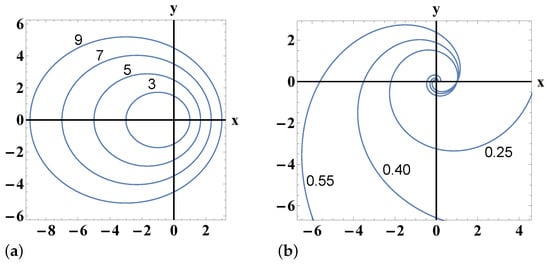
We consider the monoparametric family of orbits (ellipses, see Figure 1a)

$$f(x,y)=x+2\sqrt{x^2+y^2}=c,$$

(20)

which leads to the slope function

$$\gamma =\frac{2y}{2x+\sqrt{x^2+y^2}},\Gamma \ne 0,$$

(21)

Here, we have $q_2,q_1\ne$ 0, and we check the condition (18). It is satisfied, and we determine the function $\mathcal{Q}\left(u\right)$ from (15). It is:

$$\mathcal{Q}\left(u\right)=-\frac{3}{2u},u=x^2+y^2,$$

(22)

and, from (19), we find

$$\mathcal{P}\left(u\right)=-\frac{2d_1}{\sqrt{u}}+d_2,d_1,d_2=const.$$

(23)

If we set $d_1=\frac{1}{2}$ and $d_2=$ 0, we conclude that the family of orbits (20) is created by the Newtonian potential

$$V(x,y)=-\frac{1}{\sqrt{x^2+y^2}}.$$

(24)

The potential in (24) is non-integrable ([19]). The polynomial integrability of two-dimensional Hamiltonian systems with homogeneous potentials of degree $-k$ was also studied by [20]. The energy of the family of orbits (20) is found from (7) to be

$$\mathcal{E}=-\frac{3}{4c}=const.$$

(25)

and the allowed region is found from (8) to be $A=x+2\sqrt{x^2+y^2}\ge$0.

Figure 1. (a) Some members of the family of orbits (20) (ellipses) for $c=$ 3, 5, 7, 9. (b) Members of the family of orbits (26) for $a=$ 1 and $b=$ 0.25, 0.4, and 0.55 successively.

Example 2.

We regard the curves (logarithmic spirals, see Figure 1b) in the 2D Euclidean plane

$$x=a{e}^{bt}cost,y=a{e}^{bt}sint,a,b\ne 0.$$

(26)

Eliminating the parameter t from the Equation (26), we obtain the monoparametric family of orbits in $x,y$-coordinates

$$f(x,y)=(x^2+y^2)exp\left(-2barctan\left(\frac{y}{x}\right)\right)=a^2=c,$$

(27)

which is represented by the slope function

$$\gamma =\frac{-bx+y}{x+by},\Gamma \ne 0,$$

(28)

Here, it is $q_2,q_1\ne$ 0, and we check the condition (18). It is satisfied, and we determine the function $\mathcal{Q}\left(u\right)$ from (15). It is:

$$\mathcal{Q}\left(u\right)=-\frac{2}{u},u=x^2+y^2,$$

(29)

and, from (19), we find

$$\mathcal{P}\left(u\right)=-\frac{d_1}{u}+d_2,d_1,d_2=const.$$

(30)

If we set $d_1=1$ and $d_2=$ 0, we conclude that the family of orbits (27) is produced by the potential (homogeneous of degree $m=-$2)

$$V(x,y)=-\frac{1}{x^2+y^2}.$$

(31)

The potential in (31) is completely integrable as it was shown by ([20], p. 3878). The energy is found to be (7)

$$\mathcal{E}=0.$$

(32)

and the allowed region is the entire plane. We note here that the family of orbits (27) is trcaced isoenergetically ($\mathcal{E}$ = 0) by a material point of unit mass under the action of potential (31). Such families of planar orbits were studied in detail by [15].

Special Cases

In this paragraph, we shall present one example that corresponds to the Case 2 of the general theory.

Example 3.

We take into account the monoparametric family of orbits (circles)

$$f(x,y)=x^2+y^2=c,$$

(33)

which leads to the slope function

$$\gamma =\frac{y}{x},\Gamma =-\frac{x^2+y^2}{x^3}\ne 0.$$

(34)

Here, we have $q_2=q_1=$ 0 (Case 2). Thus, any function $V=\mathcal{P}\left(u\right)$ is a solution to our problem. Thus, we have

$$\mathcal{P}\left(u\right)=\mathcal{R}\left(u\right),$$

(35)

where $\mathcal{R}$ is an arbitrary function of $C^2$−class. The corresponding potential is

$$V(x,y)=\mathcal{R}(x^2+y^2).$$

(36)

It is remarkable to say that

a. 

If we select $R\left(u\right)=\sqrt{1+u}$, then we obtain the cored potential $V=\sqrt{1+x^2+y^2}$, and the energy of the family of orbits is

$$\mathcal{E}=\frac{2+3c}{2\sqrt{1+c}}$$

and the allowed region is the entire plane ($A=-\frac{x^2}{\sqrt{1+x^2+y^2}}\le$ 0).

b. 

If we select $R\left(u\right)=log(1+u)$, then we obtain the loagarithmic potential $V=log(1+x^2+y^2)$ and the energy of the family of orbits is

$$\mathcal{E}=\frac{c}{1+c}+log(1+c)$$

and the allowed region is the entire plane ($A=-\frac{2x^2}{1+x^2+y^2}\le$ 0).

Both of them were studied in [21].

5. Potentials of the Form $\mathcal{P}=\mathcal{P}\left(xy\right)$

At the beginning, we shall prove the following

Theorem 1.

All of the monoparametric families of orbits $f(x,y)=\mathcal{M}(x^2+y^2)=c$ where $\mathcal{M}$ is an arbitrary function of $C^2-$class are produced by the potential $V(x,y)=-\frac{1}{xy}$ and the allowed region for a test particle is $xy>$ 0 ($A=-\frac{2x}{y(x^2+y^2)}\le$ 0).

Proof. 

We consider the family of orbits

$$f(x,y)=\mathcal{M}(x^2+y^2)=c,$$

(37)

where $\mathcal{M}$ is an arbitrary function of $C^2-$class and the slope function is

$$\gamma =\frac{y}{x},\Gamma \ne 0.$$

(38)

Here, it is $q_2,q_1\ne$ 0, and we check the condition (18). It is satisfied, and we determine the function $\mathcal{Q}\left(u\right)$ from (15). It is:

$$\mathcal{Q}\left(u\right)=-\frac{2}{u},u=xy,$$

(39)

and, from (19), we find

$$\mathcal{P}\left(u\right)=-\frac{d_1}{u}+d_2,d_1,d_2=const.$$

(40)

For $d_1=1$, $d_2=$ 0, the potential function is

$$V(x,y)=-\frac{1}{xy}.$$

(41)

which is non-integrable in Liouville sense ([22], p. 80). Proceeding more, we present the following. □

Example 4.

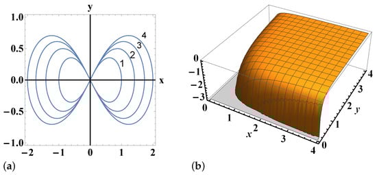
We consider the curves (lemniscates of Bernoulli) on the 2D plane (see Figure 2a)

$$x^2+y^2=2a^2(x^2-y^2),a\ne 0.$$

(42)

This family of curves can be written as follows:

$$f(x,y)=\frac{x^2+y^2}{x^2-y^2}=2a^2=c,$$

(43)

which is related to the slope function

$$\gamma =\frac{3x^{2}y-y^3}{x^3-3x{y}^2},\Gamma \ne 0.$$

(44)

Here, it is $q_2,q_1\ne$ 0, and we check the condition (18). It is satisfied, and we determine the function $\mathcal{Q}\left(u\right)$ from (15). It is:

$$\mathcal{Q}\left(u\right)=-\frac{5}{2u},u=xy,$$

(45)

and, from (19), we find

$$\mathcal{P}\left(u\right)=-\frac{2d_1}{3u^{3/2}}+d_2,d_1,d_2=const.$$

(46)

For $d_1=1$ and $d_2=$ 0, the potential function is

$$V(x,y)=-\frac{2}{3{\left(xy\right)}^{3/2}},$$

(47)

The potential in (47) is integrable in the Liouville sense ([22], p. 80), and the energy of the family of orbits (43) is found to be $\mathcal{E}$ = 0. The allowed region for a test particle is $xy>$ 0 ($A=-\frac{4{(x^3-3x{y}^2)}^2}{3{\left(xy\right)}^{3/2}{(x^2+y^2)}^3}\le$ 0).

Figure 2. (a) Some members of the family of orbits (43) for $c=$ 1, 2, 3, and 4. (b) A 3D plot of the potential (47), which produces the family of orbits (42).

Other results are presented at Table 1.

Table 1. Families of orbits and potentials.

Family of Orbits	Potential V(x,y)	Energy	Allowed Region
$f(x,y)=x^{4/3}+y^{4/3}=c$	$-\frac{3}{2{\left(xy\right)}^{2/3}}$	$\frac{3}{c}$	y > 0
$f(x,y)=xy(x+y)=c$	$\frac{d_1}{6}{x}^6{y}^6$ ($d_1<$0)	$-\frac{1}{12}{d}_1{c}^4$	the entire plane

The first potential is integrable in Liouville sense ([22], p. 81), but the second one is non-integrable.

Special Cases

In this paragraph, we shall present two examples that correspond to the Cases 1 and 3 of the general theory.

Example 5.

As we explained in Section 2, a monoparametric family of orbits $f(x,y)=c$ can be represented by the slope function γ. Thus, here we shall consider a family of orbits studied by ([6], p. 470) that corresponds to

$$\gamma =-r+s,$$

(48)

where

$$r=\frac{2xy-1}{x^2+y^2},s=\sqrt{r^2-1}$$

(49)

Here, we have $q_2\ne 0,q_1=$ 0 (Case 1), and we check the condition (18). It is satisfied, and we find the function $\mathcal{Q}\left(u\right)$ from (15). It is: $\mathcal{Q}\left(u\right)$ = 0, and the function $\mathcal{P}=\mathcal{P}\left(u\right)$ is found to be

$$\mathcal{P}\left(u\right)=d_{1}u+d_2,d_1,d_2=const.$$

(50)

If we set $d_1=1$ and $d_2=$ 0, we find the two-dimensional potential

$$V(x,y)=xy.$$

(51)

The potential in (51) is non-integrable ([20,22]), and the energy of this family of orbits is $\mathcal{E}=\frac{1}{2}$.

Example 6.(Counterexample)

We take into account the monoparametric family of orbits

$$f(x,y)=xy(1+xy)=c,$$

(52)

which leads to the slope function

$$\gamma =\frac{x}{y},\Gamma =\frac{2x}{y^2}\ne 0,$$

(53)

Here, we have $q_2=0,q_1\ne$ 0 (Case 3). Thus, $\mathcal{P}\left(u\right)=const.$, which is excluded from our study. So, there is no solution to our problem.

6. Cubic Potentials

In this Section, we shall deal with polynomial potentials of degree $m=$ 3. We select $u=x^3+k{y}^3$ ($k\in \mathbb{Z},k\ne 0$), and we start with

Example 7.

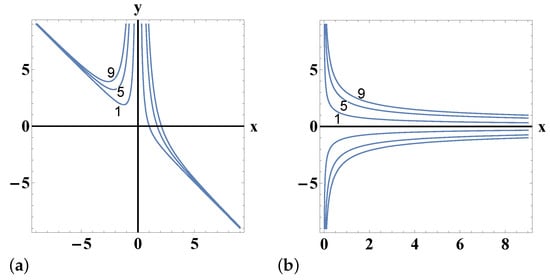
We shall examine the family of orbits (see Figure 3a)

$$f(x,y)=x^3+x^{2}y=c,c=const.$$

(54)

which leads to the slope function

$$\gamma =\frac{x}{3x+2y},\Gamma \ne 0,$$

(55)

and we shall search the potentials of the form

$$V(x,y)=\mathcal{P}\left(u\right),u=x^3+k{y}^3,k=const.$$

(56)

We check the condition (18). It is satisfied only for $k=-$1, and this leads to the case $q_2\ne 0,q_1=$ 0 (Case 1). Then, we determine the function $\mathcal{Q}\left(u\right)$. It is as follows: $\mathcal{Q}\left(u\right)$ = 0 and the potential function is given by

$$\mathcal{P}\left(u\right)=d_{1}u+d_2,d_1,d_2=const.$$

(57)

For $d_1=1$ and $d_2$ = 0, we obtain

$$V(x,y)=x^3-y^3.$$

(58)

This result agrees with the result found by ([6], p. 471) by using another methodology. We note here that the potential in (58) is separable in Cartesian coordinates and, consequently, is integrable ([19], pp. 8614, 8619). The energy of the family of orbits is calculated from (7)

$$\mathcal{E}=-\frac{13}{2}c=const.$$

(59)

and the allowed region for a test particle is $3x-y\le$ 0 ($A=\frac{1}{2}(3x-y){(3x+2y)}^2\le$ 0).

Figure 3. (a) Some members of the family of orbits (54) for c = 1, 5, and 9. (b) Some members of the family of orbits (60) for c = 1, 5, 9, and m = 2.

Some interesting results are shown at Table 2 ($d_1,d_2>0$).

Table 2. Families of orbits and potentials.

Family of Orbits	Potential V(x,y)	Energy	Allowed Region
$f(x,y)=x{(x+y)}^2=c$	$d_{2}y(3x^2+y^2)$	$-\frac{13d_2}{2}c$	$x+2y$ < 0
$f(x,y)=y{(x+y)}^2=c$	$d_{1}x(x^2+3y^2)$	$-\frac{13d_1}{2}c$	$2x+y$ < 0

7. Other Results

Potentials of the Form $V=\mathcal{P}\left(\frac{x}{y}\right)$

We shall prove the following

Theorem 2.

All the monoparametric families of orbits $f(x,y)=f(x,y)=x{y}^m=c$ ($m\ne 0,-1$) are produced by the potential $V(x,y)=-\frac{y^2}{2m(m{x}^2-y^2)}$.

Proof. 

We regard the family of orbits

$$f(x,y)=x{y}^m=c,m\ne 0,-1,$$

(60)

which leads to the slope function

$$\gamma =\frac{mx}{y},\Gamma =\frac{m(m+1)x}{y},$$

(61)

and we shall look for potentials of the form

$$V(x,y)=\mathcal{P}\left(u\right),u=x{y}^n,n\ne m.$$

(62)

We check the condition (18). It is satisfied only for $n=-$1. Thus, we take $u=\frac{x}{y}$, and we are interested in potentials

$$V(x,y)=\mathcal{P}\left(\frac{x}{y}\right).$$

(63)

The fact $n=-$1 leads to the case $q_2,q_1\ne 0$. Then, we determine the function $\mathcal{Q}\left(u\right)$. It is:

$$\mathcal{Q}\left(u\right)=\frac{1+3m{u}^2}{u-m{u}^3},$$

(64)

and the potential function is given by

$$\mathcal{P}\left(u\right)=\frac{d_1}{2m(1-m{u}^2)}+d_2,d_1,d_2=const.$$

(65)

For $d_1=1$ and $d_2$ = 0, we obtain

$$V(x,y)=-\frac{y^2}{2m(m{x}^2-y^2)},$$

(66)

which is homogeneous of zero degree. The energy of the family of orbits is

$$\mathcal{E}=\frac{1}{2(1+m)}=const.$$

(67)

and the allowed region for a test particle is determined from (8). It is:

$$A=-\frac{y^2}{m(m+1)(m{x}^2-y^2)}\le 0.$$

(68)

From (68), we conclude that the area for the motion of test particle is $A=m{x}^2-y^2>$ 0 for $m>$ 0, or, for $m<$ 0. In the next step, we offer the following. □

Example 8.

We consider the monoparametric family of orbits (astroids curves, see Figure 4a)

$$f(x,y)=x^{2/3}+y^{2/3}=c,$$

(69)

which leads to the slope function

$$\gamma =\frac{x^{1/3}}{y^{1/3}},\Gamma \ne 0,u=\gamma .$$

(70)

From (15) we obtain $q_2,q_1\ne$ 0, and we check the condition (18). It is satisfied, and we determine the function $\mathcal{Q}\left(u\right)$ from (15). It is:

$$\mathcal{Q}\left(u\right)=-\frac{1+2u^2+3u^4}{u(u^4-1)},$$

(71)

and, from (19), we find

$$\mathcal{P}\left(u\right)=\frac{d_1\sqrt{1-u^4}}{2(1-u^2)}+d_2,d_1,d_2=const.$$

(72)

and the allowed region is $A=y^{2/3}-x^{2/3}>$ 0.

Figure 4. (a) Some members of the family of orbits (69) for c = 0.04, 0.36, and 1. (b) Some members of the family of orbits (80) for c = 0.25, 0.5, and 1.

8. Integrable Potentials

A Hamiltonian system with n degrees of freedom is integrable if the system admits n independent first integrals in involution (Liouville integrability). Let us consider a two-degree of freedom Hamiltonian

$$H=\frac{1}{2}(p_x^2+p_y^2)+V(x,y).$$

(73)

We assume that $\Phi$ is a first integral of (73). Then, the Poisson bracket of $\Phi$ and H vanishes, i.e.,

$$[\Phi ,H]=0.$$

The question of integrability of 2D potentials was addressed by many authors in the past. More precisely, Ref. [23] studied a family of dynamical systems related to the motion of a test particle in two-dimensional space and found integrals of motion quadratic in velocities. The same authors extended their work to third- and fourth degree-polynomial potentials ([24]). In both cases, they used the weak-Pianlevé property as a criterion for integrability. Polynomial integrals of motion of a degree greater than 2 for planar systems have been found in the review paper of [25]. Integrable velocity-dependent potentials that have linear or quadratric invariants in the velocity have been studied by [26]; integrable velocity-dependent potentials with logarithmic integrals of motion were found by [27]. In [28], the author derived a new equation equivalent to the equation that follows from the condition of vanishing Poisson bracket for autonomous systems of two degrees of freedom. In addition to that, Ref. [29] formulated four necessary and sufficient conditions for a potential function $U(x,y)$ in order to be integrable with the second integral of motion quartic in velocities. In the meanwhile, Ref. [30] combined the results of Darboux’s theory with the inverse problem of dynamics and found monoparametric families of orbits sufficient for the integrability of planar potentials having linear or quadratic invariants. Proceeding further, Ref. [31] found planar potentials with a second integral quadratic in the momenta by using Darboux’s integrability criterion. Ref. [19] gave a complete list of all of the integrable two-dimensional homogeneous polynomial potentials with a polynomial integral of order of at most four in the momenta. For algebraic homogeneous potentials of a non-zero rational homogeneity degree, necessary integrability conditions were constructed by [22]. The polynomial integrability of Hamiltonian systems with homogeneous potentials of degree $-k$ was examined by [20].

As an example, we shall study an integrable potential (see [19], p. 8614), a polynomial of the third degree, and we shall find a family of planar orbits compatible with it. This is

$$V(x,y)=x^3+\frac{3}{16}x{y}^2.$$

(74)

Example 9.

We shall consider the family of orbits

$$f(x,y)=f(x,y)=f(x,y)=x{y}^m=c,m\ne 0,-1,$$

(75)

which leads to the slope function

$$\gamma =\frac{mx}{y},\Gamma \ne 0,$$

(76)

and we shall search potentials of the form

$$V(x,y)=\mathcal{P}\left(u\right),u=x^3+\frac{3}{16}x{y}^2.$$

(77)

We check the condition (18). It is satisfied only for $m=-$4, and this leads to the case $q_2\ne 0,q_1$ = 0 (Case 1). Then, we determine the function $\mathcal{Q}\left(u\right)$. It is: $\mathcal{Q}\left(u\right)$ = 0, and the potential function is given by

$$\mathcal{P}\left(u\right)=d_{1}u+d_2,d_1,d_2=const.$$

(78)

For $d_1=1$ and $d_2$ = 0, we find the potential

$$V(x,y)=x^3+\frac{3}{16}x{y}^2.$$

(79)

which produces the family of orbits

$$f(x,y)=\frac{x}{y^4}=c.$$

(80)

and the allowed region is $x<$ 0 ($A=\frac{8x^2{y}^2+y^4}{64x}\le$ 0).

9. One-Dimensional Potentials

In this Section, we shall examine potentials of the form $V=V\left(y\right)$.

Example 10.

We consider the monoparametric family of orbits (parabolas)

$$f(x,y)=x+y^2=c,$$

(81)

which is represented by the slope function

$$\gamma =2y,\Gamma =-2\ne 0,$$

(82)

and we shall find potentials of the form

$$V(x,y)=\mathcal{P}\left(u\right),u=\gamma .$$

(83)

From (14), we find the quantities $q_1,q_2$. These are: $q_1=-\frac{6}{y},q_2=4$, and $\mathcal{Q}\left(y\right)=-\frac{3}{2y}$. The condition (18) is satisfied, and thus we have $\mathcal{Q}\left(u\right)=-\frac{3}{u}$. From (19), we determine the potential function $\mathcal{P}=\mathcal{P}\left(u\right)$.

$$\mathcal{P}=-\frac{d_1}{2u^2}+d_2,d_1,d_2\ne 0.$$

(84)

If we set $d_1=1$ and $d_2=$ 0, then we obtain

$$V(x,y)=-\frac{1}{8y^2}.$$

(85)

The potential (85) is integrable, and it was studied in detail by ([31], p. 1635). The energy of the family of orbits (81) is $\mathcal{E}=\frac{1}{2}$ and the allowed region is the entire plane ($A=-\frac{1}{8y^2}\le$ 0).

10. Families of Straight Lines

If $\Gamma$ = 0, then we have to study a one-parameter family of straight lines (FSL) in 2-D space. As it was shown by [14], potentials that generate one-parametric families of straight lines on the $xy-$plane have to satisfy the following necessary and sufficient differential condition:

$$\begin{array}{c}\hfill V_x{V}_y(V_{xx}-V_{yy})=V_{xy}(V_x^2-V_y^2).\end{array}$$

(86)

We examined the following potentials:

I.

$V=\mathcal{P}(x^2+y^2)$,

II.

$V=\mathcal{P}(c_{1}x+c_{2}y)$, $c_1,c_2=const.$

III.

$V=\mathcal{P}\left(x{y}^n\right)$, $n\ne$ 0

IV.

$V=\mathcal{P}(x^3+k{y}^3)$, $k\ne$ 0

We replaced them into (86), and we found that only the first two cases, i.e., I and II, are applicable for the study of straight lines. Then, we find the corresponding family of staight lines

$$\gamma =-\frac{V_x}{V_y}.$$

(87)

For the first case, we obtain

$$\gamma =-\frac{x}{y}$$

(88)

and the family of straight lines is

$$f(x,y)=\frac{y}{x}=c.$$

(89)

For the second case, we obtain

$$\gamma =-\frac{c_1}{c_2}=c_3,$$

(90)

or, equivalently,

$$f(x,y)=y=c_{3}x+c_4,c_3,c_4=const.$$

(91)

11. Conclusions

In the present paper, we studied four solvable versions of the 2D inverse problem of Newtonian dynamics, and we gave the reader a new idea on how to find new solutions to it by using the basic equations. This problem relates two-dimensional potentials $V=V(x,y)$ with a preassigned monoparametric family of regular orbits $f(x,y)=c$ = const.

We used the basic PDE (6) of the inverse problem of dynamics, taking into account that the quantity $\Gamma$ is different from zero (Section 2). We imposed one differential condition on the slope function $\gamma$, i.e., Equation (18), in order to have solutions for our problem. We studied potentials of the form $V(x,y)=\mathcal{P}\left(u\right)$ where $u=x^2+y^2,xy,x^3-y^3,\frac{x}{y}$ ($x,y\ne$ 0). We focused our interest on central potentials that have many applications in physical problems. In order to obtain interesting results, we studied known curves in the $xy-$plane, e.g., circles, ellipses, logarithmic spirals, lemniscates of Bernoulli, etc., which can be traced by a test particle of unit mass as orbits. Our results were not restricted only to central potentials, but we extended them to homogeneous potentials of degree m and to other known potentials from the bibliography, i.e., cubic potentials. We did not obtain only mathematical results; we also found potentials with applications in many areas of physics, e.g., galactic dynamics. Such potentials are the following ones: the Newtonian, the cored, and the logarithmic ones. Our aim was to find a suitable pair of orbits that are produced by these potentials. Furthermore, we found monoparametric families of orbits produced by integrable potentials. New figures with families of orbits were presented in all cases. All of the results are really new and original. We also studied the case of straight lines, which is a special category of orbits in 2D space.

References

- Szebehely, V. On the determination of the potential by satellite observations. In Proceedings of the International Meeting on Earth’s Rotation by Satellite Observation; Proverbio, G., Ed.; The University of Cagliari: Bologna, Italy, 1974; pp. 31–35. [Google Scholar]
- Bozis, G. Generalization of Szebehely’s Equation. Cel. Mech. 1983, 29, 329–334. [Google Scholar] [CrossRef]
- Bozis, G.; Tsarouhas, G. Conservative fields derived from two monoparametric families of planar orbits. Astron. Astrophys. 1985, 145, 215–220. [Google Scholar]
- Puel, F. Intrinsic formulation of the equation of Szebehely. Cel. Mech. 1984, 32, 209–216. [Google Scholar] [CrossRef]
- Bozis, G. Szebehely’s inverse problem for finite symmetrical material concentrations. Astron. Astrophys. 1984, 134, 360–364. [Google Scholar]
- Bozis, G.; Grigoriadou, S. Families of planar orbits generated by homogeneous potentials. Cel. Mech. Dyn. Astr. 1993, 57, 461–472. [Google Scholar] [CrossRef]
- Bozis, G.; Anisiu, M.-C.; Blaga, C. Inhomogeneous potentials producing homogeneous orbits. Astron. Nach. 1997, 318, 313–318. [Google Scholar] [CrossRef]
- Bozis, G.; Ichtiaroglou, S. Boundary Curves for Families of Planar Orbits. Cel. Mech. Dyn. Astr. 1993, 58, 371–385. [Google Scholar] [CrossRef]
- Bozis, G. The inverse problem of dynamics: Basic facts. Inverse Probl. 1995, 11, 687–708. [Google Scholar] [CrossRef]
- Grigoriadou, S.; Bozis, G.; Elmabsout, B. Solvable cases of Szebehely’s equation. Cel. Mech. Dyn. Astr. 1999, 74, 211–221. [Google Scholar] [CrossRef]
- Anisiu, M.-C.; Bozis, G.; Blaga, C. Special families of orbits in the direct problem of dynamics. Cel. Mech. Dyn. Astr. 2004, 88, 245–257. [Google Scholar] [CrossRef]
- Blaga, C.; Anisiu, M.-C.; Bozis, G. New solutions in the direct problem of dynamics. PADEU 2006, 17, 13. [Google Scholar]
- Bozis, G.; Anisiu, M.-C.; Blaga, C. A solavable version of the direct problem of dynamics. Rom. Astron. J. 2000, 10, 59–70. [Google Scholar]
- Bozis, G.; Anisiu, M.-C. Families of straight lines in planar potentials. Rom. Astron. J. 2001, 11, 27–43. [Google Scholar]
- Borghero, F.; Bozis, G. Isoenergetic families of planar orbits generated by homogeneous potentials. Meccanica 2002, 37, 545–554. [Google Scholar] [CrossRef]
- Anisiu, M.-C. An alternative point of view on the equations of the inverse problem of dynamics. Inverse Probl. 2004, 20, 1865–1872. [Google Scholar] [CrossRef]
- Bozis, G.; Anisiu, M.-C. A solvable version of the inverse problem of dynamics. Inverse Probl. 2005, 21, 487–497. [Google Scholar] [CrossRef]
- Bozis, G.; Meletlidou, E. Nonintegrability Detected from Geometrically Similar Orbits. Cel. Mech. Dyn. Astr. 1997, 68, 335–346. [Google Scholar] [CrossRef]
- Nakagawa, K.; Yoshida, H. A list of all integrable two-dimensional homogeneous polynomial potentials with a polynomial integral of order at most four in the momenta. J. Phys. A Math. Gen 2001, 34, 8611–8630. [Google Scholar] [CrossRef]
- Oliveira, R.; Valls, C. Polynomial integrability of Hamiltonian systems with homogeneous potentials of degree -k. Phys. Let. A 2016, 380, 3876–3880. [Google Scholar] [CrossRef]
- Jimenez-Lara, L.; Llibre, J. The cored and logarithmic potentials: Periodic orbits and integrability. J. Math. Phys. 2012, 53, 1–12. [Google Scholar] [CrossRef]
- Maciejewski, A.; Przybylska, M. Integrability of Hamiltonian systems with algebraic potentials. Phys. Let. A 2016, 380, 76–82. [Google Scholar] [CrossRef]
- Dorizzi, B.; Grammaticos, B.; Ramani, A. A new class of integrable systems. J. Math. Phys. 1983, 24, 2282–2288. [Google Scholar] [CrossRef]
- Dorizzi, B.; Grammaticos, B.; Ramani, A. Integrability of Hamiltonians with third- and fourth-degree polynomial potentials. J. Math. Phys. 1983, 24, 2288–2295. [Google Scholar]
- Hietarinta, J. Direct methods for the search of second invariants. Phys. Rep. 1987, 147, 87–154. [Google Scholar] [CrossRef]
- Dorizzi, B.; Grammaticos, B.; Ramani, A. Integrable Hamiltonian systems with velocity-dependent potentials. J. Math. Phys. 1985, 26, 3070–3079. [Google Scholar] [CrossRef]
- Icthiaroglou, S.; Voyatzis, G. Integrable potentials with logarithmic integrals of motion. J. Phys. A Math. Gen. 1988, 21, 3537–3546. [Google Scholar] [CrossRef]
- Bozis, G. A transformed equation for a vanishing Poisson bracket. J. Phys. A Math. Gen. 1989, 22, 1759–1764. [Google Scholar] [CrossRef]
- Bozis, G. Two-dimensional integrable potentials with quartic invariants. J. Phys. A Math. Gen. 1992, 25, 3329–3351. [Google Scholar] [CrossRef]
- Icthiaroglou, S.; Meletlidou, E. On monoparametric families of orbits sufficient for integrability of planar potentials with linear or quadratic invariants. J. Phys. A Math. Gen. 1990, 23, 3673–3679. [Google Scholar] [CrossRef]
- Grigoriadou, S. The inverse problem of dynamics and Darboux’s integrability criterion. Inverse Probl. 1999, 15, 1621–1637. [Google Scholar] [CrossRef]
Disclaimer/Publisher’s Note: The statements, opinions and data contained in all publications are solely those of the individual author(s) and contributor(s) and not of MDPI and/or the editor(s). MDPI and/or the editor(s) disclaim responsibility for any injury to people or property resulting from any ideas, methods, instructions or products referred to in the content. |
© 2023 by the author. Licensee MDPI, Basel, Switzerland. This article is an open access article distributed under the terms and conditions of the Creative Commons Attribution (CC BY) license (https://creativecommons.org/licenses/by/4.0/).