On Perfectness of Systems of Weights Satisfying Pearson’s Equation with Nonstandard Parameters

Abstract

Measures generating classical orthogonal polynomials are determined by Pearson’s equation, whose parameters usually provide the positivity of the measures. The case of general complex parameters (nonstandard) is also of interest; the non-Hermitian orthogonality with respect to (now complex-valued) measures is considered on curves in $\mathbb{C}$. Some applications lead to multiple orthogonality with respect to a number of such measures. For a system of r orthogonality measures, the perfectness is an important property: in particular, it implies the uniqueness for the whole family of corresponding multiple orthogonal polynomials and the $(r+2)$-term recurrence relations. In this paper, we introduce a unified approach which allows to prove the perfectness of the systems of complex measures satisfying Pearson’s equation with nonstandard parameters. We also study the polynomials satisfying multiple orthogonality relations with respect to a system of discrete measures. The well-studied families of multiple Charlier, Krawtchouk, Meixner and Hahn polynomials correspond to the systems of measures defined by the difference Pearson’s equation with standard real parameters. Using the same approach, we verify the perfectness of such systems for general parameters. For some values of the parameters, discrete measures should be replaced with the continuous measures with non-real supports.

1. Introduction

Let $\mathbb{C}\left[z\right]$ be the linear space of polynomials with complex coefficients, and let there be $r\in {\mathbb{Z}}_{>0}$ linear functionals $l_j:\mathbb{C}\left[z\right]\to \mathbb{C}$, $j=1,\dots ,r$. Each of the functionals $l_j$ may be defined by a sequence of its moments $s_{j,k}:=l_j\left(z^{k-1}\right)$, $k\in {\mathbb{Z}}_{>0}$.

Given a (multi-)index $\mathit{n}=(n_1,\dots ,n_r)\in {\mathbb{Z}}_{⩾0}^r$, a non-trivial polynomial $P_{\mathit{n}}\in \mathbb{C}\left[z\right]$ of degree at most

$$\left|\mathit{n}\right|:=n_1+\dots +n_r$$

is called a (type II) multiple orthogonal polynomial if it satisfies the following orthogonality conditions:

$$l_j\left(P_{\mathit{n}}\left(z\right)z^k\right)=0,k=0,\dots ,n_j-1,j=1,\dots ,r.$$

(1)

These orthogonality conditions reduce to a homogeneous linear algebraic system for the coefficients of $P_{\mathit{n}}$, which always has a nontrivial solution.

The polynomials $P_{\mathit{n}}$ play the role of denominators of the Hermite–Padé approximants $\frac{Q_{\mathit{n},j}}{P_{\mathit{n}}}$ for a set of formal power series $f_j\left(z\right):={\sum }_{k=1}^{\infty }\frac{s_{j,k}}{z^k}$. That is, the following interpolation conditions at infinity are satisfied:

$$(P_{\mathit{n}}{f}_j-Q_{\mathit{n},j})\left(z\right)=O\left(z^{-n_j-1}\right)\mathrm{as}z\to \infty ,j=1,\dots ,r.$$

(2)

It is an easy exercise to show that the orthogonality conditions (1) are equivalent to the interpolation conditions (2). The corresponding numerators $Q_{\mathit{n},j}$ can be defined as the polynomial parts of power series expansions of $P_{\mathit{n}}{f}_j$ at infinity.

On applying a construction of this kind, C. Hermite proved [1] that the number e is transcendental. Some modern applications of multiple orthogonality to number theory can be found in reviews [2,3] and papers [4,5]. Other important applications include random matrices [6], spectral theory [7] and integrable systems [8].

Definition 1. 

The index $\mathit{n}$ is called normal, if any non-trivial polynomial $P_{\mathit{n}}$ satisfying $deg{P}_{\mathit{n}}⩽\left|\mathit{n}\right|$ and (1) has $deg{P}_{\mathit{n}}=\left|\mathit{n}\right|$.

Normality implies the uniqueness of the rational Hermite–Padé approximants, as well as the uniqueness of the multiple orthogonal polynomials up to multiplication by a nonzero constant.

Definition 2. 

The system of functionals $l_j$ is called perfect if all its indices $\mathit{n}\in {\mathbb{Z}}_{⩾0}^r$ are normal.

The definition of perfect systems was given by K. Mahler in [9]. In the case $r=1$, the above notions reduce to ordinary orthogonal polynomials with respect to a functional and to the Padé approximants. For $r=1$, the notion of perfectness reduces to the so-called quasi-definiteness of the functional; see ([10], p. 16).

Consider the particular case of functionals determined by positive continuous weights $w_j$ on an interval E of the real line:

$$l_j\left(Q\right)={\int }_{E}Q\left(x\right)w_j\left(x\right)dx,Q\in \mathbb{C}\left[x\right].$$

The system of weights $w_j$ is called an AT system if for each $\mathit{n}\in {\mathbb{Z}}_{⩾0}^r$ any nontrivial linear combination with polynomial coefficients

$$\sum _{j=1}^r{A}_j{w}_j,A_j\in \mathbb{R}\left[x\right],\mathrm{deg}{A}_j<n_j,\sum _{j=1}^r{A}_j^2\not\equiv 0,$$

has at most $\left|\mathit{n}\right|-1$ zeros on E. It is not hard to show [11], that AT-systems are perfect, i.e., that the corresponding systems of linear functionals are perfect. Moreover, the corresponding polynomials $P_{\mathit{n}}$ have $\left|\mathit{n}\right|$ simple zeros in E. These properties are helpful for constructing generalized Gaussian quadratures; see [12,13,14].

Among special functions, an important role is played by classical orthogonal polynomials. They can be written in terms of hypergeometric functions; they admit explicit representations through Rodrigues’s formula and so on. Classification (see [15]) of such polynomials for $r=1$ can rely on differential Pearson’s equation for the orthogonality weight

$${\left(\sigma w\right)}^{\prime }=\tau w,$$

(3)

where $\sigma$ and $\tau$ are polynomials such that $deg\sigma ⩽2$ and $deg\tau ⩽1$. In this way, one obtains classical polynomials named after Hermite, Laguerre and Jacobi; one also obtains the Bessel polynomials orthogonal with respect to a complex measure on a complex curve.

It is also of interest to consider a system of classical weights $w_j$ satisfying Pearson’s equation with the common $\sigma$, but distinct ${\tau }_j$. For standard restrictions on coefficients of $\sigma$ and ${\tau }_j$, this is also an AT-system, and the corresponding orthogonal polynomials admit explicit expressions via Rodrigues’s formula. Such systems are classified in [16,17].

Multiple orthogonal polynomials constructed in this manner turn to be closely related to certain problems from the theory of random matrices. In particular, the multiple Hermite polynomials account for probabilistic characteristics of non-intersecting Brownian bridges [18] and eigenvalues of Gaussian unitary ensembles with an external source [19]. The multiple Laguerre polynomials lead to the so-called Wishart ensembles [20]. These polynomials together with the Jacobi–Piñeiro polynomials [21] (i.e., the multiple Jacobi polynomials) are related to interesting problems in percolation theory [22].

Classical weights with nonstandard parameters are also of interest. In this case, the orthogonality with respect to complex measures $w_j\left(z\right)dz$ is considered [23] on complex curves. For $r=1$, the questions of uniqueness and of the asymptotic behavior of classical orthogonal polynomials with nonstandard parameters were studied in works [24,25,26]. For $r>1$, the Jacobi–Piñeiro polynomials with nonstandard parameters allowed to construct a counterexample to the Gaudin Bethe Ansatz conjecture; see [27].

In this work, we study the perfectness of systems of weights satisfying differential Pearson’s equation with nonstandard parameters. Note that an analogous question for the multiple Wilson and Jacobi–Piñeiro polynomials was considered in the remarkable paper [28]. Our approach may be seen as a development of the approach of [28]: we rely on raising operators, which allows us to treat the case of difference Pearson’s equations in a similar manner.

On replacing the differential Pearson’s equation with its difference analogue

$$\left(\sigma w\right)(x+1)-\left(\sigma w\right)\left(x\right)=\left(\tau w\right)\left(x\right),$$

(4)

one arrives at the classification of classical polynomials orthogonal with respect to discrete measures: the Charlier, Meixner, Hahn and Krawtchouk polynomials. These families of polynomials were treated in detail in monograph [29]. Moreover, it is known that, for instance, the Meixner polynomials for some nonstandard values of parameters turn into the Meixner–Pollaczek polynomials whose orthogonality weight is continuous; see [30]. An analogous connection exists [31] between discrete and continuous Hahn polynomials. We revisit this phenomenon in Section 5. Modern applications of discrete orthogonal polynomials may be found in ref. [32].

The classification of discrete multiple orthogonal polynomials (the case $r>1$) based upon difference Pearson’s Equation (4) was made in the striking paper [33]. A relation of multiple Charlier polynomials to representations of the Heisenberg–Weyl algebra was found in [34]. There is an expression of the Hermite–Padé approximants for the remainder terms of power series of exponential functions via the multiple Charlier polynomials with nonstandard parameters; see [35]. The multiple Meixner polynomials arise in the description of non-Hermitian oscillator Hamiltonians [36,37]. Applications of the multiple Meixner–Pollaczek polynomials to the six-vertex model were studied in [38]. By applying our unified approach to normality and perfectness, we give a detailed answer for which values of the parameters, the systems of weights defined by difference Pearson’s equation, are perfect.

In ([39], Theorem 23.1.11) (see also [40]), W. Van Assche proved that multiple orthogonal polynomials induced by perfect systems satisfy the so-called nearest-neighbor recurrence relations on the lattice of indices. This leads to applications in discrete integrable systems [41,42] and spectral problems on graphs [43,44]. Asymptotic properties of the recurrence coefficients were investigated in [45]. Our approach allows us to show that already a subset of such recurrent relations may only exist for perfect systems.

2. Results

2.1. Continuous Classical Weights

Consider r analytic nontrivial functions $w_1,\dots ,w_r$ satisfying Pearson’s equation

$${\left(\sigma \left(z\right)w_j\left(z\right)\right)}^{\prime }={\tau }_j\left(z\right)w_j\left(z\right),$$

(5)

where $\sigma$ and ${\tau }_j$ are polynomials such that $deg\sigma ⩽2$ and $deg{\tau }_j⩽1$, $j=1,\dots ,r$. We consider a system of complex-valued measures $w_j\left(z\right)dz$ supported on curves ${\Gamma }_j\subset \mathbb{C}$ possessing finite moments ${\int }_{{\Gamma }_j}{z}^k{w}_j\left(z\right)dz$ of all orders $k=0,1,\dots$. Each curve ${\Gamma }_j$ here is either closed, or connects zeros of $\sigma$. If $deg\sigma <2$, we say that its absent zeros are at infinity. The function $w_j$ is assumed continuous on ${\Gamma }_j$ possibly except for the endpoints.

Define functionals on polynomials via

$$l_j\left(Q\right):={\int }_{{\Gamma }_j}Q\left(z\right)w_j\left(z\right)dz$$

(6)

and consider the corresponding multiple orthogonal polynomials. Observe that the multiplication of $w_j$ by a nonzero constant does not affect the orthogonality conditions (1). It is also clear that $P_{\mathit{n}}$ times any non-zero constant gives another solution to (1), so the multiple orthogonal polynomials are usually normalized in a certain way: for instance, one can consider the so-called monic polynomials, i.e., those with leading coefficients equal to 1. Due to analyticity of the integrand in (6), the curves ${\Gamma }_j$ may be replaced by any homotopically equivalent curve such that the value of the intergral in (6) remains the same.

2.1.1. One Continuous Weight

Let us briefly review the classical case of one weight, that is $r=1$. Here, we omit the lower index of the weight and put $(w,\Gamma ,\tau ):=(w_1,{\Gamma }_1,{\tau }_1)$.

It is well known (see Table 1) that there are four types of nontrivial weights satisfying (5) such that the type of w depends on the degree of the polynomial $\sigma$ and multiplicity of its zeros. Here, we list these weights (up to shift and stretch of the independent variable) and the contours for all values of the parameters (including non-standard):

Table 1. Weights for classical orthogonal polynomials.

	Jacobi	Bessel	Laguerre	Hermite
$w\left(x\right)$	${\displaystyle x^{\alpha }{(1-x)}^{\beta }}$	${\displaystyle x^{\alpha }{e}^{\frac{1}{x}}}$	${\displaystyle x^{\alpha }{e}^{-\gamma x}}$	${\displaystyle e^{-x^2-\gamma x}}$
${\displaystyle \sigma \left(x\right)}$	$x(1-x)$	$x^2$	x	1
${\displaystyle \tau \left(x\right)}$	$-(2+\alpha +\beta )x+\alpha +1$	$(\alpha +2)x-1$	$-\gamma x+\alpha +1$	$-2x-\gamma$
Standard parameters	$\alpha >-1$, $\beta >-1$	—	$\alpha >-1$, $\gamma >0$	$\gamma \in \mathbb{R}$

(a’)

The Jacobi weight $z^{\alpha }{(1-z)}^{\beta }$, when $\sigma \left(z\right)=z(1-z)$ has two distinct zeros, and hence $\tau \left(z\right)=-(2+\alpha +\beta )z+\alpha +1$. The curve $\Gamma ={\Gamma }_{\alpha ,\beta }^J$ here is a line interval, a circle cut (or not) at one point, or a smooth closed curve sometimes referred to as the Dürer folium, see Figure 1:

$${\Gamma }_{\alpha ,\beta }^J=\left\{\begin{array}{cc}(0,1),\hfill & \mathrm{if}\Re \alpha ,\Re \beta >-1;\hfill \\ \{e^{it}:t\in (0,2\pi )\},\hfill & \mathrm{if}\alpha \in \mathbb{C}\backslash {\mathbb{Z}}_{⩾0}\mathrm{and}\Re \beta >-1;\hfill \\ \{1-e^{it}:t\in (0,2\pi )\},\hfill & \mathrm{if}\beta \in \mathbb{C}\backslash {\mathbb{Z}}_{⩾0}\mathrm{and}\Re \alpha >-1;\hfill \\ \{\frac{1}{2}{e}^{it}:t\in (0,2\pi ]\},\hfill & \mathrm{if}\alpha ,\beta \in {\mathbb{Z}}_{<0};\hfill \\ \{\frac{1}{2}+i{e}^{i\left|t\right|}sin\frac{t}{2}:t\in (-2\pi ,2\pi ]\},\hfill & \mathrm{if}\alpha ,\beta \in \mathbb{C}\backslash \mathbb{Z}.\hfill \end{array}\right.$$

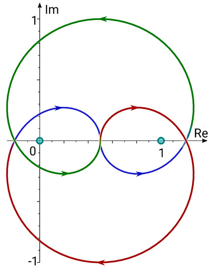Figure 1. The integration curve for the Jacobi weight when $\alpha ,\beta \in \mathbb{C}\backslash \mathbb{Z}$. The colors correspond to continuous branches of $z^{\alpha }$ and ${(1-z)}^{\beta }$: the principal branches are in blue, blue changes to green as ${(1-z)}^{\beta }$ passes to another branch, and green changes to red as $z^{\alpha }$ passes to another branch. Note that $z^{\alpha }{(1-z)}^{\beta }$ is continuous on the whole curve.

(b’)

The Bessel weight $z^{\alpha }{e}^{1/z}$, when $\sigma \left(z\right)=z^2$ has a double zero, so $\tau \left(z\right)=(2+\alpha )z-1$. The curve $\Gamma$ here is the cardioid $\Gamma ={\Gamma }^B=\left\{{(e^{it}-1)}^2:t\in (0,2\pi )\right\}$. For $\alpha \in \mathbb{Z}$, one can also take ${\Gamma }^B$ to be the unit circle ${\Gamma }^B=\{z:|z|=1\}$.

(c’)

The Laguerre weight $z^{\alpha }{e}^{-z}$, when $\sigma \left(z\right)=z$, so $\tau \left(z\right)=-z+\alpha +1$. Here we take $\Gamma ={\Gamma }_{\alpha }^L$ to be either the positive semi-axis, or a parabola encircling it:

$$\Gamma =\left\{\begin{array}{cc}(0,+\infty ),\hfill & \mathrm{if}\Re \alpha >-1;\hfill \\ \left\{-{(e^{-it}-1)}^{-2}:t\in (0,2\pi )\right\},\hfill & \mathrm{if}\alpha \in \mathbb{C}\backslash {\mathbb{Z}}_{⩾0}.\hfill \end{array}\right.$$

(d’)

The Hermite weight $e^{-z^2}$, when $\sigma \left(z\right)\equiv 1$, and hence $\tau \left(z\right)=-2z$. Here we put $\Gamma ={\Gamma }^H=(-\infty ,+\infty )$.

Proposition 1. 

The weight w is quasi-definite on the curve Γ defined above in the following cases:

• If and only if $\alpha ,\beta ,\alpha +\beta +1\in \mathbb{C}\backslash {\mathbb{Z}}_{<0}$ in the case (a’);
• If and only if $\alpha +1\in \mathbb{C}\backslash {\mathbb{Z}}_{<0}$ in the case (b’);
• If and only if $\alpha \in \mathbb{C}\backslash {\mathbb{Z}}_{<0}$ in the case (c’);
• In the case (d’).

Remark 1. 

In all cases (a’)–(d’), the corresponding orthogonal polynomial $P_n\left(z\right)$ may be found via Rodrigues’s formula:

$$P_n\left(z\right)=\frac{\mathrm{const}}{w\left(z\right)}·\frac{d^n}{d{z}^n}\left({\sigma }^n\left(z\right)w\left(z\right)\right).$$

(7)

Here the index $n\in {\mathbb{Z}}_{⩾0}$ is the scalar.

Proposition 1 mostly contains known results: for instance, [24] (Theorem 3.2) derives the quasi-definiteness in the Jacobi case $\left(a^{\prime }\right)$ from the uniqueness of the solution of the corresponding matrix Riemann–Hilbert problem. Our Proposition 1 is a particular case of the more general result stated in the next section devoted to multiple orthogonality.

2.1.2. Multiple Continuous Weights

In the general case $r⩾1$, possible weights solving the Pearson’s equation in (5) clearly coincide with those listed above in $\left(a^{\prime }\right)$–$\left(d^{\prime }\right)$. Moreover, since all weights $w_1,\dots ,w_r$ share the same polynomial $\sigma$, only combinations of same-type weights are possible. Nevertheless, the contours may (and in some situations must) be different. The details will be clear below.

It is shown in [17] that, for some of the combinations of weights, Rodrigues’s operators (appearing on the right-hand side of (7)) commute, and hence their compositions yield Rodrigues’s formulae, producing the corresponding multiple orthogonal polynomials. The authors of [17] identified combinations (up to a linear transform of the variable and normalization) with commuting Rodrigues’s operators. For $j=1,\dots ,r$, we have the following:

(a)

The system of weights $w_j\left(z\right)=z^{{\alpha }_j}{(1-z)}^{\beta }$ on curves ${\Gamma }_j={\Gamma }_{{\alpha }_j,\beta }^J$ defines the Jacobi-Piñeiro polynomials;

(b)

The system of weights $w_j\left(z\right)=z^{{\alpha }_j}{e}^{1/z}$ on curves ${\Gamma }_j={\Gamma }^B$ defines the multiple Bessel polynomials;

(c)

The system of weights $w_j\left(z\right)=z^{{\alpha }_j}{e}^{-z}$ on curves ${\Gamma }_j={\Gamma }_{{\alpha }_j}^L$ defines the multiple Laguerre I polynomials;

(d)

The system of weights $w_j\left(z\right)=e^{-z^2-{\gamma }_{j}z}$ on curves ${\Gamma }_j={\Gamma }^H$ defines the multiple Hermite polynomials;

(e)

The system of weights $w_j\left(z\right)=z^{\beta }{e}^{-{\gamma }_{j}z}$, ${\gamma }_j\ne 0$, on curves ${\Gamma }_j={\gamma }_j^{-1}·{\Gamma }_{\beta }^L$ defines the multiple Laguerre II polynomials.

Theorem 1. 

Let a system of weights $w_1,\dots ,w_r$ on curves ${\Gamma }_1,\dots ,{\Gamma }_r$ be as one of those defined in (a)–(e). This system is perfect if and only if the following hold:

• ${\alpha }_k-{\alpha }_j\in \mathbb{C}\backslash \mathbb{Z}$ and ${\alpha }_k,\beta ,{\alpha }_k+\beta +1\in \mathbb{C}\backslash {\mathbb{Z}}_{<0}$ in the case (a);
• ${\alpha }_k-{\alpha }_j\in \mathbb{C}\backslash \mathbb{Z}$ and ${\alpha }_k+1\in \mathbb{C}\backslash {\mathbb{Z}}_{<0}$ in the case (b);
• ${\alpha }_k-{\alpha }_j\in \mathbb{C}\backslash \mathbb{Z}$ and ${\alpha }_k\in \mathbb{C}\backslash {\mathbb{Z}}_{<0}$ in the case (c);
• ${\gamma }_k\ne {\gamma }_j$ and ${\gamma }_k\in \mathbb{C}$ in the case (d);
• $\beta \in \mathbb{C}\backslash {\mathbb{Z}}_{<0}$ and ${\gamma }_k\ne {\gamma }_j$, ${\gamma }_k\in \mathbb{C}\backslash \left\{0\right\}$ in the case (e)

for all $k,j=1,\dots ,r$ with $k\ne j$.

Remark 2. 

It is known [17], and we show it in Section 4 that orthogonal polynomials for the systems of weights listed in (a)–(e) may be found through Rodrigues’s formula

$$P_{\mathit{n}}\left(z\right)=\left\{\begin{array}{cc}{\displaystyle \frac{\mathrm{const}}{w_1\left(z\right)}\left(\prod _{j=1}^{r-1}\frac{d^{n_j}}{d{z}^{n_j}}{z}^{{\alpha }_j+n_j-{\alpha }_{j+1}}\right)\frac{d^{n_r}}{d{z}^{n_r}}{\left(\frac{\sigma \left(z\right)}{z}\right)}^{\left|\mathit{n}\right|}{z}^{n_r}{w}_r\left(z\right)}\hfill & \mathit{for}\mathit{\left(}a\mathit{\right)}\mathit{–}\mathit{\left(}\mathit{c}\mathit{\right)}\mathit{;}\hfill \\ {\displaystyle \frac{\mathrm{const}}{w_1\left(z\right)}\left(\prod _{j=1}^{r-1}\frac{d^{n_j}}{d{z}^{n_j}}{e}^{({\gamma }_{j+1}-{\gamma }_j)z}\right)\frac{d^{n_r}}{d{z}^{n_r}}{\sigma }^{\left|\mathit{n}\right|}\left(z\right)w_r\left(z\right)}\hfill & \mathit{for}\mathit{\left(}\mathit{d}\mathit{\right)}\mathit{–}\mathit{\left(}\mathit{e}\mathit{\right)}\mathit{,}\hfill \end{array}\right.$$

(8)

where the factors in the products are differential operators.

The Jacobi–Piñeiro case was considered in [28], where the perfectness was deduced from an explicit formula for the determinant $D_{\mathit{n}}$ defined in (13) below.

2.2. Weights Satisfying Difference Pearson’s Equation

Under $\Delta$ and ∇, we understand the forward and backward finite differences, respectively:

$$\Delta f\left(z\right)=f(z+1)-f\left(z\right),\nabla f\left(z\right)=f\left(z\right)-f(z-1).$$

Consider r meromorphic in $\mathbb{C}$ functions $w_1,\dots ,w_r$ satisfying difference Pearson’s equation

$$\Delta \left(\sigma \left(z\right)w_j\left(z\right)\right)={\tau }_j\left(z\right)w_j\left(z\right)$$

(9)

where $\sigma$ and ${\tau }_j$ are polynomials such that $deg\sigma ⩽2$ and $deg{\tau }_j⩽1$, $j=1,\dots ,r$. Let us note that the solutions of (9) are defined up to a multiplier, which can be an arbitrary meromorphic function with period 1.

We will consider two kinds of functionals. The first kind is defined by a complex measure with discrete support:

$$l_j\left(Q\right):=\sum _{x=0}^{N}Q\left(x\right)w_j\left(x\right)=\int Q\left(z\right)d{\mu }_j\left(z\right),{\mu }_j\left(z\right):=\sum _{x=0}^N{w}_j\left(x\right)\delta (z-x),$$

where $\delta$ is the Dirac delta function, and $N\in {\mathbb{Z}}_{>0}\cup \{\infty \}$. The second kind of functionals is

$$l_j\left(Q\right):={\int }_{L_j}Q\left(z\right){\tilde{w}}_j\left(z\right)dz,$$

where ${\tilde{w}}_j$ stands for some other solution of (9), i.e., $\Delta \frac{w_j}{{\tilde{w}}_j}\equiv 0$, and $L_j$ is a smooth curve in $\mathbb{C}$ encircling the support of discrete measure ${\mu }_j$ so that either it is closed, or both its ends are at infinity. The current section is devoted to multiple orthogonal polynomials with respect to the above functionals.

2.2.1. One Weight

It is well known (see Table 2) that there are four types of nontrivial weights satisfying the difference Pearson’s Equation (4). There are four families of classical discrete orthogonal polynomials, namely the Charlier, Meixner, Krawtchouk and Hahn polynomials. For standard parameters, the Charlier and Meixner weights are supported on an infinite set ${\mathbb{Z}}_{+}$, while the Krawtchouk and Hahn polynomials are supported on the finite set $\{0,1,\dots ,N\}$ of integers. These four families can be characterized by a difference version of Rodrigues’s formula.

Table 2. Weights for classical orthogonal polynomials of discrete variable.

	Hahn	Krawtchouk	Meixner	Charlier
$w\left(x\right)$	${\displaystyle \frac{{(\alpha +1)}_x{(\beta +1)}_{N-x}}{\Gamma (x+1)\Gamma (N-x+1)}}$	$\frac{{\displaystyle b^x\phantom{|}}}{\phantom{|}\Gamma (x+1)\Gamma (N-x+1)}$	${\displaystyle \frac{b^x\Gamma (x+\alpha )}{\Gamma (x+1)}}$	${\displaystyle \frac{b^x}{\Gamma (x+1)}}$
$\sigma \left(x\right)$	$x(N-x+\beta +1)$	x	x	x
$\tau \left(x\right)+\sigma \left(x\right)$	$(x+\alpha +1)(N-x)$	$b(x+\alpha )$	$b(N-x)$	b
Standard parameters	$\alpha ,\beta >-1$, $N\in {\mathbb{Z}}_{>0}$	$b>0$, $N\in {\mathbb{Z}}_{>0}$	$\alpha >0,0<b<1$	$b>0$

Let us list these weights and integration contours for all (including nonstandard) parameters. We use the notation

$${\left(a\right)}_x=\Gamma (a+x)/\Gamma \left(a\right)$$

for the Pochhammer symbol; for $x\in {\mathbb{Z}}_{>0}$, it reduces to ${\left(a\right)}_x=a·(a+1)\cdots (a+x-1)$.

(i’)

The Hahn weight is

$$w\left(z\right)=\frac{{(\alpha +1)}_z{(\beta +1)}_{N-z}}{\Gamma (z+1)\Gamma (N-z+1)}$$

and $\mu$ is defined and supported on $\{0,\dots ,N\}$ if $N\in Z_{>0}$. Furthermore,

$$\tilde{w}\left(z\right):=\Gamma (z+\alpha +1)\Gamma (z-N)\Gamma (-z)\Gamma (N-z+\beta +1).$$

Under the conditions

$$\alpha +1,\beta +1,(\alpha +\beta +N+2),-N\in \mathbb{C}\backslash {\mathbb{Z}}_{⩽0},$$

(10)

we consider the curve $L=L_{\alpha ,\beta ,N}^H$ ending at $\pm i\infty$ and separating $\{-\alpha -1,-\alpha -2,\dots \}\cup \{N,N-1,\dots \}$ from $\{\beta +N+1,\beta +N+2,\dots \}\cup \{0,1,\dots \}$.

If any of the parameters violates (10), then without loss of generality, it is enough only to consider the case $N\in {\mathbb{Z}}_{⩾0}$. Indeed, the continuous weight $\tilde{w}\left(z\right)$ still corresponds to the discrete weight $w\left(z\right)$ or $w(N-z)$ after relabeling its parameters. For instance, it corresponds to $w\left(z\right)$ on exchanging $\alpha +1\leftrightarrow -N$ and $\beta \leftrightarrow \beta +N-\alpha -1$ in the case $\alpha +1\in {\mathbb{Z}}_{⩽0}$.

(ii’)

The Krawtchouk weight is

$$w\left(z\right)=\frac{{\displaystyle b^z\phantom{|}}}{\phantom{|}\Gamma (z+1)\Gamma (N-z+1)}$$

and $\mu$ is defined and supported on $\{0,\dots ,N\}$ if $N\in Z_{⩾0}$. Let us note that the Krawtchouk weight transforms into the Meixner weight after $(b,N)\to (-b,-\alpha )$. So the nonstandard parameters can be found in the next entry (iii’).

(iii’)

The Meixner weight is

$$w\left(z\right)=\frac{b^z\Gamma (z+\alpha )}{\Gamma (z+1)}.$$

For $0<\left|b\right|<1$ the measure $\mu$ is suppoted on ${\mathbb{Z}}_{⩾0}$. Let $\alpha \notin {\mathbb{Z}}_{⩽0}$ and $b\notin \{0,1\}$. Put

$$\tilde{w}\left(z\right)=\frac{\pi e^{i\pi z}}{sin\left(\pi z\right)}w\left(z\right)={(-b)}^z\Gamma (z+\alpha )\Gamma (-z).$$

Unless $b>0$, the curve $L=L_{b,\alpha }^M$ is defined analogously to the Hahn case, namely it separates $\{-\alpha ,-\alpha -1,\dots \}$ from $\{0,1,\dots \}$ and ends at $\pm i\infty$. For $\left|b\right|\ne 1$, we can take the curve $L=L_{b,\alpha }^M$ with the ends at infinity in the closed halfplane where ${(-b)}^z$ is bounded and still separating $\{-\alpha ,-\alpha -1,\dots \}$ from $\{0,1,\dots \}$.

(iv’)

The Charlier weight is

$${\displaystyle w\left(z\right)=\phantom{\frac{\left|}{\right|}}\frac{b^z}{\Gamma (z+1)},}$$

with the only condition $b\ne 0$. The discrete measure of orthogonality $\mu$ is supported on ${\mathbb{Z}}_{⩾0}$.

Proposition 2. 

The functional l corresponding to one of the weights described above in (i’)–(iv’) is quasi-definite if and only if

(i’)

$\alpha +1,\beta +1,\alpha +\beta +N+2,-N\in \mathbb{C}\backslash {\mathbb{Z}}_{⩽0}$ for the Hahn weight;

(ii’)

$b\in \mathbb{C}\backslash \{0,-1\}$ and $N\in \mathbb{C}\backslash {\mathbb{Z}}_{⩾0}$ for the Krawtchouk weights;

(iii’)

$\alpha \in \mathbb{C}\backslash {\mathbb{Z}}_{⩽0}$ and $b\in \mathbb{C}\backslash \{0,1\}$ for the Meixner weight;

(iv’)

$b\in \mathbb{C}\backslash \left\{0\right\}$ for the Charlier weight.

Given that $N\in {\mathbb{Z}}_{>0}$ in the cases (i’) and (ii’), all indices $n⩽N$ for the corresponding system of orthogonal polynomials are normal if and only if

• $\alpha ,\beta \in \mathbb{C}\backslash \{-1,-2,\dots ,1-N\}$, $\alpha +\beta \in \mathbb{C}\backslash \{-2,-3,\dots ,-2N\}$ in (i’), and
• $b\in \mathbb{C}\backslash \{0,-1\}$ in (ii’).

This proposition is a particular case of Theorem 2 from the next section.

2.2.2. Multiple Weights

Analogously to Section 2.1.2, the general case $r⩾1$ only allows certain combinations of same-type weights solving the difference Pearson’s equation (9), because all weights $w_1,\dots ,w_r$ are supposed to share the same polynomial $\sigma$. Just like in the continuous case, we consider the orthogonality with respect to several functionals $l_j$, where each $l_j$ is already defined in the previous paragraph. There are several families of multiple orthogonal polynomials corresponding to the system $l_j$ and retaining Rodrigues’s formula: the multiple Charlier, multiple Meixner I and II, multiple Krawtchouk and multiple Hahn polynomials (see [33]).

The multiple Charlier polynomials correspond to $N=\infty$ and $w_j\left(x\right)=\frac{b_j^x}{\Gamma (x+1)}$. The multiple Hahn polynomials correspond to $w_{N,j}^{(\mathbf{\alpha },\beta )}\left(x\right)=\frac{{({\alpha }_j+1)}_x\Gamma {(\beta +1)}_{N-x}}{\Gamma (x+1)\Gamma (N-x+1)}$; for non-integer values of N we arrive at the multiple continuous Hahn polynomials. The multiple Krawtchouk polynomials correspond to $w_{N,j}^{\left(\mathit{b}\right)}\left(x\right)=\frac{b_j^x}{\Gamma (x+1)\Gamma (N-x+1)}$. In fact, for non-integer values of N, they can be reduced to the multiple Meixner polynomials.

The most involved cases are the multiple Meixner polynomials. Indeed, the weights $w_j^{(\alpha ,\mathit{b})}\left(x\right)=\frac{b_j^x\Gamma (x+\alpha )}{\Gamma (x+1)}$ for the Meixner I polynomials for $\alpha \in {\mathbb{Z}}_{⩽0}$ transform to the Krawtchouk weights for $N=-\alpha$. If $|b_j|<1$, then we have discrete orthogonality on ${\mathbb{Z}}_{⩾0}$. If $|b_j|>1$, then we introduce a change of variable $b_j\to 1/b_j,x\to -x-\alpha$, cf. ([10], p. 177, Equation (3.6)). If $|b_j|=1$ and $b_j\ne 1$, then we need to consider the Meixner–Pollaczek polynomials, cf. ([10], p. 180, Equations (3.17), (3.21), and (3.22)). Similarly, one or several weights $w_j^{(\mathbf{\alpha },b)}\left(x\right)=\frac{b^x\Gamma (x+{\alpha }_j)}{\Gamma (x+1)}$ for the multiple Meixner II polynomials with ${\alpha }_j\in {\mathbb{Z}}_{⩽0}$ transform to the Krawtchouk weights. Furthermore, depending on $\left|b\right|$, one can consider discrete or continuous orthogonality. We treat the Meixner weights in more detail in Section 5.1.

Theorem 2. 

The systems of functionals $l_1,\dots ,l_r$ generating multiple orthogonal polynomials are perfect if and only if

(i)

${\alpha }_k+1,\beta +1,{\alpha }_k+\beta +N+2,-N\in \mathbb{C}\backslash {\mathbb{Z}}_{⩽0}$, as well as ${\alpha }_j-{\alpha }_k\notin \mathbb{Z}$ as $j\ne k$ for the multiple Hahn weights;

(ii)

$b_j\in \mathbb{C}\backslash \{0,-1\}$, $N\in \mathbb{C}\backslash {\mathbb{Z}}_{⩾0}$ and $b_j\ne b_k$ as $j\ne k$ for the multiple Krawtchouk weights;

(iii)

$b_j\in \mathbb{C}\backslash \{0,1\}$ and $\alpha \in \mathbb{C}\backslash {\mathbb{Z}}_{⩽0}$, as well as $b_j\ne b_k$ as $j\ne k$ for the multiple Meixner I weights;

(iv)

$b_j\in \mathbb{C}\backslash \left\{0\right\}$ and $b_j\ne b_k$ as $j\ne k$ for the multiple Charlier weights;

(v)

$b\in \mathbb{C}\backslash \{0,1\}$ and ${\alpha }_k\in \mathbb{C}\backslash {\mathbb{Z}}_{⩽0}$, in addition to ${\alpha }_j-{\alpha }_k\notin \mathbb{Z}$ as $j\ne k$ for the multiple Meixner II weights.

Given that $N\in {\mathbb{Z}}_{>0}$ in the cases (i) and (ii), all indices $\left|\mathit{n}\right|⩽N$ for the corresponding system of orthogonal polynomials are normal if and only if

• ${\alpha }_k,\beta \in \mathbb{C}\backslash \{-1,-2,\dots ,1-N\}$, ${\alpha }_k+\beta \in \mathbb{C}\backslash \{-2,-3,\dots ,-2N\}$ simultaneously with ${\alpha }_j-{\alpha }_k\notin \{-N+1,-N+2,\dots ,N-1\}$ as $j\ne k$ in (i), and
• $b_k\in \mathbb{C}\backslash \{0,-1\}$ together with $b_j\ne b_k$ as $j\ne k$ in (ii).

Remark 3. 

In the last theorem, in the cases (i) and (ii) with $N\in {\mathbb{Z}}_{⩾0}$, only the indices satisfying $\left|\mathit{n}\right|⩽N+1$ may be normal: indeed, the polynomial ${(x-N)}_{N+1}$ of degree $N+1$ is orthogonal to monomials of all non-negative integer degrees. An analogous remark may be applied to the case (iii) when $\alpha \in {\mathbb{Z}}_{⩽0}$ and to the case (v) when ${\alpha }_j\in {\mathbb{Z}}_{⩽0}$ and $n_j⩽-{\alpha }_j$.

Analogously to the continuous case, we show that the difference Rodrigues’s formula (25) given below produces the orthogonal polynomials under the conditions of Theorem 2. Up to normalization, this formula coincides with Rodrigues’s formula obtained in [33] for standard values of the parameters.

2.3. Nearest-Neighbor Recurrence and Perfectness

It is known that, if $\mathit{n}$ and $\mathit{n}+{\mathit{e}}_k$ are normal indices, then the monic multiple orthogonal polynomials satisfy the so-called nearest neighbor recurrence relations:

$$x{P}_{\mathit{n}}\left(x\right)=P_{\mathit{n}+{\mathit{e}}_k}\left(x\right)+b_{\mathit{n},k}{P}_{\mathit{n}}\left(x\right)+\sum _{j=1}^r{a}_{\mathit{n},j}{P}_{\mathit{n}-{\mathit{e}}_j}\left(x\right),$$

(11)

where $P_{\mathit{n}-{\mathit{e}}_j}=0$ when $n_j=0$, and

$$a_{\mathit{n},j}=\left\{\begin{array}{cc}{l}_j\left(x^{n_j}{P}_{\mathit{n}}\right)/l_j\left(x^{n_j-1}{P}_{\mathit{n}-{\mathit{e}}_j}\right),\hfill & \mathrm{if}{n}_j\ne 0,\hfill \\ 0,\hfill & \mathrm{if}{n}_j=0\hfill \end{array}\right.$$

and a similar representation for $b_{\mathit{n},k}$ uses type-I multiple polynomials; see ([39], Theorem 23.1.11) and [40] for the details. The converse (in a sense) to this assertion is presented by the following fact, whose proof given below uses methods similar to those of Theorem 1.

Proposition 3. 

For every $\mathit{n}\in {\mathbb{Z}}_{+}^r$, let there be some polynomial $P_{\mathit{n}}$ of degree $\left|\mathit{n}\right|$ satisfying the orthogonality conditions (1), such that

$$x{P}_{\mathit{n}}\left(x\right)=P_{\mathit{n}+{\mathit{e}}_{k\left(\mathit{n}\right)}}\left(x\right)+b_{\mathit{n}}{P}_{\mathit{n}}\left(x\right)+\sum _{j=1}^r{a}_{\mathit{n},j}{P}_{\mathit{n}-{\mathit{e}}_j}\left(x\right)$$

(12)

holds for some $k\left(\mathit{n}\right)\in \{1,\dots ,r\}$ and some complex numbers $b_{\mathit{n}}$ and $a_{\mathit{n},j}$, where we put $a_{\mathit{n},j}{P}_{\mathit{n}-{\mathit{e}}_j}\left(x\right)$$\equiv 0$ as $n_j=0$. Then this system of functionals $l_1,\dots ,l_r$ is perfect if and only if for $j=1,\dots ,r$ the values of $a_{\mathit{n},j}$ are nonzero whenever $n_j\ne 0$, as well as $l_j\left(P_{\mathbf{\nu }}\right)\ne 0$ for $\mathbf{\nu }=({\nu }_1,\dots {\nu }_r)\in {\{0,1\}}^r$ with ${\nu }_j=0$.

Note that, if for every $\mathit{n}\in {\mathbb{Z}}_{⩾0}^r$ the relation (12) holds not only for some $k\left(\mathit{n}\right)$, but for all $k=1,\dots ,r$ as in (11), then each $P_{\mathit{n}}$ is automatically a monic polynomial of degree $\left|\mathit{n}\right|$ provided that $P_{(0,\dots ,0)}\left(x\right)\equiv 1$.

3. Basic Theory

We introduce a notation ${\mathcal{O}}_{\mathit{n}}$ for all nontrivial polynomials of $\mathrm{deg}{P}_{\mathit{n}}⩽\left|\mathit{n}\right|,$ satisfying (1). Clearly, ${\mathcal{O}}_{\mathit{n}}\cup \left\{0\right\}$ is a linear space of positive dimension. Let us now review some basic facts related to normality and perfectness.

We say that a $k_1\times k_2$ matrix A is a Hankel matrix if its entries on each antidiagonal are equal, that is, if it can be written as $A={\left(a_{i+j}\right)}_{i,j=1}^{k_1,k_2}$. Given an index $\mathit{n}\in {\mathbb{Z}}_{⩾0}^r$ and $s_{j,k}=l_j\left(z^{k-1}\right)$—the moments of functionals $l_j$, put

$$H_{\mathit{n}}:=\left[\begin{array}{cccc}{s}_{1,1}& s_{1,2}& \dots & s_{1,\left|\mathit{n}\right|}\\ s_{1,2}& s_{1,3}& \dots & s_{1,\left|\mathit{n}\right|+1}\\ ⋮& ⋮& \ddots & ⋮\\ s_{1,n_1}& s_{1,n_1+1}& \dots & s_{1,\left|\mathit{n}\right|+n_1-1}\\ s_{2,1}& s_{2,2}& \dots & s_{2,\left|\mathit{n}\right|}\\ ⋮& ⋮& \ddots & ⋮\\ s_{r,n_r}& s_{r,n_r+1}& \dots & s_{r,\left|\mathit{n}\right|+n_r-1}\end{array}\right]\mathrm{and}{D}_{\mathit{n}}:=det{H}_{\mathit{n}}(D_{(0,\dots ,0)}=1),$$

(13)

so that $D_{\mathit{n}}$ is a determinant of order $\left|\mathit{n}\right|$ containing r rectangular Hankel blocks of sizes $n_1\times \left|\mathit{n}\right|,n_2\times \left|\mathit{n}\right|,\dots ,n_r\times \left|\mathit{n}\right|$. It turns out that the condition $D_{\mathit{n}}\ne 0$ is necessary and sufficient for the normality of $\mathit{n}$; see Lemma 1 below.

Lemma 1 

(see, for example, ([39], §23.1) or [11]). Let $l_1,\dots ,l_r$ be linear functionals $\mathbb{C}\left[z\right]\to \mathbb{C}$. Then the normality of an index $\mathit{n}$ is equivalent to $D_{\mathit{n}}\ne 0$, where $D_{\mathit{n}}$ is the determinant defined in (13).

Proof. 

Observe that for a polynomial $P_{\mathit{n}}\left(x\right)={\sum }_{k=0}^{\left|\mathit{n}\right|}{c}_k{z}^k$, the orthogonality conditions (1) may be written as

$$H_{\mathit{n}}·{\left[c_0,c_1,\dots ,c_{\left|\mathit{n}\right|-1}\right]}^T=-c_{\left|\mathit{n}\right|}·{\left[s_{1,\left|\mathit{n}\right|+1},\dots ,s_{1,\left|\mathit{n}\right|+n_1},s_{2,\left|\mathit{n}\right|+1},\dots ,s_{r,\left|\mathit{n}\right|+n_r}\right]}^T,$$

and for $D_{\mathit{n}}\ne 0$, this linear system has a unique solution. So, the orthogonal polynomial $P_{\mathit{n}}\left(x\right)={\sum }_{k=0}^{\left|\mathit{n}\right|}{c}_k{z}^k$ in this case is defined uniquely up to multiplication by a nonzero constant, and hence $\mathit{n}$ is normal. On fixing $c_{\left|\mathit{n}\right|}=D_{\mathit{n}}$, Cramer’s rule yields

$$P_{\mathit{n}}\left(x\right):=\left|\begin{array}{cccc}{s}_{1,1}& s_{1,2}& \dots & s_{1,\left|\mathit{n}\right|+1}\\ s_{1,2}& s_{1,3}& \dots & s_{1,\left|\mathit{n}\right|+2}\\ ⋮& ⋮& \ddots & ⋮\\ s_{1,n_1}& s_{1,n_1+1}& \dots & s_{1,\left|\mathit{n}\right|+n_1}\\ s_{2,1}& s_{2,2}& \dots & s_{2,\left|\mathit{n}\right|+1}\\ ⋮& ⋮& \ddots & ⋮\\ s_{r,n_r}& s_{r,n_r+1}& \dots & s_{r,\left|\mathit{n}\right|+n_r}\\ 1& x& \dots & x^{\left|\mathit{n}\right|}\end{array}\right|=\left|\begin{array}{cccc}& & & s_{1,\left|\mathit{n}\right|+1}\\ & & & s_{1,\left|\mathit{n}\right|+2}\\ & H_{\mathit{n}}& & ⋮\\ & & & s_{r,\left|\mathit{n}\right|+n_r}\\ 1& x& \dots & x^{\left|\mathit{n}\right|}\end{array}\right|.$$

(14)

At the same time, for $D_{\mathit{n}}=0$, the orthogonality conditions (1) can be satisfied by a polynomial of degree strictly less than $\left|\mathit{n}\right|$, namely, by $P_{\mathit{n}}\left(x\right)={\sum }_{k=0}^{\left|\mathit{n}\right|-1}{c}_k{z}^k$ for any nontrivial solution $c_0,\dots ,c_{\left|\mathit{n}\right|-1}$ of the homogeneous system

$$H_{\mathit{n}}·{\left[c_0,c_1,\dots ,c_{\left|\mathit{n}\right|-1}\right]}^T={\left[0,0,\dots ,0\right]}^T.$$

Therefore, the index $\mathit{n}$ in this case is not normal. □

Remark 4. 

Let us point out that the right-hand side of (14) satisfies the orthogonality conditions (1) regardless of whether $D_{\mathit{n}}$ vanishes or not. So, for $D_{\mathit{n}}=0$ and $P_{\mathit{n}}\left(x\right)$ defined from (14), the condition $P_{\mathit{n}}\left(x\right)\not\equiv 0$ is equivalent to that $P_{\mathit{n}}\left(x\right)$ is the only solution of (1) up to multiplication by a nonzero constant. For instance, if $r=1$ and $l\left(Q\right)=Q\left(0\right)+Q^{\prime }\left(0\right)+Q^{″}\left(0\right)/2$, then for $n=2$ every polynomial of degree $⩽2$ satisfying (1) is equal to $x-1$ times some constant.

The next fact on perfectness is a variant of ([28], Lemma 3.4).

Lemma 2. 

Let $N\in {\mathbb{Z}}_{⩾0}\cup \{\infty \}$. For the linear functionals $l_1,\dots ,l_r$ to have all indices $\mathit{n}$, $\left|\mathit{n}\right|⩽N$, normal (and to form a perfect system when $N=\infty$), it is necessary and sufficient that for each index $\mathit{n}\in {\mathbb{Z}}_{⩾0}^r$ with $\left|\mathit{n}\right|⩽N$, there exists a polynomial $P_{\mathit{n}}\in {\mathcal{O}}_{\mathit{n}}$ of degree $\left|\mathit{n}\right|$ such that for $\left|\mathit{n}\right|<N$ it satisfies $P_{\mathit{n}}\notin {\bigcup }_{k=1}^r{\mathcal{O}}_{\mathit{n}+{\mathit{e}}_k}$.

Proof. 

The “only if” part follows directly from the definition of normality. The “if” part follows by induction in $\left|\mathit{n}\right|$. For the base of the induction, observe that the index $(0,\dots ,0)$ is always normal, as the corresponding orthogonal polynomial is not supposed to obey any orthogonality conditions.

Now, suppose that the index $\mathit{n}$ with $0<\left|\mathit{n}\right|⩽N$ is not normal, while all indices $\mathbf{\nu }$ satisfying $\left|\mathbf{\nu }\right|<\left|\mathit{n}\right|$ are normal. Then there is a polynomial $Q\in {\mathcal{O}}_{\mathit{n}}$ of degree $m<\left|\mathit{n}\right|$. Moreover, there is also some $k\in \{1,\dots ,r\}$ and index $\mathbf{\nu }=({\nu }_1,\dots ,{\nu }_r)$ satisfying $\left|\mathbf{\nu }\right|=m$, as well as ${\nu }_j+{\delta }_{j,k}⩽n_j$ for $j=1,\dots ,r$ with ${\delta }_{j,k}$ denoting the Kronecker delta such that $Q\in {\mathcal{O}}_{\mathbf{\nu }}$. Consequently, the normality of $\mathbf{\nu }$ implies that $P_{\mathbf{\nu }}$ must coincide with Q up to multiplication by a constant. The equality $Q=\mathrm{const}·P_{\mathbf{\nu }}$ is, however, impossible because $Q\in {\mathcal{O}}_{\mathit{n}}$ and $P_{\mathbf{\nu }}\notin {\mathcal{O}}_{\mathbf{\nu }+{\mathit{e}}_k}$. So, the index $\mathit{n}$ can only be normal. By induction, we prove the normality of all the indices $\mathit{n}$ with $\left|\mathit{n}\right|⩽N$. □

Another proof of Lemma 2. 

The “only if” part follows directly from the definition of normality. The “if” part follows by induction in $\left|\mathit{n}\right|$. For the base of the induction, observe that the index $(0,\dots ,0)$ is always normal, as the corresponding orthogonal polynomial is not supposed to obey any orthogonality conditions.

Now, suppose that the index $\mathit{n}+{\mathit{e}}_k$ with $\left|\mathit{n}\right|<N$ for some $k\in \{1,\dots ,r\}$ is not normal, while the index $\mathit{n}$ is normal. Then $D_{\mathit{n}}\ne 0$ and $D_{\mathit{n}+{\mathit{e}}_k}=0$. Write the orthogonal polynomial $P_{\mathit{n}}$ via the determinant formula (14), then $l_k\left(P_{\mathit{n}}{x}^{n_k}\right)=D_{\mathit{n}+{\mathit{e}}_k}=0$, which contradicts to $P_{\mathit{n}}\notin {\mathcal{O}}_{\mathit{n}+{\mathit{e}}_k}$. □

Proof of Proposition 3

Observe that if for a polynomial Q the conditions $Q\in {\mathcal{O}}_{\mathit{n}}$ and $l_j\left(x^{n_j}Q\right)=0$ are simultaneously satisfied, then $Q\in {\mathcal{O}}_{\mathit{n}+{\mathit{e}}_j}$. Therefore, by Lemma 2 the perfectness is equivalent to that $l_j\left(x^{n_j}{P}_{\mathit{n}}\right)\ne 0$ for all $j=1,\dots ,r$ and $\mathit{n}\in {\mathbb{Z}}_{+}^r$.

On multiplying (12) for $n_j>0$ by $x^{n_j-1}$ and then acting by $l_j$, we arrive at

$$l_j\left(x^{n_j}{P}_{\mathit{n}}\right)=a_{\mathit{n},j}{l}_j\left(x^{n_j-1}{P}_{\mathit{n}-{\mathit{e}}_j}\right).$$

(15)

In particular, the “only if” assertion of the proposition immediately follows from this identity: $a_{\mathit{n},j}=0$ for some $\mathit{n}$ and j implies absence of the perfectness by Lemma 2, while the conditions $l_j\left(P_{\mathbf{\nu }}\right)\ne 0$ for $\mathbf{\nu }=({\nu }_1,\dots {\nu }_r)\in {\{0,1\}}^r$ with ${\nu }_j=0$ are clearly necessary for perfectness.

For the “if” assertion, observe that all indices satisfying $\left|\mathit{n}\right|⩽1$ are normal: trivially when $\left|\mathit{n}\right|=0$, and by the proposition’s assumption $l_j\left(1\right)\ne 0$ when $\left|\mathit{n}\right|=1$. By induction in $N\in {\mathbb{Z}}_{>0}$, let us show that each index $\mathit{n}$ with $\left|\mathit{n}\right|=N+1$ is normal provided that all indices satisfying $\left|\mathit{n}\right|⩽N$ are normal. According to Lemma 2, it is enough to prove that $l_j\left(x^{n_j}{P}_{\mathit{n}}\right)\ne 0$ for all j and $\mathit{n}$ with $\left|\mathit{n}\right|=N$. For each j such that $n_j>0$, we immediately have $l_j\left(x^{n_j}{P}_{\mathit{n}}\right)\ne 0$ due to (15). The case $n_j=0$ and $n_k⩽1$ for all k follows from the proposition’s conditions.

Now, let $n_j=0$ and $n_k⩾2$ for some k. Then $l_j(x^{n_j}·P_{\mathit{n}})=0$ would mean that $P_{\mathit{n}}\in {\mathcal{O}}_{\mathit{n}+{\mathit{e}}_j}$, and hence $P_{\mathit{n}}\in {\mathcal{O}}_{\mathit{n}+{\mathit{e}}_j-{\mathit{e}}_k}$. Due to the normality of the index $\mathit{n}+{\mathit{e}}_j-{\mathit{e}}_k$, the polynomial $P_{\mathit{n}}$ then would be identically equal to $P_{\mathit{n}+{\mathit{e}}_j-{\mathit{e}}_k}$ up to normalization. That would mean that $P_{\mathit{n}+{\mathit{e}}_j-{\mathit{e}}_k}\in {\mathcal{O}}_{\mathit{n}+{\mathit{e}}_j}$ and

$$0=l_k\left(x^{n_k-1}{P}_{\mathit{n}+{\mathit{e}}_j-{\mathit{e}}_k}\right)=a_{\mathit{n}+{\mathit{e}}_j-{\mathit{e}}_k,k}{l}_k\left(x^{n_k-2}{P}_{\mathit{n}+{\mathit{e}}_j-2{\mathit{e}}_k}\right),$$

which contradicts the induction hypothesis.

Note that the explicit form of the nearest-neighbor-recurrence coefficients for the Jacobi–Piñeiro, multiple Laguerre and Hermite polynomials are known [40]. Therefore, Theorem 1 can be proved using Proposition 3. However, we use another approach based on raising operators that we also apply to Theorem 2.

4. Proof of Theorem 1

First let us recall some of the details we need below. All systems of weights listed in (a)–(e) just before Theorem 1 are of two sorts depending on the ratios of the weights: namely, for $j,k$ running over $1,\dots ,r$

$$\frac{w_j\left(x\right)}{w_k\left(x\right)}=\left\{\begin{array}{cc}{x}^{{\alpha }_j-{\alpha }_k}\hfill & \mathrm{for}\left(\mathrm{a}\right)–\left(\mathrm{c}\right);\hfill \\ e^{({\gamma }_k-{\gamma }_j)x}\hfill & \mathrm{for}\left(\mathrm{d}\right)–\left(\mathrm{e}\right).\hfill \end{array}\right.$$

(16)

At the same time, the following commutation properties hold:

$$\begin{array}{cc}\hfill \frac{1}{x^{a-1}}\frac{d}{dx}{x}^a\frac{1}{x^{b-1}}\frac{d}{dx}{x}^b& =\left(a+x\frac{d}{dx}\right)\left(b+x\frac{d}{dx}\right)=\frac{1}{x^{b-1}}\frac{d}{dx}{x}^b\frac{1}{x^{a-1}}\frac{d}{dx}{x}^a,\hfill \\ \hfill \frac{1}{e^{ax}}\frac{d}{dx}{e}^{ax}\frac{1}{e^{bx}}\frac{d}{dx}{e}^{bx}& =\left(a+\frac{d}{dx}\right)\left(b+\frac{d}{dx}\right)=\frac{1}{e^{bx}}\frac{d}{dx}{e}^{bx}\frac{1}{e^{ax}}\frac{d}{dx}{e}^{ax}.\hfill \end{array}$$

So, iterative application of these identities yields

$$\begin{array}{cc}\hfill x^{-{\alpha }_j}\frac{d^{n_j}}{d{x}^{n_j}}{x}^{{\alpha }_j+n_j-{\alpha }_k}\frac{d^{n_k}}{d{x}^{n_k}}{x}^{{\alpha }_k+n_k}& =\frac{1}{x^{{\alpha }_j}}\frac{d}{dx}\frac{x^{{\alpha }_j+1}}{x^{{\alpha }_j+1}}\cdots \frac{x^{{\alpha }_j+n_j}}{x^{{\alpha }_k}}\frac{d}{dx}\frac{x^{{\alpha }_k+1}}{x^{{\alpha }_k+2}}\cdots \frac{d}{dx}{x}^{{\alpha }_k+n_k}\hfill \\ & ={\left({\alpha }_j+1+x\frac{d}{dx}\right)}_{n_j}{\left({\alpha }_k+1+x\frac{d}{dx}\right)}_{n_k}\hfill \\ & =x^{-{\alpha }_k}\frac{d^{n_k}}{d{x}^{n_k}}{x}^{{\alpha }_k+n_k-{\alpha }_j}\frac{d^{n_j}}{d{x}^{n_j}}{x}^{{\alpha }_k+n_j}\mathrm{and}\hfill \\ \hfill e^{{\gamma }_{j}x}\frac{d^{n_j}}{d{x}^{n_j}}{e}^{({\gamma }_k-{\gamma }_j)x}\frac{d^{n_k}}{d{x}^{n_k}}{e}^{-{\gamma }_{k}x}& ={\left({\gamma }_j+\frac{d}{dx}\right)}^{n_j}{\left({\gamma }_k+\frac{d}{dx}\right)}^{n_k}=e^{{\gamma }_{k}x}\frac{d^{n_k}}{d{x}^{n_k}}{e}^{({\gamma }_j-{\gamma }_k)x}\frac{d^{n_j}}{d{x}^{n_j}}{e}^{-{\gamma }_{j}x},\hfill \end{array}$$

whenever $n_j,n_k\in {\mathbb{Z}}_{+}$. This commutativity along with (16) allows us to take the indices in any order, which is important for the compositions of the so-called raising operators. Given $\mathit{k}=(k_1,\dots ,k_r)$, by

$$w_j^{(\mathbf{\alpha }+k_j{\mathit{e}}_j,\beta +|\mathit{k}\left|\right)}\left(x\right):=\left\{\begin{array}{cc}{x}^{k_j}{\left(\frac{\sigma \left(x\right)}{x}\right)}^{\left|\mathit{k}\right|}{w}_j\left(x\right)\hfill & \mathrm{for}\left(\mathrm{a}\right)–\left(\mathrm{c}\right);\hfill \\ {\sigma }^{\left|\mathit{k}\right|}\left(x\right)w_j\left(x\right)\hfill & \mathrm{for}\left(\mathrm{d}\right)–\left(\mathrm{e}\right)\hfill \end{array}\right.$$

(17)

we denote the weight $w_j$ corresponding to the parameters $\mathbf{\alpha }+k_j{\mathit{e}}_j$ and $\beta +\left|\mathit{k}\right|$ instead of respectively $\mathbf{\alpha }$ and $\beta$ (if any of them presents); the parameter $\mathbf{\gamma }$ in (d)–(e) remains the same, so we omit it from the notation. In particular, $w_j^{(\mathbf{\alpha },\beta )}\left(x\right)\equiv w_j\left(x\right)$ Now introduce the raising operators ${\Phi }_j^{(\mathbf{\alpha },\beta )}$ defined on polynomials by

$${\Phi }_j^{(\mathbf{\alpha },\beta )}\left[Q\right]\left(x\right)=\frac{1}{w_j^{(\mathbf{\alpha },\beta )}\left(x\right)}\frac{d}{dx}{w}_j^{(\mathbf{\alpha }+{\mathit{e}}_j,\beta +1)}\left(x\right)Q\left(x\right)$$

(18)

allow us to rewrite Rodrigue’s Formula (8) up to a normalization as

$$P_{\mathit{n}}\left(x\right)=\left({\prod }_{\begin{array}{c}1⩽j⩽r\\ 0⩽k_j⩽n_j\end{array}}{\Phi }_j^{(\mathbf{\alpha }+\mathit{k},\beta +|\mathit{k}\left|\right)}\right)\left[1\right]\mathrm{with}\mathit{k}=(k_1,\dots ,k_r),$$

(19)

where the terms of the product are taken so that $k_m$ increases for each $m=1,\dots ,r$, while the terms for different j may be mixed. In other words, the order of $\mathit{k}$ can follow any of the paths in ${\mathbb{Z}}_{+}^r$ from the origin to $\mathit{n}$ of length $\left|\mathit{n}\right|$. In particular, the left-most (outer) operator is ${\Phi }_j^{(\mathbf{\alpha },\beta )}$ for some j. The next lemma connects the polynomials determined via (19) with the orthogonality conditions (1).

By ${\mathcal{O}}_{\mathit{n}}^{(\mathbf{\alpha },\beta )}$, we denote the set ${\mathcal{O}}_{\mathit{n}}$ for the functionals

$$l_j\left(Q\right)={\int }_{{\Gamma }_j}Q\left(x\right)w_j^{(\mathbf{\alpha },\beta )}\left(x\right)dx.$$

(20)

Lemma 3. 

Let $k\in \{1,\dots ,r\}$, and let the parameters $\mathbf{\alpha },\beta ,\mathbf{\gamma }$ satisfy the corresponding conditions of Theorem 1. Then, given a polynomial Q, the conditions $Q\in {\mathcal{O}}_{\mathit{n}-{\mathit{e}}_k}^{(\mathbf{\alpha }+{\mathit{e}}_k,\beta +1)}$ and ${\Phi }_k^{(\mathbf{\alpha },\beta )}\left[Q\right]\in {\mathcal{O}}_{\mathit{n}}^{(\mathbf{\alpha },\beta )}$ for ${\Phi }_k^{(\mathbf{\alpha },\beta )}$ defined in (18) are equivalent.

Proof. 

Let $m\in {\mathbb{Z}}_{+}$ and consider the cases (a)–(c). Application of (18) and (16) and observing that the off-integral terms in the integration by parts disappear yield

$$\begin{array}{c}{\int }_{{\Gamma }_j}{x}^m{\Phi }_k^{(\mathbf{\alpha },\beta )}\left[Q\right]\left(x\right)·w_j\left(x\right)dx={\int }_{{\Gamma }_j}{x}^{{\alpha }_j-{\alpha }_k+m}\frac{d}{dx}\left(Q\left(x\right)w_k^{(\mathbf{\alpha }+{\mathit{e}}_k,\beta +1)}\left(x\right)\right)dx\hfill \\ =-{\int }_{{\Gamma }_j}({\alpha }_j-{\alpha }_k+m)x^{{\alpha }_j-{\alpha }_k+m-1}Q\left(x\right)w_k^{(\mathbf{\alpha }+{\mathit{e}}_k,\beta +1)}\left(x\right)dx\\ \hfill =\left\{\begin{array}{cc}{\displaystyle -m{\int }_{{\Gamma }_k}{x}^{m-1}Q\left(x\right)w_k^{(\mathbf{\alpha }+{\mathit{e}}_k,\beta +1)}\left(x\right)dx,}\hfill & \mathrm{if}k=j;\hfill \\ {\displaystyle ({\alpha }_k-{\alpha }_j-m){\int }_{{\Gamma }_j}{x}^{m}Q\left(x\right)w_j^{(\mathbf{\alpha }+{\mathit{e}}_k,\beta +1)}\left(x\right)dx,}\hfill & \mathrm{if}k\ne j.\hfill \end{array}\right.\end{array}$$

Here, the right-hand side vanishes precisely when the left-hand side does. For $j\ne k$, the coefficient near the integral on the right-hand side is nonzero due to ${\alpha }_j-{\alpha }_k\notin \mathbb{Z}$. Therefore, ${\Phi }_k^{(\mathbf{\alpha },\beta )}\left[Q\right]\in {\mathcal{O}}_{\mathit{n}}^{(\mathbf{\alpha },\beta )}$ if and only if $Q\in {\mathcal{O}}_{\mathit{n}-{\mathit{e}}_k}^{(\mathbf{\alpha }+{\mathit{e}}_k,\beta +1)}$.

Analogously, in the cases (d)–(e) from (16), (17), (18) and the vanishing of the off-integral terms when integrating by parts, we have

$$\begin{array}{c}{\int }_{{\Gamma }_j}{x}^m{\Phi }_k^{(\mathbf{\alpha },\beta )}\left[Q\right]\left(x\right)·w_j\left(x\right)dx={\int }_{{\Gamma }_j}{e}^{{\gamma }_k-{\gamma }_j}{x}^m\frac{d}{dx}\left(Q\left(x\right)\sigma \left(x\right)w_k\left(x\right)\right)dx\hfill \\ =-{\int }_{{\Gamma }_j}\left(({\gamma }_k-{\gamma }_j)x+m\right)x^{m-1}Q\left(x\right)e^{{\gamma }_k-{\gamma }_j}\sigma \left(x\right)w_k\left(x\right)dx\\ \hfill =-m{\int }_{{\Gamma }_j}{x}^{m-1}Q\left(x\right)w_j^{(\mathbf{\alpha }+{\mathit{e}}_k,\beta +1)}\left(x\right)dx+({\gamma }_j-{\gamma }_k){\int }_{{\Gamma }_j}{x}^{m}Q\left(x\right)w_j^{(\mathbf{\alpha }+{\mathit{e}}_k,\beta +1)}\left(x\right)dx,\end{array}$$

where $\mathbf{\alpha }$ is now a dummy parameter. The right-hand side of the last equality also vanishes precisely when the left-hand side does. For $j\ne k$, the coefficient near the latter integral on the right-hand side is nonzero due to ${\gamma }_j\ne {\gamma }_k$. The equality holds for all $m\in {\mathbb{Z}}_{⩾0}$, and consequently ${\Phi }_k^{(\mathbf{\alpha },\beta )}\left[Q\right]\in {\mathcal{O}}_{\mathit{n}}^{(\mathbf{\alpha },\beta )}$ if and only if $Q\in {\mathcal{O}}_{\mathit{n}-{\mathit{e}}_k}^{(\mathbf{\alpha }+{\mathit{e}}_k,\beta +1)}$. □

Remark 5. 

If the conditions of Theorem 1 hold for the cases (a)–(c) except that ${\alpha }_j-{\alpha }_k\in \mathbb{Z}$ for some $j\ne k$, then we can reorder j and k so that ${\alpha }_j-{\alpha }_k⩾0$. Then the condition $Q\in {\mathcal{O}}_{\mathit{n}-{\mathit{e}}_k}^{(\mathbf{\alpha }+{\mathit{e}}_k,\beta +1)}$ for $n_j={\alpha }_j-{\alpha }_k$ implies ${\Phi }_k^{(\mathbf{\alpha },\beta )}\left[Q\right]\in {\mathcal{O}}_{\mathit{n}+{\mathit{e}}_j}^{(\mathbf{\alpha },\beta )}$, as is seen from the proof of Lemma 3.

Similarly, if in the cases (d)–(e) we have ${\gamma }_j={\gamma }_k$ for some $j\ne k$, then $Q\in {\mathcal{O}}_{\mathit{n}-{\mathit{e}}_k}^{(\mathbf{\alpha }+{\mathit{e}}_k,\beta +1)}$ implies ${\Phi }_k^{(\mathbf{\alpha },\beta )}\left[Q\right]\in {\mathcal{O}}_{\mathit{n}+{\mathit{e}}_j}^{(\mathbf{\alpha },\beta )}$.

Proof of Theorem 1. 

For each index $\mathit{n}$ we construct a polynomial $P_{\mathit{n}}^{(\mathbf{\alpha },\beta )}$ according to Rodrigues’s Formula (8), which is equivalent to the Formula (19) comprising $\left|\mathit{n}\right|$ iterations of the raising operator (18) applied to $P_{(0,\dots ,0)}^{(\mathbf{\alpha }+\mathit{n},\beta +|\mathit{n}\left|\right)}\left(x\right)\equiv 1$. As is seen from (19), this construction is correct, as the resulting polynomials do not depend on the path from the origin to $\mathit{n}$, determining the order of the iterations. Moreover, due to $P_{(0,\dots ,0)}^{(\mathbf{\alpha }+\mathit{n},\beta +|\mathit{n}\left|\right)}\in {\mathcal{O}}_{(0,\dots ,0)}^{(\mathbf{\alpha }+\mathit{n},\beta +|\mathit{n}\left|\right)}$ Lemma 3 guarantees that $P_{\mathit{n}}^{(\mathbf{\alpha },\beta )}\in {\mathcal{O}}_{\mathit{n}}^{(\mathbf{\alpha },\beta )}$.

Now we argue by contradiction. Let there exist an index $\mathit{n}$ such that $P_{\mathit{n}}^{(\mathbf{\alpha },\beta )}\in {\bigcup }_{k=1}^r{\mathcal{O}}_{\mathit{n}+{\mathit{e}}_k}^{(\mathbf{\alpha },\beta )}.$ Then Lemma 3 iterated $\left|\mathit{n}\right|$ times yields $P_{(0,\dots ,0)}^{(\mathbf{\alpha }+\mathit{n},\beta +|\mathit{n}\left|\right)}\in {\bigcup }_{k=1}^r{\mathcal{O}}_{{\mathit{e}}_k}^{(\mathbf{\alpha }+\mathit{n},\beta +|\mathit{n}\left|\right)},$ which may be tested directly:

$$l_k\left(P_{(0,\dots ,0)}^{(\mathbf{\alpha },\beta )}\right)={\int }_{{\Gamma }_k}{w}_k\left(x\right)dx=\left\{\begin{array}{cc}{C}_k{\displaystyle \frac{\Gamma ({\alpha }_k+1)\Gamma (\beta +1)}{\Gamma ({\alpha }_k+\beta +2)}},\hfill & \mathrm{in}\mathrm{the}\mathrm{case}\left(\mathrm{a}\right);\hfill \\ {\displaystyle \frac{C_k}{\Gamma ({\alpha }_k+2)}},\hfill & \mathrm{in}\mathrm{the}\mathrm{case}\left(\mathrm{b}\right);\hfill \\ C_k\Gamma ({\alpha }_k+1),\hfill & \mathrm{in}\mathrm{the}\mathrm{case}\left(\mathrm{c}\right);\hfill \\ C_k{\beta }_k^{-\alpha -1}\Gamma (\alpha +1),\hfill & \mathrm{in}\mathrm{the}\mathrm{case}\left(\mathrm{d}\right);\hfill \\ e^{{\gamma }_k^2/4}\sqrt{\pi },\hfill & \mathrm{in}\mathrm{the}\mathrm{case}\left(\mathrm{e}\right).\hfill \end{array}\right.$$

(21)

Note that, for non-integer values of ${\alpha }_k$ (resp. $\alpha$ or $\beta$) one needs to take the continuous branch of $x^{{\alpha }_k}$ (respectively $x^{\alpha }$ or $x^{\beta }$) over the whole integration contour. In the cases (a), (c) and (d), the constant $C_k$ equals 1 when the integration contour is a line interval. Then Hankel’s formula yields $C_k=2\pi i$ for a cardioid in (b) and, via the reflection formula, $C_k=2i{e}^{i\pi {\alpha }_k}sin\left(\pi {\alpha }_k\right)$ and $C_k=2i{e}^{i\pi \alpha }sin\left(\pi \alpha \right)$ for a closed contour turning around the origin in (c) and (d), respectively. In the case (a), we have

$$C_k=\left\{\begin{array}{cc}-4e^{\pi i({\alpha }_k+\beta )}sin\left(\pi {\alpha }_k\right)sin\left(\pi \beta \right),\hfill & \mathrm{if}{\alpha }_k,\beta \notin \mathbb{Z};\hfill \\ 2i{e}^{{\alpha }_k\pi i}sin\left(\pi {\alpha }_k\right),\hfill & \mathrm{if}{\alpha }_k\notin \mathbb{Z},\beta \in {\mathbb{Z}}_{⩾0};\hfill \\ 2i{e}^{\beta \pi i}sin\left(\pi \beta \right),\hfill & \mathrm{if}\beta \notin \mathbb{Z},{\alpha }_k\in {\mathbb{Z}}_{⩾0},\hfill \end{array}\right.$$

see ([46], Section 1.6), also ([47], p. 59) or [24]. Under the conditions of the theorem, the right-hand side of (21) does not vanish. This contradiction implies that $P_{\mathit{n}}^{(\mathbf{\alpha },\beta )}\in {\mathcal{O}}_{\mathit{n}}^{(\mathbf{\alpha },\beta )}\backslash {\bigcup }_{k=1}^r{\mathcal{O}}_{\mathit{n}+{\mathit{e}}_k}^{(\mathbf{\alpha },\beta )}$ for every $\mathit{n}\in {\mathbb{Z}}_{z⩾0}^r$.

Now, if the parameters of the weights fall outside the conditions listed in the theorem, then the normality fails for certain indices as is seen from Lemma 3, Remark 5 and Formula (21). □

Note that in the cases (a) and (c), if ${\alpha }_k$ or $\beta$ is a negative integer, then it is impossible to introduce the perfect functionals $l_1,\dots ,l_r$ so that the polynomials given by (8) would satisfy (1) for all indices $\mathit{n}$. Observe that already for $r=1$, the Jacobi case for $\alpha$ or $\beta \in {\mathbb{Z}}_{<0}$ can sometimes provide a perfect system, although the orthogonality conditions then cannot be written in the form (1): the linear functional for that must be replaced by a bilinear form as is done in [48,49]. (Indeed, from [24,49] it essentially follows that the perfectness of (certain limits of) the monic Jacobi polynomials with these bilinear forms is equivalent to at least one of the conditions $\alpha +\beta +2\notin {\mathbb{Z}}_{⩽0}$ and $\alpha \in \{\beta -1,\beta ,\beta +1\}$.)

Let us show that (1) does not fit the proper orthogonality conditions for, say, the case $\beta \notin {\mathbb{Z}}_{<0}$ and $-\alpha =N\in {\mathbb{Z}}_{>0}$ of Jacobi polynomials determined by (7) when the indices are allowed to be greater than N. Observe that the lower triangular matrix

$$U:={\left[\frac{1}{k!}\frac{d^k{P}_n^{(\alpha ,\beta )}}{d{x}^k}\left(0\right)\right]}_{n,k=0}^{\infty },$$

of the Jacobi polynomials’ coefficients and, hence, its inverse $U^{-1}$ is a block-diagonal (consisting of two blocks on the diagonal each, the first block is of size $N\times N$), so the right-hand side of the formula

$${\left[l\left(x^k{x}^n\right)\right]}_{n,k=0}^{\infty }=l\left(U^{-1}·\left[\begin{array}{c}{P}_0^{(\alpha ,\beta )}\\ P_1^{(\alpha ,\beta )}\\ ⋮\end{array}\right]·{\left[\begin{array}{c}{P}_0^{(\alpha ,\beta )}\\ P_1^{(\alpha ,\beta )}\\ ⋮\end{array}\right]}^T·{\left(U^{-1}\right)}^T\right)=U^{-1}·{\left[l\left(P_k^{(\alpha ,\beta )}{P}_n^{(\alpha ,\beta )}\right)\right]}_{n,k=0}^{\infty }·{\left(U^{-1}\right)}^T,$$

(22)

is also a block-diagonal matrix. At the same time, the matrix on the left-hand side must have the Hankel structure due to $l\left(x^k{x}^n\right)=l\left(x^{k+n}\right)$, cf. (13). This contradiction shows that the corresponding bilinear form must allow the Gram matrix to have a block-diagonal structure. The case $\alpha \notin -\mathbb{N}$ and $-\beta =N\in \mathbb{N}$ follows on choosing

$$U:={\left[\frac{1}{k!}\frac{d^k{P}_n^{(\alpha ,\beta )}}{d{x}^k}\left(1\right)\right]}_{n,k=0}^{\infty },$$

and replacing x by $1-x$ on the left-hand side of (22).

5. Proof of Theorem 2

A proof via the generalized Vandermonde determinants [33] does not work in the case of complex parameters: it exploits that an integral of a real continuous non-vanishing function is nonzero. Instead, we rely on Lemma 2 and on properties of the raising operators (18).

First, let us describe some properties of the classical multiple discrete polynomials. Given an index $\mathit{m}\in {\mathbb{Z}}_{⩾0}^r$ reflecting the shift of the parameters, put

$$w_j(x;\mathit{m})=\left\{\begin{array}{cc}{w}_j\left(x\right),\hfill & \mathrm{for}\mathrm{the}\mathrm{Charlier}\mathrm{weight};\hfill \\ w_j^{(\alpha +|\mathit{m}|,\mathit{b})}\left(x\right),\hfill & \mathrm{for}\mathrm{the}\mathrm{Meixner}\mathrm{I}\mathrm{weight};\hfill \\ w_j^{(\mathbf{\alpha }+\mathit{m},\mathit{b})}\left(x\right),\hfill & \mathrm{for}\mathrm{the}\mathrm{Meixner}\mathrm{II}\mathrm{weight};\hfill \\ w_{N-\left|\mathit{m}\right|,j}^{\left(\mathit{b}\right)}\left(x\right),\hfill & \mathrm{for}\mathrm{the}\mathrm{Krawtchouk}\mathrm{weight};\hfill \\ w_{N-\left|\mathit{m}\right|,j}^{(\mathbf{\alpha }+\mathit{m},\beta +|\mathit{m}\left|\right)}\left(x\right),\hfill & \mathrm{for}\mathrm{the}\mathrm{Hahn}\mathrm{weight}.\hfill \end{array}\right.$$

(23)

Accordingly, the raising operator can be written in the form

$$\begin{array}{cc}\hfill {\Psi }_j^{\left(\mathit{m}\right)}\left[Q\right]\left(x\right)& =-\frac{1}{w_j(x,\mathit{m})}\nabla \left(w_j(x;\mathit{m}+{\mathit{e}}_j)Q\left(x\right)\right)\hfill \\ \hfill & =\frac{w_j(x-1;\mathit{m}+{\mathit{e}}_j)}{w_j(x,\mathit{m})}Q(x-1)-\frac{w_j(x;\mathit{m}+{\mathit{e}}_j)}{w_j(x,\mathit{m})}Q\left(x\right).\hfill \end{array}$$

(24)

The ratios of weights on the right-hand side of this equality are polynomials: namely,

$$\frac{w_j(x-1;\mathit{m}+{\mathit{e}}_j)}{w_j(x,\mathit{m})}=:u_j(x,\mathit{m})\mathrm{and}\frac{w_j(x;\mathit{m}+{\mathit{e}}_j)}{w_j(x,\mathit{m})}=:v_j(x,\mathit{m}),$$

where (assuming $b_j=({\alpha }_j+1)(\beta +1)$ in the Hahn case)

$$u_j\left(x;(0,\dots ,0)\right)=\frac{1}{b_j}\sigma \left(x\right)\mathrm{and}{v}_j\left(x;(0,\dots ,0)\right)=\frac{1}{b_j}\left(\sigma \left(x\right)+{\tau }_j\left(x\right)\right).$$

Lemma 4. 

The raising operators commute in the sense that, if $k,j\in \{1,\dots ,r\}$ and $\mathit{m}\in {\mathbb{Z}}_{⩾0}^r$, then

$${\Psi }_j^{\left(\mathit{m}\right)}\left[{\Psi }_k^{(\mathit{m}+{\mathit{e}}_j)}\left[Q\right]\left(x\right)\right]={\Psi }_k^{\left(\mathit{m}\right)}\left[{\Psi }_j^{(\mathit{m}+{\mathit{e}}_k)}\left[Q\right]\left(x\right)\right]$$

Proof. 

For $j\ne k$,

$$\begin{array}{c}{\Psi }_j^{\left(\mathit{m}\right)}\left[{\Psi }_k^{(\mathit{m}+{\mathit{e}}_j)}\left[Q\right]\right]\left(x\right)={\Psi }_j^{\left(\mathit{m}\right)}\left[u_k(x;\mathit{m}+{\mathit{e}}_j))Q(x-1)-v_k(x;\mathit{m}+{\mathit{e}}_j)Q\left(x\right)\right]\hfill \\ =u_j(x;\mathit{m})\left(u_k(x-1;\mathit{m}+{\mathit{e}}_j))Q(x-2)-v_k(x-1;\mathit{m}+{\mathit{e}}_j)Q(x-1)\right)\\ \hfill -v_j(x;\mathit{m})\left(u_k(x;\mathit{m}+{\mathit{e}}_j))Q(x-1)-v_k(x;\mathit{m}+{\mathit{e}}_j)Q\left(x\right)\right)\end{array}$$

The lemma follows from that the coefficients here are symmetric. Indeed, near $Q(x-2)$ we have

$$u_j(x,\mathit{m})u_k(x-1,\mathit{m}+{\mathit{e}}_j)=\left\{\begin{array}{cc}x(x-1){(N-x+\beta )}_2,\hfill & \mathrm{for}\mathrm{the}\mathrm{Hahn}\mathrm{weights};\hfill \\ \frac{1}{b_j{b}_k}x(x-1),\hfill & \mathrm{otherwise},\hfill \end{array}\right.$$

the coefficient $v_j(x,\mathit{m})v_k(x,\mathit{m}+{\mathit{e}}_j)$ near $Q\left(x\right)$ equals

$$\left\{\begin{array}{cc}1,\hfill & \mathrm{for}\mathrm{the}\mathrm{Charlier}\mathrm{weights};\hfill \\ (x+{\alpha }_j+m_j)(x+{\alpha }_k+m_k),\hfill & \mathrm{for}\mathrm{the}\mathrm{Meixner}\mathrm{weights};\hfill \\ {(N-|\mathit{m}|-1-x)}_2,\hfill & \mathrm{for}\mathrm{the}\mathrm{Krawtchouk}\mathrm{weights};\hfill \\ (x+{\alpha }_j+m_j)(x+{\alpha }_k+m_k){(N-|\mathit{m}|-1-x)}_2,\hfill & \mathrm{for}\mathrm{the}\mathrm{Hahn}\mathrm{weights},\hfill \end{array}\right.$$

and the coefficient $u_j(x,\mathit{m})v_k(x-1,\mathit{m}+{\mathit{e}}_j)+v_j(x,\mathit{m})u_k(x,\mathit{m}+{\mathit{e}}_j)$ near $-Q(x-1)$ is

$$\left\{\begin{array}{cc}x(b_j^{-1}+b_k^{-1}),\hfill & \mathrm{for}\mathrm{the}\mathrm{Charlier}\mathrm{weights};\hfill \\ (b_j^{-1}+b_k^{-1})(x+\alpha ),\hfill & \mathrm{for}\mathrm{the}\mathrm{Meixner}\mathrm{I}\mathrm{weights};\hfill \\ \frac{x}{b}(2x-1+{\alpha }_j+{\alpha }_k+m_j+m_k),\hfill & \mathrm{for}\mathrm{the}\mathrm{Meixner}\mathrm{II}\mathrm{weights};\hfill \\ (b_j^{-1}+b_k^{-1})(x-N),\hfill & \mathrm{for}\mathrm{the}\mathrm{Krawtchouk}\mathrm{weights};\hfill \\ x(N-x+\beta )(N-|\mathit{m}|-x)(2x-1+{\alpha }_k+{\alpha }_j+m_k+m_j),\hfill & \mathrm{for}\mathrm{the}\mathrm{Hahn}\mathrm{weights}.\hfill \end{array}\right.$$

□

Lemma 4 allows us to write the difference Rodrigue’s formula

$$P_{\mathit{n}}(x;\mathit{m})=\left({\prod }_{\begin{array}{c}1⩽j⩽r\\ 0⩽k_j⩽n_j\end{array}}{\Psi }_j^{(\mathit{m}+\mathit{k})}\right)\left[1\right]\mathrm{with}\mathit{k}=(k_1,\dots ,k_r),$$

(25)

where the terms of the product are taken so that $k_i$ increases for each $i=1,\dots ,r$, while the terms for different j may be mixed. In other words, the order of $\mathit{k}$ can follow any of the paths of length $\left|\mathit{n}\right|$ in ${\mathbb{Z}}_{+}^r$ from the origin to $\mathit{n}$. As in the continuous case, the left-most (outer) operator is ${\Psi }_j^{\left(\mathit{m}\right)}$ for some j. In what follows, formula (25) is shown to give the orthogonal polynomials for the system of weights $w_j(x,\mathit{m})$ satisfying Theorem 2.

5.1. Details on Meixner Weights

The Meixner weight w has all moments finite only if $\left|b\right|<1$, although the corresponding orthogonal polynomials may still be found through Rodrigues’s formula when $\left|b\right|⩾1$. In this section, we consider complex measures suitable for all $\alpha ,b\in \mathbb{C}$, $b\notin \{0,1\}$, with respect to the Meixner polynomials, which are orthogonal. Except for the degenerate case $\alpha \in {\mathbb{Z}}_{⩽0}$, the most general measure is continuous and supported on an infinite curve in $\mathbb{C}$. Then the standard discrete measures stem from calculating the integrals through the Cauchy theorem. The case $b=0$ is trivial, as the weight identically equals zero.

Generic case $\alpha \in \mathbb{C}\backslash {\mathbb{Z}}_{⩽0}$.

Let log be the principal branch of the logarithm, and let $argz:=\Im logz$; for $z<0$ we assume $argz=\pi$. Denote $c=-log(-b)$ and observe that ${(-b)}^z=e^{-cz}$ is bounded for z satisfying $\Re \left(cz\right)⩾0$, that is for z varying in a halfplane (or the whole plane if $b=-1$). Note that $c^{-1}$ points inside this halfplane. We need the following two observations.

(a)

For $\left|b\right|\ne 1$, we have $\Re c^{-1}\ne 0$. Since the ratio ${\displaystyle \frac{e^{-cz}}{sin\left(\pi z\right)}}$ vanishes exponentially for $|\Im z|\to \infty$ provided that $\Re \left(cz\right)⩾0$, as well as for $z\to \infty$ provided that $\Re \left(cz\right)>0$ and $|\Im z|⩾\epsilon$ for some $\epsilon >0$. In particular, it vanishes for $z\to \pm \frac{i}{c}\infty$.

(b)

Unless $b>0$, the ratio ${\displaystyle \frac{e^{-cz}}{sin\left(\pi z\right)}}\sim e^{-cz-\pi |\Im z|}$ vanishes for $z\to \pm i\infty$ exponentially due to $|\Im c|<\pi$, cf. ([50], Proposition 9).

Consequently, given $b\notin \{0,1\}$ and $\alpha \notin {\mathbb{Z}}_{⩽0}$, there exists a simple smooth curve L separating the poles $\{-\alpha ,-\alpha -1,\dots \}$ of $\Gamma (z+\alpha )$ from the poles $\{0,1,\dots \}$ of $\Gamma (-z)$ tending to infinity so that the integral

$$l\left(Q\right):=\frac{i}{2\pi }{\int }_{L}Q\left(z\right){(-b)}^z\Gamma (z+\alpha )\Gamma (-z)dz\left(=\frac{1}{2i}{\int }_L\frac{Q\left(z\right){(-b)}^z\Gamma (z+\alpha )}{\Gamma (z+1)sin\left(\pi x\right)}dz\right)$$

absolutely converges for each fixed polynomial Q, see Figure 2. The positive direction of L may be chosen, e.g., so that ${\mathbb{Z}}_{⩾0}$ remains on the left-hand side from L.

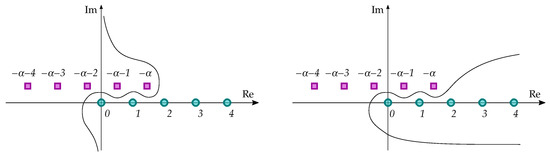
Figure 2. The curve L suitable for the Meixner weight if $b\in \mathbb{C}\backslash (0,+\infty )$ (left) and if $\left|b\right|<1$ (right).

For $\left|b\right|\ne 1$, the integral $l\left(Q\right)$ may be calculated using the Cauchy theorem. Indeed, according to (a), for $0<\left|b\right|<1$ and any $\epsilon \in (0,1/2)$, the curve L may be replaced (without changing the integral’s value) with the union of circles ${\bigcup }_{x=0}^{\infty }\{z:|z-x|=\epsilon \}$, thus giving

$$l\left(Q\right)=\frac{1}{2i}\sum _{x=0}^{\infty }{\oint }_{|z-x|=\epsilon }\frac{Q\left(z\right){(-b)}^z\Gamma (z+\alpha )}{\Gamma (z+1)sin\left(\pi z\right)}dz=\sum _{x=0}^{\infty }\frac{Q\left(x\right)b^x\Gamma (x+\alpha )}{\Gamma (x+1)}.$$

Analogously, for $\left|b\right|>1$, we obtain

$$l\left(Q\right)=-\frac{i}{2}\sum _{x=0}^{\infty }{\oint }_{|z+x+\alpha |=\epsilon }\frac{Q\left(z\right){(-b)}^z\Gamma (-z)}{\Gamma (1-z-\alpha )sin\left(\pi \right(z+\alpha \left)\right)}dz=\sum _{x=0}^{\infty }\frac{Q(-x-\alpha )b^{-x-\alpha }\Gamma (x+\alpha )}{\Gamma (x+1)},$$

which corresponds to the following relation between the Meixner polynomials:

$$M_n(-x-\alpha ;\alpha ,b^{-1})=b^n{M}_n(x;\alpha ,b)$$

stemming from the Pfaff transformation of hypergeometric functions (see ([47], p. 68) or ([39], Equation (1.4.9)).

Degenerate case $N:=-\alpha \in {\mathbb{Z}}_{⩾0}$.

Replace b by $-b$. On the one hand, the coefficients of Rodrigues’s formula for the Meixner polynomials then turn into those for the Krawtchouk polynomials—up to normalizing (correcting the sign) of odd-degree polynomials. Put in other words, the Meixner polynomials in this case reduce to the Krawtchouk polynomials, and the latter system is considered finite.

On the other hand, the Meixner weight $w\left(z\right)=w(z;\alpha ,-b)$ defined in Table 2 is infinite for $z\in \{0,\dots ,N\}$, but it can be easily regularized by a 1-periodic factor vanishing at $\mathbb{Z}$: on multiplying w by $e^{i\pi z}sin\left(\pi (z-N)\right)/\pi$ and using Euler’s reflection formula, we arrive at

$$w(z;\alpha ,-b)\frac{e^{i\pi z}sin\left(\pi (z-N)\right)}{\pi }=\frac{b^z\Gamma (z-N)sin\left(\pi (z-N)\right)}{\Gamma (z+1)\pi }=\frac{b^z}{\Gamma (z+1)\Gamma (N+1-z)},$$

and the right-hand side is exactly the Krawtchouk weight; see Table 2. Our regularization may be avoided by defining l using integration over a large enough circle:

$$l\left(Q\right)=\frac{1}{2i}{\oint }_{\left|z\right|=N+1}Q\left(z\right)w(z;-N,-b)dz\mathrm{for}Q\left(z\right)\in \mathbb{C}\left[z\right],$$

then the Cauchy integral theorem reduces the last expression to the Krawtchouk case (the circle may be replaced with other closed smooth curves separating the set $\{0,\dots ,N\}$ from infinity).

5.2. Integration Curve for Continuous Hahn Weight

The Hahn weight w is usually defined for $N\in {\mathbb{Z}}_{⩾0}$, and the corresponding measure is supported on the finite set $\{0,\dots ,N\}$. Nevertheless, general parameters are also well understood: in certain cases, the corresponding orthogonality measures turn to be discrete and finitely supported, while the generic case corresponds to a continuous weight on a complex curve.

Generic case here is $\alpha +1,\beta +1,\alpha +\beta +N+2,-N\in \mathbb{C}\backslash {\mathbb{Z}}_{⩽0}$. If so, follow [31] and choose $L=L_{\alpha ,\beta ,N}^H$ to be a smooth curve ending at $\pm i\infty$ and separating $\{-\alpha -1,-\alpha -2,\dots \}\cup \{N,N-1,\dots \}$ from $\{\beta +N+1,\beta +N+2,\dots \}\cup \{0,1,\dots \}$. Then the integral

$$\begin{array}{cc}\hfill l\left(Q\right)& :={\int }_{L}Q\left(z\right)\Gamma (z+\alpha +1)\Gamma (z-N)\Gamma (-z)\Gamma (N-z+\beta +1)dz\hfill \\ & ={\pi }^2{\int }_L\frac{Q\left(z\right)\Gamma (z+\alpha +1)\Gamma (z-N)}{\Gamma (z+1)\Gamma (z-N-\beta )sin\left(\pi z\right)sin\left(\pi \right(N-z+\beta \left)\right)}dz\hfill \end{array}$$

absolutely converges for any polynomial Q: the ratios of gamma-functions behave at infinity as powers of z, while the product of sines yields exponential decay. As is noted in Section 2.2.1 above, the degenerate case, when at least one of the numbers $\alpha +1$, $\beta +1$, $\alpha +\beta +N+2$, $-N$ is a negative integer, reduces to a discrete weight.

5.3. Properties of Raising Operators

Charlier polynomials. The raising operator for Charlier polynomials reads

$${\Psi }_k:Q\left(x\right)\mapsto -\frac{1}{w_k\left(x\right)}\nabla \left(w_k\left(x\right)Q\left(x\right)\right)=-\frac{\Gamma (x+1)}{b_k^x}\nabla \frac{b_k^{x}Q\left(x\right)}{\Gamma (x+1)}=\frac{x}{b_k}Q(x-1)-Q\left(x\right).$$

Lemma 5. 

Given a system of Charlier weights $w_1,\dots ,w_r$ as in Table 2 on ${\mathbb{Z}}_{⩾0}$, let $\mathit{n}\in {\mathbb{Z}}_{⩾0}^r$ be such that $n_k⩾1$ for some $k\in \{1,\dots ,r\}$. Suppose that the parameters of the weights $b_j\in \mathbb{C}\backslash \left\{0\right\}$ for $j=1,\dots ,r$ satisfy $b_j\ne b_k$ for all $j\ne k$. Then the conditions $Q\in {\mathcal{O}}_{\mathit{n}-{\mathit{e}}_k}$ and ${\Psi }_k\left[Q\right]\in {\mathcal{O}}_{\mathit{n}}$ are equivalent.

Proof. 

It is clear that $w_j$ is zero for $x\in {\mathbb{Z}}_{<0}$, so summation by parts yields

$$\begin{array}{c}{l}_j\left(x^m{\Psi }_k\left[Q\right]\right)=\sum _{x=0}^{\infty }{x}^m{\Psi }_k\left[Q\right]\left(x\right)·w_j\left(x\right)=-\sum _{x=0}^{\infty }{x}^m\frac{w_j\left(x\right)}{w_k\left(x\right)}\nabla \left(w_{k}Q\left(x\right)\right)\hfill \\ =\sum _{x=0}^{\infty }\nabla \left({(x+1)}^m\frac{b_j^{x+1}}{b_k^{x+1}}\right)·w_k\left(x\right)Q\left(x\right)=\sum _{x=0}^{\infty }\frac{b_j^x}{b_k^x}\left({(x+1)}^m\frac{b_j}{b_k}-x^m\right)·w_k\left(x\right)Q\left(x\right)\\ =\left(\frac{b_j}{b_k}-1\right)\sum _{x=0}^{\infty }{x}^m{w}_j\left(x\right)Q\left(x\right)+\frac{b_j}{b_k}\sum _{\nu =0}^{m-1}\left(\genfrac{}{}{0pt}{}{m}{\nu }\right)\sum _{x=0}^{\infty }{w}_j\left(x\right)Q\left(x\right)\\ \hfill =\left(\frac{b_j}{b_k}-1\right)l_j\left(x^{m}Q\right)+\frac{b_j}{b_k}\sum _{\nu =0}^{m-1}\left(\genfrac{}{}{0pt}{}{m}{\nu }\right)l_j\left(x^{\nu }Q\right).\end{array}$$

The right-hand side of this formula vanishes precisely when the left-hand side does. Since $b_j\ne b_k$ whenever $j\ne k$, we immediately obtain ${\Psi }_k\left[Q\right]\in {\mathcal{O}}_{\mathit{n}}$ if and only if $Q\in {\mathcal{O}}_{\mathit{n}-{\mathit{e}}_k}$. □

Meixner I polynomials. For the Meixner I polynomials, the raising operator has the form

$${\Psi }_k^{(\alpha ,\mathit{b})}:Q\left(x\right)\mapsto -\frac{1}{w_k^{(\alpha ,\mathit{b})}\left(x\right)}\nabla \left(w_k^{(\alpha +1,\mathit{b})}\left(x\right)Q\left(x\right)\right)=\frac{x}{b_k}Q(x-1)-(x+\alpha )Q\left(x\right).$$

Lemma 6. 

Given $N\in {\mathbb{Z}}_{>0}$ and a system of continuous Meixner weights

$${\tilde{w}}_j^{(\alpha ,\mathit{b})}\left(z\right)={(-b_j)}^z\Gamma (z+\alpha )\Gamma (-z),b_j\ne 0,\alpha \notin {\mathbb{Z}}_{⩽0},$$

on the curves $L_j=L_{b_j,\alpha }^M$ defined as above, $j=1,\dots ,r$, let there be $\mathit{n}\in {\mathbb{Z}}_{⩾0}^r$ and some $k\in \{1,\dots ,r\}$ such that $n_k⩾1$. If $b_j\ne b_k$ for all $j\ne k$, then the conditions $Q\in {\mathcal{O}}_{\mathit{n}-{\mathit{e}}_k}^{(\alpha +1,\mathit{b})}$ and ${\Psi }_k^{(\alpha ,\mathit{b})}\left[Q\right]\in {\mathcal{O}}_{\mathit{n}}^{(\alpha ,\mathit{b})}$ are equivalent (provided that ${\Psi }_k^{(\alpha ,\mathit{b})}\left[Q\right]\not\equiv 0$, which is necessarily true if $b_j\ne 1$ for all j).

Proof. 

Denote $L_j-1=\{z:z+1\in L_j\}$, then

$$\begin{array}{cc}\hfill l_j^{(\alpha ,\mathit{b})}& \left(z^m{\Psi }_k^{(\alpha ,\mathit{b})}\left[Q\right]\right)={\int }_{L_j}{z}^m\left({\frac{z}{b}}_{k}Q(z-1)-(z+\alpha )Q\left(z\right)\right){(-b_j)}^z\Gamma (z+\alpha )\Gamma (-z)dz\hfill \\ \hfill =& -{\int }_{L_j-1}{(z+1)}^{m+1}Q\left(z\right)\frac{{(-b_j)}^z{b}_j}{b_k}\Gamma (z+1+\alpha )\Gamma (-z-1)dz\hfill \\ \hfill & -{\int }_{L_j}{z}^m(z+\alpha )Q\left(z\right){(-b_j)}^z\Gamma (z+\alpha )\Gamma (-z)dz\hfill \\ \hfill =& {\int }_{L_j}\left({(z+1)}^m\frac{b_j}{b_k}-z^m\right)Q\left(z\right){(-b_j)}^z\Gamma (z+\alpha +1)\Gamma (-z)dz,\hfill \end{array}$$

where the third equality follows on replacing $L_j-1$ with $L_j$: the integration gives the same result, as both curves have similar asymptotic behavior and separate the poles of $\Gamma (z+1+\alpha )$ and $\Gamma (-z)=-(z+1)\Gamma (-1-z)$. Therefore,

$$l_j^{(\alpha ,\mathit{b})}\left(z^m{\Psi }_k^{(\alpha ,\mathit{b})}\left[Q\right]\right)=\left(\frac{b_j}{b_k}-1\right)l_j^{(\alpha +1,\mathit{b})}\left(z^{m}Q\right)+\frac{b_j}{b_k}\sum _{\nu =0}^{m-1}\left(\genfrac{}{}{0pt}{}{m}{\nu }\right)l_j^{(\alpha +1,\mathit{b})}\left(z^{\nu }Q\right).$$

The right-hand side of this formula vanishes precisely when the left-hand side does. Since $b_j\ne b_k$ whenever $j\ne k$, we immediately obtain ${\Psi }_k^{(\alpha ,\mathit{b})}\left[Q\right]\in {\mathcal{O}}_{\mathit{n}}^{(\alpha ,\mathit{b})}$ if and only if $Q\in {\mathcal{O}}_{\mathit{n}-{\mathit{e}}_k}^{(\alpha +1,\mathit{b})}$. □

Meixner II polynomials. For the Meixner II polynomials, the raising operator is given by

$$\begin{array}{cc}\hfill {\Psi }_k^{(\mathbf{\alpha },b)}:Q\left(x\right)& \mapsto -\frac{1}{w_k^{(\mathbf{\alpha },b)}\left(x\right)}\nabla \left(w_k^{(\mathbf{\alpha }+{\mathit{e}}_k,b)}\left(x\right)Q\left(x\right)\right)=-\frac{\Gamma (x+1)}{\Gamma (x+{\alpha }_k)b^x}\nabla \frac{\Gamma (x+{\alpha }_k+1)b^{x}Q\left(x\right)}{\Gamma (x+1)}\hfill \\ & =\frac{x}{b}Q(x-1)-(x+{\alpha }_k)Q\left(x\right).\hfill \end{array}$$

Lemma 7. 

Given $N\in {\mathbb{Z}}_{>0}$ and a system of continuous Meixner weights

$${\tilde{w}}_j^{(\mathbf{\alpha },b)}\left(z\right)={(-b)}^z\Gamma (z+{\alpha }_j)\Gamma (-z),b\ne 0,{\alpha }_j\notin {\mathbb{Z}}_{⩽0},$$

on the curves $L_j=L_{b,{\alpha }_j}^M$ defined as above, $j=1,\dots ,r$, let there be an index $\mathit{n}\in {\mathbb{Z}}_{⩾0}^r$ and some $k\in \{1,\dots ,r\}$ such that $n_k⩾1$. If ${\alpha }_k-{\alpha }_j\notin \{0,\dots ,n_j-1\}$ for all $j\ne k$, then the conditions $Q\in {\mathcal{O}}_{\mathit{n}-{\mathit{e}}_k}^{(\mathbf{\alpha }+{\mathit{e}}_k,b)}$ and ${\Psi }_k^{(\mathbf{\alpha },b)}\left[Q\right]\in {\mathcal{O}}_{\mathit{n}}^{(\mathbf{\alpha },b)}$ are equivalent (provided that ${\Psi }_k^{(\mathbf{\alpha },b)}\left[Q\right]\not\equiv 0$, which is necessarily true for $b\ne 1$).

If ${\alpha }_j\in {\mathbb{Z}}_{⩽0}$ for some j, then the functional $l_j$ is not quasi-definite (cf. Remark 3), and hence the whole system $l_1,\dots ,l_r$ cannot be perfect.

Proof. 

Let $m=0,\dots ,n_j-1$. Similarly to the case of the Meixner I polynomials,

$$\begin{array}{c}{l}_j^{(\mathbf{\alpha },b)}\left(z^m{\Psi }_k^{(\mathbf{\alpha },b)}\left[Q\right]\right)={\int }_{L_j}{z}^m\left(\frac{z}{b}Q(z-1)-(z+{\alpha }_k)Q\left(z\right)\right){(-b)}^z\Gamma (z+{\alpha }_j)\Gamma (-z)dz\hfill \\ =-{\int }_{L_j-1}{(z+1)}^{m+1}Q\left(z\right){(-b)}^z\Gamma (z+1+{\alpha }_j)\Gamma (-z-1)dz\\ -{\int }_{L_j}{z}^m(z+{\alpha }_k)Q\left(z\right){(-b)}^z\Gamma (z+{\alpha }_j)\Gamma (-z)dz\\ \hfill ={\int }_{L_j}\left({(z+1)}^m(z+{\alpha }_j)-z^m(z+{\alpha }_k)\right)Q\left(z\right){(-b)}^z\Gamma (z+{\alpha }_j)\Gamma (-z)dz,\end{array}$$

where the last equality follows on replacing $L_j-1$ with $L_j$. For $j=k$, the right-hand side equals

$$\sum _{\nu =0}^{m-1}\left(\genfrac{}{}{0pt}{}{m}{\nu }\right)l_k^{(\mathbf{\alpha }+{\mathit{e}}_k,b)}\left(z^{\nu }Q\right)$$

as desired. For $j\ne k$, we obtain $l_j^{(\mathbf{\alpha }+{\mathit{e}}_k,b)}=l_j^{(\mathbf{\alpha },b)}$, and hence

$$\begin{array}{cc}{l}_j^{(\mathbf{\alpha },b)}\left(z^m{\Psi }_k^{(\mathbf{\alpha },b)}\left[Q\right]\right)=\hfill & {\int }_{L_j}\left({(z+1)}^m(z+{\alpha }_j)-z^m(z+{\alpha }_k)\right)Q\left(z\right){(-b)}^z\Gamma (z+{\alpha }_j)\Gamma (-z)dz\hfill \\ & \hfill =\left({\alpha }_j-{\alpha }_k+m\right)l_j^{(\mathbf{\alpha }+{\mathit{e}}_k,b)}\left(z^{m}Q\right)+m{\alpha }_j{l}_j^{(\mathbf{\alpha }+{\mathit{e}}_k,b)}\left(z^{m-1}Q\right)+\sum _{\nu =0}^{m-2}\left(\genfrac{}{}{0pt}{}{m}{\nu }\right)l_j^{(\mathbf{\alpha }+{\mathit{e}}_k,b)}\left((z^{\nu +1}+{\alpha }_j)Q\right).\end{array}$$

(26)

The right-hand side of this formula vanishes precisely when the left-hand side does. Since ${\alpha }_k-{\alpha }_j\ne m\in \{0,\dots ,n_j-1\}$ whenever $j\ne k$, we immediately obtain ${\Psi }_k^{(\mathbf{\alpha },b)}\left[Q\right]\in {\mathcal{O}}_{\mathit{n}}^{(\mathbf{\alpha },b)}$ if and only if $Q\in {\mathcal{O}}_{\mathit{n}-{\mathit{e}}_k}^{(\mathbf{\alpha }+{\mathit{e}}_k,b)}$. □

Krawtchouk polynomials. This case may be reduced to the case of Meixner I polynomials on changing the sign of b. Nevertheless, we consider it here separately—for completeness.

$${\Psi }_{N,j}^{\left(\mathit{b}\right)}:Q\left(x\right)\mapsto -\frac{1}{w_{N,k}^{\left(\mathit{b}\right)}\left(x\right)}\nabla \left(w_{N-1,k}^{\left(\mathit{b}\right)}\left(x\right)Q\left(x\right)\right)=\frac{x}{b_k}Q(x-1)-(N-x)Q\left(x\right).$$

(27)

Lemma 8. 

Given a positive integer N and a system of Krawtchouk weights $w_{N,1}^{\left(\mathit{b}\right)}\left(x\right),\dots ,w_{N,r}^{\left(\mathit{b}\right)}\left(x\right)$, let an index $\mathit{n}\in {\{0,\dots ,N+1\}}^r$ and some $k\in \{1,\dots ,r\}$ be such that $n_k⩾1$. Suppose that $b_j\ne 0$ for $j=1,\dots ,r$, as well as $b_j\ne b_k$ for all $j\ne k$. Then the conditions $Q\in {\mathcal{O}}_{\mathit{n}-{\mathit{e}}_k}^{(\mathit{b},N-1)}$ and ${\Psi }_{N,k}^{\left(\mathit{b}\right)}\left[Q\right]\in {\mathcal{O}}_{\mathit{n}}^{(\mathit{b},N)}$ are equivalent (provided that ${\Psi }_{N,k}^{\left(\mathit{b}\right)}\left[Q\right]\not\equiv 0$, which necessarily hold true for $b\ne -1$).

Proof. 

Note that $w_{N,j}^{\left(\mathit{b}\right)}\left(x\right)$ defined in Table 2 is zero for $x\in \mathbb{Z}\backslash \{0,\dots ,N\}$, so on plugging in (27) and using summation by parts, we have

$$\begin{array}{c}{l}_{j,N}^{\left(\mathit{b}\right)}\left(x^m{\Psi }_{N,k}^{\left(\mathit{b}\right)}\left[Q\right]\right)=\sum _{x=0}^N{x}^m{\Psi }_{N,k}^{\left(\mathit{b}\right)}\left[Q\right]\left(x\right)·w_{N,j}^{\left(\mathit{b}\right)}\left(x\right)=-\sum _{x=0}^N{x}^m\frac{w_{N,j}^{\left(\mathit{b}\right)}\left(x\right)}{w_{N,k}^{\left(\mathit{b}\right)}\left(x\right)}\nabla \left(w_{N-1,k}^{\left(\mathit{b}\right)}Q\left(x\right)\right)\hfill \\ =\sum _{x=0}^{N-1}\left({(x+1)}^m\frac{b_j^{x+1}}{b_k^{x+1}}-x^m\frac{b_j^x}{b_k^x}\right)w_{N-1,k}^{\left(\mathit{b}\right)}\left(x\right)Q\left(x\right)=\sum _{x=0}^{N-1}\left({(x+1)}^m\frac{b_j}{b_k}-x^m\right)w_{N-1,j}^{\left(\mathit{b}\right)}\left(x\right)Q\left(x\right)\\ \hfill =\left(\frac{b_j}{b_k}-1\right)l_{j,N-1}^{\left(\mathit{b}\right)}\left(x^{m}Q\right)+\frac{b_j}{b_k}\sum _{\nu =0}^{m-1}\left(\genfrac{}{}{0pt}{}{m}{\nu }\right)l_{j,N-1}^{\left(\mathit{b}\right)}\left(x^{\nu }Q\right).\end{array}$$

The right-hand side of this formula vanishes precisely when the left-hand side does. Since $b_j\ne b_k$ whenever $j\ne k$, we immediately obtain ${\Psi }_{N,k}^{\left(\mathit{b}\right)}\left[Q\right]\in {\mathcal{O}}_{\mathit{n}}^{(\mathit{b},N)}$ if and only if $Q\in {\mathcal{O}}_{\mathit{n}-{\mathit{e}}_k}^{(\mathit{b},N-1)}$. □

Hahn polynomials.

The raising operator for Hahn polynomials is

$$\begin{array}{cc}\hfill {\Psi }_{N,k}^{(\mathbf{\alpha },\beta )}:Q\left(x\right)& \mapsto -\frac{1}{w_{N,k}^{(\mathbf{\alpha },\beta )}\left(x\right)}\nabla \left(w_{N-1,k}^{(\mathbf{\alpha }+{\mathit{e}}_k,\beta +1)}\left(x\right)Q\left(x\right)\right)\hfill \\ & =-\frac{\Gamma (x+1)\Gamma (N-x+1)}{{({\alpha }_k+1)}_x{(\beta +1)}_{N-x}}\nabla \frac{{({\alpha }_k+2)}_x{(\beta +2)}_{N-1-x}Q\left(x\right)}{\Gamma (x+1)\Gamma (N-x)}\hfill \\ & =\frac{x(N-x+\beta +1)Q(x-1)-(N-x)(x+{\alpha }_k+1)Q\left(x\right)}{({\alpha }_k+1)(\beta +1)}.\hfill \end{array}$$

Observe that ${\Psi }_{N,k}^{(\mathbf{\alpha },\beta )}\left[Q\right]$ is a polynomial of degree $(1+degQ)$ provided that the term ${\alpha }_k+\beta +2+degQ$ in its leading coefficient does not vanish. The constant coefficient is ${\Psi }_{N,k}^{(\mathbf{\alpha },\beta )}\left[Q\right]\left(0\right)=-NQ\left(0\right)/(\beta +1)$, so it cannot vanish unless $N=0$.

Lemma 9. 

Given $N\in {\mathbb{Z}}_{>0}$ and a system of discrete Hahn weights $w_1,\dots ,w_r$ on $\{0,1,\dots ,N\}$ such that $\beta \ne -1$ and ${\alpha }_j\ne -1$ for all j, let an index $\mathit{n}\in {\{0,\dots ,N\}}^r$ for some $k\in \{1,\dots ,r\}$ satisfy $n_k⩾1$. If ${\alpha }_k-{\alpha }_j\notin \{0,\dots ,n_j-1\}$ for all $j\ne k$ such that $n_j>0$, then

$$Q\in {\mathcal{O}}_{\mathit{n}-{\mathit{e}}_k,N-1}^{(\mathbf{\alpha }+{\mathit{e}}_k,\beta +1)}\iff {\Psi }_{N,k}^{(\mathbf{\alpha },\beta )}\left[Q\right]\in {\mathcal{O}}_{\mathit{n},N}^{(\mathbf{\alpha },\beta )}.$$

Moreover, ${\alpha }_k+\beta +2\ne -degQ$ implies $deg{\Psi }_{N,k}^{(\mathbf{\alpha },\beta )}\left[Q\right]=degQ+1$.

Proof. 

Note that $w_{N,k}^{(\mathbf{\alpha },\beta )}\left(x\right)$ is zero for $x\in \mathbb{Z}\backslash \{0,\dots ,N\}$, so for $Q\not\equiv 0$

$$\begin{array}{c}{l}_{j,N}^{(\mathbf{\alpha },\beta )}\left(x^m{\Psi }_{N,k}^{(\mathbf{\alpha },\beta )}\left[Q\right]\right)=\sum _{x=0}^N{x}^m\frac{w_{N,j}^{(\mathbf{\alpha },\beta )}\left(x\right)}{w_{N,k}^{(\mathbf{\alpha },\beta )}\left(x\right)}\nabla \left(w_{N-1,k}^{(\mathbf{\alpha }+{\mathit{e}}_k,\beta +1)}\left(x\right)Q\left(x\right)\right)\hfill \\ \hfill =\sum _{x=0}^{N-1}\nabla \left({(x+1)}^m\frac{{({\alpha }_j+1)}_{x+1}}{{({\alpha }_k+1)}_{x+1}}\right)w_{N-1,k}^{(\mathbf{\alpha }+{\mathit{e}}_k,\beta +1)}\left(x\right)Q\left(x\right),\end{array}$$

whence for $j=k$

$$l_{k,N}^{(\mathbf{\alpha },\beta )}\left(x^m{\Psi }_{N,k}^{(\mathbf{\alpha },\beta )}\left[Q\right]\right)=\sum _{\nu =0}^{m-1}\left(\genfrac{}{}{0pt}{}{m}{\nu }\right)\sum _{x=0}^{N-1}{x}^{\nu }{w}_{N-1,k}^{(\mathbf{\alpha }+{\mathit{e}}_k,\beta +1)}\left(x\right)Q\left(x\right)=\sum _{\nu =0}^{m-1}\left(\genfrac{}{}{0pt}{}{m}{\nu }\right)l_{k,N-1}^{(\mathbf{\alpha }+{\mathit{e}}_k,\beta +1)}\left(x^{\nu }Q\left(x\right)\right).$$

For $j\ne k$, we arrive at

$$\begin{array}{cc}\hfill ({\alpha }_k+1)·& l_{j,N}^{(\mathbf{\alpha },\beta )}\left(x^m{\Psi }_{N,k}^{(\mathbf{\alpha },\beta )}\left[Q\right]\right)\hfill \\ \hfill =& \sum _{x=0}^{N-1}\left({(x+1)}^m({\alpha }_j+x+1)-x^m({\alpha }_k+x+1)\right)\frac{{({\alpha }_j+1)}_x}{{({\alpha }_k+2)}_x}{w}_{N-1,k}^{(\mathbf{\alpha }+{\mathit{e}}_k,\beta +1)}\left(x\right)Q\left(x\right)\hfill \\ \hfill =& \sum _{x=0}^{N-1}\left({(x+1)}^m(x+{\alpha }_j+1)-x^m(x+{\alpha }_k+1)\right)w_{N-1,j}^{(\mathbf{\alpha }+{\mathit{e}}_k,\beta +1)}\left(x\right)Q\left(x\right)\hfill \\ \hfill =& \sum _{\nu =0}^{m-1}\left(\genfrac{}{}{0pt}{}{m}{\nu }\right)\sum _{x=0}^{N-1}{x}^{\nu }(x+{\alpha }_j+1)w_{N-1,j}^{(\mathbf{\alpha }+{\mathit{e}}_k,\beta +1)}\left(x\right)Q\left(x\right)\hfill \\ \hfill & +\left({\alpha }_j-{\alpha }_k\right)\sum _{x=0}^{N-1}{x}^m{w}_{N-1,j}^{(\mathbf{\alpha }+{\mathit{e}}_k,\beta +1)}\left(x\right)Q\left(x\right)\hfill \\ \hfill =& \left({\alpha }_j-{\alpha }_k+m\right)l_{j,N-1}^{(\mathbf{\alpha }+{\mathit{e}}_k,\beta +1)}\left(x^{m}Q\right)\hfill \\ \hfill & +m({\alpha }_j+1)l_{j,N-1}^{(\mathbf{\alpha }+{\mathit{e}}_k,\beta +1)}\left(x^{m-1}Q\right)+\sum _{\nu =0}^{m-2}\left(\genfrac{}{}{0pt}{}{m}{\nu }\right)l_{j,N-1}^{(\mathbf{\alpha }+{\mathit{e}}_k,\beta +1)}\left((x^{\nu +1}+{\alpha }_j)Q\right).\hfill \end{array}$$

Both sides of the formula are equal to zero simultaneously. Since ${\alpha }_k\ne -1$ and ${\alpha }_j-{\alpha }_k+m\ne 0$ whenever $j\ne k$, on testing $l_{j,N}^{(\mathbf{\alpha },\beta )}\left(x^m{\Psi }_{N,k}^{(\mathbf{\alpha },\beta )}\left[Q\right]\right)$ for $m=0,\dots ,n_j-1$ we immediately obtain that ${\Psi }_{N,k}^{(\mathbf{\alpha },\beta )}\left[Q\right]\in {\mathcal{O}}_{\mathit{n},N}^{(\mathbf{\alpha },\beta )}$ if and only if $Q\in {\mathcal{O}}_{\mathit{n}-{\mathit{e}}_k,N-1}^{(\mathbf{\alpha }+{\mathit{e}}_k,\beta +1)}$. □

Lemma 10. 

Given a system of continuous Hahn weights

$${\tilde{w}}_{N,j}^{(\mathbf{\alpha },\beta )}\left(z\right):=\Gamma (z+{\alpha }_j+1)\Gamma (z-N)\Gamma (-z)\Gamma (N-z+\beta +1)$$

on curves $L_j=L_{{\alpha }_j,\beta ,N}^H$, where ${\alpha }_j+1,\beta +1,{\alpha }_j+\beta +N+2,-N\in \mathbb{C}\backslash {\mathbb{Z}}_{⩽0}$, choose some $k\in \{1,\dots ,r\}$ and an index $\mathit{n}\in {\mathbb{Z}}_{⩾0}^r$ such that $n_k⩾1$. If ${\alpha }_k-{\alpha }_j\notin \{0,\dots ,n_j-1\}$ for all $j\ne k$ such that $n_j>0$, then the conditions $Q\in {\mathcal{O}}_{\mathit{n}-{\mathit{e}}_k,N-1}^{(\mathbf{\alpha }+{\mathit{e}}_k,\beta +1)}$ and ${\Psi }_{N,k}^{(\mathbf{\alpha },\beta )}\left[Q\right]\in {\mathcal{O}}_{\mathit{n},N}^{(\mathbf{\alpha },\beta )}$ are equivalent (provided that ${\Psi }_{N,k}^{(\mathbf{\alpha },\beta )}\left[Q\right]\not\equiv 0$).

Proof. 

The approach is similar to the case of multiple Meixner II polynomials. Let us remind that ${\Psi }_{N,k}^{(\mathbf{\alpha },\beta )}\left[Q\right]\not\equiv 0$, and let m run over $0,\dots ,n_j-1$.

$$\begin{array}{c}{l}_{N,j}^{(\mathbf{\alpha },\beta )}\left(z^m{\Psi }_{N,k}^{(\mathbf{\alpha },\beta )}\left[Q\right]\right)\hfill \\ ={\int }_{L_j}{z}^m\frac{z(N-z+\beta +1)Q(z-1)-(N-z)(z+{\alpha }_k+1)Q\left(z\right)}{({\alpha }_k+1)(\beta +1)}{\tilde{w}}_{N,j}^{(\mathbf{\alpha },\beta )}\left(z\right)dz\\ ={\int }_{L_j-1}{(z+1)}^{m+1}\frac{(N-z+\beta )Q\left(z\right)}{({\alpha }_k+1)(\beta +1)}{\tilde{w}}_{N,j}^{(\mathbf{\alpha },\beta )}(z+1)dz\\ -{\int }_{L_j}{z}^m\frac{(N-z)(z+{\alpha }_k+1)Q\left(z\right)}{({\alpha }_k+1)(\beta +1)}{\tilde{w}}_{N,j}^{(\mathbf{\alpha },\beta )}\left(z\right)dz\\ \hfill ={\int }_{L_j}\left({(z+1)}^m(z+{\alpha }_j+1)-z^m(z+{\alpha }_k+1)\right)Q\left(z\right)\frac{(N-z){\tilde{w}}_{N,j}^{(\mathbf{\alpha },\beta )}\left(z\right)dz}{({\alpha }_k+1)(\beta +1)},\end{array}$$

(28)

where the last equality follows by replacing $L_j-1$ with $L_j$, and then noting that

$$(z+1)(N-z+\beta ){\tilde{w}}_{N,j}^{(\mathbf{\alpha },\beta )}(z+1)=(z+{\alpha }_j+1)(N-z){\tilde{w}}_{N,j}^{(\mathbf{\alpha },\beta )}\left(z\right).$$

Replacing $L_j-1$ with $L_j$ does not change the integral’s value, as both curves have similar asymptotic behavior and separate the poles of $-\Gamma (z+{\alpha }_j+2)\Gamma (z-N+1)$ and

$$\Gamma (-z)\Gamma (N-z+\beta +1)=-(z+1)(N-z+\beta )\Gamma (-1-z)\Gamma (N-z+\beta ).$$

For $j=k$, due to $(z+{\alpha }_k+1)(N-z){\tilde{w}}_{N,k}^{(\mathbf{\alpha },\beta )}\left(z\right)=-{\tilde{w}}_{N-1,k}^{(\mathbf{\alpha }+{\mathit{e}}_k,\beta +1)}\left(z\right)$ we arrive at

$$l_{N,k}^{(\mathbf{\alpha },\beta )}\left(z^m{\Psi }_{N,k}^{(\mathbf{\alpha },\beta )}\left[Q\right]\right)=-\sum _{\nu =0}^{m-1}\left(\genfrac{}{}{0pt}{}{m}{\nu }\right)\frac{l_{N-1,k}^{(\mathbf{\alpha }+{\mathit{e}}_k,\beta +1)}\left(z^{\nu }Q\right)}{({\alpha }_k+1)(\beta +1)}$$

as required. For $j\ne k$, it follows from (28) and $(N-z){\tilde{w}}_{N,j}^{(\mathbf{\alpha },\beta )}\left(z\right)=-{\tilde{w}}_{N-1,j}^{(\mathbf{\alpha }+{\mathit{e}}_k,\beta +1)}\left(z\right)$ that

$$\begin{array}{c}-({\alpha }_k+1)(\beta +1)l_{N,j}^{(\mathbf{\alpha },\beta )}\left(z^m{\Psi }_{N,k}^{(\mathbf{\alpha },\beta )}\left[Q\right]\right)\hfill \\ ={\int }_{L_j}\left({(z+1)}^m(z+{\alpha }_j+1)-z^m(z+{\alpha }_k+1)\right)Q\left(z\right){\tilde{w}}_{N-1,j}^{(\mathbf{\alpha }+{\mathit{e}}_k,\beta +1)}\left(z\right)dz\\ =\left({\alpha }_j-{\alpha }_k+m\right)l_{N-1,j}^{(\mathbf{\alpha }+{\mathit{e}}_k,\beta +1)}\left(z^{m}Q\right)\\ \hfill +m({\alpha }_j+1)l_{N-1,j}^{(\mathbf{\alpha }+{\mathit{e}}_k,\beta +1)}\left(z^{m-1}Q\right)+\sum _{\nu =0}^{m-2}\left(\genfrac{}{}{0pt}{}{m}{\nu }\right)l_{N-1,j}^{(\mathbf{\alpha }+{\mathit{e}}_k,\beta +1)}\left((z^{\nu +1}+{\alpha }_j+1)Q\right).\end{array}$$

The right-hand side of this formula vanishes precisely when the left-hand side does. Since ${\alpha }_k-{\alpha }_j\ne m\in \{0,\dots ,n_j\}$ whenever $j\ne k$, we immediately obtain ${\Psi }_{N,k}^{(\mathbf{\alpha },\beta )}\left[Q\right]\in {\mathcal{O}}_{\mathit{n},N}^{(\mathbf{\alpha },\beta )}$ if and only if $Q\in {\mathcal{O}}_{\mathit{n}-{\mathit{e}}_k,N-1}^{(\mathbf{\alpha }+{\mathit{e}}_k,\beta +1)}$. □

Proof of Theorem 2. 

Let $\mathit{m}=(m_1,\dots ,m_r)\in {\mathbb{Z}}_{⩾0}^r$, where additionally $\left|\mathit{m}\right|⩽N$ if $N\in {\mathbb{Z}}_{⩾0}$. We apply the notation (23)–(24). For the index $\mathit{n}=(0,\dots ,0)$, the polynomial $P_{\mathit{n}}(x;\mathit{m})\equiv 1$ of degree 0 is trivially orthogonal with respect to the functionals $l_1^{\left(\mathit{m}\right)},\dots ,l_r^{\left(\mathit{m}\right)}$ stemming from the weights $w_1(x;\mathit{m}),\dots ,w_r(x;\mathit{m})$. Moreover, in the cases allowing summation over discrete weights, we have

$$l_j^{\left(\mathit{m}\right)}\left(1\right)=\left\{\begin{array}{cc}exp\left(b_j\right),\hfill & \mathrm{in}\mathrm{the}\mathrm{Charlier}\mathrm{case};\hfill \\ \Gamma (\alpha +|\mathit{m}\left|\right){(1-b_j)}^{-\alpha -\left|\mathit{m}\right|},\hfill & \mathrm{in}\mathrm{the}\mathrm{Meixner}\mathrm{I}\mathrm{case};\hfill \\ \Gamma ({\alpha }_j+m_j){(1-b)}^{-{\alpha }_j-m_j},\hfill & \mathrm{in}\mathrm{the}\mathrm{Meixner}\mathrm{II}\mathrm{case};\hfill \\ {(1+b_j)}^N/\Gamma (N-|\mathit{m}|+1),\hfill & \mathrm{in}\mathrm{the}\mathrm{Krawtchouk}\mathrm{case};\hfill \\ {\displaystyle \frac{({\alpha }_j+m_j{+\beta +\left|\mathit{m}\right|+2)}_{N-\left|\mathit{m}\right|}}{\Gamma (N-|\mathit{m}|+1)}},\hfill & \mathrm{in}\mathrm{the}\mathrm{discrete}\mathrm{Hahn}\mathrm{case},\hfill \end{array}\right.$$

(29)

where the Hahn case follows from the Chu–Vandermonde identity ([47], p. 67), ([39], Equation (1.4.3)):

$${}_2{F}_1(-N,\alpha +1;-N-\beta ;1)=\frac{{(-N-\beta -\alpha -1)}_N}{{(-N-\beta )}_N}=\frac{{(\beta +\alpha +2)}_N}{{(\beta +1)}_N}.$$

Observe that the expressions (29) for the Meixner weights remain valid (up to normalization) when we pass to parameters needing continuous weights. For the continuous Hahn weights, the expression is

$$l_j^{\left(\mathit{m}\right)}\left(1\right)={\displaystyle \frac{({\alpha }_j+m_j{+\beta +\left|\mathit{m}\right|+2)}_{N-\left|\mathit{m}\right|}\Gamma ({\alpha }_j+m_j+1)\Gamma (\beta +|\mathit{m}|+1)}{{(-1)}^{\left|\mathit{m}\right|+1}2\Gamma (N-|\mathit{m}|+1)sin\left(\pi N\right)}},$$

(30)

see ([31], Equation (4)). As a result, $l_j^{\left(\mathit{m}\right)}\left(1\right)\notin \{0,\infty \}$ under the conditions (i)–(v) of Theorem 2.

Using this fact as a base, we now apply induction in $M\in {\mathbb{Z}}_{⩾0}$. Put $\tilde{N}:=N$ if $N\in {\mathbb{Z}}_{⩾0}$, and $\tilde{N}:=\infty$ otherwise. Given M, for all shifts $\mathit{m}\in {\mathbb{Z}}_{⩾0}^r$ satisfying $\left|\mathit{m}\right|⩽\tilde{N}$ and for all indices $\mathit{n}$ satisfying $\left|\mathit{n}\right|⩽min(\tilde{N}-|\mathit{m}|,M-1)$, let $P_{\mathit{n}}(x;\mathit{m})\in {\mathcal{O}}_{\mathit{n}}^{\left(\mathit{m}\right)}\backslash {\bigcup }_{k=1}^r{\mathcal{O}}_{\mathit{n}+{\mathit{e}}_k}^{\left(\mathit{m}\right)}$ be the unique polynomial of degree $\left|\mathit{n}\right|$ constructed via Rodrigues’s Formula (25). Let us show that the same holds for $\mathit{n}$ satisfying $\left|\mathit{n}\right|=M⩽\tilde{N}-\left|\mathit{m}\right|$. Indeed, by Lemma 4, the polynomials

$$P_{\mathit{n}}(x;\mathit{m})={\Psi }_j^{\left(\mathit{m}\right)}\left[P_{\mathit{n}-{\mathit{e}}_j}(x;\mathit{m}+{\mathit{e}}_j)\right]$$

do not depend on j such that $n_j>0$. Since $|\mathit{n}-{\mathit{e}}_j|=M-1⩽\tilde{N}-|\mathit{m}+{\mathit{e}}_j|$, we have $P_{\mathit{n}-{\mathit{e}}_j}(x;\mathit{m}+{\mathit{e}}_j)\in {\mathcal{O}}_{\mathit{n}-{\mathit{e}}_j}^{(\mathit{m}+{\mathit{e}}_j)}\backslash {\bigcup }_{k=1}^r{\mathcal{O}}_{\mathit{n}-{\mathit{e}}_j+{\mathit{e}}_k}^{(\mathit{m}+{\mathit{e}}_j)}$. Therefore, Lemmas 5–9 imply that $P_{\mathit{n}}(x;\mathit{m})\in {\mathcal{O}}_{\mathit{n}}^{\left(\mathit{m}\right)}\backslash {\bigcup }_{k=1}^r{\mathcal{O}}_{\mathit{n}+{\mathit{e}}_k}^{\left(\mathit{m}\right)}$. Moreover, under the theorem’s conditions (i)–(v), each of the raising operators increases the degree of polynomials by 1, and thus $deg{P}_{\mathit{n}}(x;\mathit{m})=\left|\mathit{n}\right|$. So, Lemma 2 furnishes the proof of the “if” assertion of the theorem.

The “only if” assertion follows on noting that if the relevant condition of Theorem 2 fails to hold, then there is an index $\mathit{n}$ that is not normal. Indeed, either the raising operator does not increase degrees of polynomials, or $l_j^{\left(\mathit{m}\right)}\left(1\right)\in \{0,\infty \}$ for some $\mathit{m}$ and j, which is seen from (29) and (30).

More specifically, for the Charlier, Meixner and Krawtchouk weights, the condition $b\ne 0$ or $b_j\ne 0$ means that the jth weight is not zero identically, which is already required for the normality of the index ${\mathit{e}}_j$.

Now, let $b_j=1$ in the Krawtchouk case; then the corresponding raising operator does not increase the degree of polynomials, and unless $N=0$, the polynomial $Q\left(x\right)\equiv 1$ turns to be orthogonal to all monomials by Lemma 8, meaning absence of normality for $\mathit{n}\ne (0,\dots ,0)$. If $N\in {\mathbb{Z}}_{⩾0}$, the Krawtchouk weights are supported on $N+1$ points, so the polynomial ${(x-N)}_{N+1}$ is orthogonal to all monomials; thus, the normality of $\mathit{n}$ is only possible if $\left|\mathit{n}\right|⩽N+1$. Moreover, the condition $b_j\ne b_k$ is required by normality when $\left|\mathit{n}\right|⩾2$.

The case of the Meixner I system is similar to the Krawtchouk case: we only have to replace $b_j\to -b_j$ and $\alpha \to -N$. For $\alpha \in {\mathbb{Z}}_{⩽0}$, the Meixner functionals $l_j$ should be replaced by their regularization—that is by the Krawtchouk functionals.

The “only if” assertion of Theorem 2 for the Meixner II system may be dealt analogously. The main difference here is seen from (26): if ${\alpha }_j+m={\alpha }_k$, then Lemma 2 implies the absence of normality for the orthogonal polynomial $P_{m{\mathit{e}}_k}\in {\mathcal{O}}_{{\mathit{e}}_j+m{\mathit{e}}_k}^{(\mathbf{\alpha },b)}$ produced by iterations of the raising operator.

For the Hahn polynomials, if ${\alpha }_k$ or $\beta \in {\mathbb{Z}}_{<0}$, then in Theorem 2, we have $N\in {\mathbb{Z}}_{⩾0}$. In this case, if ${\alpha }_k\in \{-1,\dots ,1-N\}$ for some k and $\beta \in \mathbb{C}\backslash \{-1,\dots ,{\alpha }_k\}$, then

$$l_k\left(x^m·{(x+{\alpha }_k+1)}_{-{\alpha }_k}\right)=0$$

for all $m\in {\mathbb{Z}}_{⩾0}$ yielding the absence of normality of the corresponding indices (i.e., the indices $n_k{\mathit{e}}_k$ with $n_k>-{\alpha }_k$ are not normal). Analogously, if $\beta \in \{-1,\dots ,1-N\}$, then ${(N-x+\beta +1)}_{-\beta }\in O_{\mathit{n},N}^{(\mathbf{\alpha },\beta )}$ for all indices $\mathit{n}$, and hence, there is no normality for $\left|\mathit{n}\right|>-\beta$.

If $N\in \mathbb{C}\backslash {\mathbb{Z}}_{⩾0}$, then ${\Psi }_{N,k}^{(\mathbf{\alpha },\beta )}\left[Q\right]$ is a polynomial of degree $degQ+1$ if and only if ${\alpha }_k+\beta +2+degQ\ne 0$. So when ${\alpha }_k+\beta +2+\left|\mathit{n}\right|=0$ for some index $\mathit{n}$, we still obtain an orthogonal polynomial $P_{\mathit{n}+{\mathit{e}}_k}\not\equiv 0$ by iterations of the raising operator, while $deg{P}_{\mathit{n}+{\mathit{e}}_k}<\left|\mathit{n}\right|+1$ implies absence of normality of $\mathit{n}+{\mathit{e}}_k$. As is seen from (29) and (30), such a situation cannot occur under the condition that $l_j^{\left(\mathit{m}\right)}\left(1\right)\ne 0$ for all j and $\mathit{m}$. When $N\in {\mathbb{Z}}_{>0}$ and ${\alpha }_k,\beta \in \mathbb{C}\backslash \{-1,\dots ,1-N\}$ for all k, one tests this condition for $\left|\mathit{m}\right|⩽N$ to verify the normality of all indices $\mathit{n}$ satisfying $\left|\mathit{n}\right|⩽N$. (For the index ${\mathit{e}}_k$ when ${\alpha }_k+\beta \ne -2$ but ${\alpha }_k=-1$ or $\beta =-1$, the orthogonal polynomials are given by the regularization: respectively, $(1+{\alpha }_k){\Psi }_{N,k}^{(\mathbf{\alpha },\beta )}\left[1\right]=x$ or $(1+\beta ){\Psi }_{N,k}^{(\mathbf{\alpha },\beta )}\left[1\right]=x-N$.) □

References

- Hermite, C. Sur la fonction exponentielle. C. R. Acad. Sci. Paris Sér. I Math. 1873, 77, 18–24, 74–79, 226–233, 285–293. [Google Scholar]
- Van Assche, W. Multiple orthogonal polynomials, irrationality and transcendence. In Continued Fractions: From Analytic Number Theory to Constructive Approximation; Berndt, B.C., Gesztesy, F., Eds.; American Mathematical Society: Providence, RI, USA, 1999; Volume 236, pp. 325–342. [Google Scholar]
- Sorokin, V.N. Cyclic graphs and Apéry’s theorem. Russ. Math. Surv. 2002, 57, 535–571. [Google Scholar] [CrossRef]
- Sorokin, V.N. On Salikhov’s integral. Trans. Moscow Math. Soc. 2016, 77, 107–126. [Google Scholar] [CrossRef]
- Marcovecchio, R. Vectors of type II Hermite-Padé approximations and a new linear independence criterion. Ann. Mat. Pura Appl. 2021, 200, 2829–2861. [Google Scholar] [CrossRef]
- Kuijlaars, A.B.J. Multiple orthogonal polynomial ensembles. In Recent Trends in Orthogonal Polynomials and Approximation Theory; American Mathematical Society: Providence, RI, USA, 2010; Volume 507, pp. 155–176. [Google Scholar]
- Aptekarev, A.I.; Denisov, S.A.; Yattselev, M.L. Self-adjoint Jacobi matrices on trees and multiple orthogonal polynomials. Trans. Am. Math. Soc. 2020, 373, 875–917. [Google Scholar] [CrossRef]
- Doliwa, A. Non-commutative Hermite-Padé approximation and integrability. Lett. Math. Phys. 2022, 112, 17. [Google Scholar] [CrossRef]
- Mahler, K. Perfect systems. Compos. Math. 1968, 19, 95–166. [Google Scholar]
- Chihara, T.S. An Introduction to Orthogonal Polynomials. Mathematics and Its Applications; Gordon and Breach Science Publishers: New York, NY, USA; London, UK; Paris, France, 1978; Volume 13. [Google Scholar]
- Nikishin, E.M.; Sorokin, V.N. Rational approximations and orthogonality. In Translations of Mathematical Monographs; Boas, R.P., Translator; American Mathematical Society: Providence, RI, USA, 1991; Volume 92, pp. viii+221. [Google Scholar]
- Coussement, J.; Van Assche, W. Gaussian quadrature for multiple orthogonal polynomials. J. Comput. Appl. Math. 2005, 178, 131–145. [Google Scholar] [CrossRef]
- Milovanović, G.V. Generalized weighted Birkhoff-Young quadratures with the maximal degree of exactness. Appl. Numer. Math. 2017, 116, 238–255. [Google Scholar] [CrossRef]
- Jovanović, A.N.; Stanić, M.P.; Tomović, T.V. Construction of the optimal set of quadrature rules in the sense of Borges. Electron. Trans. Numer. Anal. 2018, 50, 164–181. [Google Scholar] [CrossRef]
- Nikiforov, A.F.; Uvarov, V.B. Special Functions of Mathematical Physics; A Unified Introduction with Applications; Boas, R.P., Samarskiĭ, A.A., Translators; Birkhäuser: Basel, Switzerland, 1988; pp. xviii+427. [Google Scholar]
- Van Assche, W.; Coussement, E. Some classical multiple orthogonal polynomials. J. Comput. Appl. Math. 2001, 127, 317–347. [Google Scholar] [CrossRef]
- Aptekarev, A.I.; Branquinho, A.; Van Assche, W. Multiple orthogonal polynomials for classical weights. Trans. Am. Math. Soc. 2003, 355, 3887–3914. [Google Scholar] [CrossRef]
- Aptekarev, A.I.; Bleher, P.M.; Kuijlaars, A.B.J. Large n limit of Gaussian random matrices with external source. II. Commun. Math. Phys. 2005, 259, 367–389. [Google Scholar]
- Bleher, P.M.; Kuijlaars, A.B.J. Random matrices with external source and multiple orthogonal polynomials. Int. Math. Res. Not. 2004, 2004, 109–129. [Google Scholar] [CrossRef]
- Desrosiers, P.; Forrester, P.J. Asymptotic correlations for Gaussian and Wishart matrices with external source. Int. Math. Res. Not. 2006, 2006, 27395. [Google Scholar] [CrossRef]
- Piñeiro Días, L.R. On simultaneous approximations for some collection of Markov functions. Vestn. Moskov. Univ. Ser. I Mat. Mekh. 1987, 1987, 67–70. [Google Scholar]
- Adler, M.; van Moerbeke, P.; Wang, D. Random matrix minor processes related to percolation theory. Random Matrices Theory Appl. 2013, 2, 1350008. [Google Scholar] [CrossRef]
- Marcellán, F.; Rocha, I.A. Complex path integral representation for semiclassical linear functionals. J. Approx. Theory 1998, 94, 107–127. [Google Scholar]
- Kuijlaars, A.B.J.; Martinez-Finkelshtein, A.; Orive, R. Orthogonality of Jacobi polynomials with general parameters. Electron. Trans. Numer. Anal. 2005, 19, 1–17. [Google Scholar]
- Kuijlaars, A.B.J.; McLaughlin, K.T.R. Asymptotic zero behavior of Laguerre polynomials with negative parameter. Constr. Approx. 2004, 20, 497–523. [Google Scholar] [CrossRef]
- Kuijlaars, A.B.J.; Martínez-Finkelshtein, A. Strong asymptotics for Jacobi polynomials with varying nonstandard parameters. J. Anal. Math. 2004, 94, 195–234. [Google Scholar] [CrossRef]
- Mukhin, E.; Varchenko, A. Multiple orthogonal polynomials and a counterexample to the Gaudin Bethe Ansatz Conjecture. Trans. Am. Math. Soc. 2007, 359, 5383–5418. [Google Scholar] [CrossRef]
- Beckermann, B.; Coussement, J.; Van Assche, W. Multiple Wilson and Jacobi-Piñeiro polynomials. J. Approx. Theory 2005, 132, 155–181. [Google Scholar] [CrossRef]
- Nikiforov, A.F.; Suslov, S.K.; Uvarov, V.B. Classical Orthogonal Polynomials of a Discrete Variable; Springer Series in Computational Physics; Translated from the Russian; Springer: Berlin, Germany, 1991; pp. xvi+374. [Google Scholar]
- Atakishiyev, N.M.; Suslov, S.K. The Hahn and Meixner polynomials of an imaginary argument and some of their applications. J. Phys. A 1985, 18, 1583–1596. [Google Scholar] [CrossRef]
- Askey, R. Continuous Hahn polynomials. J. Phys. A 1985, 18, L1017–L1019. [Google Scholar] [CrossRef]
- Baik, J.; Kriecherbauer, T.; McLaughlin, K.T.R.; Miller, P.D. Discrete Orthogonal Polynomials; Annals of Mathematics Studies; Asymptotics and Applications; Princeton University Press: Princeton, NJ, USA, 2007; Volume 164, pp. viii+170. [Google Scholar]
- Aversú, J.; Coussement, E.; Van Assche, W. Some discrete multiple orthogonal polynomials. J. Comput. Appl. Math. 2003, 153, 19–45. [Google Scholar]
- Vinet, L.; Zhedanov, A. Automorphisms of the Heisenberg-Weyl algebra and d-orthogonal polynomials. J. Math. Phys. 2009, 50, 033511. [Google Scholar] [CrossRef]
- Prévost, M.; Rivoal, T. Remainder Padé approximants for the exponential function. Constr. Approx. 2007, 25, 109–123. [Google Scholar] [CrossRef]
- Miki, H.; Tsujimoto, S.; Vinet, L.; Zhedanov, A. An algebraic model for the multiple Meixner polynomials of the first kind. J. Phys. A 2012, 45, 325205. [Google Scholar] [CrossRef]
- Ndayiragije, F.; Van Assche, W. Multiple Meixner polynomials and non-Hermitian oscillator Hamiltonians. J. Phys. A 2013, 46, 505201. [Google Scholar] [CrossRef]
- Bender, M.; Delvaux, S.; Kuijlaars, A.B.J. Multiple Meixner-Pollaczek polynomials and the six-vertex model. J. Approx. Theory 2011, 163, 1606–1637. [Google Scholar]
- Ismail, M.E.H. Classical and Quantum Orthogonal Polynomials in One Variable; Encyclopedia of Mathematics and Its Applications; Cambridge University Press: Cambridge, UK, 2005. [Google Scholar] [CrossRef]
- Van Assche, W. Nearest neighbor recurrence relations for multiple orthogonal polynomials. J. Approx. Theory 2011, 163, 1427–1448. [Google Scholar] [CrossRef]
- Aptekarev, A.I.; Derevyagin, M.; Van Assche, W. Discrete integrable systems generated by Hermite-Padé approximants. Nonlinearity 2016, 29, 1487–1506. [Google Scholar] [CrossRef]
- Aptekarev, A.I.; Derevyagin, M.; Miki, H.; Van Assche, W. Multidimensional Toda lattices: Continuous and discrete time. SIGMA Symmetry Integr. Geom. Methods Appl. 2016, 12, 30. [Google Scholar] [CrossRef]
- Aptekarev, A.I.; Lysov, V.G. Multilevel interpolation for Nikishin systems and boundedness of Jacobi matrices on binary trees. Russ. Math. Surv. 2021, 76, 726–728. [Google Scholar] [CrossRef]
- Denisov, S.A.; Yattselev, M.L. Spectral theory of Jacobi matrices on trees whose coefficients are generated by multiple orthogonality. Adv. Math. 2022, 396, 108114. [Google Scholar] [CrossRef]
- Aptekarev, A.I.; Kalyagin, V.; López Lagomasino, G.; Rocha, I.A. On the limit behavior of recurrence coefficients for multiple orthogonal polynomials. J. Approx. Theory 2006, 139, 346–370. [Google Scholar] [CrossRef]
- Erdélyi, A.; Magnus, W.; Oberhettinger, F.; Tricomi, F.G. Higher Transcendental Functions; Bateman Manuscript Project; McGraw-Hill Book Co.: New York, NY, USA, 1953; Volume I. [Google Scholar]
- Andrews, G.E.; Askey, R.; Roy, R. Special Functions; Encyclopedia of Mathematics and Its Applications; Cambridge University Press: Cambridge, UK, 1999; Volume 71. [Google Scholar]
- Alfaro, M.; Pérez, T.E.; Piñar, M.A.; Rezola, M.L. Sobolev orthogonal polynomials: The discrete-continuous case. Meth. Appl. Anal. 1999, 6, 593–616. [Google Scholar] [CrossRef]
- Alfaro, M.; de Morales, M.A.; Rezola, M.L. Orthogonality of the Jacobi polynomials with negative integer parameters. J. Comput. Appl. Math. 2002, 145, 379–386. [Google Scholar] [CrossRef]
- Costas-Santos, R.; Sánchez-Lara, J. Extensions of discrete classical orthogonal polynomials beyond the orthogonality. J. Comput. Appl. Math. 2009, 225, 440–451. [Google Scholar] [CrossRef]
Disclaimer/Publisher’s Note: The statements, opinions and data contained in all publications are solely those of the individual author(s) and contributor(s) and not of MDPI and/or the editor(s). MDPI and/or the editor(s) disclaim responsibility for any injury to people or property resulting from any ideas, methods, instructions or products referred to in the content. |
© 2023 by the authors. Licensee MDPI, Basel, Switzerland. This article is an open access article distributed under the terms and conditions of the Creative Commons Attribution (CC BY) license (https://creativecommons.org/licenses/by/4.0/).