Non-Resonant Non-Hyperbolic Singularly Perturbed Neumann Problem

Abstract

In this brief note, we study the problem of asymptotic behavior of the solutions for non-resonant, singularly perturbed linear Neumann boundary value problems $\epsilon y^{″}+ky=f\left(t\right)$, $y^{\prime }\left(a\right)=0$, $y^{\prime }\left(b\right)=0$, $k>0,$ with an indication of possible extension to more complex cases. Our approach is based on the analysis of an integral equation associated with this problem.

1. Introduction

In this paper, we are dealing with the singularly perturbed linear problem

$$\epsilon y^{″}+ky=f\left(t\right),k>0,0<\epsilon \ll 1,f\in C^3\left([a,b]\right),$$

(1)

with the Neumann boundary condition

$$y^{\prime }\left(a\right)=0,y^{\prime }\left(b\right)=0.$$

(2)

The analysis of the differential equations under consideration is complicated by the fact that all roots of characteristic equations of this differential equation are located on the imaginary axis; that is, the differential equation is not hyperbolic. For the singularly perturbed dynamical systems, the dynamics near a normally hyperbolic critical manifold are well-known; see [1,2,3,4,5] for a geometric approach to the singular perturbation theory, Refs. [6,7,8,9] for the lower and upper solution method and [10] for applications in control theory. However, if the condition of normal hyperbolicity of a critical manifold is not fulfilled, then the problem of existence and asymptotic behavior (as $\epsilon \to 0^{+}$) of solutions is hard to solve in general, and leads to the principal technical difficulties in nonlinear cases; see, for example [11]. Thus, the considerations below may be instructive and helpful for the analyses of this class of problems. The calculations that will follow (and thus, the main result formulated in Theorem 1 below) can also be applied to nonlinear differential equations, where the right-hand side of (1), (2) will have the function $f(t,y)$ instead of $f\left(t\right),$ but in this case it will be necessary to guarantee that the set of solutions $y_{\epsilon }\left(t\right),$$\epsilon \to 0^{+},$ of such problems also belong to the space $C^3\left([a,b]\right)$, and are uniformly bounded together with their second and third derivatives on the interval $[a,b]$ (Remark 2). The uniform boundedness of the first derivatives follows from the boundary conditions imposed on the solutions (2), and uniform boundedness of the second derivatives.

Despite these difficulties, we will prove that there are an infinite number of sequences ${\left\{{\epsilon }_n\right\}}_{n=0}^{\infty },$${\epsilon }_n\to 0^{+}$, such that $y_{{\epsilon }_n}\left(t\right)$ converge uniformly to $u\left(t\right)$ on $[a,b]$ for ${\epsilon }_n\to 0^{+},$ where $y_{{\epsilon }_n}$ is a solution of the Problem (1), (2) with $\epsilon ={\epsilon }_n$ and u represents the critical manifold for our system, that is, a solution of the reduced problem $ky=f\left(t\right)$ obtained from Equation (1) for $\epsilon =0.$

Henceforth, in this paper, for the values of parameter $\epsilon$, we consider the closed intervals $J_n$ only, defined as

$$J_n\triangleq \left[k{\left(\frac{b-a}{(n+1)\pi -\lambda }\right)}^2,k{\left(\frac{b-a}{n\pi +\lambda }\right)}^2\right],n=0,1,2,\cdots ,$$

where $\lambda >0$ is an arbitrarily small but fixed constant ($\lambda \ll \pi /2$), which guarantees the existence and uniqueness to the solutions of (1), (2); that is, a non-resonant case.

Example 1.

As an academic example, let us consider the linear problem

$$\epsilon y^{″}+ky=e^t,t\in [a,b],k>0,0<\epsilon \ll 1,$$

$$y^{\prime }\left(a\right)=0,y^{\prime }\left(b\right)=0,$$

and its solution

$$y_{\epsilon }\left(t\right)=\frac{-e^{a}cos\left[\sqrt{\frac{k}{\epsilon }}(b-t)\right]+e^{b}cos\left[\sqrt{\frac{k}{\epsilon }}(t-a)\right]}{\sqrt{\frac{k}{\epsilon }}(k+\epsilon )sin\left[\sqrt{\frac{k}{\epsilon }}(b-a)\right]}+\frac{e^t}{k+\epsilon }.$$

Hence, for every sequence ${\left\{{\epsilon }_n\right\}}_{n=0}^{\infty }$, ${\epsilon }_n\in J_n,$ the solution of the problem under consideration satisfies

$$y_{{\epsilon }_n}\left(t\right)=\frac{e^t}{k+{\epsilon }_n}+O\left({\sqrt{\epsilon }}_n\right)$$

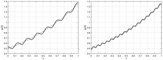
and thus, the solutions converge uniformly on the interval $[a,b]$ to the solution $u\left(t\right)=e^t/k$ of the reduced problem for $n\to \infty .$ The second term on the right-hand side denotes the convenient Big–O notation. For better illustration, Figure 1 graphically shows the solutions for different values of the parameter $\epsilon .$ The MATLAB code for Figure 1 is below, in Listing 1.

Figure 1. Solutions of the Neumann boundary value problem from Example 1 on the interval $[0,1]$ for $k=2$ and $\epsilon =0.001$ (left) and $\epsilon =0.0002$ (right). A dashed line is used to draw the function $u\left(t\right)=e^t/k,$ the solution of the reduced problem.

Listing 1. MATLAB code for Figure 1.

%bvp5cNeumann.m

format long;

a = 0;

b = 1;

k = 2;

eps = 0.0002;

ode = @(x,y) [y(2) ; (-k*y(1) + exp(x))/eps];

bc = @(ya,yb)[ya(2); yb(2)]; %Neumann BC

solinit = bvpinit(linspace(a,b,50),[1 0]);

sol = bvp5c(ode,bc,solinit);

x = linspace(a,b);

y = deval(sol,x);

X=x’; Y=y(1,:)’;

%[X Y]

plot(x,Y,’linewidth’,1.5);

hold on

plot(x,exp(x)/k, ’--’);

hold on

grid on

xlabel(’$t$’,’interpreter’,’latex’);

ylabel(’$y_{\varepsilon}(t)$’,’interpreter’,’latex’);

%print(’figure1’,’-deps’)

The main result of this note is the following theorem generalizing the Example 1 to all right-hand sides $f\left(t\right).$

2. Main Result

Theorem 1.

For all $f\in C^3\left([a,b]\right)$ and for every sequence ${\left\{{\epsilon }_n\right\}}_{n=0}^{\infty }$, ${\epsilon }_n\in J_n$ there exists a unique sequence of the solutions ${\left\{y_{{\epsilon }_n}\right\}}_{n=0}^{\infty }$ of the Problem (1), (2) satisfying

$$y_{{\epsilon }_n}\to u\mathrm{uniformly}\mathrm{on}[a,b]\mathrm{for}n\to \infty .$$

More precisely,

$$y_{{\epsilon }_n}\left(t\right)=\frac{f\left(t\right)}{k}+O\left(\sqrt{{\epsilon }_n}\right)\mathrm{on}[a,b]$$

for $n\to \infty$ ($\Rightarrow {\epsilon }_n\to 0^{+}$) and, if $f^{\prime }\left(a\right)=f^{\prime }\left(b\right)=0$, then on $[a,b]$, the following asymptotics for $n\to \infty$ hold:

$$y_{{\epsilon }_n}\left(t\right)=\frac{f\left(t\right)}{k}+O\left({\epsilon }_n\right)\mathrm{and}{y}_{{\epsilon }_n}^{\prime }\left(t\right)=\frac{f^{\prime }\left(t\right)}{k}+O\left(\sqrt{{\epsilon }_n}\right).$$

Proof. 

First, we show that the function

$$\begin{array}{ccc}\hfill y_{\epsilon }\left(t\right)& =& \frac{cos\left[\sqrt{\frac{k}{\epsilon }}(t-a)\right]\underset{a}{\overset{b}{\int }}cos\left[\sqrt{\frac{k}{\epsilon }}(b-s)\right]\frac{f\left(s\right)}{\epsilon }\mathrm{d}s}{\sqrt{\frac{k}{\epsilon }}sin\left[\sqrt{\frac{k}{\epsilon }}(b-a)\right]}\hfill \\ & +& \underset{a}{\overset{t}{\int }}\frac{sin\left[\sqrt{\frac{k}{\epsilon }}(t-s)\right]\frac{f\left(s\right)}{\epsilon }}{\sqrt{\frac{k}{\epsilon }}}\mathrm{d}s\hfill \end{array}$$

(3)

is a solution of (1), (2). Differentiating (3) twice, taking into consideration the relation

$$\frac{\mathrm{d}}{\mathrm{d}t}\underset{a}{\overset{t}{\int }}H(t,s)f\left(s\right)\mathrm{d}s=\underset{a}{\overset{t}{\int }}\frac{\partial H(t,s)}{\partial t}f\left(s\right)\mathrm{d}s+H(t,t)f\left(t\right),$$

we obtain that

$$\begin{array}{ccc}\hfill y_{\epsilon }^{\prime }\left(t\right)& =& -\frac{\sqrt{\frac{k}{\epsilon }}sin\left[\sqrt{\frac{k}{\epsilon }}(t-a)\right]\underset{a}{\overset{b}{\int }}cos\left[\sqrt{\frac{k}{\epsilon }}(b-s)\right]\frac{f\left(s\right)}{\epsilon }\mathrm{d}s}{\sqrt{\frac{k}{\epsilon }}sin\left[\sqrt{\frac{k}{\epsilon }}(b-a)\right]}\hfill \end{array}$$

$$\begin{array}{ccc}& +& \underset{a}{\overset{t}{\int }}\frac{\sqrt{\frac{k}{\epsilon }}cos\left[\sqrt{\frac{k}{\epsilon }}(t-s)\right]\frac{f\left(s\right)}{\epsilon }}{\sqrt{\frac{k}{\epsilon }}}\mathrm{d}s,\hfill \\ \hfill y_{\epsilon }^{″}\left(t\right)& =& -\frac{{\left(\sqrt{\frac{k}{\epsilon }}\right)}^{2}cos\left[\sqrt{\frac{k}{\epsilon }}(t-a)\right]\underset{a}{\overset{b}{\int }}cos\left[\sqrt{\frac{k}{\epsilon }}(b-s)\right]\frac{f\left(s\right)}{\epsilon }\mathrm{d}s}{\sqrt{\frac{k}{\epsilon }}sin\left[\sqrt{\frac{k}{\epsilon }}(b-a)\right]}\hfill \end{array}$$

(4)

$$\begin{array}{ccc}& -& \underset{a}{\overset{t}{\int }}\frac{{\left(\sqrt{\frac{k}{\epsilon }}\right)}^{2}sin\left[\sqrt{\frac{k}{\epsilon }}(t-s)\right]\frac{f\left(s\right)}{\epsilon }}{\sqrt{\frac{k}{\epsilon }}}\mathrm{d}s+\frac{f\left(t\right)}{\epsilon }.\hfill \end{array}$$

(5)

From (5) and (3), after a little algebraic rearrangement, we get

$$y_{\epsilon }^{″}=\frac{k}{\epsilon }\left(-y_{\epsilon }\right)+\frac{f\left(t\right)}{\epsilon },$$

that is, $y_{\epsilon }$ is a solution of differential Equation (1), and from (4), it is easy to verify that this solution of (1) satisfies the boundary condition (2).

Let $t_0\in [a,b]$ be arbitrary, but fixed. Let us denote by $I_1$ and $I_2$ the integrals

$$I_1\triangleq \underset{a}{\overset{b}{\int }}cos\left[\sqrt{\frac{k}{\epsilon }}(b-s)\right]\frac{f\left(s\right)}{\epsilon }\mathrm{d}s$$

and

$$I_2\triangleq \underset{a}{\overset{t_0}{\int }}sin\left[\sqrt{\frac{k}{\epsilon }}\left(t_0-s\right)\right]\frac{f\left(s\right)}{\epsilon }\mathrm{d}s.$$

Then

$$y_{\epsilon }\left(t_0\right)=\frac{cos\left[\sqrt{\frac{k}{\epsilon }}\left(t_0-a\right)\right]I_1}{\sqrt{\frac{k}{\epsilon }}sin\left[\sqrt{\frac{k}{\epsilon }}(b-a)\right]}+\frac{I_2}{\sqrt{\frac{k}{\epsilon }}}.$$

Integrating $I_1$ and $I_2$ by parts we obtain that

$$\begin{array}{ccc}\hfill I_1& =& \sqrt{\frac{\epsilon }{k}}sin\left[\sqrt{\frac{k}{\epsilon }}(b-a)\right]\frac{f\left(a\right)}{\epsilon }+\underset{a}{\overset{b}{\int }}\sqrt{\frac{\epsilon }{k}}sin\left[\sqrt{\frac{k}{\epsilon }}(b-s)\right]\frac{f^{\prime }\left(s\right)}{\epsilon }\mathrm{d}s,\hfill \\ \hfill I_2& =& \frac{\sqrt{\frac{\epsilon }{k}}f\left(t_0\right)}{\epsilon }-\sqrt{\frac{\epsilon }{k}}cos\left[\sqrt{\frac{k}{\epsilon }}\left(t_0-a\right)\right]\frac{f\left(a\right)}{\epsilon }-\underset{a}{\overset{t_0}{\int }}\sqrt{\frac{\epsilon }{k}}cos\left[\sqrt{\frac{k}{\epsilon }}\left(t_0-s\right)\right]\frac{f^{\prime }\left(s\right)}{\epsilon }\mathrm{d}s.\hfill \end{array}$$

Thus,

$$\begin{array}{ccc}\hfill y_{\epsilon }\left(t_0\right)& =& \frac{f\left(t_0\right)}{k}+\frac{cos\left[\sqrt{\frac{k}{\epsilon }}\left(t_0-a\right)\right]}{sin\left[\sqrt{\frac{k}{\epsilon }}(b-a)\right]}\underset{a}{\overset{b}{\int }}sin\left[\sqrt{\frac{k}{\epsilon }}(b-s)\right]\frac{f^{\prime }\left(s\right)}{k}\mathrm{d}s\hfill \\ & -& \underset{a}{\overset{t_0}{\int }}cos\left[\sqrt{\frac{k}{\epsilon }}\left(t_0-s\right)\right]\frac{f^{\prime }\left(s\right)}{k}\mathrm{d}s.\hfill \end{array}$$

Now, we estimate the difference $y_{\epsilon }\left(t_0\right)-\frac{f\left(t_0\right)}{k}.$ We have

$$\begin{array}{ccc}\hfill \left|y_{\epsilon }\left(t_0\right)-\frac{f\left(t_0\right)}{k}\right|& \le & \frac{1}{ksin\lambda }\left|\underset{a}{\overset{b}{\int }}sin\left[\sqrt{\frac{k}{\epsilon }}(b-s)\right]f^{\prime }\left(s\right)\mathrm{d}s\right|\hfill \\ & +& \frac{1}{k}\left|\underset{a}{\overset{t_0}{\int }}cos\left[\sqrt{\frac{k}{\epsilon }}\left(t_0-s\right)\right]f^{\prime }\left(s\right)\mathrm{d}s\right|.\hfill \end{array}$$

(6)

The integrals in (6) converge to zero for $\epsilon ={\epsilon }_n\in J_n$ as $n\to \infty .$ Indeed, with respect to the assumption imposed on f we may integrate by parts in (6). Thus,

$$\begin{array}{ccc}& & \underset{a}{\overset{b}{\int }}sin\left[\sqrt{\frac{k}{\epsilon }}(b-s)\right]f^{\prime }\left(s\right)\mathrm{d}s={\left[\sqrt{\frac{\epsilon }{k}}cos\left[\sqrt{\frac{k}{\epsilon }}(b-s)\right]f^{\prime }\left(s\right)\right]}_a^b\hfill \\ & -& \underset{a}{\overset{b}{\int }}\sqrt{\frac{\epsilon }{k}}cos\left[\sqrt{\frac{k}{\epsilon }}(b-s)\right]f^{″}\left(s\right)\mathrm{d}s\hfill \\ & \le & \sqrt{\frac{\epsilon }{k}}\left(\left|f^{\prime }\left(a\right)\right|+\left|f^{\prime }\left(b\right)\right|+\left|\underset{a}{\overset{b}{\int }}cos\left[\sqrt{\frac{k}{\epsilon }}(b-s)\right]f^{″}\left(s\right)\mathrm{d}s\right|\right)\hfill \\ & \le & \sqrt{\frac{\epsilon }{k}}\left\{\left|f^{\prime }\left(a\right)\right|+\left|f^{\prime }\left(b\right)\right|+\sqrt{\frac{\epsilon }{k}}\left(\left|f^{″}\left(a\right)\right|+(b-a){\mu }_2\right)\right\}\hfill \end{array}$$

(7)

and

$$\begin{array}{ccc}& & \underset{a}{\overset{t_0}{\int }}cos\left[\sqrt{\frac{k}{\epsilon }}\left(t_0-s\right)\right]f^{\prime }\left(s\right)\mathrm{d}s={\left[-\sqrt{\frac{\epsilon }{k}}sin\left[\sqrt{\frac{k}{\epsilon }}\left(t_0-s\right)\right]f^{\prime }\left(s\right)\right]}_a^{t_0}\hfill \\ & +& \underset{a}{\overset{t_0}{\int }}\sqrt{\frac{\epsilon }{k}}sin\left[\sqrt{\frac{k}{\epsilon }}\left(t_0-s\right)\right]f^{″}\left(s\right)\mathrm{d}s\hfill \\ & \le & \sqrt{\frac{\epsilon }{k}}\left(\left|f^{\prime }\left(a\right)\right|+\left|\underset{a}{\overset{t_0}{\int }}sin\left[\sqrt{\frac{k}{\epsilon }}\left(t_0-s\right)\right]f^{″}\left(s\right)\mathrm{d}s\right|\right)\hfill \\ & \le & \sqrt{\frac{\epsilon }{k}}\left\{\left|f^{\prime }\left(a\right)\right|+\sqrt{\frac{\epsilon }{k}}\left({\mu }_1+\left|f^{″}\left(a\right)\right|+(b-a){\mu }_2\right)\right\},\hfill \end{array}$$

(8)

where ${\mu }_1=\underset{t\in [a,b]}{max}\left|f^{″}\left(t\right)\right|$ and ${\mu }_2=\underset{t\in [a,b]}{max}\left|f^{‴}\left(t\right)\right|.$

Substituting (7) and (8) into (6), we obtain the a priori estimate of solutions of the problem (1), (2) for all $t_0\in [a,b]$ in the form

$$\begin{array}{ccc}& & \left|y_{\epsilon }\left(t_0\right)-\frac{f\left(t_0\right)}{k}\right|\hfill \\ & \le & \frac{1}{ksin\lambda }\sqrt{\frac{\epsilon }{k}}\left\{\left|f^{\prime }\left(a\right)\right|+\left|f^{\prime }\left(b\right)\right|+\sqrt{\frac{\epsilon }{k}}\left(\left|f^{″}\left(a\right)\right|+(b-a){\mu }_2\right)\right\}\hfill \\ & +& \frac{1}{k}\sqrt{\frac{\epsilon }{k}}\left\{\left|f^{\prime }\left(a\right)\right|+\sqrt{\frac{\epsilon }{k}}\left({\mu }_1+\left|f^{″}\left(a\right)\right|+(b-a){\mu }_2\right)\right\}.\hfill \end{array}$$

(9)

Because the right-hand side of the inequality (9) is independent of $t_0,$ the convergence is uniform on $[a,b].$

Analogously, using (4), for $y_{\epsilon }^{\prime }\left(t_0\right)$, we obtain for all $t_0\in [a,b]$ the estimate

$$\begin{array}{ccc}& & \left|y_{\epsilon }^{\prime }\left(t_0\right)-\frac{f^{\prime }\left(t_0\right)}{k}\right|\hfill \\ & \le & \frac{1}{ksin\lambda }\left\{\left|f^{\prime }\left(a\right)\right|+\left|f^{\prime }\left(b\right)\right|+\sqrt{\frac{\epsilon }{k}}\left(\left|f^{″}\left(a\right)\right|+(b-a){\mu }_2\right)\right\}\hfill \\ & +& \frac{1}{k}\left\{\left|f^{\prime }\left(a\right)\right|+\sqrt{\frac{\epsilon }{k}}\left(\left|f^{″}\left(a\right)\right|+(b-a){\mu }_2\right)\right\},\hfill \end{array}$$

(10)

where the constant on the right-hand side does not depend on $t_0\in [a,b].$ Theorem 1 is proved. □

Remark 1.

We conclude that in the case when $f^{\prime }\left(a\right)=f^{\prime }\left(b\right)=0,$—that is, the solution $u=f\left(t\right)/k$ of a reduced problem satisfies the prescribed boundary conditions (2)—the convergence rate of the solutions of (1), (2) to the function u on the interval $[a,b]$ is even faster; namely, $O\left({\epsilon }_n\right)$ for ${\epsilon }_n\in J_n$, as follows from (9).

For example, the Neumann boundary value problem $\epsilon y^{″}+ky=cost$, $t\in [0,\pi ]$, (2) $k>0$, $\epsilon ={\epsilon }_n\in J_n$, $n=0,1,2,\cdots$, has solution $y_{\epsilon }\left(t\right)=cost/(k-\epsilon )$ satisfying

$$\left|y_{\epsilon }\left(t_0\right)-\frac{cos\left(t_0\right)}{k}\right|=\frac{\epsilon |cos\left(t_0\right)|}{k|k-\epsilon |}=O\left(\epsilon \right)$$

for all $t_0\in [0,\pi ]$ as $\epsilon \to 0^{+}.$ Note here that $\epsilon \in J_n\Rightarrow k/\epsilon \ne 1.$

Remark 2.

As follows from the proof of Theorem 1, the boundedness of the set

$$\left\{\left|y_{{\epsilon }_n}\left(t\right)\right|+\left|y_{{\epsilon }_n}^{\prime }\left(t\right)\right|+\left|y_{{\epsilon }_n}^{″}\left(t\right)\right|+\left|y_{{\epsilon }_n}^{‴}\left(t\right)\right|,t\in [a,b],{\epsilon }_n\in J_n,n=0,1,2\cdots \right\}$$

implies $\left|y_{{\epsilon }_n}\left(t\right)-u\left(t\right)\right|=O\left({\sqrt{\epsilon }}_n\right)$ for $n\to \infty$ uniformly on $[a,b]$ for the solutions $y_{{\epsilon }_n}$ of the nonlinear Neumann problem

$${\epsilon }_n{y}^{″}+ky=f(t,y),k>0,f\in C^3([a,b]\times \mathbb{R}),{\epsilon }_n\in J_n,$$

where u is a solution of the reduced problem $ky=f(t,y)$ defined on $[a,b].$ In the proof we just replace $f^{\prime }\left(s\right)$ with $\frac{\partial f}{\partial s}+\frac{\partial f}{\partial y}{y}_{\epsilon }^{\prime }\left(s\right),$ and so on.

3. Conclusions

In this paper, we dealt with a standard problem in the field of singular perturbations, namely the asymptotic behavior of the solutions when the parameter $\epsilon$ reaches zero, and the relation of this limit to the solution of the reduced problem ($\epsilon =0$).

The problem, namely (1), (2) which we analyze in the paper looks seemingly simple, but our approach represents a possible way of analyzing singularly perturbed problems when the critical manifold (solution of the reduced problem) is not normally hyperbolic (the roots of the characteristic equation are located on the imaginary axis). The investigation of this type of problem is still far from complete, and this article represents a small contribution (perhaps rather an attempt) towards grasping it.

References

- Jones, C.K.R.T. Geometric Singular Perturbation Theory. In Dynamical Systems, Part of the Lecture Notes in Mathematics; Springer: Heidelberg, Germany, 2006; Volume 1609, pp. 44–118. [Google Scholar]
- Fenichel, N. Geometric singular perturbation theory for ordinary differential equations. J. Differ. Equ. 1979, 31, 53–98. [Google Scholar] [CrossRef] [Green Version]
- Wiggins, S. Normally Hyperbolic Invariant Manifolds in Dynamical Systems; Springer Science+Business Media: New York, NY, USA, 1994. [Google Scholar]
- Kuehn, C. Multiple Time Scale Dynamics; Springer: Cham, Switzerland; Heidelberg, Germany; New York, NY, USA; Dordrecht, The Netherlands; London, UK, 2015. [Google Scholar]
- Riley, J.W. Fenichel’s Theorems with Applications in Dynamical Systems; University of Louisville: Louisville, KY, USA, 2012. [Google Scholar]
- De Coster, C.; Habets, P. Two-Point Boundary Value Problems: Lower and Upper Solutions; Elsevier Science: Amsterdam, The Netherlands, 2006. [Google Scholar]
- Chang, K.W.; Howes, F.A. Nonlinear Singular Perturbation Phenomena: Theory and Applications; Springer: New York, NY, USA, 1984. [Google Scholar]
- Vrabel, R. Upper and lower solutions for singularly perturbed semilinear Neumann’s problem. Math. Bohem. 1997, 122, 175–180. [Google Scholar] [CrossRef]
- Cabada, A.; Lopez-Somoza, L. Lower and Upper Solutions for Even Order Boundary Value Problems. Mathematics 2019, 7, 878. [Google Scholar] [CrossRef] [Green Version]
- Kokotovic, P.; Khalil, H.K.; O’Reilly, J. Singular Perturbation Methods in Control, Analysis and Design; Academic Press: London, UK, 1986. [Google Scholar]
- Vrabel, R. Singularly perturbed semilinear Neumann problem with non-normally hyperbolic critical manifold. Electron. J. Qual. Theory Differ. Equ. 2010, 9, 1–11. [Google Scholar] [CrossRef]
Publisher’s Note: MDPI stays neutral with regard to jurisdictional claims in published maps and institutional affiliations. |
© 2022 by the author. Licensee MDPI, Basel, Switzerland. This article is an open access article distributed under the terms and conditions of the Creative Commons Attribution (CC BY) license (https://creativecommons.org/licenses/by/4.0/).