Abstract
This work presents a procedure for constructing the solution of a second order nonlinear partial differential equation subjected to nonlinear boundary conditions in a very simple and systematic way. The class of equations to be considered here includes, but is not limited to, the partial differential equations which govern the steady-state heat transfer process in bodies with temperature-dependent thermal conductivity and temperature-dependent internal heat source. In addition, it will be considered a large class of nonlinear boundary conditions, especially those arising from the description of the heat exchange process from/to bodies at high temperature levels. Proofs of the solution’s existence and uniqueness are presented.
Keywords:
second order elliptic pde; nonlinear boundary conditions; heat transfer problems in solids; solution existence and uniqueness; solution construction MSC:
34B15; 35J60; 35C99
1. Introduction
Conduction heat transfer in rigid bodies is usually described under severe approximations that, many times, are not physically realistic, such as Dirichlet boundary conditions [1,2], Neumann boundary conditions [3,4], linear boundary conditions [4,5], constant source term [1,6], and constant thermal conductivity [2,5]. Such approximations have, as their main goal, the purpose of simplifying the mathematical description, allowing the use of more available and low-cost methods for simulations.
Nevertheless, when the heat transfer process involves great temperature variations and, in particular, involves high temperature levels, these “linear approaches” may give rise to considerably inaccuracies [7,8,9]. The dependence of the thermal conductivity on the temperature has been the main subject of many works in the last twenty years, especially those which employ the Kirchhoff Transform [10,11,12,13,14,15].
The solution of nonlinear second order differential equations is the subject of many papers as, for instance, references [16,17,18,19,20]. In reference [16], the steady state heat transfer is treated by means of the local multi-quadratic radial basis function collocation method. In reference [17], a double iteration process is employed, while in [18], an enthalpy-based finite element method is employed, taking into account a phase change process. In [19], a nonstandard finite difference method is used for a heat transfer problem. Meshless methods, that represent the solution as a superposition of shape functions, have also been used for heat transfer problems [20].
The goal of this work is to provide a reliable and simple procedure for describing and simulating heat transfer problems, without the need for the usual simplifications, carried out for minimizing mathematical complexities.
In order to illustrate, in an explicit way, the main objective of this work, let us consider the following problems:
Problem 1. Find , solution of the linear problem below [21]
Problem 2. Find , solution of
in which is a bounded open set with piecewise smooth boundary (see Figure 1).
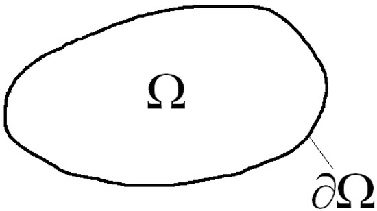
Figure 1.
The bounded open set and its boundary .
Clearly, Problem 1 is one of the most studied and well known mathematical problems. On the other hand, Problem 2 is a nonlinear problem that requires much more effort to be simulated than what is necessary for Problem 1.
In this work, we represent the solution of Problem 2 by means of the solution of problems such as Problem 1, provided the following conditions hold:
- There exists a positive constant such that, for any , ;
- is a non-increasing function of , for any ;
- is a strictly increasing function of , for any ;
- , for any ;
- , for any ;
- , for any ;
- , for any , for any .
In other words, the solution of Problem 2 will be represented by the limit of the sequence , in which
The (known) functions and are obtained from the knowledge of .
It is to be noticed that almost all steady-state heat transfer problems can be described by Problem 2 and satisfy the six above conditions. In addition, it is remarkable that the function always admits an inverse. In fact, when represents the thermal conductivity (or any diffusion coefficient), the existence of a positive lower bound is always ensured.
When Equation (2) represents a heat transfer process, is a heat source (per unit time and per unit volume), is the thermal conductivity, and is the temperature. The function represents the heat loss (per unit time and per unit area) from the body boundary.
The main subject of this work is concerned with real physical applications arising from heat transfer problems. In this way, the domain is assumed to have the cone property and that its boundary is composed by a finite number of smooth parts. In addition, it is assumed that and are bounded and are piecewise continuous functions of for each given . As physically expected, the function (temperature) will be a continuous function in and will satisfy Problem 2 almost everywhere.
It is to be noticed that, in general, real heat transfer problems are nonlinear and usually are simulated under a severe hypothesis in order to avoid complex mathematical tools for their solutions. With the procedure proposed in this work, a large class of nonlinear heat transfer problems can be treated with simple basic tools, such as those used for solving the linear problems. The proposed procedure allows a low-cost simulation for problems that, usually, require sophisticated methods.
In addition, since the solution will be obtained as the limit of a non-decreasing sequence (with a known upper bound), it is easy to verify the consistency of a given simulation. In other words, if the sequence does not behave as expected, the simulation must be stopped, because something must be corrected (probably or is not large enough).
2. Construction of the Non-Decreasing Sequence
Let us consider the problem below:
in which the functions and have the following properties
- is a non-increasing function of , for any ;
- is a strictly increasing function of , for any ;
- , for any ;
- , for any ;
- , for any ;
- , for any , for any .
Thus, the sequence , whose elements are obtained from the solution of
is a convergent non-increasing sequence, provided and are sufficiently large constants in order to ensure that
As a first step, let us prove that is non-negative everywhere. Aiming for this, we write, from Equation (5), for
Now, let us assume that assumes its minimum at a point . Thus, there exists a small neighborhood of in which . Therefore, in this neighborhood, . Since and , we are able to conclude that, if has a local minimum in , then this minimum is non-negative. On the other hand, if this minimum does not occur in , we have that there exists a subset , such that [21,22]
On the subset , from the boundary condition, we have
Therefore, since , we conclude that is non-negative everywhere. Therefore, .
From Equation (5), we may write
Combining Equation (10) with Equation (6), we conclude that, if everywhere, then
and does not reach a minimum in . Again, using Equation (6) and taking into account the boundary conditions, we conclude that
Since , the above result enables us to conclude (non-decreasing sequence) that
3. An Upper Bound for the Sequence
The solution of Equations (4), denoted by , is an upper bound for the elements of the sequence . In order to prove this affirmation, let us combine Equations (4) and (5) to obtain
or, in a more convenient form,
Now, let us suppose that the difference assumes its minimum in . In this case we must have in a small neighborhood of the local minimum. Therefore, in this neighborhood, taking into account Equation (6), we have
On the other hand, if does not assume a minimum in , we must have a subset , such that
and, on this subset, taking into account the boundary conditions and Equation (6),
Thus, it is proven that in . Clearly, it must be proven that (4) admits a solution and that . In the next section, with the aid of a variational formulation, we prove that the solution exists and is unique.
Since (from Equation (5))
we have that
Therefore, (the limit of the sequence consists of a solution of Problem 4, provided it admits a solution).
4. Existence and Uniqueness of the Solution of Equation (4)
The solution of Equation (4) is the field which minimizes the functional , defined by
Since, for any , the following inequality holds:
we ensure that
In addition, since the derivative (with respect to ) of is non-negative and the derivative (with respect to ) of is positive, we may write (convexity of the functional )
A necessary condition for ensuring the equality in Equation (22), for two different functions and , is .
Nevertheless, from the definition of , this constant must be zero for ensuring the equality in (24). Therefore, we conclude that the functional is strictly convex. This ensures the uniqueness of the minimum, provided it exists.
In order to prove the existence of the minimum, it is sufficient to show that the convex functional is such that (coerciveness) [23]
in which is the usual norm of [24].
Taking into account that and considering the behavior of and of , the above limit may be represented as follows:
ensuring the coerciveness (solution existence).
At this point, it is convenient to show that the minimization of corresponds, in a weak sense, to the solution of (4). Aiming to this, based on Equation (21), let us calculate the first variation of as follows
or, in a more convenient way, as
Since [25]
we may write
Thus, taking into account that is arbitrary, gives rise to (Euler–Lagrange equation and natural boundary condition)
proving the equivalence between (4) and the minimization of the functional (note that represents the Laplacian).
In other words, we have that, in a weak sense, (4) admits one, and only one, solution. In fact, this minimum will belong to . Since the domain belongs to and has the cone property, this minimum will be continuous in (Sobolev imbedding theorem [24]).
It is natural to ask about the use of for reaching the solution . Surely, the minimization of is a valid and reliable procedure, but, the procedure proposed in this work is also reliable and involves much more simple tools.
5. Construction of the Solution of Problem 2
Since , the knowledge of the elements of the sequence , as well as its limit, enable us to determine, in a unique way, the elements of the sequence , as well as its limit. In other words, the knowledge of determines, in a unique way, the solution of Problem 2.
The functional relationship between (solution of (4)) and (solution of (2)) depends on the choice of the function . There are infinite possible choices. For instance, when the physically considered range for the temperature is the interval , the function may be defined as [26]
It is to be noticed that, for any real heat transfer process, and are positive valued constants, provided represents an absolute temperature.
In order to illustrate the calculation of from the knowledge of , let us consider a particular case in which, within the physically admissible range,
In this case
and the temperature is given by
The linear relationship between the thermal conductivity and the temperature is the most usual for describing heat transfer processes. Other relationships may be used as, for instance, the one proposed in [26] and used in [27].
Figure 2 illustrates a particular case of Equation (34).
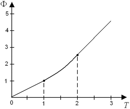
Figure 2.
as a function of for a case in which , , and for .
6. The Constants and
The constants and must satisfy Equation (6). Since (4) admits a unique solution and , the existence of the constants and is ensured.
In order to provide a sufficiently (not necessarily) large value for each of these two constants, it is convenient to establish an upper bound for before solving the problem.
Aiming at this, let us define the function , (any) solution of the following partial differential equation:
For instance, an always possible choice (not a unique choice and, probably, often not the best) for is
Combining Equation (4) with Equation (36), we have
Therefore, there exists a subset in which , such that
Taking into account the boundary condition, we may write
Since,
we are able to write
in which is a known function.
Therefore, any constant satisfying the inequality
will be greater than the supremum of on . Therefore,
Once known, an upper bound for , the constants and may be chosen from the following inequalities (sufficient conditions, but not necessary):
It must be highlighted that and satisfying (45) ensure the convergence of the non-decreasing sequence . Nevertheless, in general, this non-decreasing convergent sequence may be reached with lower values for and .
When and are differentiable with respect to , within the interval of interest, (45) may be rewritten as follows:
Clearly, from Equation (45), if does not depend on , then may be zero.
7. Conclusions
This work provides a powerful and simple tool for simulating any steady-state heat transfer phenomenon and any other process, described by a nonlinear second order partial differential equation such as Equation (2), even when subjected to nonlinear boundary conditions (for instance, arising from thermal radiation heat transfer from/to the body) and involving temperature-dependent source terms (even when this dependence is not linear).
The results presented here generalize common situations in which the source term is assumed to be known (i.e., did not depend on the temperature) and where the boundary condition is the classical linear Newton law of cooling.
The proposed procedure for constructing the solution may be used together with any numerical scheme available for a linear problem such as Problem 1, making a large class of nonlinear problems accessible to any student (of engineering, physics, or mathematics). An example is presented in Appendix A.
The conditions imposed for ensuring the convergence are sufficient conditions, but are not necessary. In other words, the procedure may work even outside of the ensured range.
The disadvantage of the proposed procedure is the fact of not knowing the optimal value of the constant (the lower one which ensures convergence). On the other hand, if the convergence is reached for a given , it will be reached for any greater than .
It is to be noticed that linear problems, in particular those involving linear boundary conditions, admit an equivalent minimum principle represented by a quadratic functional. Nonlinear problems are not equivalent to the minimization of quadratic functionals.
Funding
This research was funded by [CNPq] grant number [306364/2018-1] and by Brazilian Agency CAPES (finance code 001). The APC was funded by CNPq/Brazil.
Conflicts of Interest
The authors declare no conflict of interest.
Appendix A. An Example
In order to explicitly illustrate the solution construction, let us consider the one-dimensional problem below, which represents the heat transfer in a slab with thickness .
In this case, the solution is given by (when we have the linear case)
At the surfaces and , we have the same temperature, given by
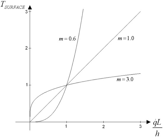
Figure A1.
The temperature at the surface as a function of for three values of .
In order to illustrate the procedure proposed in this work, let us consider the following particular case of Equation (A1):
which describes the coupled conduction–radiation heat transfer process in a black slab (thickness ), represented in a convenient system of units.
The solution is obtained as the limit of the sequence , whose elements are obtained from
in which .
Each element is given by
in which the ’s are constants ().
Figure A2 and Figure A3 below illustrate the convergence process for two different values of the constant . In both cases, the convergence is reached, but the convergence speed for is greater than the convergence speed for .
In fact, as decreases, the convergence speed increases. Nevertheless, very low values of may not give rise to convergence.
For instance, if we consider in Equation (A5), the convergence is not reached. This fact is illustrated in Figure A4, in which is represented as a function of “” for some selected values of the constant .
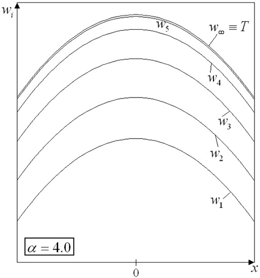
Figure A2.
Some elements of the sequence and its limit (exact solution), obtained with .
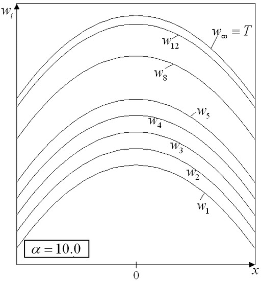
Figure A3.
Some elements of the sequence and its limit (exact solution), obtained with .
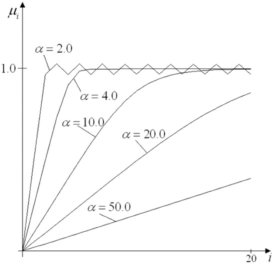
Figure A4.
The constants as a function of the index () for five selected values of .
For sufficiently large , it is to be noticed that, for , represents the temperature at . This is not true for .
In Figure A5, the same result is presented, considering .
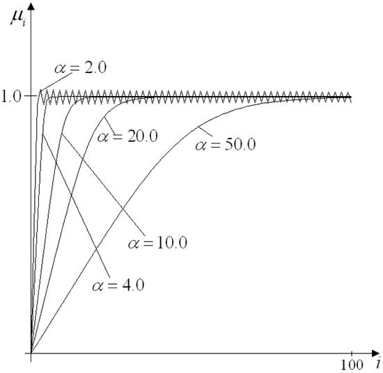
Figure A5.
The constants as a function of the index () for the same previously selected values of .
References
- Holman, J.P. Heat Transfer, 10th ed.; McGraw-Hill: New York, NY, USA, 2009. [Google Scholar]
- Bergman, T.L.; Lavine, A.S.; Incropera, F.P.; Dewitt, D.P. Fundamentals of Heat and Mass Transfer, 7th ed.; John Wiley & Sons, Inc.: Danvers, MA, USA, 2007. [Google Scholar]
- Kreith, F.; Manglik, R.M. Principles of Heat Transfer, 8th ed.; CENGAGE Learning: Boston, MA, USA, 2011. [Google Scholar]
- Slattery, J.C. Momentum, Energy and Mass Transfer in Continua; McGraw-Hill Kogakusha: Tokyo, Japan, 1972. [Google Scholar]
- Carslaw, H.S.; Jaeger, J.C. Conduction of Heat in Solids, 2nd ed.; Oxford University Press: New York, NY, USA, 2000. [Google Scholar]
- Arpaci, V.S. Conduction Heat Transfer; Addison-Wesley Publishing Company: Boston, MA, USA, 1966. [Google Scholar]
- Goldberg, Y.; Levinshtein, M.E.; Rumyantsev, S.L. Properties of Advanced Semiconductor Materials GaN, AlN, SiC, BN, SiC, SiGe; Levinshtein, M.E., Rumyantsev, S.L., Shur, M.S., Eds.; John Wiley & Sons, Inc.: New York, NY, USA, 2001; pp. 93–148. [Google Scholar]
- Woodcraft, A. Recommended values for the thermal conductivity of aluminium of different purities in the cryogenic to room temperature range, and a comparison with copper. Cryogenics 2005, 45, 626–636. [Google Scholar] [CrossRef]
- Joyce, W. Thermal resistance of heat sinks with temperature-dependent conductivity. Solid-State Electron. 1975, 18, 321–322. [Google Scholar] [CrossRef]
- Gama, R.M.S. Closed-form formulae for the Kirchhoff transformation assuming a piecewise constant temperature dependent thermal conductivity. Lat. Am. Appl. Res. 2017, 47, 53–57. [Google Scholar] [CrossRef]
- Afrin, N.; Feng, Z.C.; Zhang, Y.; Chen, J.K. Inverse estimation of front surface temperature of a locally heated plate with temperature-dependent conductivity via Kirchhoff transformation. Int. J. Therm. Sci. 2013, 69, 53–60. [Google Scholar] [CrossRef]
- Chantasiriwan, S. Steady-state determination of temperature-dependent thermal conductivity. Int. Commun. Heat Mass Transf. 2002, 29, 811–819. [Google Scholar] [CrossRef]
- Mierzwiczak, M.; Kołodziej, J. The determination temperature-dependent thermal conductivity as inverse steady heat conduction problem. Int. J. Heat Mass Transf. 2011, 54, 790–796. [Google Scholar] [CrossRef]
- Kim, S. A simple direct estimation of temperature-dependent thermal conductivity with Kirchhoff transformation. Int. Commun. Heat Mass Transf. 2001, 28, 537–544. [Google Scholar] [CrossRef]
- Moitsheki, R.J.; Hayat, T.; Malik, M.Y. Some exact solutions for a fin problem with a power law temperature-dependent thermal conductivity. Nonlinear Anal. Real World Appl. 2010, 11, 3287–3294. [Google Scholar] [CrossRef]
- Yeih, W.; Chan, I.Y.; Fan, C.M.; Chang, J.J.; Liu, C. Solving the Cauchy problem of the nonlinear steady-state heat equation using double iteration process. CMES-Comp. Model. Eng. 2014, 99, 169–194. [Google Scholar]
- Nedjar, B. An enthalpy-based finite element method for nonlinear heat problems involving phase change. Comp. Struct. 2002, 80, 9–21. [Google Scholar] [CrossRef]
- Jordan, P.M. A Nonstandard finite difference scheme for nonlinear heat transfer in a thin finite rod. J. Differ. Equations Appl. 2003, 9, 1015–1021. [Google Scholar] [CrossRef]
- Ahmad, I.; Khaliq, A.Q. Local RBF method for multi-dimensional partial differential equations. Comp. Math. Appl. 2017, 74, 292–324. [Google Scholar] [CrossRef]
- Yeih, W. Solving the nonlinear heat equilibrium problems using the local multiquadric radial basis function collocation method. Mathematics 2020, 8, 1289. [Google Scholar] [CrossRef]
- John, F. Partial Differential Equations; Springer: New York, NY, USA, 1981. [Google Scholar]
- Courant, R.; John, F. Introduction to Calculus and Analysis; Springer: New York, NY, USA, 1989; Volume 2. [Google Scholar]
- Berger, M.S. Nonlinearity & Functional Analysis: Lectures on Nonlinear Problems in Mathematical Analysis; Academic Press: London, UK, 1977. [Google Scholar]
- Adams, R.A. Sobolev Spaces; Academic Press: New York, NY, USA, 1975. [Google Scholar]
- Wylie, C.R. Advanced Engineering Mathematics; McGraw-Hill Kogakusha: Tokyo, Japan, 1975. [Google Scholar]
- Martins-Costa, M.L.; Freitas Rachid, F.B.; Gama, R.M.S. An unconstrained mathematical description for conduction heat transfer problems with linear temperature-dependent thermal conductivity. Int. J. Non-Linear Mech. 2016, 81, 310–315. [Google Scholar]
- Gama, R.M.S.; Corrêa, E.D.; Martins-Costa, M.L. An upper bound estimate for the steady-state temperature for a class of heat conduction problems wherein the thermal conductivity is temperature dependent. Int. J. Eng. Sci. 2013, 69, 77–83. [Google Scholar] [CrossRef]
Publisher’s Note: MDPI stays neutral with regard to jurisdictional claims in published maps and institutional affiliations. |
© 2022 by the author. Licensee MDPI, Basel, Switzerland. This article is an open access article distributed under the terms and conditions of the Creative Commons Attribution (CC BY) license (https://creativecommons.org/licenses/by/4.0/).