The Darboux Transformation and N-Soliton Solutions of Gerdjikov–Ivanov Equation on a Time–Space Scale

Abstract

The Gerdjikov–Ivanov (GI) equation is one type of derivative nonlinear Schrödinger equation used widely in quantum field theory, nonlinear optics, weakly nonlinear dispersion water waves and other fields. In this paper, the coupled GI equation on a time–space scale is deduced from Lax pairs and the zero curvature equation on a time–space scale, which can be reduced to the classical and the semi-discrete GI equation by considering different time–space scales. Furthermore, the Darboux transformation (DT) of the GI equation on a time–space scale is constructed via a gauge transformation. Finally, N-soliton solutions of the GI equation are given through applying its DT, which are expressed by the Cayley exponential function. At the same time, one-solition solutions are obtained on three different time–space scales ( $\mathbb{X}$ = $\mathbb{R}$, $\mathbb{X}$ = $\mathbb{C}$ and $\mathbb{X}$ = $\mathbb{K}p$ ).

1. Introduction

There are some practical problems that cannot be solved accurately by using only continuous or discrete analysis. In order to unify continuous and discrete analysis, a time scale was initiated by Stefan Hilger in 1988, which is an arbitrary nonempty closed subset of the real numbers [1,2,3]. In recent years, extensive research about time scales has been conducted, particularly in stability, oscillation and initial-boundary value problems [4,5,6,7,8]. In addition, time scale dynamic equations have wide application prospects in many areas, such as population dynamic models [9], epidemic models [10,11] and models of the financial consumption process [12,13].

Toda’s lattice, Hirota’s network and nonlinear Schrödinger dynamic equations were derived on a time–space scale by extending an Ablowitz–Ladik hierarchy of integrable dynamic systems on a time–space scale [14]. This extension facilitates a variety of modeling applications of Ablowitz–Ladik hierarchies, including optics and chaos in dispersion numerical schemes [15]. The formulas for solutions of boundary value problem of Burgers equation and heat equation were derived on a time–space scale by using the Cole–Hopf transformation. These formulas may be used to study the wave motion on a time–space scale. Sine-Gordon equation was obtained on a time–space scale and its solution expressed by the Cayley exponential function was given [16,17,18]. However, the development of time–space scales is relatively slow in nonlinear dynamical systems compared to other fields.

There are important applications regarding the derivative nonlinear Schrödinger (DNLS) equation in many fields [19]. In particular, in situations where higher order nonlinear effects need to be restored, a family of DNLS equations was investigated [20]. There are three famous DNLS equations, which are the DNLS I equation [21,22], DNLS II equation [23,24] and DNLS III equation [25]. The forms of these three equations are as follows

$$i{q}_t+q_{xx}+i{\left(q^2{q}^{*}\right)}_x=0,$$

$$i{q}_t+q_{xx}+iq{q}^{*}{q}_x=0,$$

$$i{q}_t+q_{xx}+\frac{1}{2}{q}^3{q}^{*2}-i{q}^2{q}_x^{*}=0,$$

where $q*$ represents the complex conjugate of q. They can be transformed into each other by a gauge transformation [26]. Specifically, the last equation is also known as the Gerdjikov–Ivanov (GI) equation, which was discovered by Gerdjikov and Ivanov [27]. In recent years, several useful methods have been proposed for obtaining solutions of the GI equation, such as the Darboux transformation (DT) [28,29], algebra-geometric solution [30,31,32,33], Wronskian type solution [29,34] and Hamiltonian structures [35,36].

The advantage of DT is that new solutions can be obtained successively through iteration. The explicit soliton-like solution of the GI equation was obtained by its DT [26]. The explicit N-fold DT with multiparameters for the GI equation was constructed with the help of a gauge transformation [28]. The dark soliton, bright soliton, breather solution and periodic solution are given explicitly from different seed solutions. In this paper, the coupled GI equation on a time–space scale is deduced by the Lax matrix equation extended on a time–space scale. This extension will provide a wider range of nonlinear integrable dynamic models and promote solutions to practical problems.

This paper is organized as follows. In Section 2, the coupled GI equation on a time–space scale is obtained, which can be reduced to the classical and the semi-discrete GI equation. In Section 3, N-fold DT and N-soliton solutions of the GI equation on a time–space scale are constructed with the help of a gauge transformation. In particular, one-soliton solutions of the GI equation on three different time–space scales are obtained from seed solution. The last section is our conclusions.

2. GI Equation on a Time–Space Scale

For constructing the GI equation on a time–space scale, jump operators, graininess functions and the $\nabla -$ derivative are introduced as follows [1,2,3].

Definition 1.

For $\left(t,x\right)\in \mathbb{T}\times \mathbb{X}$, backward jump operators are defined as

$$\sigma :\mathbb{T}\to \mathbb{T},\rho :\mathbb{X}\to \mathbb{X},$$

$$\sigma \left(t\right)=sup\left\{s\in \mathbb{T}:s<t\right\},\rho \left(x\right)=sup\left\{y\in \mathbb{X}:y<x\right\}.$$

(1)

For $x\in \mathbb{X}$, the forward jump operator $\beta \left(x\right):\mathbb{X}\to \mathbb{X}$ is defined as $\beta \left(x\right)={\rho }^{-1}\left(x\right)=inf\left\{y\in \mathbb{X}:y>x\right\}$.

Definition 2.

The $\nabla -$ derivative associated with t (time) and x (space) variables is defined as

$${\nabla }_{t}f\left(t,x\right)=\underset{p\to \mu \left(t\right)}{lim}\frac{f\left(t,x\right)-f^{\sigma }\left(t,x\right)}{p},$$

(2)

$${\nabla }_{x}f\left(t,x\right)=\underset{q\to \nu \left(x\right)}{lim}\frac{f\left(t,x\right)-f^{\rho }\left(t,x\right)}{q},$$

(3)

where the graininess functions $\mu :\mathbb{T}\to [0,+\infty ),\nu :\mathbb{X}\to [0,+\infty )$ are defined as

$$\mu \left(t\right)=t-\sigma \left(t\right),\nu \left(x\right)=x-\rho \left(x\right).$$

(4)

Note that,

$$f^{\sigma }(t,x):=f(\sigma \left(t\right),x)=f\left(t,x\right)-\mu \left(t\right){\nabla }_{t}f\left(t,x\right),$$

(5)

$$f^{\rho }(t,x):=f(t,\rho \left(x\right))=f\left(t,x\right)-\nu \left(x\right){\nabla }_{x}f\left(t,x\right).$$

(6)

Definition 3.

The Cayley exponential function on a time scale is defined by

$$e_{\alpha }\left(x,x_0\right):=exp\left({\int }_{{\iota }_0}^x{\zeta }_{\mu \left(s\right)}\left(\alpha \left(s\right)\right)\mathsf{\Delta }s\right),e_{\alpha }\left(x\right):=e_{\alpha }(x,0),$$

where $\alpha =\alpha \left(x\right)$ is a given rd-continuous regressive function and

$${\zeta }_h\left(z\right):=\frac{1}{h}log\frac{1+\frac{1}{2}zh}{1-\frac{1}{2}zh},h>0,{\zeta }_0\left(z\right):=z.$$

When $\mathbb{X}=\mathbb{R}$ and $\mathbb{X}=h\mathbb{Z}$, the Cayley exponential function becomes

$$\begin{array}{cc}& e_{\alpha }\left(x\right)=e^{{\int }_0^x\alpha \left(s\right)ds}and\hfill \\ & e_{\alpha }\left(x\right)={\left(\frac{1+\frac{1}{2}\alpha h}{1-\frac{1}{2}\alpha h}\right)}^{\frac{x}{h}},\hfill \end{array}$$

respectively.

Lemma 1.

Take $\mathbb{T}\times \mathbb{X}=\mathbb{R}\times \mathbb{R}$. The backward jump operators

$$\sigma \left(t\right)=sup\left(-\infty ,t\right)=t,\rho \left(x\right)=sup\left(-\infty ,x\right)=x,$$

(7)

and the graininess functions

$$\mu \left(t\right)=t-\sigma \left(t\right)=0,\nu \left(x\right)=x-\rho \left(x\right)=0.$$

(8)

Lemma 2.

Take $\mathbb{T}\times \mathbb{X}=\mathbb{R}\times \mathbb{Z}$. The backward jump operators

$$\sigma \left(t\right)=sup\left(-\infty ,t\right)=t,\rho \left(x\right)=sup\{x-1,x-2,\cdots \}=x-1,$$

(9)

and the graininess functions

$$\mu \left(t\right)=t-\sigma \left(t\right)=0,\nu \left(x\right)=x-\rho \left(x\right)=1.$$

(10)

Lemma 3.

When $\mathbb{X}=\mathbb{R}$, $\mathbb{X}=\hslash \mathbb{Z}$ and $\mathbb{X}={\mathbb{K}}_p$, the $\nabla -$ derivative becomes

$$\begin{array}{cc}& {\nabla }_{x}f\left(x\right)=f_x\left(x\right),\hfill \\ & {\nabla }_{x}f\left(x\right)=\frac{f\left(x\right)-f(x-\hslash )}{\hslash }and\hfill \\ & {\nabla }_{x}f\left(x\right)=\frac{f\left(x\right)-f\left(p^{-1}x\right)}{\left(1-p^{-1}\right)x},\hfill \end{array}$$

respectively.

In what follows, based on Lax pairs of DNLS equation from the generalized Kaup–Newell spectrum problem [32], a ∇-dynamical system is introduced

$$\left\{\begin{array}{c}\hfill {\nabla }_x\psi \left(t,x\right)=U\left(t,x\right)\psi \left(t,x\right),\\ \hfill {\nabla }_t\psi \left(t,x\right)=V\left(t,x\right)\psi \left(t,x\right),\end{array}\right.$$

(11)

where

$$\left\{\begin{array}{cc}\hfill U& =\left(\begin{array}{cc}-i{\lambda }^2-\frac{1}{2}iqr& \lambda q\\ \lambda r& i{\lambda }^2+\frac{1}{2}iqr\end{array}\right),\hfill \\ \hfill V& =\left(\begin{array}{cc}A\left(t,x\right)& B\left(t,x\right)\\ C\left(t,x\right)& -A\left(t,x\right)\end{array}\right),\hfill \end{array}\right.$$

(12)

with $\psi =\left(\begin{array}{c}{\psi }_1\left(t,x\right)\\ {\psi }_2\left(t,x\right)\end{array}\right)$, q and r are potential functions, and $\lambda$ is a spectral parameter.

According to the compatibility condition ${\nabla }_{xt}\psi ={\nabla }_{tx}\psi$ and $\nabla -$ derivative product rules [15], the zero curvature equation on a time–space scale is obtained

$${\nabla }_{t}U-{\nabla }_{x}V+U^{\sigma }V-V^{\rho }U=0.$$

(13)

Then, substituting Equation (12) into Equation (13), we find

$$\begin{array}{c}\hfill \left\{\begin{array}{c}-i\left(C+C^{\rho }\right){\lambda }^2-\left(r^{\sigma }A+r{A}^{\rho }+{\nabla }_{t}r\right)\lambda -\frac{1}{2}i{\left(qr\right)}^{\sigma }C-\frac{1}{2}iqr{C}^{\rho }+{\nabla }_{x}C=0,\hfill \\ -i\left(B+B^{\rho }\right){\lambda }^2-\left(q^{\sigma }A+q{A}^{\rho }+{\nabla }_{t}q\right)\lambda -\frac{1}{2}i{\left(qr\right)}^{\sigma }B-\frac{1}{2}iqr{B}^{\rho }-{\nabla }_{x}B=0,\hfill \\ -i\left(A-A^{\rho }\right){\lambda }^2+\left(q^{\sigma }C-r{B}^{\rho }\right)\lambda -\frac{1}{2}i{\left(qr\right)}^{\sigma }A+\frac{1}{2}iqr{A}^{\rho }-\frac{1}{2}i{\nabla }_t\left(qr\right)-{\nabla }_{x}A=0,\hfill \\ -i\left(A-A^{\rho }\right){\lambda }^2+\lambda \left(r^{\sigma }B-q{C}^{\rho }\right)-\frac{1}{2}i{\left(qr\right)}^{\sigma }A+\frac{1}{2}iqr{A}^{\rho }-\frac{1}{2}i{\nabla }_t\left(qr\right)+{\nabla }_{x}A=0.\hfill \end{array}\right.\end{array}$$

(14)

Take A, B and C as quaternary polynomials of $\lambda$,

$$A=\sum _{j=0}^4{a}_j{\lambda }^j,B=\sum _{j=0}^4{b}_j{\lambda }^j,C=\sum _{j=0}^4{c}_j{\lambda }^j.$$

(15)

Then, by substituting Equation (15) into Equation (14), these relations are obtained

$$\begin{array}{c}\hfill \left\{\begin{array}{cc}\hfill a_4=& -2i,a_1=a_3=b_0=b_2=b_4=c_0=c_2=c_4=0,\hfill \\ \hfill b_3=& -b_3^{\rho }+2\left(q^{\sigma }+q\right),c_3=-c_3^{\rho }+2\left(r^{\sigma }+r\right)=0,\hfill \\ \hfill b_1=& -b_1^{\rho }+iq{a}_2^{\rho }+i{q}^{\sigma }{a}_2-\frac{1}{2}qr{b}_3^{\rho }-\frac{1}{2}{\left(qr\right)}^{\sigma }{b}_3+i{\nabla }_x{b}_3,\hfill \\ \hfill c_1=& -c_1^{\rho }+ir{a}_2^{\rho }+i{r}^{\sigma }{a}_2-\frac{1}{2}qr{c}_3^{\rho }-\frac{1}{2}{\left(qr\right)}^{\sigma }{c}_3-i{\nabla }_x{c}_3,\hfill \\ \hfill a_2=& {\nabla }_x^{-1}(\frac{1}{2}{q}^{\sigma }{c}_1-\frac{1}{2}{r}^{\sigma }{b}_1-\frac{1}{2}r{b}_1^{\rho }+\frac{1}{2}q{c}_1^{\rho }),\hfill \\ \hfill a_0=& {\nabla }_x^{-1}(-\frac{1}{2}iq{r}^{\sigma }{a}_0^{\rho }+\frac{1}{4}qr{r}^{\sigma }{b}_1^{\rho }-\frac{1}{2}i{r}^{\sigma }{b}_1^x-\frac{1}{2}i{q}^{\sigma }{r}^{\sigma }{a}_0+\frac{1}{4}{\left(qr\right)}^{\sigma }{b}_1{r}^{\sigma }\hfill \\ \hfill & +\frac{1}{2}iqr{a}_0^{\rho }-\frac{1}{4}{q}^{2}r{c}_1^{\rho }+\frac{1}{2}i{r}^{\sigma }q{a}_0-\frac{1}{4}{\left(qr\right)}^{\sigma }q{c}_1-\frac{1}{2}i{c_1}_{x}q),\hfill \end{array}\right.\end{array}$$

(16)

and evolution equations on a time–space scale are obtained

$${\nabla }_{t}q=q{a}_0^{\rho }+q^{\sigma }{a}_0+\frac{1}{2}iqr{b}_1^{\rho }+\frac{1}{2}i{\left(qr\right)}^{\sigma }{b}_1+{\nabla }_x{b}_1,$$

(17)

$${\nabla }_{t}r=-r{a}_0^{\rho }-r^{\sigma }{a}_0-\frac{1}{2}iqr{c}_1^{\rho }-\frac{1}{2}i{\left(qr\right)}^{\sigma }{c}_1+{\nabla }_x{c}_1.$$

(18)

According to Equations (5) and (6), Equation (16) is reduced to

$$b_3=2{\left(2-\nu \left(x\right){\nabla }_x\right)}^{-1}\left(q+q^{\sigma }\right),$$

(19)

$$c_3=2{\left(2-\nu \left(x\right){\nabla }_x\right)}^{-1}\left(r+r^{\sigma }\right),$$

(20)

$$b_1=2i{\left(2-\nu \left(x\right){\nabla }_x\right)}^{-1}{m}_1{a}_2+\frac{1}{2}{\left(2-\nu \left(x\right){\nabla }_x\right)}^{-1}{m}_4\left(q+q^{\sigma }\right),$$

(21)

$$c_1=2i{\left(2-\nu \left(x\right){\nabla }_x\right)}^{-1}{m}_2{a}_2+\frac{1}{2}{\left(2-\nu \left(x\right){\nabla }_x\right)}^{-1}{m}_3\left(r+r^{\sigma }\right),$$

(22)

$${\nabla }_x{a}_0=\frac{1}{2}i{m}_5{a}_0+\frac{1}{2}i\left(r^{\sigma }{m}_4{m}_1-q{m}_4{m}_2\right)a_2+\frac{1}{8}{r}^{\sigma }{m}_4^2\left(q+q^{\sigma }\right)-\frac{1}{8}q{m}_4{m}_3\left(r+r^{\sigma }\right),$$

(23)

$${\nabla }_x{a}_2=\frac{1}{2}i\left(m_1{m}_2-m_2{m}_1\right)\left(2-\nu \left(x\right){\nabla }_x\right)a_2+\frac{1}{2}{m}_1{m}_3\left(r+r^{\sigma }\right)+\frac{1}{2}{m}_2{m}_4\left(q+q^{\sigma }\right),$$

(24)

with

$$\begin{array}{cc}\hfill & m_1=\left[q^{\sigma }+q\left(1-\nu \left(x\right){\nabla }_x\right)\right]{\left(2-\nu \left(x\right){\nabla }_x\right)}^{-1},\hfill \\ \hfill & m_2=\left[r^{\sigma }+r\left(1-\nu \left(x\right){\nabla }_x\right)\right]{\left(2-\nu \left(x\right){\nabla }_x\right)}^{-1},\hfill \\ \hfill & m_3=\left[{\left(qr\right)}^{\sigma }+\left(qr\right)\left(1-\nu \left(x\right){\nabla }_x\right)+2i{\nabla }_x\right]{\left(2-\nu \left(x\right){\nabla }_x\right)}^{-1},\hfill \\ \hfill & m_4=\left[{\left(qr\right)}^{\sigma }+\left(qr\right)\left(1-\nu \left(x\right){\nabla }_x\right)-2i{\nabla }_x\right]{\left(2-\nu \left(x\right){\nabla }_x\right)}^{-1},\hfill \\ \hfill & m_5=\left(qr-q{r}^{\sigma }\right)\left(1-\nu \left(x\right){\nabla }_x\right)+q{r}^{\sigma }-q^{\sigma }{r}^{\sigma }.\hfill \end{array}$$

Then, the coupled GI equation on a time–space scale is obtained

$$\begin{array}{c}\hfill \left\{\begin{array}{cc}\hfill {\nabla }_{t}q=& q\left(1-\nu \left(x\right){\nabla }_x\right)a_0+q^{\sigma }{a}_0+\frac{1}{2}iqr\left(1-\nu \left(x\right){\nabla }_x\right)b_1+\frac{1}{2}i{\left(qr\right)}^{\sigma }{b}_1+{\nabla }_x{b}_1,\hfill \\ \hfill {\nabla }_{t}r=& -r\left(1-\nu \left(x\right){\nabla }_x\right)a_0-r^{\sigma }{a}_0-\frac{1}{2}iqr\left(1-\nu \left(x\right){\nabla }_x\right)c_1-\frac{1}{2}i{\left(qr\right)}^{\sigma }{c}_1+{\nabla }_x{c}_1,\hfill \end{array}\right.\end{array}$$

(25)

where $a_0,b_1,c_1$ are defined by Equations (21)–(23), respectively.

In the following, two special kinds of equations are given as follows.

Case I: Taking $\mathbb{T}\times \mathbb{X}=\mathbb{R}\times \mathbb{R}$, we find $\mu \left(t\right)=0,\nu \left(x\right)=0$.

Equations (21)–(23) are reduced to

$$\begin{array}{cc}& b_1=i{q}_x,\hfill \\ & c_1=-i{r}_x,\hfill \\ & a_0=\frac{1}{2}\left(r{q}_x-q{r}_x\right)+\frac{1}{4}i{q}^2{r}^2.\hfill \end{array}$$

Then, Equation (25) is reduced to the coupled GI equation

$$\begin{array}{c}\hfill \left\{\begin{array}{c}\hfill i{q}_t+q_{xx}+i{q}^2{r}_x+\frac{1}{2}{q}^3{r}^2=0,\\ \hfill i{r}_t-r_{xx}+i{r}^2{q}_x-\frac{1}{2}{q}^2{r}^3=0.\end{array}\right.\end{array}$$

(26)

When $r=-q^{*}$, the classical GI equation is obtained

$$i{q}_t+q_{xx}+\frac{1}{2}{q}^3{q^{*}}^2-i{q}^2{q}_x^{*}=0.$$

(27)

Case II: Taking $\mathbb{T}\times \mathbb{X}=\mathbb{R}\times \mathbb{Z}$, we find $\mu \left(t\right)=0,\nu \left(x\right)=1$.

$$\begin{array}{cc}\hfill & f^{\sigma }(x,t)=f(x,t),\hfill \\ \hfill & f^{\rho }(x,t)=Ef(x,t)=f(x,t)-(1-E)f(x,t),\hfill \end{array}$$

(28)

where E is the shift operator. Then, Equations (19)–(24) are reduced to

$$b_3=4{(1+E)}^{-1}q,$$

(29)

$$c_3=4{(1+E)}^{-1}r,$$

(30)

$$a_2={(1-E)}^{-1}\left(q{r}^2+r{m}_{7}q\right),$$

(31)

$$b_1=2i{(1+E)}^{-1}q{(1-E)}^{-1}\left(q{r}^2+r{m}_{7}q\right)+{(1+E)}^{-1}{m}_{7}q,$$

(32)

$$c_1=2i{(1+E)}^{-1}r{(1-E)}^{-1}\left(q{r}^2+r{m}_{7}q\right)+{(1+E)}^{-1}{m}_{6}q,$$

(33)

$$\begin{array}{cc}\hfill a_0=& \frac{1}{2}i{(1-E)}^{-1}\left(r{m}_{7}q-q{m}_{7}r\right){(1-E)}^{-1}\left(q{r}^2+r{m}_{7}q\right)\hfill \\ \hfill & +\frac{1}{4}{(1-E)}^{-1}\left(r{m}_7^{2}q-q{m}_7{m}_{6}r\right),\hfill \end{array}$$

(34)

with

$$\begin{array}{cc}\hfill & m_6=qr+2i(1-E){(1+E)}^{-1},\hfill \\ \hfill & m_7=qr-2i(1-E){(1+E)}^{-1}.\hfill \end{array}$$

Therefore, the semi-discrete coupled GI equation is obtained

$$\begin{array}{cc}\hfill & q_t=q(1+E)a_0+\frac{1}{2}iqr(1+E)b_1+(1-E)b_1,\hfill \\ \hfill & r_t=-r(1+E)a_0-\frac{1}{2}iqr(1+E)c_1+(1-E)c_1,\hfill \end{array}$$

(35)

where $a_0,b_1,$ and $c_1$ are defined by Equations (32)–(34), respectively.

3. DT of GI Equation on a Time–Space Scale

In this section, we construct a DT for GI equation and give its N-soliton solutions on a time–space scale.

3.1. Construction of DT on a Time–Space Scale

First, it can be shown by long calculations that Equation (12) is transformed to

$$\begin{array}{c}\hfill \left\{\begin{array}{cc}\hfill U& =-i{\lambda }^2{\sigma }_3+\lambda Q-\frac{1}{2}i{Q}^2{\sigma }_3,\hfill \\ \hfill V& =-2i{\sigma }_3{\lambda }^4+B_3{\lambda }^3+a_2{\sigma }_3{\lambda }^2+B_1\lambda +a_0{\sigma }_3,\hfill \end{array}\right.\end{array}$$

(36)

with ${\sigma }_3$ is a Pauli matrix where $Q=\left(\begin{array}{cc}0& q\\ -q^{*}& 0\end{array}\right)$, $B_1=\left(\begin{array}{cc}0& b_1\\ c_1& 0\end{array}\right)$, $B_3=\left(\begin{array}{cc}0& b_3\\ c_3& 0\end{array}\right)$, $a_j(j=0,2),b_j,c_j(j=1,3)$ are defined by Equations (19)–(24), respectively.

Then, the ∇-dynamical system Equation (11) is transformed into

$$\left\{\begin{array}{c}\hfill {\nabla }_x\psi \left[1\right]=U\left[1\right]\psi \left[1\right],\\ \hfill {\nabla }_t\psi \left[1\right]=V\left[1\right]\psi \left[1\right],\end{array}\right.$$

(37)

under a gauge transformation

$$\psi \left[1\right]=T\left[1\right]\psi .$$

(38)

Substituting Equation (38) into Equation (37), we find

$$U\left[1\right]T\left[1\right]={\nabla }_{x}T\left[1\right]+T{\left[1\right]}^{\rho }U,$$

(39)

$$V\left[1\right]T\left[1\right]={\nabla }_{t}T\left[1\right]+T{\left[1\right]}^{\sigma }V,$$

(40)

where

$$\left\{\begin{array}{cc}\hfill U\left[1\right]& =-i{\lambda }^2{\sigma }_3+\lambda Q\left[1\right]-\frac{1}{2}iQ{\left[1\right]}^2{\sigma }_3,\hfill \\ \hfill V\left[1\right]& =-2i{\sigma }_3{\lambda }^4+B_3\left[1\right]{\lambda }^3+a_2\left[1\right]{\sigma }_3{\lambda }^2+B_1\left[1\right]\lambda +a_0\left[1\right]{\sigma }_3,\hfill \end{array}\right.$$

(41)

with $Q\left[1\right]=\left(\begin{array}{cc}0& q\left[1\right]\\ -q{\left[1\right]}^{*}& 0\end{array}\right)$, $B_1\left[1\right]=\left(\begin{array}{cc}0& b_1\left[1\right]\\ c_1\left[1\right]& 0\end{array}\right)$, $B_3\left[1\right]=\left(\begin{array}{cc}0& b_3\left[1\right]\\ c_3\left[1\right]& 0\end{array}\right)$.

Assume

$$T\left[1\right]=T_0+T_1\lambda$$

(42)

where $T_0=\left(\begin{array}{cc}a& b\\ c& d\end{array}\right),T_1=\left(\begin{array}{cc}{a}_{11}& b_{12}\\ c_{21}& d_{22}\end{array}\right)$.

Substituting Equation (42) into Equation (39) and comparing the coefficients in the terms of the same powers ${\lambda }^j(j=0,\cdots ,5)$ on both sides of equation, we find

$$\left\{\begin{array}{c}{c}_{21}=b_{12}=0,\hfill \\ a_{11}=d_{22}=1,\hfill \\ q\left[1\right]=q+ib+i{b}^{\rho },\hfill \\ q{\left[1\right]}^{*}=q^{*}+ic+i{c}^{\rho }.\hfill \end{array}\right.$$

(43)

Setting $S=-T_0=\left(\begin{array}{cc}{s}_{11}& s_{12}\\ s_{21}& s_{22}\end{array}\right)$, we obtain

$$T\left[1\right]=\lambda I-S,$$

(44)

$$q\left[1\right]=q-i{s}_{12}-i{s}_{12}^{\rho }.$$

(45)

Substituting Equation (44) into Equation (39), we obtain

$${\nabla }_{x}S=\frac{1}{2}i{S}^{\rho }{Q}^2{\sigma }_3+\frac{1}{2}iS{Q}^2{\sigma }_3+Q{S}^2-S^{\rho }QS+i{S}^{\rho }{S}^2{\sigma }_3+i{S}^3{\sigma }_3.$$

(46)

Assume

$$S=H\mathrm{\Lambda }{H}^{-1}$$

(47)

with $\Lambda =\left(\begin{array}{cc}\lambda & 0\\ 0& {\lambda }^{*}\end{array}\right)$ is an eigenvalue matrix, $H=\left(\begin{array}{cc}{\psi }_1& {\psi }_2^{*}\\ {\psi }_2& -{\psi }_1^{*}\end{array}\right)$ is a fundamental solution matrix and satisfies

$$\left\{\begin{array}{cc}\hfill {\nabla }_{x}H& =-i{\sigma }_{3}H{\Lambda }^2+QH\Lambda -\frac{1}{2}i{Q}^2{\sigma }_{3}H,\hfill \\ \hfill {\nabla }_{t}H& =-2i{\sigma }_{3}H{\Lambda }^4+B_3{\Lambda }^3+a_2{\sigma }_{3}H{\Lambda }^2+B_{1}H\Lambda +a_0{\sigma }_{3}H.\hfill \end{array}\right.$$

(48)

It is easy to obtain

$$\begin{array}{cc}\hfill {\nabla }_{x}S& ={\nabla }_x\left(H\Lambda H^{-1}\right)\hfill \\ \hfill & =\frac{1}{2}i{S}^{\rho }{Q}^2{\sigma }_3+\frac{1}{2}iS{Q}^2{\sigma }_3+Q{S}^2-S^{\rho }QS+i{S}^{\rho }{S}^2{\sigma }_3+i{S}^3{\sigma }_3,\hfill \end{array}$$

(49)

which means that Equation (47) yields Equation (46). From $T{\left[1\right]}_t+T{\left[1\right]}^{\sigma }V=V\left[1\right]T\left[1\right]$, we find

$$\begin{array}{cc}\hfill & -{\nabla }_{t}S+\left(\lambda I-S^{\sigma }\right)\left(-2i{\sigma }_3{\lambda }^4+B_3{\lambda }^3+a_2{\sigma }_3{\lambda }^2+B_1\lambda +a_0{\sigma }_3\right)\hfill \\ \hfill =& \left(-2i{\sigma }_3{\lambda }^4+B_3\left[1\right]{\lambda }^3+a_2\left[1\right]{\sigma }_3{\lambda }^2+B_1\left[1\right]\lambda +a_0\left[1\right]{\sigma }_3\right)\left(\lambda I-S\right).\hfill \end{array}$$

(50)

Comparing the coefficients in terms of the same powers ${\lambda }^j(j=0,\cdots ,5)$ on both sides of Equation (50), we obtain

$$\begin{array}{cc}\hfill & {\lambda }^0:-{\nabla }_{t}S-a_0{S}^{\sigma }{\sigma }_3=-a_0\left[1\right]{\sigma }_{3}S,\hfill \\ \hfill & {\lambda }^1:a_0{\sigma }_3-S^{\sigma }{B}_1=-B_1\left[1\right]S+a_0\left[1\right]{\sigma }_3,\hfill \\ \hfill & {\lambda }^2:B_1-a_2{S}^{\sigma }{\sigma }_3=B_1\left[1\right]-a_2\left[1\right]{\sigma }_{3}S,\hfill \\ \hfill & {\lambda }^3:a_2{\sigma }_3-S^{\sigma }{B}_3=a_2\left[1\right]{\sigma }_3-B_3\left[1\right]S,\hfill \\ \hfill & {\lambda }^4:B_3+2i{S}^{\sigma }{\sigma }_3=B_3\left[1\right]+2i{\sigma }_{3}S,\hfill \\ \hfill & {\lambda }^5:-2i{\sigma }_3=-2i{\sigma }_3.\hfill \end{array}$$

(51)

Then, the gauge transformations Equations (44) and (45) are proven to be DT of the GI equation on a time–space scale.

3.2. Soliton Solutions of the GI Equation on a Time–Space Scale

Soliton solutions of the GI equation on a time–space scale are constructed by applying its DT. First, Equation (11) is transformed to

$$\left\{\begin{array}{cc}\hfill {\nabla }_x\psi \left[0\right]& =U\left[0\right]\psi \left[0\right]=\left(\begin{array}{cc}-i{\lambda }^2+\frac{1}{2}iq\left[0\right]q{\left[0\right]}^{*}& \lambda q\left[0\right]\\ -\lambda q{\left[0\right]}^{*}& i{\lambda }^2-\frac{1}{2}iq\left[0\right]q{\left[0\right]}^{*}\end{array}\right)\psi \left[0\right],\hfill \\ \hfill {\nabla }_t\psi \left[0\right]& =V\left[0\right]\psi \left[0\right]=\left(\begin{array}{cc}-2i{\lambda }^4+a_2\left[0\right]{\lambda }^2+a_0\left[0\right]& b_3\left[0\right]{\lambda }^3+b_1\left[0\right]\lambda \\ c_3\left[0\right]{\lambda }^3+c_1\left[0\right]\lambda & 2i{\lambda }^4-a_2\left[0\right]{\lambda }^2-a_0\left[0\right]\end{array}\right)\psi \left[0\right],\hfill \end{array}\right.$$

(52)

where $\psi \left[0\right]=\left(\begin{array}{c}{\psi }_1\left[0\right]\\ {\psi }_2\left[0\right]\end{array}\right)$.

Let us set the spectral parameter $\lambda ={\lambda }_1$. A one-fold DT of the GI equation on a time–space scale is constructed

$$\begin{array}{cc}\hfill \psi \left[1\right]& =T\left[1\right]\psi \left[0\right]\hfill \\ \hfill & =\left(\lambda I-S\left[0\right]\right)\psi \left[0\right]\hfill \\ \hfill & =\left(\begin{array}{cc}\lambda -s_{11}\left[0\right]& -s_{12}\left[0\right]\\ -s_{21}\left[0\right]& \lambda -s_{22}\left[0\right]\end{array}\right)\psi \left[0\right],\hfill \\ \hfill q\left[1\right]& =q\left[0\right]-i{s}_{12}\left[0\right]-i{s}_{12}{\left[0\right]}^{\rho }\hfill \\ \hfill & =q\left[0\right]-i\frac{\left({\lambda }_1-{\lambda }_1^{*}\right){\psi }_1\left[0\right]{\psi }_2^{*}\left[0\right]}{{\mathsf{\Delta }}_0}-i\frac{\left({\lambda }_1-{\lambda }_1^{*}\right){\psi }_1^{\rho }\left[0\right]{\psi }_2^{*\rho }\left[0\right]}{{\mathsf{\Delta }}_0^{\rho }},\hfill \end{array}$$

(53)

where

$$S=\frac{1}{{\mathsf{\Delta }}_0}\left(\begin{array}{cc}-{\lambda }_1{\left|{\psi }_1\left[0\right]\right|}^2+{\lambda }_1^{*}{\left|{\psi }_2\left[0\right]\right|}^2& \left({\lambda }_1^{*}-{\lambda }_1\right){\psi }_1\left[0\right]{\psi }_2^{*}\left[0\right]\\ \left(-{\lambda }_1^{*}-{\lambda }_1\right){\psi }_1^{*}\left[0\right]{\psi }_2\left[0\right]& -{\lambda }_1^{*}{\left|{\psi }_1\left[0\right]\right|}^2-{\lambda }_1{\left|{\psi }_2\left[0\right]\right|}^2\end{array}\right),$$

(54)

with ${\mathsf{\Delta }}_0=-{\left|{\psi }_1\left[0\right]\right|}^2-{\left|{\psi }_2\left[0\right]\right|}^2$.

Under the DT (53), the ∇-dynamical system (52) is transformed into

$$\left\{\begin{array}{cc}\hfill {\nabla }_x\psi \left[1\right]& =U\left[1\right]\psi \left[1\right]=\left(\begin{array}{cc}-i{\lambda }^2+\frac{1}{2}iq\left[1\right]q{\left[1\right]}^{*}& \lambda q\left[1\right]\\ -\lambda q{\left[1\right]}^{*}& i{\lambda }^2-\frac{1}{2}iq\left[1\right]q{\left[1\right]}^{*}\end{array}\right)\psi \left[1\right],\hfill \\ \hfill {\nabla }_t\psi \left[1\right]& =V\left[1\right]\psi \left[1\right]=\left(\begin{array}{cc}-2i{\lambda }^4+a_2\left[1\right]{\lambda }^2+a_0\left[1\right]& b_3\left[1\right]{\lambda }^3+b_1\left[1\right]\lambda \\ c_3\left[1\right]{\lambda }^3+c_1\left[1\right]\lambda & 2i{\lambda }^4-a_2\left[1\right]{\lambda }^2-a_0\left[1\right]\end{array}\right)\psi \left[1\right].\hfill \end{array}\right.$$

(55)

In what follows, taking the “seed solution” $q\left[0\right]=0$, we obtain eigenvectors $\psi \left[0\right]$ of Equation (52) with $\lambda ={\lambda }_1$

$$\psi \left[0\right]=\left(\begin{array}{c}{\psi }_1\left[0\right]\\ {\psi }_2\left[0\right]\end{array}\right)=\left(\begin{array}{c}{e}_{-i{\lambda }_1^2}(x,0)e_{-2i{\lambda }_1^4}(t,0)\\ e_{i{\lambda }_1^2}(x,0)e_{2i{\lambda }_1^4}(t,0)\end{array}\right),$$

(56)

$${\psi }^{\rho }\left[0\right]=\left(\begin{array}{c}{\psi }_1^{\rho }\left[0\right]\\ {\psi }_2^{\rho }\left[0\right]\end{array}\right)=\left(\begin{array}{c}\left[1-i{\lambda }_1^2\nu \left(x\right)\right]e_{-i{\lambda }_1^2}(x,0)e_{-2i{\lambda }_1^4}(t,0)\\ \left[1+i{\lambda }_1^2\nu \left(x\right)\right]e_{i{\lambda }_1^2}(x,0)e_{2i{\lambda }_1^4}(t,0)\end{array}\right),$$

(57)

where $e_{\pm i{\lambda }_1^2}(x,0)$ and $e_{\pm 2i{\lambda }_1^4}(t,0)$ are Cayley exponential functions [18]. Then, a one-soliton solution of the GI equation on a time–space scale is obtained

$$\begin{array}{cc}\hfill q\left[1\right]=& \frac{i\left({\lambda }_1-{\lambda }_1^{*}\right)E_3}{E_1+E_2}+\frac{i\left({\lambda }_1-{\lambda }_1^{*}\right)\left(1-i{\lambda }_1^{*2}\nu \left(x\right)\right)E_3}{\left(1+i{\lambda }_1^{*2}\nu \left(x\right)\right)E_1+\left(1-i{\lambda }_1^{*2}\nu \left(x\right)\right)E_2},\hfill \end{array}$$

(58)

where

$$\begin{array}{cc}& E_1=-e_{-i\left({\lambda }_1^2-{\lambda }_1^{*2}\right)}(x,0)e_{-2i\left({\lambda }_1^4-{\lambda }_1^{*4}\right)}(t,0),\hfill \\ & E_2=-e_{i\left({\lambda }_1^2-{\lambda }_1^{*2}\right)}(x,0)e_{2i\left({\lambda }_1^4-{\lambda }_1^{*4}\right)}(t,0),\hfill \\ & E_3=-e_{-i\left({\lambda }_1^2+{\lambda }_1^{*2}\right)}(x,0)e_{-2i\left({\lambda }_1^4+{\lambda }_1^{*4}\right)}(t,0).\hfill \end{array}$$

Similarly, we take the spectral parameter $\lambda ={\lambda }_2$. A two-fold DT of the GI equation on a time–space scale is constructed

$$\begin{array}{cc}\hfill \psi \left[2\right]& =T\left[2\right]\psi \left[1\right]\hfill \\ \hfill & =\left(\lambda I-S\left[1\right]\right)\psi \left[1\right]\hfill \\ \hfill & =\left(\begin{array}{cc}\lambda -s_{11}\left[1\right]& -s_{12}\left[1\right]\\ -s_{21}\left[1\right]& \lambda -s_{22}\left[1\right]\end{array}\right)\psi \left[1\right]\hfill \\ \hfill & =T\left[2\right]T\left[1\right]\psi \left[0\right],\hfill \\ \hfill q\left[2\right]& =q\left[1\right]-i{s}_{12}\left[1\right]-i{s}_{12}{\left[1\right]}^{\rho }\hfill \\ \hfill & =q\left[1\right]-i\frac{\left({\lambda }_2-{\lambda }_2^{*}\right){\psi }_1\left[1\right]{\psi }_2^{*}\left[1\right]}{{\mathsf{\Delta }}_1}-i\frac{\left({\lambda }_2-{\lambda }_2^{*}\right){\psi }_1^{\rho }\left[1\right]{\psi }_2^{*\rho }\left[1\right]}{{\mathsf{\Delta }}_1^{\rho }},\hfill \end{array}$$

(59)

where

$$S\left[1\right]={\frac{1}{\mathsf{\Delta }}}_1\left(\begin{array}{cc}-{\lambda }_2{\left|{\psi }_1\left[1\right]\right|}^2+{\lambda }_2^{*}{\left|{\psi }_2\left[1\right]\right|}^2& \left({\lambda }_2^{*}-{\lambda }_2\right){\psi }_1\left[1\right]{\psi }_2{\left[1\right]}^{*}\\ \left(-{\lambda }_2^{*}-{\lambda }_2\right){\psi }_1{\left[1\right]}^{*}{\psi }_2\left[1\right]& -{\lambda }_2^{*}{\left|{\psi }_1\left[1\right]\right|}^2-{\lambda }_2{\left|{\psi }_2\left[1\right]\right|}^2\end{array}\right),$$

(60)

with ${\mathsf{\Delta }}_1=-{\left|{\psi }_1\left[1\right]\right|}^2-{\left|{\psi }_2\left[1\right]\right|}^2$.

When the spectral parameter $\lambda ={\lambda }_N$, N-fold DT is constructed as follows

$$\begin{array}{cc}\hfill \psi \left[N\right]& =T\left[N\right]\psi \left[N-1\right]\hfill \\ \hfill & =\left(\lambda I-S\left[N-1\right]\right)\psi \left[N-1\right]\hfill \\ \hfill & =\left(\begin{array}{cc}\lambda -s_{11}\left[N-1\right]& -s_{12}\left[N-1\right]\\ -s_{21}\left[N-1\right]& \lambda -s_{22}\left[N-1\right]\end{array}\right)\psi \left[N-1\right]\hfill \\ \hfill & =T\left[N\right]\cdots T\left[3\right]T\left[2\right]T\left[1\right]\psi \left[0\right],\hfill \\ \hfill q\left[N\right]& =q\left[N-1\right]-i{s}_{12}\left[N-1\right]-i{s}_{{}_{12}}^{\rho }\left[N-1\right]\hfill \\ \hfill & =q\left[0\right]+i\sum _{j=1}^N\frac{\left({\lambda }_j-{\lambda }_j^{*}\right){\psi }_1[j-1]{\psi }_2^{*}[j-1]}{{\left|{\psi }_1[j-1]\right|}^2+{\left|{\psi }_2[j-1]\right|}^2}+i\sum _{j=1}^N\frac{\left({\lambda }_j-{\lambda }_j^{*}\right){\psi }_1^{\rho }[j-1]{\psi }_2^{*\rho }[j-1]}{{\left|{\psi }_1^{\rho }[j-1]\right|}^2+{\left|{\psi }_2^{\rho }[j-1]\right|}^2}.\hfill \end{array}$$

(61)

An N-soliton solution of the GI equation on a time–space scale is obtained

$$q\left[N\right]=i\sum _{j=1}^N\frac{\left({\lambda }_j-{\lambda }_j^{*}\right){\psi }_1[j-1]{\psi }_2^{*}[j-1]}{{\left|{\psi }_1[j-1]\right|}^2+{\left|{\psi }_2[j-1]\right|}^2}+i\sum _{j=1}^N\frac{\left({\lambda }_j-{\lambda }_j^{*}\right){\psi }_1^{\rho }[j-1]{\psi }_2^{*\rho }[j-1]}{{\left|{\psi }_1^{\rho }[j-1]\right|}^2+{\left|{\psi }_2^{\rho }[j-1]\right|}^2}.$$

(62)

In what follows, N-fold DT and N-soliton solutions of the GI equation on three special time–space scales are obtained as follows.

Case I: Taking $\mathbb{T}\times \mathbb{X}=\mathbb{R}\times \mathbb{R}$, we obtain an N-fold DT of the classical GI equation

$$\begin{array}{cc}\hfill \psi \left[N\right]& =T\left[N\right]\psi \left[N-1\right]\hfill \\ \hfill & =\left(\lambda I-S\left[N-1\right]\right)\psi \left[N-1\right]\hfill \\ \hfill & =\left(\begin{array}{cc}\lambda -s_{11}\left[N-1\right]& -s_{12}\left[N-1\right]\\ -s_{21}\left[N-1\right]& \lambda -s_{22}\left[N-1\right]\end{array}\right)\psi \left[N-1\right]\hfill \\ \hfill & =T\left[N\right]\cdots T\left[3\right]T\left[2\right]T\left[1\right]\psi \left[0\right],\hfill \\ \hfill q\left[N\right]& =q\left[N-1\right]-2i{s}_{12}\left[N-1\right]\hfill \\ \hfill & =q\left[0\right]+2i\sum _{j=1}^N\frac{\left({\lambda }_j-{\lambda }_j^{*}\right){\psi }_1[j-1]{\psi }_2^{*}[j-1]}{{\left|{\psi }_1[j-1]\right|}^2+{\left|{\psi }_2[j-1]\right|}^2}.\hfill \end{array}$$

(63)

When $N=1$, $q\left[0\right]=0$ and the spectral parameter ${\lambda }_1={\alpha }_1+i{\eta }_1$, we obtain a one-soliton solution of Equation (27)

$$q\left[1\right]=-2{\eta }_1{e}^{2i{Y}_1}sech\left(2X_1\right),$$

(64)

where

$$\begin{array}{cc}& X_1=4{\alpha }_1{\eta }_{1}x+16\left({\alpha }_1^3{\eta }_1-{\alpha }_1{\eta }_1^3\right)t,\hfill \\ & Y_1=-2\left({\alpha }_1^2-{\eta }_1^2\right)x-4\left({\alpha }_1^2-6{\alpha }_1^2{\eta }_1^2\right)t.\hfill \end{array}$$

The profile of the one-soliton in Figure 1.

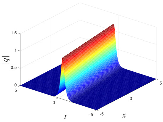
Figure 1. One-soliton solution (64) with ${\alpha }_1=0.7$, ${\eta }_1=0.6$.

When $N=2$, $q\left[0\right]=0$ and the spectral parameter ${\lambda }_2={\alpha }_2+i{\eta }_2$, we obtain a two-soliton solution of Equation (27)

$$\begin{array}{cc}\hfill q\left[2\right]=& -2{\eta }_1{e}^{2i{Y}_1}sech\left(2X_1\right)-4{\eta }_2\frac{M_1{M}_2{e}^{-2i{Y}_2}-{\alpha }_1{M}_{1}sech\left(2X_1\right)e^{2X_2-2i{Y}_1}}{{\left|M_1\right|}^2{e}^{2X_2}+{\left|M_2\right|}^2{e}^{-2X_2}+M_4+M_5+M_6}\hfill \\ \hfill & +4{\eta }_2\frac{i{\eta }_1{M}_{2}sech\left(2X_1\right)e^{-2X_2-2i{Y}_1}-M_3}{{\left|M_1\right|}^2{e}^{2X_2}+{\left|M_2\right|}^2{e}^{-2X_2}+M_4+M_5+M_6},\hfill \end{array}$$

(65)

where

$$\begin{array}{cc}& M_1={\alpha }_2-{\alpha }_{1}tanh\left(2X_1\right)+\left({\eta }_2-{\eta }_1\right)i,\hfill \\ & M_2={\alpha }_2-{\alpha }_1+\left({\eta }_2-{\eta }_{1}tanh\left(2X_1\right)\right)i,\hfill \\ & M_3=i{\alpha }_1{\eta }_1{sech}^2\left(2X_1\right)e^{-4i{Y}_1+2i{Y}_2},\hfill \\ & M_4=2isech\left(2X_1\right)sinh\left(2i{Y}_1-2i{Y}_2\right)\left({\eta }_1{\alpha }_2+{\alpha }_1{\eta }_2\right),\hfill \\ & M_5=2sech\left(2X_1\right)cosh\left(2i{Y}_1-2i{Y}_2\right)\left({\eta }_1{\eta }_2-{\eta }_1^2+{\alpha }_1{\alpha }_2-{\alpha }_1^2\right),\hfill \\ & M_6={sech}^2\left(2X_1\right)\left({\eta }_1^2{e}^{-2X_2}+{\alpha }_1^2{e}^{2X_2}\right),\hfill \\ & X_2=4{\alpha }_2{\eta }_{2}x+16\left({\alpha }_2^3{\eta }_2-{\alpha }_2{\eta }_2^3\right)t,\hfill \\ & Y_2=-2\left({\alpha }_2^2-{\eta }_2^2\right)x-4\left({\alpha }_2^2-6{\alpha }_2^2{\eta }_2^2\right)t.\hfill \end{array}$$

Case II: Taking $\mathbb{T}\times \mathbb{X}=\mathbb{R}\times \mathbb{C}$, we find

$$\begin{array}{cc}\hfill & \mu \left(t\right)=0,\hfill \\ \hfill & \nu \left(x\right)=\left\{\begin{array}{c}\hfill \frac{1}{3^{m+1}},x\in \mathbb{L},\\ \hfill 0,x\in \mathbb{C}\backslash \mathbb{L},\end{array}\right.\hfill \end{array}$$

(66)

where $\mathbb{C}$ is a Cantor set. $\mathbb{L}$ contains left discrete elements of $\mathbb{C}$,

$$\mathbb{L}=\left\{\sum _{k=1}^m\frac{a_k}{3^k}+\frac{1}{3^{m+1}}:m\in N,a_k\in \{0,2\},1\le k\le m\right\}.$$

Then, an N-fold DT of the GI equation is constructed

$$\begin{array}{cc}\hfill \psi \left[N\right]& =T\left[N\right]\psi [N-1]\hfill \\ \hfill & =(\lambda I-S[N-1\left]\right)\psi [N-1]\hfill \\ \hfill & =\left(\begin{array}{cc}\lambda -s_{11}[N-1]& -s_{12}[N-1]\\ -s_{21}[N-1]& \lambda -s_{22}[N-1]\end{array}\right)\psi [N-1]\hfill \\ \hfill & =T\left[N\right]\cdots T\left[3\right]T\left[2\right]T\left[1\right]\psi \left[0\right],\hfill \\ \hfill q\left[N\right]& =\left\{\begin{array}{c}q\left[0\right]+i\sum _{j=1}^N\frac{\left({\lambda }_j-{\lambda }_j^{*}\right){\psi }_1[j-1]{\psi }_2^{*}[j-1]}{{\left|{\psi }_1[j-1]\right|}^2+{\left|{\psi }_2[j-1]\right|}^2}+i\sum _{j=1}^N\frac{\left({\lambda }_j-{\lambda }_j^{*}\right){\psi }_1^{\rho }[j-1]{\psi }_2^{*\rho }[j-1]}{{\left|{\psi }_1^{\rho }[j-1]\right|}^2+{\left|{\psi }_2^{\rho }[j-1]\right|}^2},x\in \mathbb{L},t\in \mathbb{R},\hfill \\ q\left[0\right]+2i\sum _{j=1}^N\frac{\left({\lambda }_j-{\lambda }_j^{*}\right){\psi }_1[j-1]{\psi }_2^{*}[j-1]}{{\left|{\psi }_1[j-1]\right|}^2+{\left|{\psi }_2[j-1]\right|}^2},x\in \mathbb{C}\backslash \mathbb{L},t\in \mathbb{R}.\hfill \end{array}\right.\hfill \end{array}$$

(67)

According to Definition 3, we have

$$\begin{array}{c}\hfill e_{\pm 2i{\lambda }_1^4}(x,0)={\left[\frac{1\pm \frac{i{\lambda }_1^4}{3^{m+1}}}{1\mp \frac{i{\lambda }_1^4}{3^{m+1}}}\right]}^{\frac{x}{3^{m+1}}},e_{\pm i{\lambda }_1^2}(x,0)={\left[\frac{1\pm \frac{i{\lambda }_1^2}{2\times 3^{m+1}}}{1\mp \frac{i{\lambda }_1^2}{2\times 3^{m+1}}}\right]}^{\frac{x}{3^{m+1}}}.\end{array}$$

When $N=1$, $q\left[0\right]=0$ and the spectral parameter ${\lambda }_1={\alpha }_1+i{\eta }_1$, a one-soliton solution is obtained

$$q\left[1\right]=\left\{\begin{array}{c}\frac{1}{N_1}-\frac{{\left(3^{m+1}-i{\alpha }_1^2\right)}^2{M}_7-{\left(i{\eta }_1^2-2{\alpha }_1{\eta }_1\right)}^2{M}_7}{\left(i{\alpha }_1^2-i{\eta }_1^2\right)N_2},x\in \mathbb{L},t\in \mathbb{R},\hfill \\ -2{\eta }_1{e}^{2i{Y}_1}sech\left(2X_1\right),x\in \mathbb{C}\backslash \mathbb{L},t\in \mathbb{R},\hfill \end{array}\right.$$

(68)

where

$$\begin{array}{cc}& N_1={\left.E_1\right|}_{{\lambda }_1={\alpha }_1+i{\eta }_1}+{\left.E_2\right|}_{{\lambda }_1={\alpha }_1+i{\eta }_1},\hfill \\ & N_2={\left.E_1\right|}_{{\lambda }_1={\alpha }_1+i{\eta }_1}-{\left.E_2\right|}_{{\lambda }_1={\alpha }_1+i{\eta }_1},\hfill \\ & M_7=2{\eta }_1{\left[1+\frac{i{\alpha }_1^2}{3^{m+1}}\left(2i{\eta }_1^2-2i{\alpha }_1^2\right)\right]}^{3^{m+1}x}{e}^{\left(24i{\alpha }_1^2{\eta }_1^2-4i{\alpha }_1^4\right)t}.\hfill \end{array}$$

Case III: Taking $\mathbb{T}\times \mathbb{X}=\mathbb{R}\times {\mathbb{K}}_p$, we find

$$\begin{array}{c}\mu \left(t\right)=0,\hfill \\ \nu \left(x\right)=\left\{\begin{array}{c}(1-p^{-1})x,x=p^k\in p^{\mathbb{Z}},\hfill \\ 0,x=0,\hfill \end{array}\right.\hfill \end{array}$$

(69)

where $p>1$, $p^{\mathbb{Z}}=\left\{p^k:k\in \mathbb{Z}\right\}$ and ${\mathbb{K}}_p=p^{\mathbb{Z}}\bigcup \left\{0\right\}$.

Then, an N-fold DT is constructed

$$\begin{array}{cc}\hfill \psi \left[N\right]& =T\left[N\right]\psi [N-1]\hfill \\ \hfill & =(\lambda I-S[N-1\left]\right)\psi [N-1]\hfill \\ \hfill & =\left(\begin{array}{cc}\lambda -s_{11}[N-1]& -s_{12}[N-1]\\ -s_{21}[N-1]& \lambda -s_{22}[N-1]\end{array}\right)\psi [N-1]\hfill \\ \hfill & =T\left[N\right]\cdots T\left[3\right]T\left[2\right]T\left[1\right]\psi \left[0\right],\hfill \\ \hfill q\left[N\right]& =\left\{\begin{array}{c}q\left[0\right]+i\sum _{j=1}^N\frac{\left({\lambda }_j-{\lambda }_j^{*}\right){\psi }_1[j-1]{\psi }_2^{*}[j-1]}{{\left|{\psi }_1[j-1]\right|}^2+{\left|{\psi }_2[j-1]\right|}^2}+i\sum _{j=1}^N\frac{\left({\lambda }_j-{\lambda }_j^{*}\right){\psi }_1^{\rho }[j-1]{\psi }_2^{*\rho }[j-1]}{{\left|{\psi }_1^{\rho }[j-1]\right|}^2+{\left|{\psi }_2^{\rho }[j-1]\right|}^2},x\in p^{\mathbb{Z}},t\in \mathbb{R},\hfill \\ q\left[0\right]+2i\sum _{j=1}^N\frac{\left({\lambda }_j-{\lambda }_j^{*}\right){\psi }_1[j-1]{\psi }_2^{*}[j-1]}{{\left|{\psi }_1[j-1]\right|}^2+{\left|{\psi }_2[j-1]\right|}^2},x=0,t\in \mathbb{R}.\hfill \end{array}\right.\hfill \end{array}$$

(70)

According to

$$\begin{array}{cc}& {\int }_a^{b}f\left(x\right)\nabla x=\left(1-p^{-1}\right)\sum _{x=a}^{b}xf\left(x\right),\hfill \\ & {\int }_a^{b}f\left(\rho \left(x\right)\right)\nabla x=(p-1)\sum _{x=a}^{b}xf\left(x\right),\hfill \end{array}$$

we have

$$\begin{array}{cc}& e_{\pm i{\lambda }_1^2}(x,0)=e^{\left(1-p^{-1}\right)\sum _{x=0}^{p^k}\pm i{\lambda }_1^2},\hfill \\ & e_{\pm i{\lambda }_1^2}(\rho \left(x\right),0)=e^{(p-1)\sum _{x=0}^{p^k}\pm i{\lambda }_1^2}.\hfill \end{array}$$

When $N=1$, $q\left[0\right]=0$ and the spectral parameter ${\lambda }_1={\alpha }_1+i{\eta }_1$, a one-soliton solution is obtained

$$q\left[1\right]=\left\{\begin{array}{c}-{\eta }_1{e}^{\left(16{\alpha }_1{\eta }_1^3-16{\alpha }_1^3{\eta }_1-4i{\alpha }_1^4+24i{\alpha }_1^2{\eta }_1^2\right)t}{M}_8,x\in p^{\mathbb{Z}},t\in \mathbb{R},\hfill \\ -2{\eta }_1{e}^{2i{Y}_1}sech\left(2X_1\right),x=0,t\in \mathbb{R},\hfill \end{array}\right.$$

(71)

where

$$\begin{array}{cc}\hfill M_8=& e^{\left(1-p^{-1}\right)\sum _{x=0}^{p^k}\left(-2i{\alpha }_1^2+2i{\eta }_1^2\right)x}sech\left(1-p^{-1}\right)\sum _{x=0}^{p^k}4{\alpha }_1{\eta }_{1}x\hfill \\ \hfill & +e^{(p-1)\sum _{k=0}^{p^k}\left(-2i{\alpha }_1^2+2i{\eta }_1^2\right)x}sech\left(p-1\right)\sum _{x=0}^{p^k}4{\alpha }_1{\eta }_{1}x.\hfill \end{array}$$

4. Conclusions

In this paper, the coupled GI equation on a time–space scale was obtained by extending the Lax matrix equation on a time–space scale, which can be reduced to the classical GI equation. In particular, the semi-discrete GI equation was given by providing parallel computations for the discrete and continuous case. The standard DT of the GI equation was extended on a time–space scale. On this basis, its N-soliton solutions on a time–space scale were obtained, which were expressed using Cayley exponential functions.

The extension provides a wider range of nonlinear integrable dynamic models and promotes the study of nonlinear dynamic systems. By taking the “seed solution” $q=0$ and $\lambda =\alpha +i\beta$, one-solition solutions of the GI equation were obtained on three different time–space scales ( $\mathbb{X}$ = $\mathbb{R}$, $\mathbb{X}$ = $\mathbb{C}$ and $\mathbb{X}$ = $\mathbb{K}p$ ). In one case, the exact solution (64) and its dynamic figure were obtained when $x\in \mathbb{R}$. In the other cases, when $x\in \mathbb{C}\backslash \mathbb{L}$ and $x=0$, exact solutions (68) and (71) were obtained and were similar to Equation (64). However, when $x\in \mathbb{L}$ and $x\in p^{\mathbb{Z}}$, the structures of solutions (68) and (71) were more complicated and their values were different from those of Equation (64) at those discontinuity points.

Due to the limitations of the computer, it was difficult to obtain their dynamic figures at this stage. Furthermore, there is another well-known equation, the Eckhaus equation, which possesses a very similar structure. The Eckhaus equation is also integrable and has soliton-like solutions expressed in terms of the hyperbolic functions [37,38]. Therefore, we will find the most effective way to reduce structures of solutions (68) and (71) on $\mathbb{C}$ and $\mathbb{K}p$, and study the Eckhaus equation on a time–space scale in our future work.

References

- Hilger, S. Analysis on Measure Chains-A Unified Approach to Continuous and Discrete Calculus. Results Math. 1990, 18, 18–56. [Google Scholar] [CrossRef]
- Bohner, M.; Peterson, A. Advances in Dynamic Equations on a Time Scale; Birkhauser: Boston, MA, USA, 2003. [Google Scholar]
- Bohner, M.; Peterson, A. Dynamic Equations on a Time Scale: An Introduction with Applications; Springer Science and Business Media: Berlin, Germany, 2012. [Google Scholar]
- Meng, H.; Wang, L. Multiple periodic solutions in shifts δ ± for an impulsive functional dynamic equation on time scales. Adv. Differ. Equ. 2014, 152, 1–52. [Google Scholar]
- Agarwal, R.P.; Bohner, M.; Peterson, A. Dynamic equations on time scales: A survey. J. Comput. Appl. Math. 2002, 141, 1–26. [Google Scholar] [CrossRef]
- Saker, S.H. Oscillation of nonlinear dynamic equations on time scales. Appl. Math. Comput. 2004, 148, 81–91. [Google Scholar] [CrossRef]
- Kosmatov, N. Multi-point boundary value problems on time scales at resonance. J. Math. Anal. Appl. 2006, 323, 253–266. [Google Scholar] [CrossRef][Green Version]
- Anderson, D.R. Eigenvalue intervals for a two-point boundary value problem on a measure chain. J. Comput. Appl. Math. 2002, 141, 57–64. [Google Scholar] [CrossRef]
- Christiansen, F.B.; Fenchel, T.M. Theories of Populations in Biological Communities, volume 20 of Lecture Notes in Ecological Studies; Springer: Berlin, Germany, 1997. [Google Scholar]
- Andreasen, V. Multiple Time Scales in the Dynamics of Infectious Diseases; Springer: Berlin/Heidelberg, Germany, 1978. [Google Scholar]
- Bowman, C.; Gumel, A.B.; Dricssche, P. A mathematical model for assessing control strategies against West Nile virus. Bull. Math. Biol. 2005, 67, 1107–1133. [Google Scholar] [CrossRef] [PubMed]
- Atici, F.M.; Biles, D.C.; Lebedinsky, A. An application of time scales to economics. Math. Comput. Model. 2006, 43, 718–726. [Google Scholar] [CrossRef]
- Dryl, M.; Torres, D. A General Delta-Nabla Calculus of Variations on Time Scales with Application to Economics. Int. J. Dyn. Syst. Differ. 2014, 5, 42–71. [Google Scholar] [CrossRef]
- Hovhannisyan, G. Ablowitz–Ladik hierarchy of integrable equations on a time–space scale. J. Appl. Phys. 2014, 55, 102701. [Google Scholar] [CrossRef]
- Hovhannisyan, G.; Bonecutter, L.; Mizer, A. On Burgers equation on a time–space scale. Adv. Differ. Equ. 2015, 289, 1–19. [Google Scholar] [CrossRef]
- Cieslinski, J.L.; Nikiciuk, T.; Wakiewicz, K. The sine-Gordon equation on time scales. J. Math. Anal. Appl. 2015, 423, 1219–1230. [Google Scholar] [CrossRef]
- Cieslinski, J.L. Pseudospherical surfaces on time scales: A geometric definition and the spectral approach. J. Phys. A-Math. Theor. 2007, 40, 12525–12538. [Google Scholar] [CrossRef][Green Version]
- Cieslinski, J.L. New definitions of exponential, hyperbolic and trigonometric functions on time scales. J. Math. Anal. Appl. 2012, 388, 8–22. [Google Scholar] [CrossRef]
- Clarkson, P.A.; Tuszynski, J.A. Exact solutions of the multidimensional derivative nonlinear Schrodinger equation for many-body systems of criticality. J. Phys. A 1990, 23, 4269. [Google Scholar] [CrossRef]
- Hisakado, M.; Wadati, M. Integrable MultiComponent Hybrid Nonlinear Schrödinger Equations. J. Phys. Soc. Jap. 1995, 64, 408–413. [Google Scholar] [CrossRef]
- Kaup, D.J.; Newell, A.C. An exact solution for a derivative nonlinear Schrödinger equation. J. Math. Phys. 1978, 19, 798–801. [Google Scholar] [CrossRef]
- Xu, S.; He, J.; Wang, L. The Darboux transformation of the derivative nonlinear Schrödinger equation. J. Phys. A 2011, 44, 6629–6636. [Google Scholar] [CrossRef]
- Chen, H.H.; Lee, Y.C.; Liu, C.S. Integrability of Nonlinear Hamiltonian Systems by Inverse Scattering Method. Phys. Scr. 2007, 20, 490. [Google Scholar] [CrossRef]
- Ren, H.Y.; Li, D.S. Self-adjointness and Conservation Laws of Chen-Lee-Liu Equation. J. Pingdingshan Univ. 2013, 28, 14–17. [Google Scholar]
- Gerdjikov, V.S.; Ivanov, M.I. The quadratic bundle of general form and the nonlinear evolution equations. Bulg. J. Phys. 1983, 10, 35. [Google Scholar]
- Fan, E.G. Darboux transformation and soliton-like solutions for the Gerdjikov–Ivanov equation. J. Phys. A 2000, 33, 6925. [Google Scholar] [CrossRef]
- Gerdjikov, V.S.; Ivanov, M.I. A quadratic pencil of general type and nonlinear evolution equations. II. Hierarchies of Hamiltonian structures. Bulg. J. Phys. 1983, 10, 130–143. [Google Scholar]
- Pei, L.; Li, B. The Darboux transformation of the Gerdjikov–Ivanov equation from non-zero seed. In Proceedings of the 2011 International Conference on Consumer Electronics, Communications and Networks (CECNet), Xianning, China, 16–18 April 2011; pp. 5320–5323. [Google Scholar]
- Guo, L.; Zhang, Y.; Xu, S. The higher order Rogu’e Wave solutions of the Gerdjikov–Ivanov equation. Phys. Scr. 2014, 89, 240. [Google Scholar] [CrossRef]
- Dai, H.H.; Fan, E.G. Variable separation and algebro-geometric solutions of the Gerdjikov–Ivanov equation. Chaos Soliton. Fract. 2004, 22, 93–101. [Google Scholar] [CrossRef]
- Arshed, S. Two Reliable Techniques for the Soliton Solutions of Perturbed Gerdjikov–Ivanov Equation. Optik 2018, 33, 6925. [Google Scholar] [CrossRef]
- Nematollah, K.; Hossein, J. Analytical solutions of the Gerdjikov–Ivanov equation by using exp(ϕ(ξ))-expansion method. Optik 2017, 139, 72–76. [Google Scholar]
- Cao, C.; Geng, X.; Wang, H. Algebro-geometric solution of the 2+1 dimensional Burgers equation with a discrete variable. J. Math. Phys. 2002, 43, 621–643. [Google Scholar] [CrossRef]
- Saburo, K.; Tetsuya, K. Solutions of a derivative nonlinear schrödinger hierarchy and its similarity reduction. Glasgow Math. J. 2005, 47, 99–107. [Google Scholar] [CrossRef]
- Fan, E.G. Integrable evolution systems based on Gerdjikov–Ivanov equations, bi-Hamiltonian structure, finite-dimensional integrable systems and N-fold Darboux transformation. J. Math. Phys. 2000, 41, 7769–7782. [Google Scholar] [CrossRef]
- Fan, E.G. Bi-Hamiltonian Structure and Liouville Integrability for a Gerdjikov–Ivanov Equation Hierarchy. Chinese Phys. Lett. 2001, 18, 1. [Google Scholar]
- Cherniha, R. Galilean-invariant Nonlinear PDEs and their Exact Solutions. J. Nonlinear Math. Phys. 1995, 2, 374–383. [Google Scholar] [CrossRef]
- Calogero, F.; Lillo, S.D. The Eckhaus PDE iψt + ψxx + 2(|ψ|2)xψ + |ψ|4ψ = 0. Inverse Probl. 1999, 3, 633. [Google Scholar] [CrossRef]
Publisher’s Note: MDPI stays neutral with regard to jurisdictional claims in published maps and institutional affiliations. |
© 2021 by the authors. Licensee MDPI, Basel, Switzerland. This article is an open access article distributed under the terms and conditions of the Creative Commons Attribution (CC BY) license (https://creativecommons.org/licenses/by/4.0/).