Effects of Charged Solute-Solvent Interaction on Reservoir Temperature during Subsurface CO₂ Injection

Abstract

A short-term side-effect of CO₂ injection is a developing low-pH front that forms ahead of the bulk water injectant, due to differences in solute diffusivity. Observations of downhole well temperature show a reduction in aqueous-phase temperature with the arrival of a low-pH front, followed by a gradual rise in temperature upon the arrival of a high concentration of bicarbonate ion. In this work, we model aqueous-phase transient heat advection and diffusion, with the volumetric energy generation rate computed from solute-solvent interaction using the Helgeson–Kirkham–Flowers (HKF) model, which is based on the Born Solvation model, for computing specific molar heat capacity and the enthalpy of charged electrolytes. A computed injectant water temperature profile is shown to agree with the actual bottom hole sampled temperature acquired from sensors. The modeling of aqueous-phase temperature during subsurface injection simulation is important for the accurate modeling of mineral dissolution and precipitation because forward dissolution rates are governed by a temperature-dependent Arrhenius model.

1. Introduction

The first geologic carbon sequestration test in the United States was the Frio Brine Pilot experiment funded by the Department of Energy (DOE) National Energy Technology Laboratory (NETL) under the leadership of the Bureau of Economic Geology (BEG) at the Jackson School of Geosciences, The University of Texas at Austin, with major collaboration from the GEO-SEQ project, a national lab consortium led by Lawrence Berkeley National Laboratory (LBNL) [1]. In this test, 1600 metric tons of CO₂ was injected into a sandstone layer residing in the Frio Formation, located east of Houston, Texas. An injection well was drilled to 1750 m KB (5755 ft KB) and perforated in the upper part of the upper Frio C sandstone region. An existing well 100 ft (30 m) updip was used as an observation well for measuring temperature, pressure, and solute concentration. Table 1 shows the depth of each region. The examination of water samples taken from the observation well over the span of one month, in which injection took place over a 10-day period, revealed a decrease in pH (from 6.5 to 5.7) occurred well before the arrival of fluid with increased alkalinity (from 100 to 3000 mg/L as HCO₃⁻ [2]. A major concern of this finding was the potential for the rapid dissolution of carbonate minerals that encounter the acidic front, which could lead to undesirable increased permeability in rock seals or well cements and the subsequent potential leakage of CO₂ and brine. On the other hand, an advancing low pH front may increase the wettability of mineral surfaces, which would improve CO₂ sequestration efficiency with respect to the capillarity of the moving effluent, as well as aid in enhanced oil recovery operations. Previous research by Pruess and Müller [3] showed, through 1D numerical simulation, that the injection of CO₂ into saline aquifers may cause formation dry-out and the precipitation of NaCl_(s) near an injection well and that such precipitation would reduce formation porosity, permeability, and injectivity, leading to a pressure build up. While Pruess and Müller’s simulations were isothermal, they concluded that nonisothermal effects could result in greater effects on reducing formation porosity, permeability, and injectivity if CO_2(g) is injected at a temperature different from the formation aqueous brine phase. In subsequent research, Pruess derived [4] an analytical expression for finding the saturation of NaCl_(s) (i.e., the volume fraction of solid NaCl precipitate) in the dry-out region.

Table 1. The shale, sandstone, and perforation regions of the injection and observation wells.

Zone	Injection Well (ft, m)	Observation Well (ft, m)
Top “A” sandstone
Top “B” Shale
Top “B” Sandstone	−4966, −1514	−4938, −1505
Top “C” shale	−4978, −1517	−4950, −1509
Top “C” sandstone	−5034, −1534	−5000, −1524
Top Perforation		−5014, −1528
Bottom Perforation		−5034, −1534
Bottom “C” sandstone

1.1. Separation Distance between the Diffusive Acidic and Alkaline Bulk Effluent Fronts

1D numerical simulations were conducted to examine the distance between the developing acidic front and the alkaline front as a function of reservoir temperature, seepage velocity, and time [5]. Figure 1 shows the separation distance as a function of seepage velocity and reservoir temperature after 5 years computed using a 1D reaction transport modeling (RTM) application [6] configured for a sandstone lithology similar to the high-permeability brine-bearing sandstone of the Frio Formation. A substantial contributing factor to the development of a low pH front is the order of magnitude difference in solute diffusivity (see Table 2) between hydron H⁺ (1.4770 × 10⁻⁴ cm² s⁻¹) and bicarbonate ion HCO₃⁻ (2.1560 × 10⁻⁵ cm² s⁻¹), as approximated using the model of Boudreau in Equation (1) [7], with the parameters T_c and T_f representing the solutes used in a 1D reaction transport application to model the diffusion and sweep front distance given in Figure 1. A superimposed plot of the observation-well-sampled temperature and pressure measurements [8] for the month of October 2004 is shown in Figure 2. The vertical green line in the figure denotes the arrival of an introduced gas-phase fluorescent tracer to indicate CO₂ breakthrough. The three pressure drop shown in the figure identifies the pump shutoff. The data show an initial, pre-injection reservoir temperature of 58.4 °C and a final post-injection temperature of 58.8 °C at the final 30-day sampling, with a remarkable drop in temperature to 57.6 °C at breakthrough. One may suspect the sharp temperature drop is a result of Joule–Thomson cooling, but the Joule–Thomson coefficient μ_JT has been shown to be positive for pure CO₂ at several reservoir representative temperatures across a pressure range of 1 to 500 bar [9],

$$D={10}^{-6}\left(T_c+T_{f}T\right),\left[c{m}^2{s}^{-1}\right]$$

(1)

$${\mu }_{JT}={\left(\frac{\partial T}{\partial P}\right)}_H\approx \frac{\Delta T}{\Delta P}$$

(2)

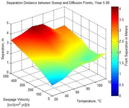
Figure 1. The separation distance between the low pH diffusion front and the high alkalinity sweep front as a function of seepage velocity, reservoir temperature, and time.

Table 2. The model parameters and diffusion coefficient values D computed at T = 65 °C using the model of Boudreau [7].

	H+	OH−	SiO2(aq)	K+	CO2(aq)	HCO3−	CO3−2	Na+	Al(OH)3(aq)	Ca+2	Fe+2	Mg+2
Tc	54.40	25.90	5.00	9.55	5.50	5.06	4.33	6.06	4.46	3.60	3.31	3.43
Tf	1.555	1.094	0.500	0.409	0.325	0.275	0.199	0.297	0.243	0.179	0.150	0.144
D	1.6 × 10−4	9.7 × 10−5	3.8 × 10−5	3.6 × 10−5	2.7 × 10−5	2.3 × 10−5	1.7 × 10−5	2.5 × 10−5	2.0 × 10−5	1.5 × 10−5	1.3 × 10−5	1.3 × 10−5

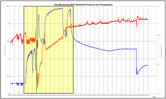
Figure 2. The observation well bottom hole pressure and temperature measurements during the month of October 2004. The injection period is represented by the yellow highlight. The breakthrough time is represented by the green vertical line.

And the corresponding drop in temperature occurs with an increase in pressure at breakthrough.

1.2. Contribution of Soulte-Solute Interaction on Temperature

In this paper we show, using numerical 3D reaction transport modeling, how the interaction of charged electrolytes with the formation water solvent produces a temperature profile in agreement with sampled wellbore measurements. The results of numerical simulation also show the arrival of the low pH diffusion front results in relative cooling, while the later arrival of the high alkalinity sweep front results in a steady temperature increase and the maintenance of a relatively heated plume that approaches 58.8 °C for 17 days post-injection up to the 30-day final measurement, due to a calculated aqueous-phase thermal diffusivity α of approximately 4 × 10⁻⁷ m² s⁻¹. To model the temperature change resulting from the charged solute-solvent interaction, we implemented the Helgeson–Kirkham–Flowers (HKF) model [10], which is based on the Born solvation model [11,12] that governs the aqueous-phase thermodynamics of the ion–solvent interaction, within an existing RTM application [6] that was extended to 3D with new numerical models, developed by the author, for poroelasticity, thermal transport, and porous media flow. The modeling of the aqueous-phase temperature during the simulation of the subsurface injection is important for the accurate modeling of mineral dissolution and precipitation because forward dissolution rates are governed by the temperature-dependent Arrhenius model.

1.3. Organization of This Article

The remainder of this article is organized as follows. Nomenclature provides a table of definitions of symbols used throughout this document. Section 2.1, The Born Solvation Model, provides a theoretical background of the model used to find the change in free energy due to solvation. Section 2.2, Aqueous Phase Thermal Transport, discusses the construction of the source term used in an advection–diffusion model to simulate thermal transport and a discussion of the finite element method (FEM) used to implement the model. Section 2.4, Porous Media Flow, discusses coupled models used to simulate fluid velocity and density in brine saturated sandstone. Section 2.7, Poroelastic Model, discusses coupled models used to simulate shale and sandstone strain, stress, and porosity. Section 2.9, Aqueous Phase Mass Transport, discusses the advection–diffusion reaction model to simulate solute (mass) transport and the kinetic mechanism used to model mineral dissolution and precipitation. Section 2.11, Frio Formation Simulated Configuration, presents the design of a new software application developed to simulate subsurface CO₂ injection and how the application was configured to simulate CO₂ injection into the Frio Formation. Section 3, Results and Discussion, presents results of simulating CO₂ injection into the Frio Formation with respect to a developing temperature gradient between the acidic and alkaline fronts. Section 4, Conclusions, summarizes the major findings of this paper.

2. Methodology

2.1. The Born Solvation Model

The electric field of a charged electrolyte (ion) solute will interact with the dipoles that form a water solvent. The permittivity (dielectric constant) ε of the water solvent determines how the ion’s applied electric field affects charge migration (electric flux) and dipole reorientation in the solvent. The Born model provides an approximation of the standard state molar Gibbs free energy of solvation, $\Delta {\overline{G}}_s^{\circ }$ which works by establishing a polarization charge in a solvent upon the introduction of an ion. The permittivity ε is a measure of capacitance that is encountered by an ion when forming an electric field in a medium, such as the reservoir formation water, and describes the amount of charge needed to generate one unit of electric flux in a given medium. In our RTM application, calculations for the relative permittivity of H₂O use the power series Equation (3) and parameters (Table 3) generated by Johnson and Norton [13],

$${\epsilon }_r={\displaystyle \sum _{k=1}^5{c}_k{D}_w^{k-1}},\mathrm{where}{c}_1=1,c_2=\frac{a_1}{T_n},c_3=\frac{a_2}{T_n}+a_3+a_4{T}_n,c_4=\frac{a_5}{T_n}+a_6{T}_n+a_7{T}_n^2,c_5=\frac{a_8}{T_n^2}+\frac{a_9}{T_n}+a_{10}$$

(3)

Table 3. The regression parameters for Equation (3) from Johnson and Norton [13].

a1	a2	a3	a4	a5
0.1470333593 × 102	0.2128462733 × 103	−0.1154445173 × 103	0.1955210915 × 102	−0.8330347980 × 102
a6	a7	a8	a9	a10
0.3213240048 × 102	−0.6694098645 × 101	−0.3786202045 × 102	0.6887359646 × 102	−0.2729401652 × 102

An ion’s charge will yield more electric flux in a solvent with low permittivity than in a solvent with high permittivity. From Equation (3), the relative permittivity of H₂O decreases with increasing temperature. At lower temperatures, H₂O dipoles can become more aligned and establish a polarization charge, while at higher temperatures the dipoles are less able to align due to random molecular motion from increased kinetic energy, which results in more flux or charge migration through the solvent [14]. From Coulomb’s Law, the force on a test charge Q due to a single point charge q (at rest) a distance r apart is

$$F=\frac{1}{4\pi {\epsilon }_r{\epsilon }_0}\frac{qQ}{r^2}\widehat{r},\frac{N{m}^2}{C^2}\frac{C^2}{m^2}=Nr$$

(4)

From (4), the electric potential from a point charge q at a distance r from q is given by

$$\varphi \left(r\right)=\frac{q}{4\pi {\epsilon }_r{\epsilon }_{0}r},\frac{{\mathrm{N}\mathrm{m}}^2}{{\mathrm{C}}^2}\frac{\mathrm{C}}{\mathrm{m}}=\frac{\mathrm{N}\mathrm{m}}{\mathrm{C}}=\frac{\mathrm{J}}{\mathrm{C}}=\mathrm{V}$$

(5)

And from (5), it follows that the electric potential from a uniform set of Z (i.e., valence) elementary charges e (coulombs) at a distance r from Ze is

$$\varphi \left(r\right)=\frac{Ze}{4\pi {\epsilon }_r{\epsilon }_{0}r},\mathrm{V}$$

(6)

The energy U of an electric field E from the successive introduction of point charges in a medium with absolute permittivity ε can be found by first assuming the energy from introducing the first point charge q₁ into an empty medium will give U_q1 = 0. From (5), the energies U_{q1, q2}, U_{q1, q2, q3}, and U_{q1, q2, q3,…, qn} from introducing the second, third, and nth point charges, respectively, are

$$U_{q_2}=\frac{1}{4\pi \epsilon }{q}_2\frac{q_1}{r_{1,2}},U_{q_3}=\frac{1}{4\pi \epsilon }{q}_3\left(\frac{q_1}{r_{1,3}}+\frac{q_2}{r_{2,3}}\right),\dots ,U_{q_n}=\frac{1}{4\pi \epsilon }\frac{1}{2}{\displaystyle \sum _{i=1}^n{\displaystyle \sum _{j\ne i}^n\frac{q_i{q}_j}{r_{i,j}}}}$$

(7)

In the last term of (7), a division by 2 is required since the product charges q_i q_j and q_j q_i are each counted [15]. Factoring the potential function (5) from (7), we have

$$U_{q_n}=\frac{1}{2}{\displaystyle \sum _{i=1}^n{q}_i\left({\displaystyle \sum _{j\ne i}^n\frac{1}{4\pi \epsilon }\frac{q_j}{r_{i,j}}}\right)}=\frac{1}{2}{\displaystyle \sum _{i=1}^n{q}_i\varphi \left({\overline{r}}_i\right)}$$

(8)

For a charge density ρ, integrating over an arbitrary volume V with permittivity ε, we have

$$U=\frac{1}{2}{\displaystyle \underset{V}{\iiint }\rho \varphi dV}=\frac{1}{2}{\displaystyle \underset{V}{\iiint }\left(\epsilon \nabla \cdot E\right)\varphi dV=}\frac{\epsilon }{2}\left[-{\displaystyle \underset{V}{\iiint }E\cdot \nabla \varphi dV+{\displaystyle \underset{S}{∯}\varphi E\cdot \widehat{n}dS}}\right]$$

(9)

where Gauss’s law ${\displaystyle \epsilon (\nabla ·E)=\rho }$ is employed in the second term and the product rule $\nabla ·(\varphi E)=\varphi (\nabla ·E)+E·\nabla \varphi$ and divergence theorem are employed in the third term. From the fundamental theorem of calculus for line integrals, ∇φ = −E, and observing as r →∞ where the electric potential at infinity is assumed to be zero [15],

$$S=4\pi r^2\to r^2,E=\frac{1}{4\pi \epsilon }\frac{q}{r^2}\widehat{r}\to \frac{1}{r^2},\varphi \left(r\right)=\frac{q}{4\pi {\epsilon }_r{\epsilon }_{0}r}\to \frac{1}{r}\Rightarrow {\displaystyle \underset{S}{∯}\varphi E\cdot ndS}\to \frac{1}{r}\to 0$$

(10)

Equation (9) reduces to

$$U=\frac{\epsilon }{2}{\displaystyle \underset{V}{\iiint }{\left|E\right|}^{2}dV}=\frac{{\epsilon }_0{\epsilon }_r}{2}{{\displaystyle \underset{V}{\iiint }\left|\frac{1}{4\pi {\epsilon }_0{\epsilon }_r}\frac{q}{r^2}\widehat{r}\right|}}^{2}dV=\frac{{\epsilon }_0{\epsilon }_r}{2}\frac{q^2}{16{\pi }^2{\left({\epsilon }_0{\epsilon }_r\right)}^2}{\displaystyle \underset{V}{\iiint }\frac{1}{r^4}}dV$$

(11)

For the energy of uniformly a charged spherical shell (ion) of total charge q and radius r. Substituting dV = dA dr = r²sinθdθdφ dr and q = Ze into (11) and integrating over the volume outside of the ion’s surface from r = r_i to r = ∞, where r_i is the radius of the ion, we obtain the Born expression [12] for the energy of an ion with charge Ze in a medium of permittivity ε,

$$\begin{array}{l}\frac{1}{2}\frac{{\epsilon }_r{\epsilon }_0{Z}^2{e}^2}{16{\pi }^2{\left({\epsilon }_r{\epsilon }_0\right)}^2}{\displaystyle \underset{V}{\iiint }{r}^2\frac{1}{r^6}dr}dA=\frac{1}{2}\frac{{\epsilon }_r{\epsilon }_0{Z}^2{e}^2}{16{\pi }^2{\left({\epsilon }_r{\epsilon }_0\right)}^2}{\displaystyle \underset{V}{\iiint }{r}^2\frac{1}{r^6}dr}{r}^{2}sin\theta d\theta d\varphi =\\ \frac{1}{2}\frac{{\epsilon }_r{\epsilon }_0{Z}^2{e}^2}{16{\pi }^2{\left({\epsilon }_r{\epsilon }_0\right)}^2}4\pi {\displaystyle \underset{r_i}{\overset{\infty }{\int }}\frac{1}{r^2}}dr=\frac{Z^2{e}^2}{8\pi \epsilon }\left[-\frac{1}{\infty }--\frac{1}{r_i}\right]=\frac{Z^2{e}^2}{8\pi \epsilon r_i}=k_e\frac{Z^2{e}^2}{2\epsilon r_i}\end{array}$$

(12)

Denoting U₀ as the energy of the electric field of an ion in a vacuum and U as the energy of the electric field of an ion in a medium (solvent) of relative permittivity ε_r, the energy difference U-U₀ provides the work done introducing an ion into a solvent, or equivalently, the Gibbs free energy of solvation,

$$\Delta G_s=U-U_0=k_e\frac{Z^2{e}^2}{2{\epsilon }_r{r}_i}-k_e\frac{Z^2{e}^2}{2r_i}=k_e\frac{Z^2{e}^2}{2r_i}\left(\frac{1}{{\epsilon }_r}-1\right)$$

(13)

Multiplying (13) by the Avogadro constant N_A and defining the absolute Born coefficient ${\omega }_j^{abs}$, the absolute standard molal Gibbs free energy of solvation of the j^th ion in a solvent is given by [14,16]

$${\Delta \overline{G}}_{s,j}^{\circ ,abs}=\frac{N_A{Z}_j^2{e}^2}{8\pi {\epsilon }_0{r}_j}\left(\frac{1}{{\epsilon }_r}-1\right)={\omega }_j^{abs}\left(\frac{1}{{\epsilon }_r}-1\right)$$

(14)

Substituting the effective ionic radius, $r_{e,j}=r_{j,T_r,P_r}+\left|Z_j\right|g\left(T,P\right)$, defined by Tanger and Helgeson [17], where r_j is the crystallographic ionic radius (~0.3Å to 2Å) and g is a solvent function at reference temperature and pressure with units of Å obtained by regression of and heat capacity and volume data for NaCl_aq [14,17,18]. To derive the thermodynamic properties, such as specific heat capacity and specific enthalpy, of charged solutes, which are needed in our thermal transport model, Tanger and Helgeson define a conventional electrostatic Born coefficient ω_j. The conventional coefficient is the difference between the absolute Born coefficient for ion j, which represents $\Delta {\overline{G}}_{s,j}^{°}$ of ion j, and $\Delta {\overline{G}}_{s,hs}^{°}$ which is the Gibbs free energy required to form an inner hydration sphere of H₂O dipoles encompassing ion j. The hydration sphere Gibbs free energy is the valence of ion j, Z_j,, multiplied by $\Delta {\overline{G}}_{s,H^{+}}^{°}$, the solvation energy for a proton. The conventional Born coefficient defined by Tanger and Helgeson is thus ${\omega }_j={\omega }_{j^{}}^{abs}-Z_j{\omega }_{H^{+}}^{abs}$, and the relative standard state molar Gibbs free energy of solvation of ion j becomes

$$\Delta {\overline{G}}^{\circ }{}_{s,j}={\omega }_j\left(\frac{1}{{\epsilon }_r}-1\right)$$

(15)

For ε_r > 1 in (15), $\Delta {\overline{G}}^{\circ }{}_{s,j}$< 0, which indicates the movement of an ion from a less polar solvent, such as a vacuum, to H₂O, is thermodynamically favorable. In addition, the magnitude of $\Delta {\overline{G}}_{s,j}^{°}$ decreases as the ionic radius r_j increases since the voltage φ(r) at the ion’s outer shell, defined by Equation (6), decreases with the distance from the ion’s center where all charge is assumed (by the Born model) to reside [19]. From (15), the standard state molar entropy of solvation is obtained through the relation

$$-{\left(\frac{\partial \Delta {\overline{G}}_s^{\circ }}{\partial T}\right)}_P=\Delta {\overline{S}}_s^{\circ }=-{\partial \left({\omega }_j\left(\frac{1}{{\epsilon }_r\left(T\right)}-1\right)\right)/\partial T|}_P=-{\omega }_j\left(-\frac{1}{{\epsilon }_r^2\left(T\right)}{\left(\frac{\partial {\epsilon }_r}{\partial T}\right)}_P\right)-\left(\frac{1}{{\epsilon }_r\left(T\right)}-1\right){\left(\frac{\partial {\omega }_j}{\partial T}\right)}_P$$

(16)

The standard state molar enthalpy of solvation is then found by substituting (16) into $\Delta {\overline{G}}_s^{°}=\Delta {\overline{H}}_s^{°}-T\Delta {\overline{S}}_s^{°}$,

$$\Delta {\overline{H}}_s^{\circ }=\Delta {\overline{G}}_s^{\circ }+T\Delta {\overline{S}}_s^{\circ }=\omega \left(\frac{1}{{\epsilon }_r}-1\right)+\omega TY-T\left(\frac{1}{{\epsilon }_r}-1\right){\left(\frac{\partial \omega }{\partial T}\right)}_P$$

(17)

where the partial derivatives of relative permittivity ε_r at constant pressure are denoted as functions Z, Y, and X [16],

$$Z=-\left(\frac{1}{{\epsilon }_r}\right),Y={\left(\frac{\partial Z}{\partial T}\right)}_P=\left(\frac{1}{{\epsilon }_r^2}\right){\left(\frac{\partial {\epsilon }_r}{\partial T}\right)}_P\left[\frac{1}{K}\right],X={\left(\frac{\partial Y}{\partial T}\right)}_P=\left(\frac{1}{{\epsilon }_r^2}\right){\left(\frac{{\partial }^2{\epsilon }_r}{\partial T^2}\right)}_P-\left(2{\epsilon }_r{Y}^2\right)\left[\frac{1}{K^2}\right]$$

(18)

For $\Delta {\overline{H}}_s^{°}$ < 0, the ion–solvent interaction is exothermic, and there will be a temperature increase in the formation water. The first and second partial derivatives of relative permittivity ε_r from Equation (3) at constant pressure are given by

$$\begin{array}{c}{\left(\frac{\partial {\epsilon }_r}{\partial T}\right)}_P={\displaystyle \sum _{j=0}^4{D}_w^j\left[{\left(\frac{dc}{dT}\right)}_{j+1}-j\alpha c_{j+1}\right]}\hfill \\ {\left(\frac{{\partial }^2{\epsilon }_r}{\partial T^2}\right)}_P={\displaystyle \sum _{j=0}^4{D}_w^j[{\left(\frac{d^{2}c}{d{T}^2}\right)}_{j+1}-j\left(\alpha {\left(\frac{dc}{dT}\right)}_{j+1}+c_{j+1}\frac{d\alpha }{dT}\right)-j\alpha ({\left(\frac{dc}{dT}\right)}_{j+1}-{j\alpha c}_{j+1})]}\hfill \end{array}$$

(19)

The first and second partial derivatives of the conventional Born coefficient ω_j are given by [16].

$$\begin{array}{l}\left(\frac{\partial \omega }{\partial T}\right)=-\eta X_1{\left(\frac{\partial g}{\partial T}\right)}_p\left[\frac{J}{\mathrm{mol}K}\right],X_1=\frac{abs(z^3)}{{(r_i)}^2}-\left[\frac{z}{{\left(3.082+g\right)}^2}\right]\hfill \\ \left(\frac{{\partial }^2\omega }{\partial T^2}\right)=2\eta X_2{\left(\frac{\partial g}{\partial T}\right)}^2{}_p-\eta X_1{\left(\frac{{\partial }^{2}g}{\partial T^2}\right)}_p\left[\frac{J}{\mathrm{mol}{K}^2}\right],X_2=\frac{abs(z^4)}{{(r_i)}^3}-\left[\frac{z}{{\left(3.082+g\right)}^3}\right]\hfill \end{array}$$

(20)

From (17), H.C. Helgeson, D.H. Kirkham, and G.C. Flowers (Helgeson et al., 1981), derived a revised model for specific molar heat capacity ${\overline{c}}_P$

$${\overline{c}}_P^{\circ }=\underset{\mathrm{nonsolvation}\mathrm{contribution}}{\underbrace{c_1+\frac{c_2}{{\left(T-\Theta \right)}^2}-\frac{2T}{{\left(T-\Theta \right)}^3}\left[a_3\left(P-P_r\right)+a_4\ln \left(\frac{\Psi +P}{\Psi +P_r}\right)\right]}}+\underset{\mathrm{solvation}\mathrm{contribution}}{\underbrace{\omega TX+2TY{\left(\frac{\partial \omega }{\partial T}\right)}_P-T\left(\frac{1}{{\epsilon }_r}-1\right){\left(\frac{{\partial }^2\omega }{\partial T^2}\right)}_P}}$$

(21)

and specific molar enthalpy $\overline{h}$ [14,16]

$$\begin{array}{l}{\overline{h}}^{\circ }=c_1\left(T-T_r\right)-c_2\left[\left(\frac{1}{T-\Theta }\right)-\left(\frac{1}{T_r-\Theta }\right)\right]+a_1\left(P-P_r\right)+a_2\ln \left(\frac{\Psi -P}{\Psi -P_r}\right)+\\ \left(\frac{2T-\Theta }{{\left(T-\Theta \right)}^2}\right)\left[a_3\left(P-P_r\right)+a_4\ln \left(\frac{\Psi +P}{\Psi +P_r}\right)\right]+\omega \left(\frac{1}{\epsilon }-1\right)+\omega TY-T\left(\frac{1}{\epsilon }-1\right){\left(\frac{\partial \omega }{\partial T}\right)}_P-\\ {\omega }_{\mathrm{Pr},Tr}\left(\frac{1}{{\epsilon }_{\mathrm{Pr},Tr}}-1\right)-{\omega }_{\mathrm{Pr},Tr}{T}_r{Y}_{\mathrm{Pr},Tr}\end{array}$$

(22)

For an aqueous electrolyte species j, in (22), coefficients a_i and c_i are species dependent non-solvent regression parameters ([20], p. 92).

2.2. Aqueous Phase Thermal Transport

The aqueous-phase volumetric energy generation rate S_T can be derived by summing, over all solutes j for n solutes, the rate of change of molar concentration of species j multiplied by that species’ specific molar enthalpy given by (22),

$$S_T={\displaystyle \sum _{j=1}^n\frac{d{c}_j}{dt}{\overline{h}}_j\left[\frac{J}{m^{3}s}\right]}$$

(23)

The transient heat advection–diffusion reaction model is then

$$\frac{\partial \left(\rho c_{p}T\right)}{\partial t}+\nabla \cdot \left(\rho c_{p}Tu\right)=\nabla \cdot \left(k\nabla T\right)+S_T$$

(24)

where u is fluid velocity, k = k(T) is the thermal conductivity of H₂O, and ρ = ρ(T) is the density of H₂O.

2.3. Transient Finite Element Method Formulation

A Crank–Nicolson discretization scheme is used with time step Δt and implemented using the deal.II general-purpose, object-oriented, finite element library [21]. A weak formulation with weight function v and solution wⁿ at time t_n is given by

$$\frac{1}{\Delta t}m(w^{n+1},v)+\frac{1}{2}a(t_{n+1},w^{n+1},v)=\frac{1}{\Delta t}m(w^n,v)+\frac{1}{2}a(t_n,w^n,v)+\frac{1}{2}\left(F(t_n;v)+F(t_{n+1};v)\right)$$

(25)

Functionals with thermal diffusivity α and a solute-solvent reaction thermal rate S_T/ρc_p with units K s⁻¹ are

$$\begin{array}{ccc}\hfill m(w,v)& =& {\displaystyle {\int }_{\Omega }w}vdV\hfill \\ \hfill a(t_n,w,v)& =& {\displaystyle {\int }_{\Omega }\alpha }\nabla w^n\cdot \nabla v+u(t_n)\cdot \left(\nabla w^n\right)v+\nabla \cdot u(t_n)w^{n}vdV\hfill \\ \hfill F(t,v)& =& {\displaystyle {\int }_{\Omega }\left(S_T/\rho c_p\right)}vdV\hfill \end{array}$$

(26)

For N_h node points, define the function u from Lagrange basis polynomials φ

$$u={\displaystyle \sum _{j=1}^{N_h}{u}_j}{\varphi }_j$$

(27)

Let Uⁿ ∈ R^Nh be the vector of coefficients u_j for the finite element solution at time step n. The aqueous-phase temperature at the n + 1^th time step is solved via the implicit system

$$\left(M+\frac{\Delta t}{2}A(t_{n+1})\right)U^{n+1}=\left(M+\frac{\Delta t}{2}A(t_n)\right)U^n+\frac{\Delta t}{2}(f_{n+1}+f_n)$$

(28)

where

$$\begin{array}{ccc}\hfill M_{ij}& =& m({\varphi }_i,{\varphi }_j)\hfill \\ A_{ij}(t_n)& =& a(t_n;{\varphi }_i,{\varphi }_j)\hfill \\ \hfill f_{n(i)}& =& F(t_n;{\varphi }_i)\hfill \end{array}$$

(29)

2.4. Porous Media Flow

A Darcy Law formulation for fluid flux is implemented to model aqueous-phase fluid injection,

$$v_{\mathrm{res}}=-\frac{K}{\mu }{\rho }_0\left(\nabla p_{\mathrm{res}}-{\rho }_{res}g\nabla z\right)$$

(30)

Equation (30) is solved simultaneously with the continuity Equation [22]

$${\partial }_t({\rho }_0{\varphi }^{*})+\nabla \cdot v_{\mathrm{res}}=q_{\mathrm{res}}$$

(31)

2.5. Mixed Finite Element Method Formulation

We use a mixed finite element method to simultaneously calculate the reservoir fluid velocity vector field v_res, together with a scalar reservoir pressure field p and test functions ψ and χ, respectively. A weak formulation is constructed by multiplying (30) by a vector valued function ψ and (31) by a scalar valued function χ and then integrating the domain Ω,

$${\displaystyle {\int }_{\Omega }{\psi }^T}\left(v_{res}+\frac{K{\rho }_0}{\mu }\left(\nabla p_{res}-{\rho }_{res}g\widehat{z}\right)\right)dV=0$$

(32)

$${\displaystyle {\int }_{\Omega }\chi }\left({\partial }_t\left({\rho }_0{\varphi }^{*}\right)+\nabla \cdot v_{res}-q_{res}\right)dV=0$$

(33)

For a given pair of test functions, (ψ, χ), (32) and (33) states that the weighted residual (error) of PDEs (30) and (31), when applied to solution functions v_res and p, will be zero. Equations (32) and (33) are a weak form of (30) and (31), respectively, because these weak-form equations may also be true for other test functions that would then approximate the so-called strong solutions that solve the original, strong form of the PDEs. The weak form equations can be rewritten with additive terms separated,

$${(\psi ,v_{res})}_{\Omega }+{\left(\psi ,\frac{K{\rho }_0}{\mu }\nabla p_{res}\right)}_{\Omega }-{\left(\psi ,\frac{K{\rho }_0}{\mu }{\rho }_{res}g\widehat{z}\right)}_{\Omega }=0$$

(34)

$${(\chi ,{\partial }_t({\rho }_0{\varphi }^{*}))}_{\Omega }+{(\chi ,\nabla \cdot v_{res})}_{\Omega }-{(\chi ,q_{res})}_{\Omega }=0$$

(35)

The pressure gradient term ∇p_res in (34) can be eliminated by applying the product rule and the Divergence Theorem,

$$\nabla \cdot \left(p_{res}\psi \right)=p_{res}\left(\nabla \cdot \psi \right)+\psi \cdot \nabla p_{res}$$

(36)

Applying the Divergence Theorem introduces an integral term in terms of the divergence of test function ψ, and a boundary integral in terms of the pressure values and the normal component of the test function, ψ · n. Normalizing (34) by multiplying each term by μ K⁻¹ ρ₀⁻¹ gives

$${(\psi ,\frac{\mu K^{-1}}{{\rho }_0}{v}_{res})}_{\Omega }+{⟨\psi \cdot n,p_{res}⟩}_{\partial \Omega }-{(\nabla \cdot \psi ,p_{res})}_{\Omega }-{(\psi ,{\rho }_{res}g\widehat{z})}_{\Omega }=0$$

(37)

To obtain a unique solution, a constraint is placed on the pressure function. In our model, the far field pressure on the boundary furthest from the injection location and above the caprock layer is given a Dirichlet boundary condition set to equal the initial pressure. The assumption is that the far field pressure is beyond the range of influence of the fluid injection. We call the portion of the boundary where this condition is set Γ_D, and we split the boundary integral as

$${⟨\psi \cdot n,p_{res}⟩}_{\partial \Omega }={⟨\psi \cdot n,p_{res}⟩}_{\partial \Omega \setminus {\Gamma }_d}-{⟨\psi \cdot n,p_0⟩}_{{\Gamma }_d}$$

(38)

Separating the known terms from the unknown terms in Equation (37) and grouping the known terms on the right-hand side, we obtain

$${(\psi ,\frac{\mu K^{-1}}{{\rho }_0}{v}_{res})}_{\Omega }+{⟨\psi \cdot n,p_{res}⟩}_{\partial \Omega \setminus {\Gamma }_d}-{(\nabla \cdot \psi ,p_{res})}_{\Omega }={(\psi ,{\rho }_{res}g\widehat{z})}_{\Omega }+{⟨\psi \cdot n,p_0⟩}_{{\Gamma }_d},\forall \psi \in V_h$$

(39)

$$-\left({\varphi }^{*}{\rho }_0^n,\chi \right)-\delta t\left(\nabla \cdot v_{res},\chi \right)+\left({\varphi }^{*}{\rho }_0^{n-1}+\delta t{q}_{res},\chi \right)=0,\forall \chi \in W_h$$

(40)

where in (39) and (40), we find fields (v_res, p) ∈V_h × W_h where V_h and W_h are vector and scalar components of a mixed finite element space on a quadrilateral/hexahedral mesh of the domain Ω. A mixed formulation in terms of two variables, v_res and p, is locally conservative. The inner product (v, w) is defined as

$${(v,w)}_{\Omega }={\displaystyle {\int }_{\Omega }^{}{w}^{T}vdV}$$

(41)

Note that definition (41) applies to scalar-valued functions by noting that the transpose operator is the identity for scalars. Raviart–Thomas elements are used for fluid flux and discontinuous Lagrange polynomials for pressure. This choice of basis elements satisfies the La-dyshenskaya, Babuska, and Brezzi (LBB) condition for the mixed Laplace formulation given by (41). Rothe’s method of first discretizing in time and then in space is used, with a theta method for the time discretization. We choose Rothe’s method because our RTM application utilizes the coupling of the physical and chemical domains that can lead to changes in flow-related domain parameters and boundary conditions over time. For instance, changes in permeability are incorporated by changing the permeability tensor on a time-step by time-step basis without any changes to the computational framework. The theta method is a semi-implicit method that allows for adjusting the discretization’s dependence on the forward and backward timestep through parameter θ ∈ [0, 1]. When θ is chosen as 0.0, 0.5, or 1.0, the method gives the forward Euler, Crank–Nicolson, or backward Euler methods, respectively. We use the Crank–Nicolson method, though slight deviations from θ = 0.5 can introduce some numerical diffusion, if needed, to smooth out oscillations in time, while sacrificing the second-order accuracy of the Crank–Nicolson method. Designating the chosen time step as Δt, the implementation of Rothe’s method with a theta scheme for time discretization on Equation (40) is

$$\begin{array}{r}{(\chi ,{\rho }_0{\varphi }^{*})}_{\Omega }^n-{(\chi ,{\rho }_0{\varphi }^{*})}_{\Omega }^{n-1}\\ +\theta \Delta t{(\chi ,\nabla \cdot v_{res})}_{\Omega }^n+(1-\theta )\Delta t{(\chi ,\nabla \cdot v_{res})}_{\Omega }^{n-1}\\ -\theta \Delta t{(\chi ,q_{res})}_{\Omega }^n-(1-\theta )\Delta t{(\chi ,q_{res})}_{\Omega }^{n-1}\\ =0\end{array}$$

(42)

2.6. Fluid Density Equation of State

Fluid density is modeled with a slightly compressible linearized equation of state [22]

$${\rho }_{res}(p)={\rho }_0\left(1+cp\right)$$

(43)

Expanding (43) and expressing in terms of inner products, we obtain

$${(\chi ,{\rho }_{res}{\varphi }^{*})}_{\Omega }^n={(\chi ,{\rho }_0\left(1+cp\right){\varphi }^{*})}_{\Omega }^n={(\chi ,{\rho }_0{\varphi }^{*})}_{\Omega }^n+{(\chi ,{\rho }_{0}cp{\varphi }^{*})}_{\Omega }^n$$

(44)

2.7. Poroelastic Model

The simultaneous solution of reservoir rock strain ϵ(u), stress σ(u), effective stress σ_por(u,p), and displacement u is solved using a finite element formulation according to the system,

$$\begin{array}{ccc}\hfill ϵ(u)& =& \frac{1}{2}\left(\nabla u+\nabla u^T\right)\hfill \\ \hfill \sigma (u)& =& \lambda \left(\nabla \cdot u\right)I+2Gϵ(u)\hfill \\ \hfill {\sigma }_{por}(u,p)& =& \sigma (u)-{\alpha }_{BW}pI\hfill \\ \hfill -\nabla \cdot {\sigma }_{por}(u,p)& =& f\hfill \end{array}$$

(45)

In (45), rock strain ϵ(u) is the symmetric gradient of displacement. Rock stress σ(u) accounts for internal rock stresses not considering the external pressure field p or body force f. Under a quasi-static assumption, the body force due to gravity, f, of the rock mass is balanced by the divergence of the reservoir stress rank−2 tensor σ_por(u,p).

2.8. Reservoir Porosity Model

Effective porosity ϕ^∗ in the reservoir is modelled as a function of the rock strain ϵ(u) and pore pressure p [22],

$${\varphi }^{*}={\varphi }_0+{\alpha }_{BW}\left({ϵ}_v-{ϵ}_v^0\right)+\frac{1}{M_B}\left(p-p_0\right)$$

(46)

2.9. Aqueous Phase Mass Transport

An advection–diffusion reaction mass transport model (Park, March 2014) that conserves mass at the elemental scale is used to model solute transport in the pore water,

$$\frac{\partial e_{\beta }}{\partial t}=\varphi {\displaystyle \sum _{j=1}^{N_j}{\nu }_{\beta j}\left[\nabla \cdot \left(D_j\nabla c_j\right)-\nabla \cdot \left(c_{j}u\right)\right]}-{\displaystyle \sum _{\gamma =1}^{M_{\gamma }}{\nu }_{\beta \gamma }{A}_{\gamma }{G}_{\gamma }}$$

(47)

The evolution of chemical elemental mass depends on mass-transfer from diffusive and advective forces as well as the precipitation and dissolution of minerals governed by kinetic reaction rates. The source term in (47) accounts for the net rate of the increase or decrease of a mineral in a fluid element due to chemical kinetics.

2.10. Mineral Kinetics

The kinetic mechanism governing mineral dissolution and precipitation is given by a mineral reaction rate model for each mineral γ,

$$G_{\gamma }=k_{\gamma ,diss}\left({\displaystyle \prod _{j=1,{\nu }_{j\gamma }<0}^{N_j}{c}_j^{-{\nu }_{j\gamma }}}-\frac{1}{K_{\gamma }}{\displaystyle \prod _{j=1,{\nu }_{j\gamma }>0}^{N_j}{c}_j^{{\nu }_{j\gamma }}}\right)$$

(48)

where the forward reaction rate for mineral dissolution is approximated using an Arrhenius model,

$$k_{\gamma ,diss}=A_{\gamma }\exp \left(\frac{-E_a}{RT}\right)$$

(49)

Equilibrium reactions for minerals k-feldspar, calcite, dolomite, quartz, halite, and illite, respectively, which are modeled in the simulated Frio Formation, are given by,

$$KAlS{i}_3{O}_8+2H_{2}O\underset{}{\overset{}{\rightleftharpoons }}{K}^{+}+O{H}^{-}+3Si{O}_2{}_{,aq}+Al{(OH)}_3{}_{,aq}$$

(50)

$$CaC{O}_3\underset{}{\overset{}{\rightleftharpoons }}C{a}^{2+}+C{O}_3^{2-}$$

(51)

$$CaMg{\left(C{O}_3\right)}_2\underset{}{\overset{}{\rightleftharpoons }}C{a}^{2+}+M{g}^{2+}+2C{O}_3^{2-}$$

(52)

$$Si{O}_{2(s)}\underset{}{\overset{}{\rightleftharpoons }}Si{O}_{2(aq)}$$

(53)

$$NaC{l}_{(s)}\underset{}{\overset{}{\rightleftharpoons }}N{a}^{+}+C{l}^{-}$$

(54)

$$\begin{array}{l}(0.01Ca,0.13Na,0.53K){\left(1.27Al,0.44Mg,0.36Fe\right)}_2{\left(3.55Si,0.45Al\right)}_4{O}_{10}[{\left(OH\right)}_2,(H_{2}O)]+\\ 12H_{2}O+22H^{+}\underset{}{\overset{}{\rightleftharpoons }}\\ 0.01C{a}^{2+}+0.13N{a}^{+}+0.53K^{+}+1.27Al{(OH)}_{3,aq}+0.36F{e}^{3+}+0.44M{g}^{2+}+3.55Si{O}_{2,aq}\end{array}$$

(55)

2.11. Frio Formation Simulated Configuration

2.11.1. Computational Domain

The Frio Formation physical domain is modeled as a 22-m-thick slab from z = −1517.00 m to z = −1539.00 m with a 500 m² area. Figure 3 shows a plot in ParaView of the computational mesh. The y-z plane at x = 0 is the injection plane where a perforation zone from z = −1527.50 m to z = −1533.75 m models an injection well centered at y = 250 m. The injection wellbore diameter was configured to be 5.5 inches. A Neumann boundary condition is imposed on the y-z plane at x = 0, such that the temperature gradient is 0 to implement a symmetry assumption on that wall. All other walls have a Dirichlet boundary condition of T = Ti imposed to implement a far-field constant reservoir temperature assumption. The initial reservoir temperature was configured to be 58.4 °C, based on the observation well measurement data shown in Figure 2.

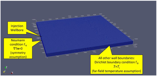
Figure 3. A mesh representing a 500 square-meter area of the Frio Formation. A Neumann boundary condition is imposed on the y-z plane at x = 0, such that the temperature gradient is 0 to implement a symmetry assumption on that wall. All other walls have a Dirichlet boundary condition of T = T_i imposed to implement a far-field constant reservoir temperature assumption. The simulated injection wellbore perforation interval was configured to −1527.5 m to −1533.75 m with respect to the z-axis at a y-axis location of 500 m. The injection fluid and reservoir initial temperature was configured to be T_i = 58.4 C. The injection mass flow rate was configured to be 3.0 kg/s.

The overburden saturated rock density was configured to ρ_S = 2260 kg/m³ [23]. The far field pressure on the boundary furthest from the injection perforation zone and above the shale (caprock) layer is given a Dirichlet boundary condition set equal to the initial reservoir pressure P_i = 148 bar. A homogeneous Neumann boundary condition ($\nabla P\cdot n=0$) is imposed for pressure along the plane of symmetry.

The reservoir water velocity is configured to be initially quiescent. At simulation time t_0, the injectant mass flow rate is defined to be 3 kg/s, which remains until t = 7 days have elapsed, after which the injectant mass flow rate is defined to be 0 kg/s to simulate pump shutoff. From t = 7 days to t = 30 days, the water–rock interaction in the reservoir chemically equilibrates.

Multiple grid configurations consisting of an initial control-volume count of 100 × 100 × 16, 100 × 100 × 32, 200 × 200 × 16, 40 × 40 × 16, 40 × 40 × 32, 40 × 40 × 64, 80 × 80 × 16, 20 × 20 × 08, 20 × 20 × 16, and 20 × 20 × 32 were used. Simulations were executed with deal.II adaptive mesh refinement (AMR) enabled.

2.11.2. Lithologic Configuration

The Frio Formation lithology was modeled as a five-layer shale-sandstone system according to the depths and layers given in Table 1. The initial time t = t₀ compositions of the shale and sandstone are given in Table 4 in terms of solid-phase volume fraction and grain radii. Minerals with an initial volume fraction of 0 are minerals not present at the start of the simulation but are allowed to form through precipitation according to the kinetic mechanism specified by Equations (50) through (55). Poroelastic rock properties defined in the simulation are given in Table 5. The initial and boundary concentrations of solutes residing in the pore space formation water are given in Table 6.

Table 4. The initial and boundary formation lithology and porosity.

Mineral	Volume Fraction	Grain Radius, mm
Shale
Calcite, CaCO3	0.20	0.001
Quartz, SiO2	0.28	0.02
Halite, NaCl	0.00	0.01
K-Feldspar, KAlSi3O8	0.01	0.03
Illite, (0.65 K, 0.08 Na) (2.27 Al, 0.14 Fe, 0.2 Mg)3.41 SiO10(OH)2	0.41	0.0001
Initial shale porosity φ = 10%
Sandstone
Calcite, CaCO3	0.00	0.001
Dolomite, CaMg(CO3)2	0.00	0.020
Quartz, SiO2	0.55	0.02
Halite, NaCl	0.00	0.01
K-Feldspar, KAlSi3O8	0.13	0.03
Initial sandstone porosity φ = 32%

Table 5. The poroelastic property definitions.

Property	Shale	Sandstone
Bulk modulus, GPa [24]	10.1	8.83
Shear modulus, GPa [24]	11.0	9.64
Biot Modulus, GPa	8.82	12.56
Biot–Willis coefficient, αBW	0.35	0.79
Poisson’s ratio [25]	0.43	0.32
Tensile Strength, Pa [26]	8.25 × 106	8.45 × 106

Table 6. The initial and boundary formation water composition.

Solute	Concentration, M
	Initial Formation Water
OH−	1.0 × 10−7
Ca2+	2.5 × 10−3
Al(OH)3,aq	1.7 × 10−5
K+	5.0 × 10−5
SiO2,aq	1.0 × 10−3
CO2,aq	2.0 × 10−3
Na+	4.0 × 10−1
Fe2+	1.0 × 10−4
Mg2+	1.0 × 10−5
Cl−	4.0 × 10−1

3. Results and Discussion

Figure 4 shows a contour plot of pH and [$\mathrm{H}\mathrm{C}{\mathrm{O}}_3^{-}$] on a slice along the perforation zone after 4 days of injection at a mass rate of 3 kg/s, with a background color mapped to temperature. The bicarbonate ion concentration front identifies the bulk effluent, indicated by thick purple to gold contour lines (a.k.a. “plasma colormap”). The initial reservoir water has a much lower bicarbonate concentration of 0.002 M. From the figure, one can see an acidic front develops ahead of the effluent indicated by black to white contour lines. A lower temperature fluid region develops in the lower pH (acidic) region, indicated by a darker blue background. In our simulation, we see the same pH drop before the arrival of a high concentration of bicarbonate ion 30 m from the injection zone.

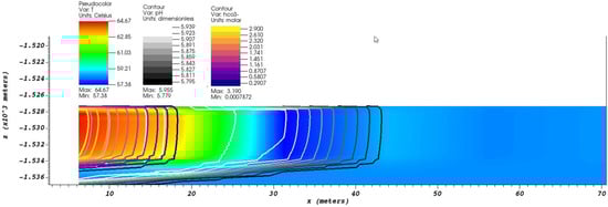
Figure 4. The contours of pH and [$\mathrm{H}\mathrm{C}{\mathrm{O}}_3^{-}$] on a slice along the perforation zone after 4 days of injection at a mass rate of 3 kg/s. The background is color-mapped to the formation water temperature.

Figure 5 shows snapshots of a simulation where an aqueous solution with CO_2,aq mass flow rate of 3 kg s⁻¹ is injected for 7 days into the lower sandstone. The upper row shows aqueous-phase temperature using a colormap in the range 58.4 °C (blue) to 60.0 °C (red) at selected times in units of days. The bottom row shows the source term volumetric energy generation rate S_T computed using Equation (23) divided by volumetric heat capacity ρc_p to give a temperature rate in units K s⁻¹. As expected, S_T vanishes (=0) after 7 days when injection terminates.

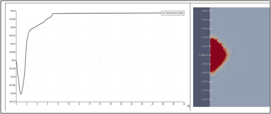
Figure 5. The simulated 30-day temperature profile at grid point (x = 30 m, y = 250 m, and z = −1530.625 m), corresponding to the location where the Frio Pilot observation well temperature sensor was placed. In the left plot, the y-axis is temperature in °C and the x-axis is time in days. The right image is a plot of temperature on the x-y plane at z = −1530.625 m. In the left plot, one can see the early arrival of a relatively lower temperature, low-pH diffusion front followed by a relatively higher temperature, high-alkalinity sweep front.

4. Conclusions

A short-term side-effect of subsurface CO₂ injection in brine-bearing sandstones is a developing low-pH front that forms ahead of the bulk water injectant, due to differences in solute diffusivity. The rapid dissolution of CaCO_3(s) and other carbonate minerals resulting from low-pH reservoir water can have significant environmental implications in geologic carbon sequestration. The dissolution of carbonate minerals can create unwanted pathways that will increase permeability and lead to a possible loss in CO₂ containment. Additionally, the formation of H₂CO₃ can be vulnerable to wellbore integrity through the corrosion of structures made from calcium-silica-hydrate compounds in Portland cements used to seal the annular volume between a casing and borehole wall. Temperature, pressure, and solute concentration measurements taken from an observation well during the Frio Pilot CO₂ sequestration experiment showed a reduction in aqueous-phase temperature with the arrival of the low-pH front, followed by a gradual rise in temperature upon the arrival of a high concentration of bicarbonate ion. We present a possible contributing factor to the variation in temperature between these two fronts by modeling aqueous-phase transient heat advection and diffusion, with the volumetric energy generation rate computed from solute-solvent interaction using the Helgeson–Kirkham–Flowers (HKF) model, which is based on the Born solvation model, for computing specific molar heat capacity and the enthalpy of charged electrolytes. We show how a simulated injectant water temperature profile is shown to agree with sampled temperature time-series data acquired from bottom hole observation well sensors. From Figure 4, we see our simulations reveal a lower temperature fluid region develop within an acidic region ahead of the bulk effluent. This acidic region is a diffusion front that is lower in temperature than the surrounding formation water being displaced and followed by a higher temperature sweep (effluent or injectant) front. The figure shows a plot of temperature vs. time at a single point on the slice, 30 m from the injection source, corresponding to the experimental observation well in the Frio experiment. From this plot, we see agreement between the simulated and experimental temperature profile.

The computation of aqueous-phase temperature during subsurface injection simulation is important for the accurate modeling of mineral kinetic mechanisms, as forward dissolution rates are governed by an Arrhenius model. In conclusion, the contribution of aqueous electrolytic reactions could play a role in the experimentally observed drop in temperature that corresponds to the arrival of a low-pH fluid region that forms ahead of the bulk effluent injectant, identified by a high concentration of bicarbonate ion ($\mathrm{H}\mathrm{C}{\mathrm{O}}_3^{-}$) that forms from dissociated aqueous CO₂.

References

- Hovorka, S.D.; Sakurai, S.; Kharaka, Y.K.; Nance, H.S.; Doughty, C.; Benson, S.M.; Freifeld, B.M.; Trautz, R.C.; Phelps, T.; Daley, T.M. Monitoring CO2 storage in brine formations: Lessons learned from the Frio field test one year post injection. In Proceedings of the 2006 UIC Conference of the Groundwater Protection Council, San Antonio, TX, USA, 23–25 January 2006; Gulf Coast Carbon Center: Washington, DC, USA, 2006. [Google Scholar]
- Kharaka, Y.K.; Cole, D.R.; Hovorka, S.D.; Gunter, W.D.; Knauss, K.G.; Freifeld, B.M. Gas-water-rock interactions in Frio Formation following CO2 injection: Implications for the storage of greenhouse gases in sedimentary basins. Geology 2006, 34, 577–580. [Google Scholar] [CrossRef]
- Pruess, K.; Müller, N. Formation dry-out from CO2 injection into saline aquifers: 1. Effects of solids precipitation and their mitigation. Water Resour. Res. 2009, 45, W03402. [Google Scholar] [CrossRef] [Green Version]
- Pruess, K. Formation dry-out from CO2 injection into saline aquifers: 2. Analytical model for salt precipitation. Water Resour. Res. 2009, 45, W03403. [Google Scholar] [CrossRef] [Green Version]
- Paolini, C.; Park, A.; Castillo, J. An investigation of the variation in the sweep and diffusion front displacement as a function of reservoir temperature and seepage velocity with implications in CO2 sequestration. In Proceedings of the 9th Annual International Energy Conversion Engineering Conference, San Diego, CA, USA, 31 July–3 August 2011; American Institute of Aeronautics and Astronautics: Reston, VA, USA, 2011. [Google Scholar]
- Park, A.J. Water-rock interaction and reactive-transport modeling using elemental mass-balance approach: I. The methodology. Am. J. Sci. 2014, 314, 785–804. [Google Scholar] [CrossRef]
- Boudreau, B.P. Diagenetic Models and Their Implementation: Modelling Transport and Reactions in Aquatic Sediments; Springer: Berlin/Heidelberg, Germany, 1997. [Google Scholar]
- Frio Brine Project Data, Frio Brine Pilot Study, Gulf Coast Carbon Center, Bureau of Economic Geology, Jackson School of Geosciences; The University of Texas at Austin, Regional Carbon Sequestration Partnership: Austin, TX, USA, 2018. Available online: https://edx.netl.doe.gov/dataset/frio-brine-project-data (accessed on 15 April 2022). [CrossRef]
- Carneiro, J.N.E.; Pasqualette, M.A.; Reyes, J.F.R.; Krogh, E.; Johansen, S.T.; Ciambelli, J.R.P.; Rodrigues, H.T.; Fonseca, R. Numerical Simulations of High CO2 Content Flows in Production Wells, Flowlines and Risers. In Proceedings of the OTC Brasil. Offshore Technology Conference, Rio de Janeiro, Brazil, 4–7 May 2015; p. 12. [Google Scholar]
- Helgeson, H.C.; Kirkham, D.H.; Flowers, G.C. Theoretical prediction of the thermodynamic behavior of aqueous electrolytes by high pressures and temperatures; IV, Calculation of activity coefficients, osmotic coefficients, and apparent molal and standard and relative partial molal properties to 600 degrees C and 5kb. Am. J. Sci. 1981, 281, 1249–1516. [Google Scholar]
- Bjerrum, N. Neuere Anschauungen über Elektrolyte. Ber. Der Dtsch. Chem. Ges. A B Ser. 1929, 62, 1091–1103. [Google Scholar] [CrossRef]
- Born, M. Volumen und Hydratationswärme der Ionen. Z. Für Phys. 1920, 1, 45–48. [Google Scholar] [CrossRef]
- Johnson, J.W.; Norton, D. Critical phenomena in hydrothermal systems: State, thermodynamic, electrostatic, and transport properties of H2O in the critical region. Am. J. Sci. 1991, 291, 541–648. [Google Scholar] [CrossRef]
- Anderson, G.M. Thermodynamics of Natural Systems, 2nd ed.; Cambridge University Press: Cambridge, UK, 2005. [Google Scholar]
- Griffiths, D.J. Introduction to Electrodynamics, 4th ed.; Cambridge University Press: Cambridge, UK, 2014. [Google Scholar]
- Marini, L. Geological Sequestration of Carbon Dioxide, Volume 11 Thermodynamics, Kinetics, and Reaction Path Modeling, 1st ed.; Elsevier Science: Amsterdam, The Netherlands, 2006. [Google Scholar]
- Tanger, J.C.; Helgeson, H.C. Calculation of the thermodynamic and transport properties of aqueous species at high pressures and temperatures; revised equations of state for the standard partial molal properties of ions and electrolytes. Am. J. Sci. 1988, 288, 19–98. [Google Scholar] [CrossRef]
- Shock, E.L.; Oelkers, E.H.; Johnson, J.W.; Sverjensky, D.A.; Helgeson, H.C. Calculation of the thermodynamic properties of aqueous species at high pressures and temperatures. Effective electrostatic radii, dissociation constants and standard partial molal properties to 1000 °C and 5 kbar. J. Chem. Soc. Faraday Trans. 1992, 88, 803–826. [Google Scholar] [CrossRef]
- Cherie. Thermodynamic Treatment of Ion-Solvent-Interactions: The Born Model. 2014. Available online: https://www.scribd.com/document/184980407/Born-Solvation-from-Cherie (accessed on 15 April 2022).
- Johnson, J.W.; Oelkers, E.H.; Helgeson, H.C. SUPCRT92: A software package for calculating the standard molal thermodynamic properties of minerals, gases, aqueous species, and reactions from 1 to 5000 bar and 0 to 1000 °C. Comput. Geosci. 1992, 18, 899–947. [Google Scholar] [CrossRef]
- Bangerth, W.; Hartmann, R.; Kanschat, G. deal. II—A general-purpose object-oriented finite element library. ACM Trans. Math. Softw. 2007, 33, 24. [Google Scholar] [CrossRef]
- Ganis, B.; Mear, M.E.; Sakhaee-Pour, A.; Wheeler, M.F.; Wick, T. Modeling fluid injection in fractures with a reservoir simulator coupled to a boundary element method. Comput. Geosci. 2014, 18, 613–624. [Google Scholar] [CrossRef]
- Huang, Z.Q.; Winterfeld, P.H.; Xiong, Y.; Wu, Y.S.; Yao, J. Parallel simulation of fully-coupled thermal-hydro-mechanical processes in CO2 leakage through fluid-driven fracture zones. Int. J. Greenh. Gas Control. 2015, 34, 39–51. [Google Scholar] [CrossRef]
- Gregory, A.R.; Kendall, K.K.; Lawal, A.S. Study Effects of Geopressured-Geothermal Subsurface Environment on Elastic Properties of Texas Gulf Coast Sandstones and Shales Using Well Logs, Core Data, and Velocity Surveys; Bureau of Economic Geology: Austin, TX, USA, 1980. [Google Scholar]
- Molina, O.; Vilarrasa, V.; Zeidouni, M. Geologic Carbon Storage for Shale Gas Recovery. Energy Procedia 2017, 114, 5748–5760. [Google Scholar] [CrossRef] [Green Version]
- Bruno, M.S.; Nakagawa, F.M. Pore pressure influence on tensile fracture propagation in sedimentary rock. Int. J. Rock Mech. Min. Sci. Geomech. Abstr. 1991, 28, 261–273. [Google Scholar] [CrossRef]
Publisher’s Note: MDPI stays neutral with regard to jurisdictional claims in published maps and institutional affiliations. |
© 2022 by the author. Licensee MDPI, Basel, Switzerland. This article is an open access article distributed under the terms and conditions of the Creative Commons Attribution (CC BY) license (https://creativecommons.org/licenses/by/4.0/).