Ultimate Pit-Limit Optimization Algorithm Enhancement Using Structured Query Language

Abstract

Three-dimensional block models are the most widely used tool for the study and evaluation of ore deposits, the calculation and design of economical pits, mine production planning, and physical and numerical simulations of ore deposits. The way these algorithms and computational techniques are programmed is usually through complex C++, C# or Python libraries. Database programming languages such as SQL (Structured Query Language) have traditionally been restricted to drillhole sample data operation. However, major advances in the management and processing of large databases have opened up the possibility of changing the way in which block model calculations are related to the database. Thanks to programming languages designed to manage databases, such as SQL, the traditional recursive traversal of database records is replaced by a system of database queries. In this way, with a simple SQL, numerous lines of code are eliminated from the different loops, thus achieving a greater calculation speed. In this paper, a floating cone optimization algorithm is adapted to SQL, describing how economical cones can be generated, related and calculated, all in a simple way and with few lines of code. Finally, to test this methodology, a case study is developed and shown.

1. Introduction

Most of the algorithms used in the study and evaluation of ore deposits [1,2,3], in the calculation and design of economical pits [4,5], in mine production planning [6] and in physical and numerical simulations of ore deposits [7,8,9,10] work with three-dimensional block models. A three-dimensional block model is a database in which each record represents a terrain block, i.e., a discrete rock element where the fields define its location (in an X, Y, Z coordinate system) and properties (density, lithology, ore grade, etc.). The information used to calculate the three-dimensional block model is obtained from the drillhole database. The different properties of the blocks can be estimated using various methods, such as nearest neighbor search, inverse distance weighting and geostatistical methods (simple kriging, ordinary kriging, cokriging or stochastic simulations).

In recent years, the computation of economical pits has undergone an important evolution to obtain better results and faster computational speeds. However, these improvements have traditionally been associated with the way in which the problem is attacked, either by means of the floating cone algorithm [11,12] and its corrections [13,14,15,16], the Korobov algorithm [17] and its corrected form [18], the Lerchs–Grossmann algorithm based on graph theory [19], pseudoflow [20], dynamic programming [21,22,23] or the genetic algorithm [24], rather than in the implementation of these techniques. It is important to note that the calculation times in economical pit design processes depend not only on the approach to the problem itself, but also on other factors regarding how the pit calculation method is implemented or the number of blocks that make up the block model.

The most commonly used programming languages for implementing three-dimensional block model computation techniques are usually through complex C++ [25], C# [26] or Python [27] libraries. It is important to note that commercial software works as a black box, preventing the user from knowing how the calculation methods are implemented. However, great advances in the management and processing of large databases have opened up the possibility of changing the way in which calculations with block models are related to the database. In 2013, the first open-pit optimization through a database was presented [28]. In that approach, an adaptation of the Lerchs–Grossmann algorithm was used.

Throughout this paper, we will show how to generate numerous open pits, relate them and calculate whether they are economical using structured query language (SQL). This new approach replaces the recursive path of traditional programming with a system of database queries. The aim is to reduce both the number of lines and the calculation time. To explain this methodology, the floating cone IV algorithm [16] will be used. It is a more complex floating cone algorithm and, as will be demonstrated, is able to take full advantage of the SQL JOIN clauses described below.

SQL is a domain-specific language designed to manage and retrieve information from relational database management systems. SQL is a declarative language, that is, you only have to tell the database system what you want to obtain, and the system will decide how to obtain it [29]. One of its main characteristics is the use of algebra and relational calculus to perform queries in order to retrieve, in a simple way, the information from the database, as well as to make changes in them. It is a database access language that exploits the flexibility and power of relational systems, thus allowing a wide variety of operations.

A relational database is a type of database that complies with the relational model [30], that is, it organizes data in one or more tables. Generally, each table represents an “entity type” (e.g., the block model or the set of economical cones that form the ultimate pit limit). The tables are composed of tuples (rows) that represent instances of that entity type (each of the blocks that make up the model). Each tuple (row) has a set of attributes for that instance (column names, also known as fields), for example, the lithology or ore grade of each block. Each tuple (row) is uniquely identified by an attribute called a primary key. Two tables can be related by a foreign key.

The main characteristic of the relational database is that it avoids the duplication of records, and at the same time, guarantees referential integrity; that is, if one of the records is deleted, the integrity of the remaining records will not be affected. In addition, thanks to the keys, the information can be easily accessed and retrieved at any time. SQL makes it possible to perform an endless number of queries to the database (join, delete, creation of new tables, calculation, etc.), which will be the basis on which the calculation method herein explained is founded.

Among all the relational database management systems (RDBMS) that use SQL to administer, define, manage and manipulate information (Oracle, Microsoft SQL Server, MySQL, SQLite), one of the most used and best cataloged today is PostgreSQL, as it is open source and has great stability, power, robustness, and ease of administration and implementation. Additionally, it uses a client/server system with threads for the correct processing of queries to the database [31,32].

2. Methodology for Applying SQL to a Three-Dimensional Block Model

The following section will describe the fundamental steps followed in implementing a floating cone algorithm using SQL. To be able to use the SQL database query language, and after much testing and improvement, the process has been divided into two parts:

• Gain an understanding of SQL in depth along with the different clauses that allow the generation of an open pit, relate them and calculate if they are economical. This point is dealt with in Section 2.1.
• Generate in PostgreSQL the tables to perform the necessary calculations and queries. This point is of great importance since the calculation times that are ultimately obtained will largely be dependent on it. This point is described in detail in Section 2.2.

Although this methodology is applied throughout this paper to a floating-cone-style algorithm, it could also be applied to many other algorithms whose objective is to search a database for records that meet certain conditions.

2.1. SQL JOINS

Before explaining the different tables generated to implement the floating cone algorithm, it is important to understand the SQL JOIN clause in detail. The SQL JOIN clause is one of the most powerful and interesting tools that SQL presents and is the fundamental basis on which the implementation explained throughout this paper is based. SQL JOIN clauses are used to combine rows from two or more tables based on a common field between them, thus returning data from different tables. For algorithms working with 3D block models, it is a quick way to relate blocks and cones (Figure 1). This point will be expanded as the implementation of the algorithm for the ultimate pit limit calculation is explained.

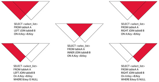
Figure 1. Graphical representation of how two cones that share blocks are related as a consequence of SQL JOIN clauses.

Although SQL JOIN clauses are divided into different types, they all work in a similar way. The SQL JOIN works with two selections, one of the selections called A or LEFT and the other B or RIGHT, which are joined with a logical condition. The ones that fulfill the union are common to both selections. On the other hand, there will be a part of selection A that does not fulfill the condition, and a part of selection B that does not fulfill it either. These three parts into which the union is divided can be selected in various ways using INNER, LEFT or RIGHT JOIN sentences, as can be seen in Figure 1 in which two cones (A and B) that share blocks are represented.

2.2. Generation of the Tables

When generating tables, it is important to consider that they can have tens of millions of tuples (rows), and a simple query to the database that relates several tables and has several selection conditions can take a long time to process, hence the importance of choosing a table structure that meets the following conditions:

• Tables with the minimum number of attributes are to be as simple and small as possible.
• Delete tuples from tables when they are no longer needed, thus also reducing the size of the tables.

The initial block model used for the calculation of economical pits will consist of a database managed by any database management system (DBMS). It will contain at least three attributes: a unique indicator or id for each block, and the weight and grade of the element to be evaluated. It is also necessary to know beforehand the size of the block in its three dimensions (sizeX, sizeY, sizeZ). From this initial database and with the different calculation parameters (recovery, sale price, slope angle, etc.), as well as considering the above conditions, three tables will be generated in PostgreSQL, which will be used in the calculation process: blks, blks2 and cones.

2.2.1. Blks Table

The blks table (Figure 2) will contain all the blocks to be entered into the calculation of the optimal pit. Table 1 shows in detail the different attributes that make up the blks table.

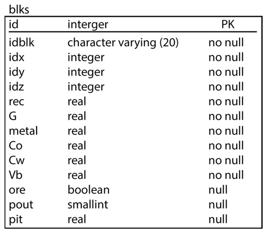
Figure 2. Table blks generated in PostgreSQL.

Table 1. Parameters and variables of the blks table depicted in Figure 2.

Symbol	Description
id	Unique identifier of each block that is generated incrementally when adding the blocks for calculation to the blks table. The blocks must be ordered from higher z to lower z, as we will use this id to order them and identify them in position. The lower id values correspond to those that are higher in z and the higher ones to those of a lower position
idblk	Id of the block of the original block model, to be used at the end of the calculation to put the results obtained in the original table
idx	Coordinates of the center of the block on the x-axis
idy	Coordinates of the center of the block on the y-axis
idz	Coordinates of the center of the block on the z-axis
rec	Percentage by weight of metal or ore recovered in the processing plant
G	Average concentration of the chemical element of interest in the reservoir in the block. Usually expressed as a percentage, or as grams per tonne (g/t) (equivalent to parts per million, ppm) or ounces per tonne (oz/t)
metal	The metal or chemical element content of interest in the block. Calculated by multiplying the weight of the block by the grade
Co	Mining cost of ore: drilling, blasting, loading and transportation, and grade control; this cost is usually given on a per tonne or per cubic meter basis. It tends to be slightly higher than waste rock due to grade control costs, and the height of the mining benches is generally smaller. The cost is generally calculated per tonne or per cubic meter
Cw	Mining cost of waste rock: drilling, blasting, loading, hauling and dumping of material at the waste dump; the cost is generally calculated per tonne or per cubic meter
Cp	Ore processing cost: crushing, milling, processing, handling of concentrates, and administrative costs and other costs. This cost is usually calculated per tonne of ore processed
Vb	Represents the value of each of the blocks. It is important to note that the value of each block should be calculated assuming that the block is uncovered; i.e., the cost required to access the block should not be considered in the total costs [33]. Equation (1) is used to perform the valuation for each block
ore	Indicates which blocks are considered to be minerals
pout	Field indicating whether a block is outside the calculation already or not; i.e., if that block is inside an economical cone, its initial value will be = 0 (it is not inside the economical pit) or = 1 (it is inside the economical pit)
pit	Value of the selling price calculated in the optimization process
T	Tonnes of the block
Ps	Final selling price of the metal or ore. It is equal to the market price minus the costs of transport, freight, fines, smelting and royalties

The value of the block Vb shown in Figure 2 and Table 1 is calculated via the following equation:

$$Vb=\left\{\begin{array}{cc}\hfill T·\left(G·rec·Ps-Co-Cp\right)\hfill & , if G\ge \frac{Co + Cp-Cw}{Ps·rec}\hfill \\ \hfill T·\left(-Cw\right)\hfill & , for the rest\hfill \end{array}\right.$$

(1)

2.2.2. Blks2 Table

The second table generated is called blks2 (Figure 3). Initially, it will have the same tuples as the blks table, but will only contain the attributes strictly necessary to calculate the economical cones, i.e., the attributes idx, idy, idz and the value of block Vb. This table is related to the blks table by the “id” field. From this table, any blocks that are in an economical cone will be removed during the process to leave only the records that follow in the SQL resolution.

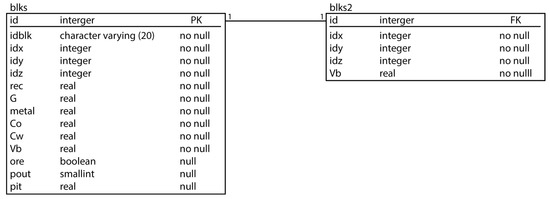
Figure 3. Table blks and blks2 and how they relate to each other.

To reduce the SQL response time, it is important to use the blks2 table instead of the source table blks, because, as mentioned before, this table, filled with only four selected attributes, will reduce in size as we delete the blocks that are already in an economical cone.

2.2.3. Cones Table

This last table (Figure 4) will contain the cones, both economical and non-economical, that are calculated per each and every block of ore, so the number of records in this table will be greatly increased. This is why the number of fields has to be reduced to the minimum possible so that the processing of the SQL is as fast as possible. Table 2 details each of the attributes that make up the cones table.

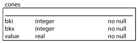
Figure 4. Cones table generated in PostgreSQL.

Table 2. Parameters and variables of the cones table depicted in Figure 4.

Symbol	Description
bki	Id of the ore block generating the cone
bkx	Id of each block that is in the cone generated by the block bki
value	Value of the bkx block

Therefore, if a new cone is formed by 100 blocks, 100 new records will be added to the cones table. For example, in the two-dimensional block model in Figure 5, the ore blocks would have an id 6 and id 7. The first cone generated would be in block id 6, and this cone would contain the blocks id 1, id 2, id 3 and id 6 itself. The next ore block would be id 7, and its cone would contain the blocks id 2, id 3, id 4 and id 7. Therefore, the cones table would consist of eight records (Table 3) in the case of the example in Figure 5.

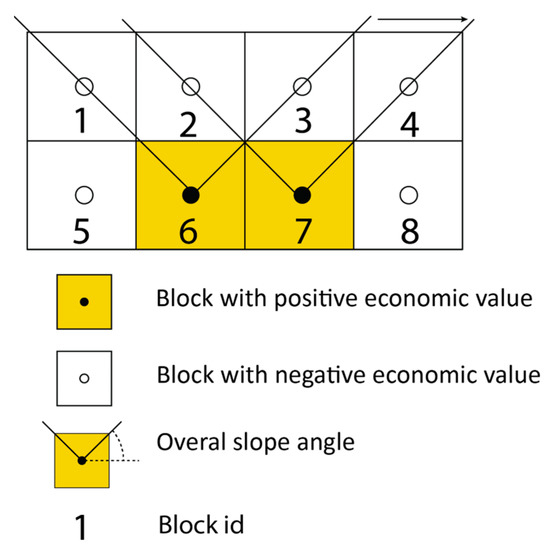
Figure 5. Two-dimensional block model.

Table 3. Example of the cones table with the two-dimensional block model in Figure 5.

bki	bkx	Value
6	1	Vb1
6	2	Vb2
6	3	Vb3
6	6	Vb6
7	2	Vb2
7	3	Vb3
7	4	Vb4
7	7	Vb7

Thus, a cone in the cones table is identified by the attribute bki, which is the identifier of the ore block that generates that cone. In this way, and with some simple SQL statements, you can select the cone generated by an ore block and query the value of that cone.

3. Implementation in PostgreSQL of the Floating Cone IV Algorithm

As mentioned above, the floating cone IV algorithm [16] will be used to explain this methodology. The floating cone IV algorithm is a more complex floating cone algorithm (Figure 6) and, as will be demonstrated, is able to take full advantage of the SQL JOIN clauses described above (Figure 1).

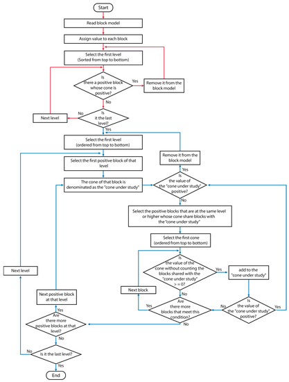
Figure 6. Flowchart of the floating cone IV algorithm [16]. The first part of the algorithm is represented by the red arrows. The second part of the algorithm is denoted by the blue arrows.

The floating cone IV algorithm (Figure 6) is characterized by presenting two main well-differentiated parts. In the first part of the algorithm (in Figure 6 represented with red arrows), those cones that are positive are removed from the block model, that is, it works like a regular floating cone algorithm. The implementation of the first part of the algorithm will be explained in Section 3.1. The second part of the algorithm (Figure 6, shown in blue arrows) searches for cones that, although individually not positive, comply in that the combination of two or more overlapping cones can generate positive values (Figure 7). The implementation of the first part of the algorithm is explained in Section 3.2.

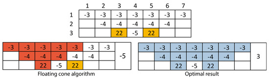
Figure 7. Example of a two-dimensional block model where two negative cones give a positive cone if studied together. While the classical floating cone algorithm does not find a positive result, the floating cone IV algorithm obtains a final cone with a positive value.

While it could be said that the floating cone method is outdated compared with the Lerschs–Grossmann or pseudoflow methods, this is not entirely correct, as the floating cone method has many advantages over these latter ones. Floating cone methods are widely regarded as robust algorithms that always provide a solution and are capable of being quickly verified in a simple way. Furthermore, floating cone methods can be easily programmed from scratch without the need to use external optimization libraries, as is often the case with other methods. It is important to note that, while the Lersch–Grossmann or pseudoflow methods provide a mathematically correct solution, sometimes it is not a viable solution from a mining operation point of view. On the other hand, although floating cone methods do not guarantee an optimal solution, they actually give one very close to it, with a difference within 2% [16]. Ramp and access design, or operational constraints, among many other factors, mean that the small differences obtained using the different methods of calculating economical open pits are not as important in the end. It is also important to note that the geological uncertainty far exceeds the differences obtained using the different methods, as the acceptable precision ranges of the geological modelization when estimating economical results vary between ±30% (conceptual study) and ±10% (feasibility study), according to [34].

In addition, floating cone methods have greater flexibility in designing algorithms to meet operational constraints (e.g., cones with minimum widths). For all these reasons, floating cone methods are a valid method for use in open-pit optimization.

3.1. First Part of the Algorithm

The algorithm searches for economical cones in descending order, i.e., starting from the top level (the level with the lowest Z value) to the last level of the block model (the level with the lowest Z value). As detailed above, the cones that are generated, whether economical or not, are initially stored in the cones table, for which the following SQL is executed (Algorithm 1 and Table 4):

Algorithm 1: PostgreSQL code of the first part of the floating cone IV
1:	“INSERT INTO cones (bki,bkx,value)
2:	(SELECT    B.id as bid, A.id as aid, A.Vb FROM
3:	(SELECT * FROM blks2 WHERE  idz ≥ Zs) A
4:	INNER JOIN (SELECT * FROM blks2 WHERE Vb > 0 AND idz = Zs) B
5:	ON(ATAN(SQRT(POWER(((A.idx-B.idx) * sicex),2) + POWER(((A.idy-B.idy) * sicey),2))/((A.idz-B.idz) * sicez + plusz)) * 180 / pi() < α))”

Table 4. Parameters and variables of the cones table depicted in Algorithm 1.

Symbol	Description
A.id	Id of block A, block that can be part of a cone
A.Vb	Value of block A, to be stored in the cones table as value
A.idx	Coordinates of the center of block A on the x-axis
A.idy	Coordinates of the center of block A on the y-axis
A.idz	Coordinates of the center of block A on the z-axis
B.id	Id of block B, ore block that generates a cone
B.idx	Coordinates of the center of block B on the x-axis
B.idy	Coordinates of the center of block B on the y-axis
B.idz	Coordinates of the center of block B on the z-axis
sizeX	Block sizes on the x-axis
sizeY	Block sizes on the y-axis
sizeZ	Block sizes on the z-axis
Zs	Level under study
plusz	Value that allows the cone to be moved downwards (Figure 8)
α	α = 90° − γ
γ	Overall slope angle

An important point when generating the floating cone is where the apex of the cone is located. This issue is rarely mentioned in the literature. For this implementation, the variable “plusz” has been created. This variable allows for the movement of the cone down a distance with respect to the center of the block to take into account that, if the center of the block is considered the cone apex, the whole ore block could not be mined; an option to do so would be to consider plusz = sizeZ/2 (Figure 8) as the new apex position.

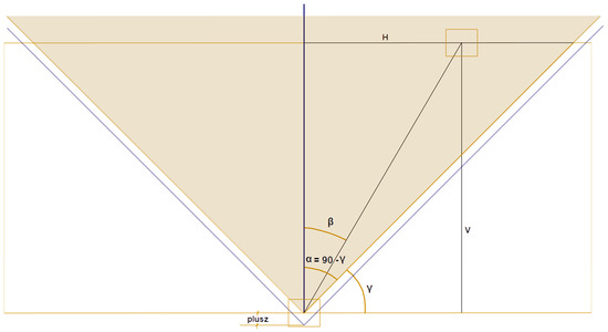
Figure 8. Two-dimensional graphical representation of the cone generation described in Algorithm 1. The parameters used for the calculation of the cone are explained in Table 4 and in Equations (2)–(4).

The first selection (referred to as LEFT or A) will select all blocks in the blks2 table (Figure 3) that are at the same level or higher than the level under study (Zs) (Figure 9A), for this purpose: A = (SELECT * FROM blks2 WHERE idz >= Zs), line 3 of Algorithm 1. The second selection (termed RIGHT or B) will select the ore blocks (Vb >0) from the blks2 table that are at the study level (Figure 9B), i.e., B = (SELECT * FROM blk2 WHERE Vb > 0 AND idz = Zs), line 4 of Algorithm 1.

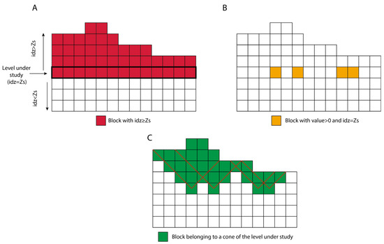
Figure 9. Two-dimensional block model: (A) graphical representation of the LEFT or A selection, selects all the blocks of the blks2 table that are at the same level or higher than the level under study (Zs); (B) graphical representation of the RIGHT or B selection, selects the mineral blocks (Vb > 0) of the blks2 table that are at the level Zs; (C) graphical representation of the final result of SQL.

The logical condition for the union of A and B is the selection of the blocks of A that belong to the cones of the blocks of B (Figure 9C). To determine the blocks that are located inside a cone, two angles are taken into account; on one hand, an angle complementary to the overall slope angle γ. This angle is called α. The second angle β is the angle shaped by the segment formed by joining the centers of the block that creates the cone (block B) and any block (block A) with respect to the z-axis, i.e., the vertical (Figure 8 and Figure 10). In such a way, those blocks of selection A that form an angle β ≤ α belong to the cone. The calculation of angle β can be expressed as follows:

$$\beta =atan\left(\frac{H}{V}\right)$$

(2)

where:

$$H=\sqrt[2]{{\left(\left(A.idx-B.idx\right)\ast sizex\right)}^2+{\left(\left(A.idy-B.idy\right)\ast sizey\right)}^2}$$

(3)

$$V=\left(A.idz-B.idz\right)\ast sizez+plusz$$

(4)

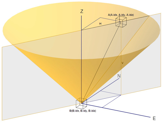
Figure 10. Three-dimensional graphical representation of the algorithm’s cone generation.

Equations (2)–(4) are defined graphically in Figure 8 and Figure 10. This equation is transformed into the code of line 5 of Algorithm 1, which expresses the logical condition of belonging to the cone and transforming the angle to degrees.

In this way, each mineral block of the selection RIGHT or B takes from the selection LEFT or A the blocks that are inside its cone. The id of B, the ore block that generates the cone, is stored in the cones table in the field bki, which is repeated in all the block records in that cone. The id and value of the blocks of the A selection are stored in the cones table in the fields bkx and Vb, respectively.

Once all the cones of a level have been added to the cones table, and before moving to the next level, the cones are evaluated for a positive value. Thanks to the bki field, the blocks that make up a cone can be quickly selected. Those blocks that are a part of an economical cone will be removed from the cones table and from the blks2 table and will be marked in the blks table with the value pout = 1. If any cone is detected at this stage as economical, the algorithm will start again at the first level looking for economical cones, since, as explained by the floating cone IV method, by removing blocks, some previously uneconomical cones may now be economical.

Once a level has been completed, the next level down is passed, repeating the process until the last level of the block model is reached. At this point, the first part of the floating cone IV algorithm is finished, i.e., all the blocks that are in any economical cone have been removed from the block model.

3.2. Second Part of the Algorithm

At this stage of the algorithm, only the cones with a negative value will remain in the cones table. The second part of the algorithm searches for combinations of two or more cones that share blocks and can generate a positive value. Following a strict descending order, the algorithm looks for, at the same level or higher, all the cones that share blocks with the “cone under study” and that fulfill the condition that the value of the cone, removing the blocks it shares with the “cone under study”, is ≥0 (as explained in Figure 1, this can be carried out with the LEFT JOIN statement where b.blks is null). Those cones that contribute with a positive value to the “cone under study” will be joined to it, and if the value of the “cone under study” becomes positive, it will be removed from the cones table and the process will be repeated again from the beginning. If the cone is still negative, the algorithm continues with the next cone until the end. When all the cones have been studied without removing any more cones from the set, the process is finished. All the blocks that have been removed from the block model will form the ultimate pit limit. The SQL syntax of this second part is presented in Algorithm 2 and Table 5.

Algorithm 2: PostgreSQL code of the second part of the floating cone IV
1:	“SELECT SUM (value) AS vvalue
2:	FROM (SELECT DISTINCT blx, valor FROM conos WHERE bki = i OR bki
3:	IN (SELECT conos.bki FROM conos WHERE bki ≤ idzmax and bki <> i) A
4	LEFT JOIN (SELECT * FROM conos WHERE bki = i) B
5:	ON conos.bkx = b.bkx WHERE b.bkx IS null
6:	GROUP BY cones.bki HAVING SUM (cones.value) ≥ 0)) c;”

Table 5. Parameters and variables of the cones table depicted in Algorithm 2.

Symbol	Description
vvale	Value of the cone
Bki = i	Block forming the “cone under study”
bkx	Id of each block that is in that economical cone
idzmax	Maximum id value of the level under study. Allows for the selection of the blocks that are at that level or higher in the SQL

Algorithm 2 is explained in Figure 11, where Figure 11A represents all cones remaining in the cones table above the idzmax level (the blocks colored with stripes belong to two cones at a time). The red-colored blocks build the “cone under study”. The mineral block forming the “cone under study” is defined as bki = i.

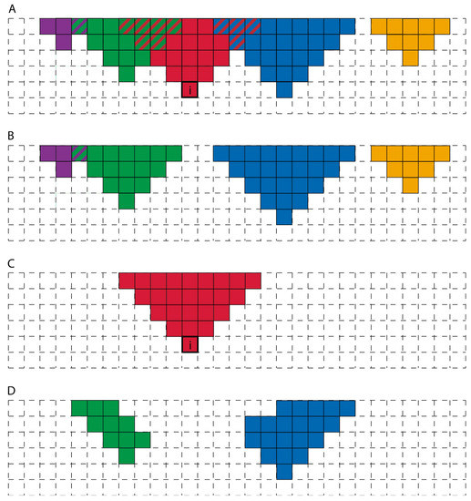
Figure 11. Two-dimensional block model where the steps of Algorithm 2 are graphically illustrated: (A) The colored blocks represent the cones remaining in the cones table above the idzmax level (the blocks colored with stripes belong to two cones at a time). The red-colored blocks form the “cone under study”. The mineral block forming the “cone under study” is defined as bki = i. (B) Colored blocks are selected by the LEFT selection clause of the LEFT JOIN clause, i.e., the cones above or at the same level of idzmax and with bki other than i. (C) RIGHT selection, cone formed by ore block i. (D) Blocks not in common with the “cone under study” but belonging to a cone sharing blocks with the cone under study. If either of these block groupings, green or blue, gives a positive value, it will join the “cone under study”.

The LEFT or A selection of the LEFT JOIN clause, A = (SELECT cones.bki FROM cones WHERE bki < idzmax AND bkx < > i), expressed in line 3 of Algorithm 2, selects all blocks in the cones table above idzmax without selecting the “cone under study” (Figure 11B). It selects only the bki field and not all fields in the cones table to perform the calculations as quickly as possible. The selection RIGHT or B selects the blocks that form the “cone under study”, i.e., the cone formed by the mineral block i (Figure 11C): B = (SELECT * FROM cones WHERE bki = i), expressed in line 4 of Algorithm 2.

Thanks to the join condition, LOGICAL_CODE = (cones.blks = b.blks) WHERE b.blks IS null, expressed in line 5 of Algorithm 2, only the blocks that are not in common with the “cone under study” and that are in a cone that does share blocks with the “cone under study” are selected (Figure 10D). That is, the “cone under study” (red color in Figure 11C) shares blocks with two cones (blue and green colors in Figure 11B); therefore, the result of the LEFT JOIN will be the blocks of the blue and green cones that are not shared with the red “cone under study” and that are presented in Figure 11D.

These blocks are grouped by the field bki, expressed in line 6 of Algorithm 2; that is, by the cone to which they belong, namely the blue ones on one side and the green ones on the other, and the condition is added that the sum of the values of the blocks of each group is: ≥0, GROUP BY cones.bki HAVING SUM(cones.value) ≥ 0. This way, the identifiers of the blocks that add value to the “cone under study” are obtained. In other words, if the sum of the values of the green blocks in Figure 11D is ≥0, they join the “cone under study”. It is the same with the blue blocks, if the sum is ≥0, they join the “cone under study”.

Finally, we have to evaluate if the “cone under study” with the new blocks added is positive. If it is positive, as in the first part of the algorithm, their blocks will be removed from the cones table and from the blks2 table and will be marked in the blks table with the value pout = 1. If it is negative, the algorithm continues with the next cone as the “cone under study”, as marked in the algorithm in Figure 6.

When the algorithm has run through all the cones from the top to the bottom without finding any cone junctions with a positive value, the process is finished. All the cones that were removed from the set, marked in the blks table as pout = 1, will be the ones that shape the ultimate pit.

4. Case Study

The deposit used to study the implementation described above is the Carles Au-Cu-Mo Skarn, located in the northwest of the Iberian Peninsula, approximately 45 km from Oviedo (Spain). The study area is located in the Río Narcea gold belt, one of the most important gold mining districts in the northwest of the Iberian Peninsula (Figure 12).

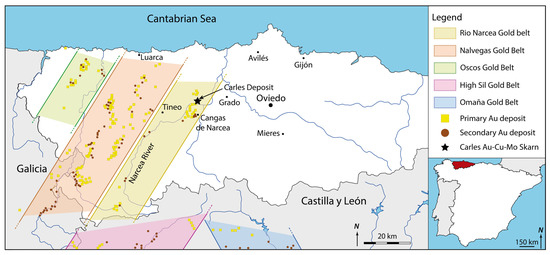
Figure 12. Geographical location of the Carles deposit.

The Carles deposit consists of a series of mineralizations associated with a granodiorite intrusion [35] that fits into the lithological contact of ferruginous sandstones and carbonate materials (Figure 13). The mineralizations are mainly developed as well-developed exoskarn exploiting tectonic and stratigraphic controls [36,37]; although endoskarn has been recorded, it is in the minority [38]. The maximum thickness of the mineralizations is approximately 50 m, but they can decrease sharply and even disappear completely, giving way to unmineralized marble (Figure 13) [38]. The main metallic minerals found in the deposit are magnetite, chalcopyrite, bornite, arsenopyrite, loellingite, pyrite, pyrrhotite and molybdenite. Gold is found as free gold and electrum, and occasionally as petzite and calaverite [37]. The Carles deposit (Carles N and Carles E, Figure 13) was exploited by Río Narcea Gold Mines S.A. by open-pit mining from 1998 to 2003, and from 2003 to 2006 by underground mining. Mining activity was resumed as underground mining in 2011, and continues to the present day by Orvana Minerals Corp.

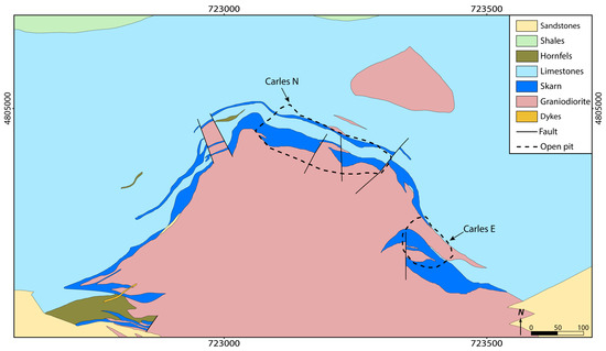
Figure 13. Geological map of the Carles deposit. Source: Río Narcea Gold Mines S.A.

For the case study, the Carles N orebody was modeled in three-dimensional form prior to mining (Figure 14). The orebody modeled is a quasi-tabular body with a southeast–northwest direction following the contact between the graniodiorite and the carbonate unit and dipping between 55° and 60° to the north. The orebody has a lateral continuity of approximately 425 m; vertically, it is much more irregular, with vertical continuity ranging from 370 m to 80 m. The body thickness decreases in depth from 25 to 30 m at surface height to 8 m in the lower levels. This modelization was developed from a database with a total of 87 drillholes (11,712.68 m). All drillhole information used in this study is available for free download at https://www.recmin.com/. Both the orebody modeling and the three-dimensional block model calculation were performed using freeware RecMin Free.

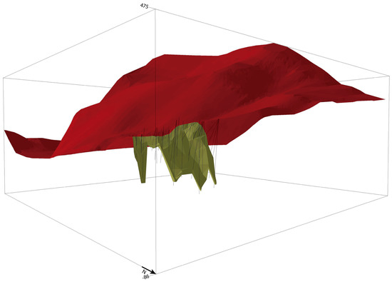
Figure 14. Three-dimensional model of the Carles N orebody before exploitation. The information on drillholes was provided by Río Narcea Gold Mines S.A.

The mining domain is discretized using (Figure 15) 10 × 10 × 10 m blocks, totaling 75,138 blocks. The interpolation method is anisotropic inverse distance weighting with a quadratic exponent (IDW2). When generating the three-dimensional block model, neither space nor geological constraints were considered in order to have a large block model for comparative testing. Similarly, in the case of the calculation of the ultimate pit limit, ideal conditions of Au price, costs and recoveries were considered; i.e., they were not the actual conditions and their only purpose was to obtain comparable results using both methods. The entire area used for the calculations is currently mined by both open-pit and underground mining. In other words, although this study was carried out using actual drillhole data, and the three-dimensional block model was calculated with the utmost rigor, it is only an academic exercise and should not be considered as a study for economical purposes.

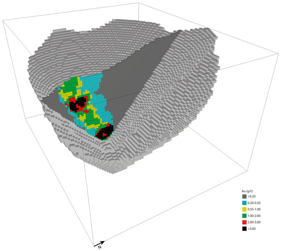
Figure 15. Three-dimensional representation of the ultimate pit calculated with RecMin Pro software. The parameters for the calculation of the ultimate pit limit are shown in Table 5. The size of the blocks is 10 × 10 × 10 m.

Two calculations were carried out for the comparison: the first calculation was performed using RecMin Free software using the floating cone algorithm programmed in VisualStudio.Net. The second calculation employed the floating cone IV method using. ProsgresSQL, as seen in this paper. The software utilized for the implementation and calculations was RecMin Pro, the evolution of RecMin Free currently under development. The same block model has been used for both calculations. The parameters used in the calculation of the economical open pit were as follows: 50° slope, mining cost USD 2/t, plant cost USD 10/t, recovery 95% and selling price USD 60/g, so the internal cut-off grade was 0.164 g/t and the cut-off breakeven was 0.211 g/t.

As can be seen in Table 6, the floating cone IV algorithm, when executed using SQL, shows a huge improvement from hours to minutes in computation time. For the calculations, we used an MSI computer with an i7 processor, 32 GB RAM, SSD solid disk, 4 GB graphics card and PostgreSQL 14 installed in local mode, which is a relatively common computer setup.

Table 6. Results obtained using the different methods.

Data	Floating Cone	Floating Cone IV (SQL)
Total no. of blocks	75,138	75,138
No. of pit blocks	36,782	37,078
Pit weight (t)	92,308,600.00	92,941,800.00
Ore weight (t)	33,336,000.00	33,519,000.00
Waste weight (t)	58,97,600.00	59,422,800.00
Ratio	1.769	1.773
Average ore grade (g/t)	0.983	0.981
Metal (g)	32,771,288.00	32,883,815.00
Calculation time	14 min 24 s	9 min 16 s

As can be seen in Table 6, the computation time obtained using the SQL method is significantly lower than that obtained with the classical programming method (approximately 35% lower). It is important to keep in mind that the floating cone IV algorithm is a much more complex algorithm than the traditional floating cone algorithm. As shown above, the floating cone IV algorithm comprises two major parts or loops. The first part is the classic floating cone algorithm, while the second part consists of a thorough search for negative-valued cones to obtain a positive-valued cone. That is, by using SQL, significantly more complex algorithms can be executed with better computation times.

5. Conclusions

Throughout this paper, we have shown how the floating cone optimization algorithm adapts to SQL. In this new methodology, the recursive path of traditional programming is replaced with a system of queries to the database using SQL. This novel approach in the industry allows numerous lines of code to be eliminated from the various loops, resulting in higher computational speed, as shown above in the case study.

The great advances in the management and processing of large databases have opened up not only the possibility of changing the method of relating calculations with block models to the database, but also the possibility of developing new work schemes, for example, implementing the methodology proposed in this paper in a client/server model. The client/server architecture would allow the calculations to be carried out on an external server; in this scheme, only the work orders would circulate through the network, but not the transit of data between tables. In this case, the capacity and speed of the server would be mainly responsible for the calculation speed.

SQL is often seen as an inflexible and unfriendly programming language and is quickly dismissed in favor of other programming languages. While this may seem true at first, after a thorough and detailed study of SQL, one can see that it is a very flexible and powerful tool. It is important to bear in mind that, although the SQL syntax is relatively similar among the main RDBMS, each one has characteristics that are important to consider in terms of optimizing the calculation times, especially in calculations that may contain tables with tens of millions of tuples (rows).

In conclusion, we have demonstrated how SQL works as a very powerful tool allowing the execution of complex algorithms that work with databases of three-dimensional block models obtaining great results. Although, in this paper, this methodology has been applied to a floating-cone-style algorithm, it can also be applied to many other algorithms whose objective is to search a database for records that meet certain conditions.

References

- Krzemień, A.; Fernández, P.R.; Sánchez, A.S.; Álvarez, I.D. Beyond the pan-european standard for reporting of exploration results, mineral resources and reserves. Resour. Policy 2016, 49, 81–91. [Google Scholar] [CrossRef]
- Rossi, M.E.; Deutsch, C.V. Mineral Resource Estimation; Springer Science & Business Media: Berlin/Heidelberg, Germany, 2013. [Google Scholar] [CrossRef]
- Glacken, I.M.; Snowden, D.V.; Edwards, A.C. Mineral resource estimation. In Mineral Resource and Ore Reserve Estimation—The AusIMM Guide to Good Practice; Edwards, A.C., Ed.; The Australasian Institute of Mining and Metallurgy: Melbourne, Australia, 2001; pp. 189–198. [Google Scholar]
- Hustrulid, W.; Kuchta, M. Open Pit Mine Planning and Design. Volume 1—Fundamentals. Taylor & Francis Group: Rotterdam, The Netherlands, 1995. [Google Scholar]
- Armstrong, D. Planning and design of surface mines–definition of mining parameters and ultimate pit definition. In Surface Mining, 2nd ed.; Kennedy, B.A., Ed.; Society for Mining, Metallurgy, and Exploration: Littleton, CO, USA, 1990; pp. 459–469. [Google Scholar]
- Osanloo, M.; Gholamnejad, J.; Karimi, B. Long-term open pit mine production planning: A review of models and algorithms. Int. J. Min. Reclam. Environ. 2008, 22, 3–35. [Google Scholar] [CrossRef]
- Liu, S.; Xiao, K.; Wang, X. Three-dimensional geological property model and its visualization. Geol. Bull. China 2010, 29, 1554–1557. [Google Scholar]
- Yao, L. Research on Three-Dimensional Property Modeling Method Based on Geostatistics; Peking University: Beijing, China, 2008. [Google Scholar]
- Bye, A. The strategic and tactical value of a 3D geotechnical model for mining optimization, Anglo Platinum, Sandsloot open pit. J. S. Afr. Inst. Min. Metall. 2006, 106, 97–104. [Google Scholar]
- Bowell, R.J.; Clarkson, B.; Prestia, A.; Thorne, S.; Donkervoort, L.; Smith, J.; Gear, J.; Pennington, J.; Griffiths, R.; Kiel, C.; et al. Sulfide Variation in the Coeur Rochester Silver Deposit: Use of Geologic Block Modeling in the Prediction and Management of Mine Waste. Econ. Geol. 2022, 118, 527–547. [Google Scholar] [CrossRef]
- Pana, M.T. The simulation approach to open pit design. In Proceedings of the 5th Symposium on the Application of Computers and Operations Research in the Mineral Industries (APCOM), Tucson, AZ, USA, 10–11 March 1965; pp. ZZ1–ZZ24. [Google Scholar]
- Carlson, T.R.; Erickson, J.D.; O’Brain, D.T.; Pana, M.T. Computer techniques in mine planning. Min. Eng. 1966, 18, 53–56. [Google Scholar]
- Wright, A. MOVING CONE II-A simple algorithm for optimum pit limits design. In Proceedings of the 28th Symposium on the Application of Computers and Operations Research in the Mineral Industries (APCOM), Golden, CO, USA, 20–22 October 1999; pp. 367–374. [Google Scholar]
- Khalou, K.R. Optimum Open Pit Design with Modified Moving Cone II Methods. J. Fac. Eng. 2007, 41, 297–307. [Google Scholar]
- Elahi, E.; Kakaie, R.; Yusefi, A. A new algorithm for optimum open pit design: Floating cone method III. J. Min. Environ. 2012, 2, 118–125. [Google Scholar] [CrossRef]
- Ares, G.; Castañón Fernández, C.; Álvarez, I.D.; Arias, D.; Díaz, A.B. Open Pit Optimization Using the Floating Cone Method: A New Algorithm. Minerals 2022, 12, 495. [Google Scholar] [CrossRef]
- David, M.; Dowd, P.A.; Korobov, S. Forecasting departure from planning in open pit design and grade control. In Proceedings of the 12th Symposium on the Application of Computers and Operations Research in the Mineral Industries (APCOM), Boulder, CO, USA, 7–11 April 1974; pp. F131–F142. [Google Scholar]
- Dowd, P.A.; Onur, A.H. Open-pit optimization. 1. Optimal open-pit design. Trans. Inst. Min. Metall. 1993, 102, A95–A104. [Google Scholar]
- Lerchs, H. Optimum design of open-pit mines. Trans CIM 1965, 68, 17–24. [Google Scholar]
- Bai, X.; Turczynski, G.; Baxter, N.; Place, D.; Sinclair-Ross, H. Pseudoflow method for pit optimization. In Whitepaper Geovia Whittle Dassault Systems; Dassault Systemes: Waltham, MA, USA, 2017. [Google Scholar]
- Koenigsberg, E. The optimum contours of an open pit mine: An application of dynamic programming. In Proceedings of the 17th Application of Computers and Operations Research in the Mineral Industry (APCOM), New York, NY, USA, 19–22 April 1982; pp. 274–287. [Google Scholar]
- Wilke, F.L. Determining the Optimal Untimate Pit Design for Hard Rock Open Pit Mines Using Dynamic Programming. Erzmetal 1984, 37, 139–144. [Google Scholar]
- Yamatomi, J.; Mogi, G.; Akaike, A.; Yamaguchi, U. Selective extraction dynamic cone algorithm for three-dimensional open pit designs. Proceedings of 25th Symposium on the Application of Computers and Operations Research in the Mineral Industries (APCOM), Brisbane, Australia, 9–14 July 1995; Australasian Institute of Mining and Metallurgy: Carlton, VIC, Australia, 1995; pp. 267–274. [Google Scholar]
- Denby, B.; Schofield, D. Open-pit design and scheduling by use of genetic algorithms. Trans. Inst. Min. Metall. 1994, 103, A21–A26. [Google Scholar]
- Deutsch, M.; Dağdelen, K.; Johnson, T. An Open-Source Program for Efficiently Computing Ultimate Pit Limits: MineFlow. Nat. Resour. Res. 2022, 31, 1175–1187. [Google Scholar] [CrossRef]
- Nikbin, V.; Ataee-Pour, M.; Shahriar, K.; Pourrahimian, Y. A 3D approximate hybrid algorithm for stope boundary optimization. Comput. Oper. Res. 2020, 115, 104475. [Google Scholar] [CrossRef]
- Yarmuch, J.L.; Brazil, M.; Rubinstein, H.; Thomas, D.A. Optimum ramp design in open pit mines. Comput. Oper. Res. 2020, 115, 104739. [Google Scholar] [CrossRef]
- Benito, R. Open pit limit optimization through databases: An open source for data analysis and reporting services. Min. Eng. 2013, 65, 11. [Google Scholar]
- Date, C.J. A Guide to the SQL Standard; Addison-Wesley Longman Publishing Co., Inc.: Boston, MA, USA, 1989. [Google Scholar]
- Codd, E.F. A relational model of data for large shared data banks. Commun. ACM 1970, 13, 377–387. [Google Scholar] [CrossRef]
- Ordóñez, M.P.Z.; Ríos, J.R.M.; Castillo, F.F.R. Administración de Bases de Datos con PostgreSQL; 3Ciencias: Alcoy, Spain, 2017; Volume 19. [Google Scholar] [CrossRef]
- Momjian, B. PostgreSQL: Introduction and Concepts; Addison-Wesley: New York, NY, USA, 2001; Volume 192. [Google Scholar]
- Lane, K.F. The Economic Definition of Ore: Cut-off Grades in Theory and Practice; Mining Journal Books Limited: London, UK, 1988. [Google Scholar]
- Lee, T.D. Planning and mine feasibility study—An owner perspective. In Proceedings of the 1984 NWMA Short Course “Mine Feasibility–Concept to Completion”, Northwest Mining Association, Spokane, WA, USA, 15–17 April 1984. [Google Scholar]
- Corretge, L.G.; Suarez, O.; Galan, G. Igneous Rocks. In Pre-Mesozoic Geology of Iberia; Dallmeyer, R.D., Garcia, E.M., Eds.; IGCP-Project 233; Springer: Berlin/Heidelberg, Germany, 1990; pp. 115–128. [Google Scholar] [CrossRef]
- Boixet, L. Morfología y Mineralogía del Skarn de Carlés, Asturias. Ph.D. Thesis, University of Oviedo, Oviedo, Spain, 1993; p. 84. [Google Scholar]
- Martín-Izard, A.; Boixet, L.; Maldonado, C. Geology and Mineralogy of the Carlés Gold-bearing Skarn. In Current Research Geology Applied to Ore Deposits; Fenoll Hach-Ali, P., Torres-Ruiz, J., Gervilla, F., Eds.; Univerisity of Granada: Granada, Spain, 1993; pp. 499–502. [Google Scholar]
- Martin-Izard, A.; Paniagua, A.; Garcıa-Iglesias, J.; Fuertes, M.; Boixet, L.; Maldonado, C.; Varela, A. The Carlés copper–gold–molybdenum skarn (Asturias, Spain): Geometry, mineral associations and metasomatic evolution. J. Geochem. Explor. 2000, 71, 153–175. [Google Scholar] [CrossRef]
Disclaimer/Publisher’s Note: The statements, opinions and data contained in all publications are solely those of the individual author(s) and contributor(s) and not of MDPI and/or the editor(s). MDPI and/or the editor(s) disclaim responsibility for any injury to people or property resulting from any ideas, methods, instructions or products referred to in the content. |
© 2023 by the authors. Licensee MDPI, Basel, Switzerland. This article is an open access article distributed under the terms and conditions of the Creative Commons Attribution (CC BY) license (https://creativecommons.org/licenses/by/4.0/).