Hierarchical Clustering Using One-Class Support Vector Machines

Abstract

This paper presents a novel hierarchical clustering method using support vector machines. A common approach for hierarchical clustering is to use distance for the task. However, different choices for computing inter-cluster distances often lead to fairly distinct clustering outcomes, causing interpretation difficulties in practice. In this paper, we propose to use a one-class support vector machine (OC-SVM) to directly find high-density regions of data. Our algorithm generates nested set estimates using the OC-SVM and exploits the hierarchical structure of the estimated sets. We demonstrate the proposed algorithm on synthetic datasets. The cluster hierarchy is visualized with dendrograms and spanning trees.

1. Introduction

The goal of cluster analysis is to assign data points into groups called clusters, so that the points in the same cluster are more closely related to each other than the points in different clusters [1]. In many applications, however, clusters often have subclusters, which, in turn, have sub-subclusters. Hierarchical clustering aims to find this hierarchical arrangement of the clusters. Requiring to specify neither the number of clusters nor the initial cluster assignment, hierarchical clustering is widely used for exploratory data analysis.

Typical procedures of the hierarchical clustering initially assign every data point to its own singleton cluster and successively merge the closest clusters until there is only one cluster left containing all of the data points [2]. In hierarchical clustering, cluster dissimilarities are commonly computed from the pairwise data point distances. However, the choices of computing inter-cluster distances can lead to fairly distinct cluster outcomes. For example, the result of linking the closest pair (single linkage) and the result of linking the furthest pair (complete linkage) are often different enough to cause difficulties in interpreting the cluster analysis in practice.

In this paper, we present a nonparametric hierarchical clustering algorithm based on the support vector method [3,4,5,6,7,8,9]. While typical hierarchical clustering algorithms use the pairwise data point distances, we propose to use a one-class support vector machine (OC-SVM) [10,11]. This is motivated by the recent work by Vert, R. and Vert, J [12] that the OC-SVM with the Gaussian kernel produces a consistent estimate of a density level set or a high-density region, where the free parameter λ affects the level of the estimated set.

Hence, we use the OC-SVM decision sets to directly estimate the high-density regions. In the data space, the OC-SVM decision boundary forms a set of contours enclosing the data points. We interpret the separated regions enclosed by the contours as clusters [13] and merge two clusters based on their connectivity in high-density regions. Since density level sets are hierarchical [14], we argue that a collection of the level sets from the OC-SVM naturally induces hierarchical clustering. Our algorithm finds the hierarchy of clusters from the family of OC-SVM level set estimates, which we obtain by varying the OC-SVM parameter λ in a continuum from zero to infinity.

Recently, de Morsier et al. [15] developed a hierarchical extension of support vector clustering. Rather than using the whole family of OC-SVM solutions, they select a level λ and consider the clusters in the corresponding OC-SVM solution. Then, they proceed to merge the clusters to find the cluster hierarchy. Two clusters are merged based on the average minimal distance between the cluster outliers. Thus, their cluster dissimilarities are also derived from the point distances, similarly to the conventional hierarchical clustering algorithms.

With the proposed hierarchical clustering method, we envision the following applications.

Anomaly detection: Anomaly detection is to identify deviations from the nominal data when combined observations of nominal and anomalous data are given. By detecting observations incoherent to existing clusters, one can develop early alarm systems of anomalous activities [16].

Image segmentation: Image segmentation is essential in computer vision for partitioning a digital image into a set of segments, such that pixels in the same segments are more similar to each other. A hierarchical structure found on the image segments can facilitate computer vision tasks [17,18].

We briefly review the OC-SVM in Section 2. Our hierarchical clustering algorithm based on the OC-SVM is presented in Section 3 and evaluated in Section 4. Conclusion remarks follow in Section 5.

2. One-Class Support Vector Machines

Suppose a random sample $\{{\mathbf{x}}_1,{\mathbf{x}}_2,\dots ,{\mathbf{x}}_n\}$, ${\mathbf{x}}_i\in {\text{ℝ}}^d$ is given. One-class support vector machines (OC-SVM) are proposed in [10,11] to estimate a set encompassing most of the data points in the space. The OC-SVM first maps each ${\mathbf{x}}_i$ to a high (possibly infinite) dimensional space $\mathscr{H}$ via a function $\Phi :{\text{ℝ}}^d\to \mathscr{H}$. A kernel function $k(\mathbf{x},{\mathbf{x}}^{\prime })=⟨\Phi \left(\mathbf{x}\right),\Phi \left({\mathbf{x}}^{\prime }\right)⟩$ corresponds to an inner product in $\mathscr{H}$. The OC-SVM finds a hyperplane in $\mathscr{H}$ that maximally separates the data points from the origin. The distance between the hyperplane and the origin is called the margin. To maximize the margin, the OC-SVM allows some data points inside the margin by introducing non-negative penalties ${\xi }_i$. More formally, the OC-SVM solves the following quadratic program:

$$\begin{array}{c}\underset{\mathbf{w},\mathbf{\xi }}{min}\frac{\lambda }{2}{\parallel \mathbf{w}\parallel }^2+\sum _{i=1}^n{\xi }_i\\ \text{subject}\text{to}⟨\mathbf{w},\Phi \left({\mathbf{x}}_i\right)⟩\ge 1-{\xi }_i,{\xi }_i\ge 0\text{for}i=1,2,\dots ,n\end{array}$$

where w ∈ $\mathscr{H}$ is the normal vector of the hyperplane and λ is the control parameter of the margin violations. In practice, the primal optimization problem is solved via its dual:

$$\begin{array}{c}\underset{\mathbf{\alpha }}{min}\frac{1}{2\lambda }\sum _{i,j}{\alpha }_i{\alpha }_j{K}_{ij}-\sum _i{\alpha }_i\\ \text{subject}\text{to}0\le {\alpha }_i\le 1\text{for}\forall i\end{array}$$

where $K_{ij}=k({\mathbf{x}}_i,{\mathbf{x}}_j)$ is the kernel matrix and ${\alpha }_i$ is a Lagrange multiplier associated with ${\mathbf{x}}_i$. Once the optimal solution is found, the decision function:

$$\begin{array}{c}\hfill f\left(\mathbf{x}\right)=⟨\mathbf{w},\Phi \left(\mathbf{x}\right)⟩=\frac{1}{\lambda }\sum _i{\alpha }_{i}k({\mathbf{x}}_i,\mathbf{x})\end{array}$$

(1)

defines the boundary $\{\mathbf{x}:f(\mathbf{x})=1\}$, which forms a set of contours enclosing the data points in ${\text{ℝ}}^d$. A more detailed discussion on the SVMs is available in [3].

3. Hierarchical Clustering Based on OC-SVM

In this section, we present our hierarchical clustering algorithm using a family of OC-SVM decision sets.

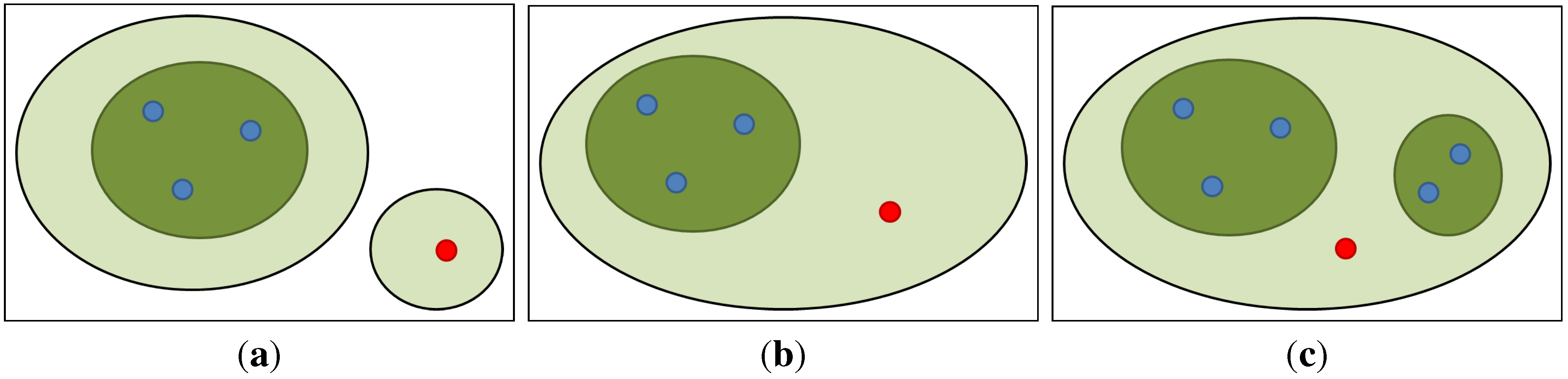
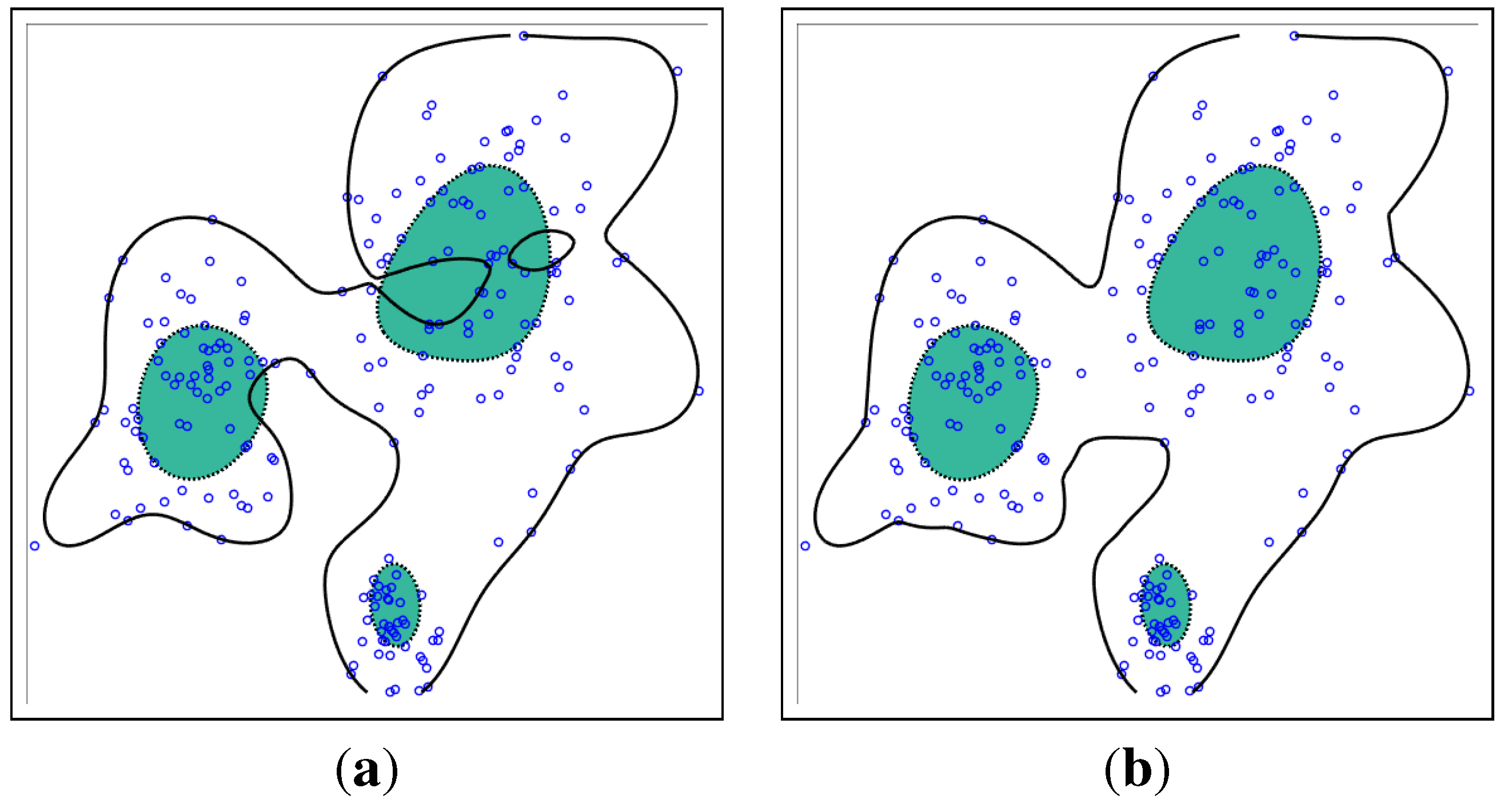
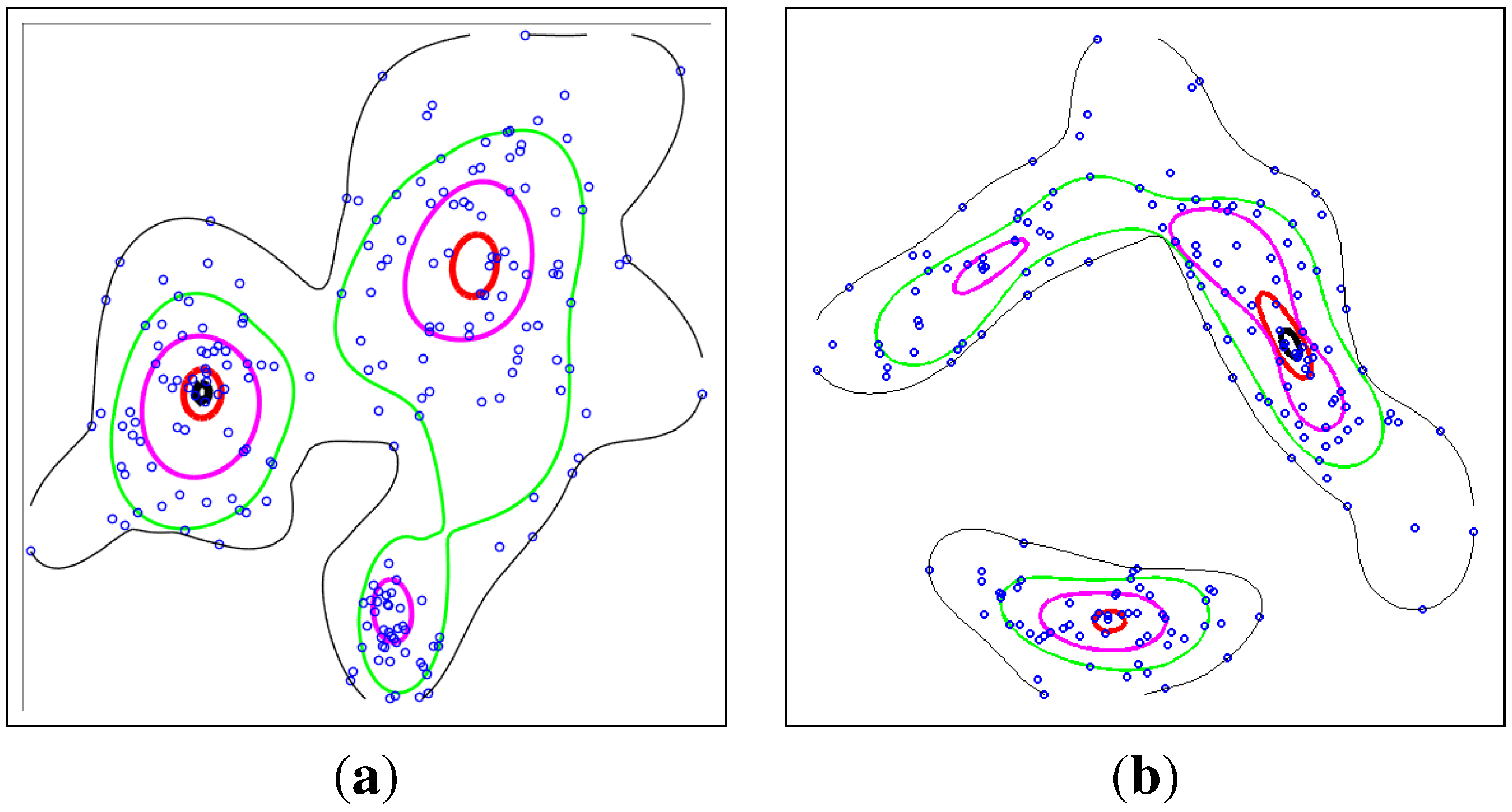
3.1. Nested OC-SVM Decision Sets

As discussed above, the OC-SVM decision set can be interpreted as a density level set estimator [12]:

$$\begin{array}{c}{\widehat{L^{\prime }}}_{\lambda }=\{\mathbf{x}:f_{\lambda }\left(\mathbf{x}\right)=\frac{1}{\lambda }\sum _i{\alpha }_i\left(\lambda \right)k({\mathbf{x}}_i,\mathbf{x})>1\}\end{array}$$

where λ is related to the level of the estimated set. Thus, we can generate a family of level set estimates by varying λ from infinity to zero. However, the set estimates are not necessarily nested, as illustrated in Section 4, while they should be. We enforce the decision sets to be nested by:

$$\begin{array}{c}{\widehat{L}}_{\lambda }=\bigcup _{\mu \ge \lambda }{\widehat{L^{\prime }}}_{\mu }.\end{array}$$

Then, these sets are clearly nested, so that an estimate at a higher value of λ is a subset of an estimate at a lower value of λ. We use these nested level set estimates ${\widehat{L}}_{\lambda }$ for hierarchical clustering.

We note that training the OC-SVM over the entire range of λ can be facilitated by the solution path algorithm by Lee and Scott [19]. The path algorithm finds the entire set of solutions as λ decreases from a large value toward zero. For sufficiently large λ, every data point falls between the hyperplane and the origin, so that $f\left(\mathbf{x}\right)<1$. As λ decreases, the margin width decreases, and data points cross the hyperplane ($f\left(\mathbf{x}\right)=1$) to move outside the margin ($f\left(\mathbf{x}\right)>1$). Throughout this process, ${\alpha }_i$ changes piecewise linearly in λ. We provide the derivation of the OC-SVM path algorithm in Appendix.

3.2. Hierarchical Clustering Using OC-SVM Decision Sets

Our approach is agglomerative and proceeds as λ decreases from infinity to zero. For sufficiently large λ, none of the data points are in the OC-SVM decision boundary. As λ decreases, data points cross the boundary and move into the decision set ${\widehat{L}}_{\lambda }$ until every data point is inside or on the boundary. A decision set may consist of one or more separated regions or clusters, and our algorithm finds the hierarchical arrangement of clusters during the process.

Algorithm 1 describes our hierarchical clustering approach. From the OC-SVM solution path algorithm, we obtain a set of breakpoints $({\lambda }_k,{\mathbf{\alpha }}^k)$. Each pair $({\lambda }_k,{\mathbf{\alpha }}^k)$ yields a decision set $L_{{\lambda }_k}$. The cluster collection $𝒟$ keeps track of the clusters in $L_{{\lambda }_k}$.

Algorithm 1 Hierarchical clustering based on one-class support vector machine (OC-SVM).

Input: $𝒯=\{{\mathbf{x}}_1,{\mathbf{x}}_2,\dots ,{\mathbf{x}}_n\}$

1: $\left\{({\lambda }_k,{\mathbf{\alpha }}^k)\right\}$← OC-SVM path algorithm $\left(𝒯\right)$ 2: $𝒟\leftarrow \left\{\right\}$ 3: for each k do 4:  $L_{{\lambda }_k}\leftarrow \{{\mathbf{x}}_j:f_{\mu }\left({\mathbf{x}}_j\right)>1,\mu \ge {\lambda }_k\}$ 5:  $L_{{\lambda }_k}^{new}\leftarrow L_{{\lambda }_k}-L_{{\lambda }_{k-1}}$ 6:  for each ${\mathbf{x}}_j\in L_{{\lambda }_k}^{new}$ do 7:   check connectivity from ${\mathbf{x}}_j$ to clusters in $𝒟$ 8:   if ${\mathbf{x}}_j$ is connected to none of the clusters in $𝒟$ then 9:    $𝒟\leftarrow 𝒟\cup \left\{{\mathbf{x}}_i\right\}$ 10:   else if ${\mathbf{x}}_j$ is connected to clusters in $𝒟$, say, $C_1,\dots ,C_m$ then 11:    merge $C_1,\dots ,C_m$ and $\left\{{\mathbf{x}}_j\right\}$ 12:   end if 13:  end for 14: end for

At step k, we first locate the data points newly included in the set $L_{{\lambda }_k}$ (Line 5). Each of these points is tested in Line 7 if it is connected to any clusters in $𝒟$. Our approach to test connectivity is geometric. A newly included data point ${\mathbf{x}}_j$ is determined to be connected to a cluster C if a path exists between ${\mathbf{x}}_j$ and any data point in C. If this is not the case, the path crosses the boundary and contains a segment of points y, such that $f\left(\mathbf{y}\right)<1$. To check the line segment, a number of sampled points can be used. We sample 20 points in our implementation.

Then, three cases arise from the connectivity test:

• if ${\mathbf{x}}_j$ is connected to none of the clusters, then the singleton cluster $\left\{{\mathbf{x}}_j\right\}$ is added to the cluster collection $𝒟$;
• if ${\mathbf{x}}_j$ is connected to exactly one cluster, then the singleton cluster $\left\{{\mathbf{x}}_j\right\}$ is merged into the cluster;
• if ${\mathbf{x}}_j$ is connected to more than one cluster, then all of these clusters and the singleton cluster $\left\{{\mathbf{x}}_j\right\}$ are merged.

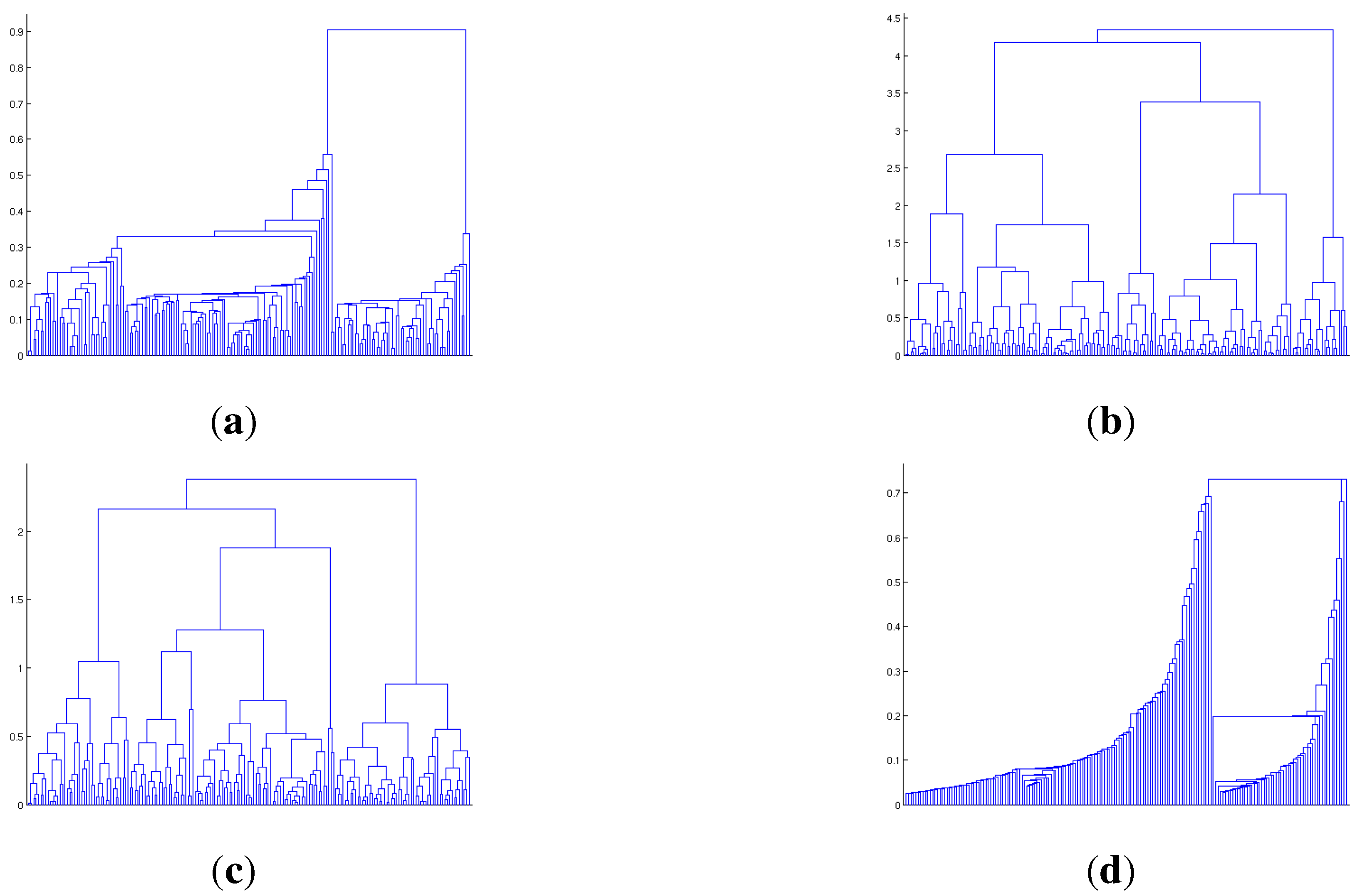
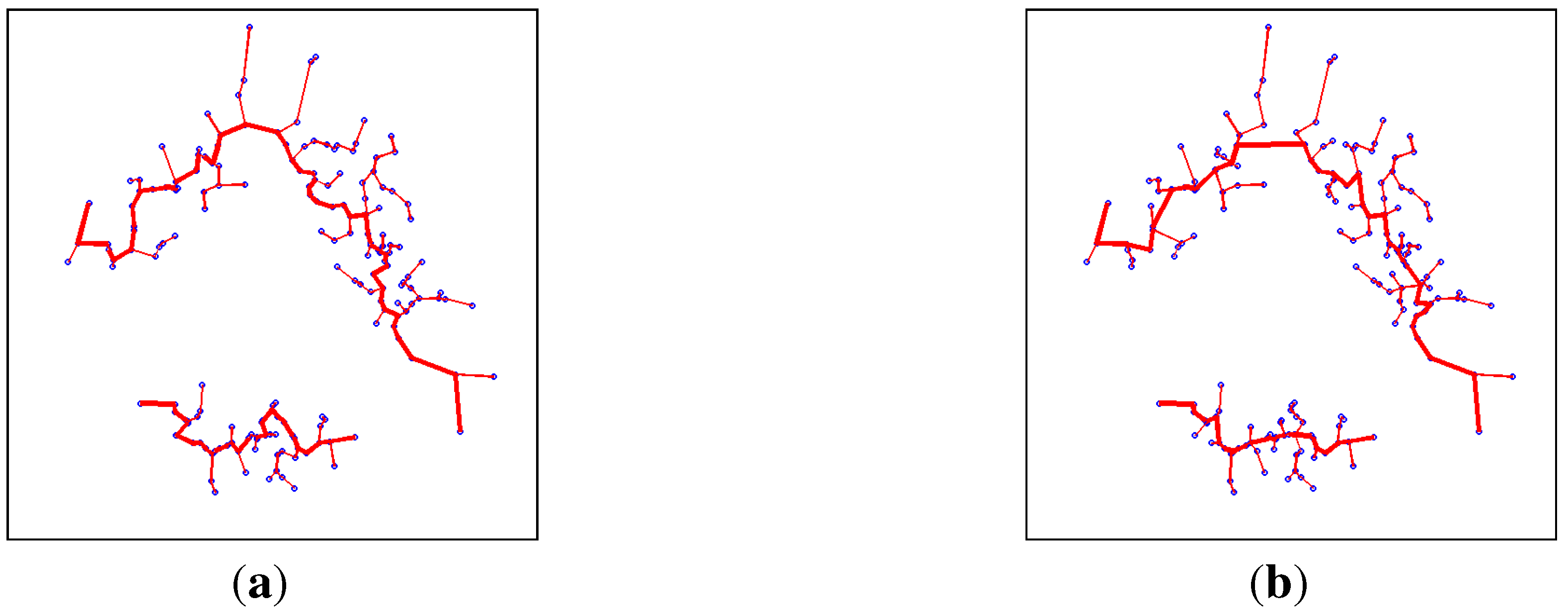
The cartoons in Figure 1 illustrate the three cases. Because of Case 3, a node in a dendrogram may have more than two child nodes. The merging process continues to the last breakpoint $({\lambda }_k,{\mathbf{\alpha }}^k)$. If $𝒟$ finishes with more than one cluster, then all of the remaining clusters are merged to form a single cluster containing all of the data points. Note that a spanning tree can also be derived from our algorithm by creating a tree edge connecting ${\mathbf{x}}_j$ with one of the cluster elements in Cases 2 and 3.

Figure 1. A new data point (red dot) is included in the decision set (solid contours). Based on the connectivity of the point to the existing (dark shaded) clusters, three cases arise: (a) the point is connected to none of the clusters, and a new cluster is formed; (b) the point is connected to exactly one cluster, and the cluster grows; or (c) the point is connected to more than one cluster, and the clusters are merged.

4. Experiments

We evaluate the proposed hierarchical clustering algorithm on two different datasets. The first dataset multi is from a three-component Gaussian mixture, and the second dataset banana is a benchmark dataset [20]. Our Matlab implementation of the OC-SVM path algorithm and the OC-SVM-based hierarchical clustering algorithm is available from the author’s website [21].

In our experiments, Gaussian kernel $k(\mathbf{x},{\mathbf{x}}^{\prime })=exp(-{\parallel \mathbf{x}-{\mathbf{x}}^{\prime }\parallel }^2/2{\sigma }^2)$ is used. Since this kernel maps all of the data points on a hypersphere in the same orthant, the OC-SVM principle, separating data points from the origin, is justified.

4.1. Gaussian Mixture Data

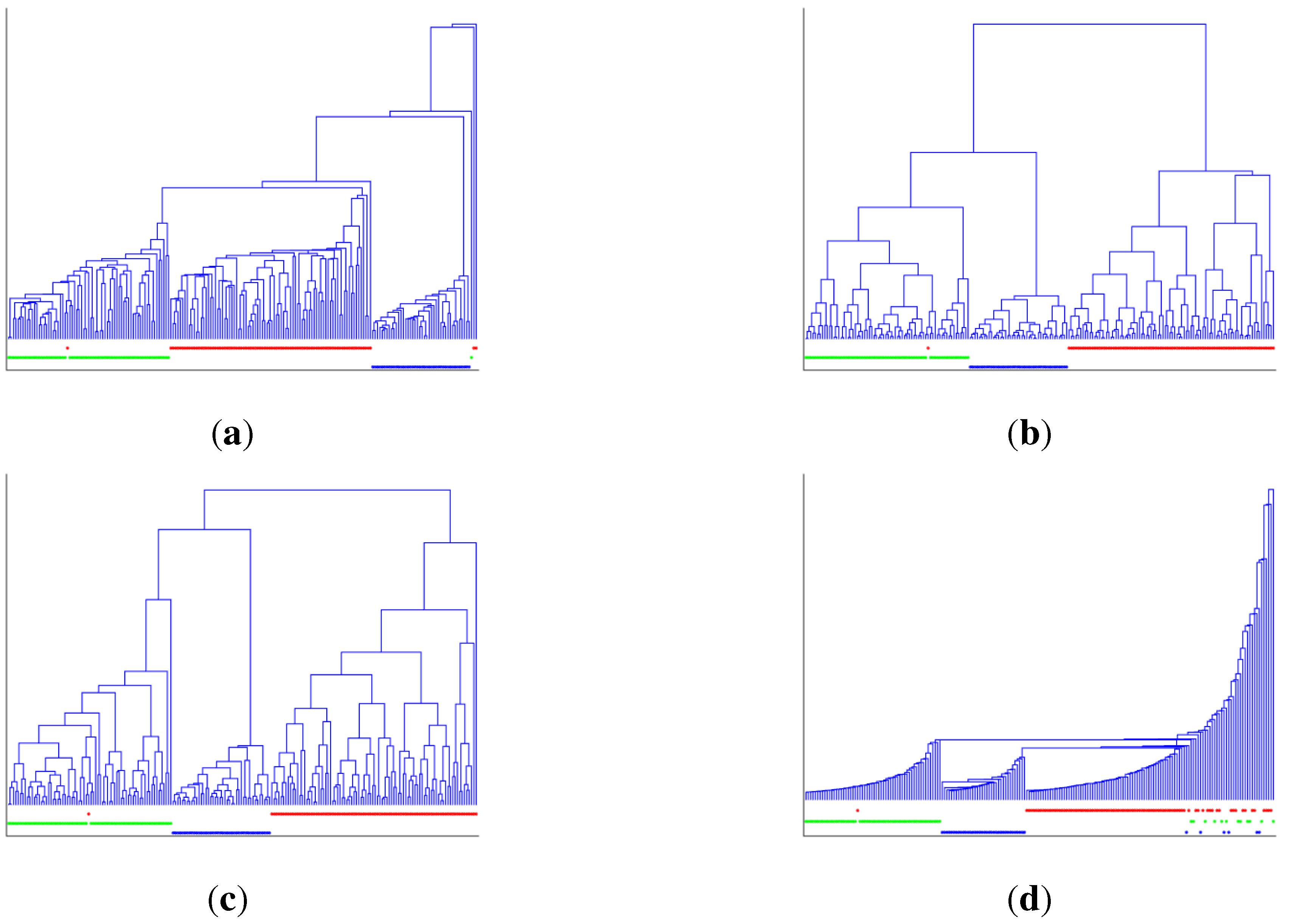
The multi is a set of 200 data points randomly drawn from a three-component Gaussian mixture distribution with uneven weights. Figure 2 shows the OC-SVM decision sets at two different values of λ. Each small circle represents a data point. As can be seen in Figure 2a, however, the decision set at the higher value of λ indicated by the shaded region is not completely contained inside the solid contour delineating the decision set at the lower value of λ. Thus, we modify the set estimates at a level λ to be the union of sets at higher levels, as explained in Section 3.1. Then, the boundaries do not cross each other, and the sets become properly nested (Figure 2b).

The five nested OC-SVM decision sets on multi data are illustrated in Figure 3a. The decision set at a certain level λ consists of one or more separated regions or contours. These contours are interpreted as cluster boundaries [13]. Then, the hierarchical structure of these clusters is clearly visible. The inner contours at higher levels are contained within the outer contours at lower levels. Thus, any pair of data points in the same cluster at a certain level remains together at lower levels. Note that the figure shows the three components of multi data.

Figure 2. The OC-SVM decision sets on multi data at $\lambda =22.60$ (shaded) and $1.26$ (contour). Small circles represent data points. (a) Two sets from the original OC-SVM are not nested. (b) With the modification in Section 3.1, the shaded region is completely contained inside the solid contour; thus, the sets are nested.

Figure 3. Nested OC-SVM decision boundaries at five different values of λ. Inner contours corresponds to higher values of λ and outer contours to lower values of λ. The sets are properly nested. (a) multi; (b) banana.

Our hierarchical clustering based on the OC-SVM is visualized with a dendrogram in Figure 4. Below each dendrogram, the ground truth cluster memberships are shown. The data points from the same Gaussian component are indicated by the dots of the same color and height. To compare with the conventional hierarchical clustering, the figure also displays the dendrograms from the single linkage, the complete linkage and the group average. While there are three true clusters in multi, it is not apparent in the classical agglomerative clustering results.

However, three components are clearly identifiable in Figure 4d obtained from the proposed OC-SVM hierarchical clustering. In the dendrogram, each of the three clusters grows until the larger one merges with the smaller one, and finally, all of the three clusters combine to form a single large cluster. Then, the cluster steadily grows until it encloses the rest of the outlying data points in the low-density regions. This observation is consistent with the nested decision boundaries in Figure 3.

Figure 4. Dendrograms from the classical hierarchical clustering of multi data: (a) single linkage, (b) complete linkage and (c) group average linkage. (d) Dendrogram from our hierarchical clustering algorithm based on the OC-SVM. Three clusters are clearly identifiable.

4.2. Benchmark Data

We repeat similar experiments on the banana benchmark data. The banana data were originally made for classification. In the experiments, only negative-class examples are used. As illustrated in Figure 3b, banana data have two distinct components: one is elongated banana-shaped, and the other is elliptical. The figure also displays the nested contours illustrating the nested OC-SVM decision sets.

The hierarchical clustering results are shown in Figure 5. Among the three classical agglomerative algorithms, only the single linkage seems to be able to identify the two data components. This result is expected, because the single linkage is advantageous to locate elongated clusters, while the complete linkage, which tends to produce compact spherical clusters, is disadvantageous. On the other hand, our method is more flexible and has successfully found the two data components, as can be seen Figure 5d. The valley in Figure 5d also indicates the possible subdivision of the banana-shaped cluster into two subclusters.

We further compare the single linkage and our approach using the spanning trees. Figure 6 shows the minimum spanning tree from the single linkage hierarchical clustering [22] and the spanning tree from the proposed OC-SVM hierarchical clustering. Both spanning trees look similar, but have differences. A major difference is in the longest paths in the data components. The thicker line segments in the figure indicate the longest paths. In the OC-SVM spanning tree, the nodes are located relatively in the “center”, and the path connecting the nodes shows the ridge of the data distribution.

Figure 5. Dendrograms from hierarchical clustering of banana data: (a) single linkage, (b) complete linkage, (c) group average linkage, and (d) OC-SVM. The two clusters are found from the single linkage and the OC-SVM hierarchical clustering.

Figure 6. (a) Minimum spanning tree on banana data from the single linkage, and (b) spanning tree from the OC-SVM hierarchical clustering. While both trees look similar, the longest path (thicker lines) in (b) tends to be in the middle of the data.

4.3. Computational Costs

The SVM solution path algorithm has $𝒪\left(n\right)$ breakpoints and complexity $𝒪(m^{2}n+n^{2}m)$, where m is the maximum number of points on the margin along the path [23]. At each breakpoint on the OC-SVM solution path, Algorithm 1 checks the connectivity of the newly included data points to the points in the existing clusters. If we assume that the newly included data points are on the margin, then the computational time of the proposed hierarchical clustering algorithm is $𝒪\left(n^{2}m\right)$. The computational costs on the multi and banana datasets are presented in Table 1.

Table 1. The computational costs for multi and banana datasets on an Intel i7-4790 3.60 GHz.

Computational Costs	multi	banana
# of breakpoints	504	404
OC-SVM path algorithm (sec)	0.19	0.15
Hierarchical clustering (OC-SVM) (sec)	1.04	1.17

Table 1. The computational costs for multi and banana datasets on an Intel i7-4790 3.60 GHz.

Computational Costs	multi	banana
# of breakpoints	504	404
OC-SVM path algorithm (sec)	0.19	0.15
Hierarchical clustering (OC-SVM) (sec)	1.04	1.17

5. Conclusions

In this paper, we have presented a hierarchical clustering algorithm employing the OC-SVM. Rather than using distance to indirectly find the high-density regions, we use the OC-SVM to estimate level sets and to directly locate the high-density regions. Our algorithm builds a family of nested OC-SVM decision sets over the entire range of control parameter λ. As each decision set induces a set of clusters, our algorithm finds the hierarchical structure of clusters from the family of decision sets. Dendrograms and spanning trees are used to visualize the results. Compared to the classical agglomerative methods, the proposed algorithm successfully identified the cluster components in the data sets. Future work may include comparing to other set estimators that yield nested decision sets as in [24] or kernel density estimation followed by thresholding.

References

- Duda, R.; Hart, P.; Stork, D. Pattern Classification, 2nd ed.; Wiley: New York, NY, USA, 2001. [Google Scholar]
- Hastie, T.; Tibshirani, R.; Friedman, J. The Elements of Statistical Learning; Data Mining, Inference and Prediction; Springer Verlag: New York, NY, USA, 2001. [Google Scholar]
- Schölkopf, B.; Smola, A. Learning with Kernels; MIT Press: Cambridge, MA, USA, 2002. [Google Scholar]
- Qi, Z.; Tian, Y.; Shi, Y. Successive overrelaxation for laplacian support vector machine. IEEE Trans. Neural Netw. Learn. Syst. 2015, 26, 667–684. [Google Scholar] [CrossRef] [PubMed]
- Qi, Z.; Tian, Y.; Shi, Y. Laplacian twin support vector machine for semi-supervised classification. Neural Netw. 2012, 35, 46–53. [Google Scholar] [CrossRef] [PubMed]
- Tian, Y.; Qi, Z.; Ju, X.; Shi, Y.; Liu, X. Nonparallel support vector machines for pattern classification. IEEE Trans. Cybern. 2014, 44, 1067–1079. [Google Scholar] [CrossRef] [PubMed]
- Qi, Z.; Tian, Y.; Shi, Y. Twin support vector machine with Universum data. Neural Netw. 2012, 36, 112–119. [Google Scholar] [CrossRef] [PubMed]
- Qi, Z.; Tian, Y.; Shi, Y. Structural twin support vector machine for classification. Knowl. Based Syst. 2013, 43, 74–81. [Google Scholar] [CrossRef]
- Qi, Z.; Tian, Y.; Shi, Y. Robust twin support vector machine for pattern classification. Pattern Recognit. 2013, 46, 305–316. [Google Scholar] [CrossRef]
- Tax, D.; Duin, R. Support vector domain description. Pattern Recognit. Lett. 1999, 20, 1191–1199. [Google Scholar] [CrossRef]
- Schölkopf, B.; Platt, J.; Shawe-Taylor, J.; Smola, A.; Williamson, R. Estimating the support of a high-dimensional distribution. Neural Comput. 2001, 13, 1443–1472. [Google Scholar] [CrossRef] [PubMed]
- Vert, R.; Vert, J. Consistency and convergence rates of one-class SVMs and related algorithms. J. Mach. Learn. Res. 2006, 7, 817–854. [Google Scholar]
- Ben-Hur, A.; Horn, D.; Siegelmann, H.; Vapnik, V. Support vector clustering. J. Mach. Learn. Res. 2001, 2, 125–137. [Google Scholar] [CrossRef]
- Hartigan, J. Clustering Algorithms; Wiley: New York, NY, USA, 1975. [Google Scholar]
- De Morsier, F.; Tuia, D.; Borgeaud, M.; Gass, V.; Thiran, J.P. Cluster validity measure and merging system for hierarchical clustering considering outliers. Pattern Recognit. 2015, 48, 1478–1489. [Google Scholar] [CrossRef]
- Yoon, S.H.; Min, J. An intelligent automatic early detection system of forest fire smoke signatures using gaussian mixture model. J. Inf. Process. Syst. 2013, 9, 621–632. [Google Scholar] [CrossRef]
- Manh, H.T.; Lee, G. Small object segmentation based on visual saliency in natural images. J. Inf. Process. Syst. 2013, 9, 592–601. [Google Scholar] [CrossRef]
- Yang, X.; Peng, G.; Cai, Z.; Zeng, K. Occluded and low resolution face detection with hierarchical deformable model. J. Converg. 2013, 4, 11–14. [Google Scholar]
- Lee, G.; Scott, C. The one class support vector machine solution path. In Proceedings of the IEEE International Conference on Acoustics, Speech and Signal Processing, Honolulu, HI, USA, 15–20 April 2007; Volume 2, pp. 521–524.
- Machine learning data set repository. Available online: http://mldata.org/repository/tags/data/IDA_Benchmark_Repository/ (accessed on 24 June 2015).
- OC-SVM HC. Available online: http://sites.google.com/site/gyeminlee/codes/ (accessed on 24 June 2015).
- Glower, J.; Ross, G. Minimum spanning trees and single linkage cluster analysis. Appl. Stat. 1969, 18, 54–64. [Google Scholar] [CrossRef]
- Hastie, T.; Rosset, S.; Tibshirani, R.; Zhu, J. The entire regularization path for the support vector machine. J. Mach. Learn. Res. 2004, 5, 1391–1415. [Google Scholar]
- Lee, G.; Scott, C. Nested support vector machines. IEEE Trans. Signal Process. 2010, 58, 1648–1660. [Google Scholar]
© 2015 by the authors; licensee MDPI, Basel, Switzerland. This article is an open access article distributed under the terms and conditions of the Creative Commons Attribution license (http://creativecommons.org/licenses/by/4.0/).