Article

Insights into the Time-Fractional Nonlinear KdV-Type Equations Under Non-Singular Kernel Operators


by
Mashael M. AlBaidani
* and
Rabab Alzahrani
Department of Mathematics, College of Science and Humanities, Prince Sattam Bin Abdulaziz University, Al Kharj 11942, Saudi Arabia
*
Author to whom correspondence should be addressed.
Symmetry 2026, 18(2), 391; https://doi.org/10.3390/sym18020391
Submission received: 20 January 2026 / Revised: 13 February 2026 / Accepted: 17 February 2026 / Published: 23 February 2026

Abstract

In this study, nonlinear fractional Korteweg–de Vries (KdV) type equations with nonlocal operators are studied using Mittag–Leffler kernels and exponential decay. The KdV equations are well known for its use in modeling ion-acoustic waves in plasma, oceanic dynamics, and shallow-water waves. As a result, mathematicians are working to examine modified and generalized versions of the basic KdV equation. In order to find the solutions of nonlinear fractional KdV equations, an extension of this concept is described in the current paper. The solution of fractional KdV equations is carried out using the well-known natural transform decomposition method (NTDM). To evaluate the problem, we employ the fractional operator in the Caputo–Fabrizio (CF) and the Atangana–Baleanu–Caputo sense (ABC) manner. Nonlinear terms can be handled with Adomian polynomials. The main advantage of this novel approach is that it might offer an approximate solution in the form of convergent series using easy calculations. The dynamical behavior of the resulting solutions have been demonstrated using graphs. Numerical data is represented visually in the tables. The solutions at various fractional orders are found and it is proved that they all tend to an integer-order solution. Additionally, we examine our findings with those of the iterative transform method (ITM) and the residual power series transform method (RPSTM). It is evident from the comparison that our approach offers better outcomes compared to other approaches. The results of the suggested method are very accurate and give helpful details on the real dynamics of each issue. The present technique can be expanded to address other significant fractional order problems due to its straightforward implementation.

1. Introduction

As old as classical calculus, fractional calculus literature dates back to 1695. The idea of the time-fractional derivative was initially brought up in a letter from L’Hospital to Leibnitz, and since then, development has been slow. Due to their extensive applications in the practical sciences, the integral and derivative of non-integer order are regarded as common topics of fractional calculus (FC). Due to its significance for modelling diverse processes in nature, this topic has become very popular among researchers. Systems controlled by memory, hereditary effects, and nonlocal interactions naturally give rise to fractional differential equations (FDEs), where the physical behavior is typically not adequately represented by classical integer-order models. The Riemann–Liouville (RL) fractional derivative, the Caputo fractional derivative [1], the Atangana–Baleanu–Caputo (ABC) fractional derivative [2], and the Caputo–Fabrizio fractional derivative [3] are among the several definitions of fractional calculus. Singular kernel and non-singular kernel types are the two broad categories into which fractional derivatives fall. Power-law memory is incorporated into singular kernel operators (like the RL and Caputo derivatives), but non-singular kernel operators (like the ABC and Caputo–Fabrizio derivatives) employ smooth kernels to prevent algebraic singularities [4]. An additional method for analyzing FC is provided by the CF and ABC derivative, which has uses in many different domains. Systems with memory and hereditary features can be modeled using it, and it offers the possibility of examining and characterizing intricate behaviors that integer-order derivatives are unable to adequately express. Their extensive use in modern research covers a variety of fields, including mathematical epidemiology [5,6], chaotic systems with singular and non-singular kernels [7], catalyzed hydrogenolysis of glycerol [8], oscillatory systems and electric networks [9], propagation of waves in complex media [10], nanofluid flow [11], bifurcation of neural network systems with delays [12], and nonlinear optical fibers [13].
The early theory and advancement of fractional derivatives and fractional differential equations (FDEs) have been rapidly noted throughout the past few decades. Authors like Kilbas et al. [14], Abbas et al. [15], Legnani et al. [16] and Hilfer [17] go into additional detail and grow on the area. Their study is primarily concerned with the theoretical issues related to FDEs and the systematic understanding of FC such as uniqueness and existence. Further concepts of FC can be found in the works by Hern’andez et al. [18], which cover the most recent advances in the theory of FDEs. FC’s applications in interdisciplinary disciplines like image processing and control theory were explored by Magin et al. [19] and Mainardi [20]. The modelling of numerous complicated natural and nonlinear processes benefits greatly from the use of fractional-order differential equations (FPDEs). A wide variety of processes and systems, memory, and other areas of mathematics have all benefited greatly from the work of FPDEs. Many natural occurrences can be accurately described by FPDEs because of their more convergent representation, whether it be in terms of time or space. FPDEs are of interest to scientists studying dielectric polarization, control theory, anomalous diffusion, and other issues relating to physical processes [21,22,23,24]. The largest contribution to explaining these kinds of systems is made by FPDEs because the non-integer order of the derivative describes hereditary features and situations where the future state is influenced by the previous state more precisely than integer order. As the integer order derivative is local and non-integer derivative is global, FPDEs have become more and more widespread. Some of the scientific issues and phenomena that FPDEs are used to represent include continuum mechanics, coloured noises, psychology, biology, acoustics, chemistry, and biology. Many areas of physics and hydrology, including [25,26,27,28,29] contain unique applications of FPDEs.
The construction of numerical and analytical approaches for the solution of FPDEs has become a major topic among scholars in recent years. Mathematicians never have it easy when trying to find numerical or analytical solutions to FPDEs. Fractional calculus has become a vibrant and influential field of study due to the necessity of resolving and exploring these complicated issues. Researchers have shown a great deal of interest in fractional PDEs in particular, which has led to the creation of numerous solutions. A number of efficient methods for examining both accurate and computational solutions to fractional differential equations have been developed in recent years. The following are some essential techniques such as the residual power series method [30], natural homotopy perturbation method [31], new iterative method [32], homotopy analysis method [33] the Legendre base method [34], the differential transform method [35], the Bernstein polynomial [36] and many more.
In particular, the KdV problem is well known as the ideal example of a perfectly solvable model, that is, a nonlinear partial differential equation whose solutions can be precisely and exactly described. Prototypical solitons are included in the solutions as well. The inverse scattering transform can be used to solve the KdV equation. The KdV equation’s basic mathematical theory is extensive, fascinating, and the focus of current mathematical research in general. The Korteweg–de Vries–Burgers equation is stated as [37]
D ζ μ ω ( ϑ , ζ ) + ω ϑ ϑ ϑ ( ϑ , ζ ) + ω ϑ ϑ ( ϑ , ζ ) + ω 2 ( ϑ , ζ ) ω ϑ ( ϑ , ζ ) = 0 , 0 < μ 1 ,
The modified KdV equation is [37]
ω ζ + ω 2 ( ϑ , ζ ) ω ϑ ( ϑ , ζ ) + ω ϑ ϑ ϑ ( ϑ , ζ ) = 0
and differs from the original KdV equation in the last nonlinear term only. The surface similarity is less important because of this, which results in some significant variances. On the other hand, the so-called “Miura transformation” connects these two equations at a deeper level. Understanding the function of nonlinear dispersion and the creation of structures like liquid drops leads to the modification of the KdV equation, which displays compactons, or solitons with compact support.
The modified Korteweg–de Vries (mKdV) equation is regarded as [38]
D ζ μ ω ( ϑ , ζ ) + 6 ω 2 ( ϑ , ζ ) ω ϑ ( ϑ , ζ ) + ω ϑ ϑ ϑ ( ϑ , ζ ) = 0 , 0 < μ 1 ,
The mKdV equation occurs in a wide range of disciplines, including biophysics, plasma science, shallow water models, and others. The mKdV equation’s dark multi-soliton solutions were obtained using a Darboux transformation [39]. Wazwaz [40] for obtaining the numerous solitary wave solutions of the mKdV equation using the extended tanh approach. Parkes [41] developed model solutions to the mKdV equation based on his observations on the tanh-coth expansion method. The authors of Ref. [42] developed an effective numerical method to investigate the asymptotic solution of Equation (3). With the use of phase portrait theory [43], the authors investigated compact solitary waves of the mKdV equation. The nonlocal symmetry, ideal systems, and explicit solutions of the mKdV equation were researched using the known Lax pair in [44].
We study the fractional mKdV equation utilising the CF and ABC operators as motivated by the previous literature. For the purpose of determining an approximation of the solution, we employ a hybrid strategy that elegantly combines the natural transform [45] and Adomian decomposition method [46]. By eliminating the necessity to calculate the fractional integrals or the fractional derivative in the recursive mechanism, the suggested approach streamlines the estimate of the series terms compared to the standard Adomian technique. NTDM avoids all round-off errors and doesn’t need discretization, linearization, perturbation, or specified assumptions. The suggested method offers reliable results that give precise solutions to the relevant problems. Our techniques generated infinite series in the numerical examples. After a specific number of iterations, it is found that the computational series approaches the precise outcome extremely closely, and the resulting series provides to us the results quite fast. In order to achieve accurate and approximate results quickly, this study offers a fundamental framework for researchers to analyze this method and use them in a range of applications. The fractional analysis carried out utilizing the suggested technique to look at the problems from a fractional perspective. To demonstrate a novel form of soliton solution that hasn’t been previously researched in the literature, we simulate the obtained solution for a few fractional orders. Recently, NTDM employed to solve time-fractional Fornberg–Whitham equation [47] and time-fractional coupled KdV equations [48]. The following is the paper’s outline: The key relationships are recalled in Section 2. We offer a general examination of the suggested technique in Section 3. The convergence analysis of the proposed method is covered in Section 4. The consideration equation’s solution is the focus of Section 5. We give the conclusions in Section 6.

2. Preliminaries

Here we we will discuss some basic definitions.
Definition 1. 
The fractional R-L integral is presented as [49]
I μ j ( φ ) = 1 Γ ( μ ) 0 φ ( φ ϖ ) μ 1 j ( ϖ ) d ϖ , μ > 0 , φ > 0 , a n d I 0 j ( φ ) = j ( φ ) .
Definition 2. 
The Caputo fractional derivative is presented as [49]
D φ μ j ( φ ) = I m μ D m j ( φ ) = 1 m μ φ 0 ( φ ϖ ) m μ 1 j m ( ϖ ) d ϖ ,
for m 1 < μ m , m N , φ > 0 , j C v m , v 1 .
Definition 3. 
The CF fractional derivative is presented as [49]
D φ μ j ( φ ) = 1 1 μ 0 φ exp μ ( φ ϖ ) 1 μ j ( ϖ ) d ϖ ,
having 0 < μ < 1 .
Definition 4. 
The fractional ABC derivative is presented as [49]
D φ μ j ( φ ) = B ( μ ) 1 μ 0 φ E μ μ ( φ ϖ ) μ 1 μ j ( ϖ ) d ϖ ,
with 0 < μ < 1 , and B ( μ ) represented the normalization function having B ( 0 ) = B ( 1 ) = 1 and E μ ( z ) = m = 0 z m Γ ( μ m + 1 ) is the Mittag–Leffler function.
Definition 5. 
The NT of ω ( ζ ) is presented as
N ( ω ( ζ ) ) = P ( λ , η ) = e λ ζ ω ( ζ ) d ζ , λ ( , ) .
For ζ ( 0 , ) , NT of ω ( ζ ) is presented as
N ( ω ( ζ ) H ( ζ ) ) = N ( ω ( ζ ) ) = P ( λ , η ) = e λ ζ ω ( ζ ) d ζ , λ ( 0 , ) ,
with H ( ζ ) illustrating the Heaviside function.
Definition 6. 
The function P ( λ , η ) inverse NT is presented as
N 1 [ P ( λ , η ) ] = ω ( ζ ) , ζ 0 .
Definition 7. 
The NT of D ζ μ ω ( ζ ) in Caputo sense is presented as [49]
N [ D ζ μ ω ( ζ ) ] = λ η μ N [ ω ( ζ ) ] 1 λ ω ( 0 ) .
Definition 8. 
The NT of D ζ μ ω ( ζ ) in CF sense is presented as [49]
N [ D ζ μ ω ( ζ ) ] = 1 1 μ + μ ( η λ ) N [ ω ( ζ ) ] 1 λ ω ( 0 ) .
Definition 9. 
The NT of D ζ μ ω ( ζ ) in ABC sense is presented as [49]
N [ D ζ μ ω ( ζ ) ] = B [ μ ] 1 μ + μ ( η λ ) μ N [ ω ( ζ ) ] 1 λ ω ( 0 ) .

3. Methodology

The procedure of NTDM for the below equation is discussed in this section.
D ζ μ ω ( ϑ , ζ ) = L ( ω ( ϑ , ζ ) ) + N ( ω ( ϑ , ζ ) ) + h ( ϑ , ζ ) ,
with initial source
ω ( ϑ , 0 ) = ϕ ( ϑ ) ,
with L , N , h ( ϑ , ζ ) indicating the linear, nonlinear and the source functions.

3.1. Case I ( N T D M C F )

On inserting NT to Equation (14) by means of Caputo–Fabrizio, we get
1 p ( μ , η , λ ) N [ ω ( ϑ , ζ ) ] ϕ ( ϑ ) λ = N [ M ( ϑ , ζ ) ] , N [ ω ( ϑ , ζ ) ] = ϕ ( ϑ ) λ + p ( μ , η , λ ) N [ M ( ϑ , ζ ) ] ,
with
p ( μ , η , λ ) = 1 μ + μ ( η λ ) ,
and
M ( ϑ , ζ ) = L ( ω ( ϑ , ζ ) ) + N ( ω ( ϑ , ζ ) ) + h ( ϑ , ζ ) .
On inserting inverse NT to Equation (16), we get
ω ( ϑ , ζ ) = N 1 ϕ ( ϑ ) λ + p ( μ , η , λ ) N [ M ( ϑ , ζ ) ] .
The nonlinear term N ( ω ( ϑ , ζ ) ) is represented as
N ( ω ( ϑ , ζ ) ) = i = 0 A i ,
Here A i represents the Adomian polynomials. The function ω ( ϑ , ζ ) series solution is presented as
ω ( ϑ , ζ ) = i = 0 ω i ( ϑ , ζ ) .
By using Equations (20) and (21) into (19), we get
i = 0 ω i ( ϑ , ζ ) = N 1 ϕ ( ϑ ) λ + p ( μ , η , λ ) N [ h ( ϑ , ζ ) ] + N 1 p ( μ , η , λ ) N i = 0 L ( ω i ( ϑ , ζ ) ) + A i .
By comparison of both sides, we have
ω 0 C F ( ϑ , ζ ) = N 1 ϕ ( ϑ ) λ + p ( μ , η , λ ) N [ h ( ϑ , ζ ) ] , ω 1 C F ( ϑ , ζ ) = N 1 p ( μ , η , λ ) N L ( ω 0 ( ϑ , ζ ) ) + A 0 , ω l + 1 C F ( ϑ , ζ ) = N 1 p ( μ , η , λ ) N L ( ω l ( ϑ , ζ ) ) + A l , l = 1 , 2 , 3 ,
Hence, the result of (14) in N T D M C F manner by using (23) into (21) as
ω C F ( ϑ , ζ ) = ω 0 C F ( ϑ , ζ ) + ω 1 C F ( ϑ , ζ ) + ω 2 C F ( ϑ , ζ ) +

3.2. Case II ( N T D M A B C )

On inserting NT to Equation (14) by means of Atangana–Baleanu–Caputo, we get
1 q ( μ , η , λ ) N [ ω ( ϑ , ζ ) ] ϕ ( ϑ ) λ = N [ M ( ϑ , ζ ) ] , N [ ω ( ϑ , ζ ) ] = ϕ ( ϑ ) λ + q ( μ , η , λ ) N [ M ( ϑ , ζ ) ] ,
with
q ( μ , η , λ ) = 1 μ + μ ( η λ ) μ B ( μ ) .
On inserting inverse NT to Equation (25), we get
ω ( ϑ , ζ ) = N 1 ϕ ( ϑ ) λ + q ( μ , η , λ ) N [ M ( ϑ , ζ ) ] .
The nonlinear term N ( ω ( ϑ , ζ ) ) is represented as
N ( ω ( ϑ , ζ ) ) = i = 0 A i .
The function ω ( ϑ , ζ ) series solution is presented as
ω ( ϑ , ζ ) = i = 0 ω i ( ϑ , ζ ) .
By using Equations (28) and (29) into (27), we get
i = 0 ω i ( ϑ , ζ ) = N 1 ϕ ( ϑ ) λ + q ( μ , η , λ ) N [ h ( ϑ , ζ ) ] + N 1 q ( μ , η , λ ) N i = 0 L ( ω i ( ϑ , ζ ) ) + A i .
By comparing both sides, we have
ω 0 A B C ( ϑ , ζ ) = N 1 ϕ ( ϑ ) λ + q ( μ , η , λ ) N [ h ( ϑ , ζ ) ] , ω 1 A B C ( ϑ , ζ ) = N 1 q ( μ , η , λ ) N L ( ω 0 ( ϑ , ζ ) ) + A 0 , ω l + 1 A B C ( ϑ , ζ ) = N 1 q ( μ , η , λ ) N L ( ω l ( ϑ , ζ ) ) + A l , l = 1 , 2 , 3 ,
Hence, the result of (14) in N T D M A B C manner by using (31) into (29) as
ω A B C ( ϑ , ζ ) = ω 0 A B C ( ϑ , ζ ) + ω 1 A B C ( ϑ , ζ ) + ω 2 A B C ( ϑ , ζ ) +

4. Convergence Analysis

The convergence for N T D M C F and N T D M A B C is stated as given.
Theorem 1. 
The N T D M C F result of (14) is unique if 0 < ( ϑ 1 + ϑ 2 ) ( 1 μ + μ ζ ) < 1 .
Proof. 
If G = ( C [ J ] , | | . | | ) is Banach space with J represents compact interval having norm | | ϕ ( ζ ) | | = m a x ζ J | ϕ ( ζ ) | ,∀ continuous function on J . Assume I : G G is a nonlinear mapping; thus,
ω l + 1 C = ω 0 C + N 1 [ p ( μ , η , λ ) N [ L ( ω l ( ϑ , ζ ) ) + N ( ω l ( ϑ , ζ ) ) ] ] , l 0 .
Let | L ( ω ) L ( ω * ) | < ϑ 1 | ω ω * | and | N ( ω ) N ( ω * ) |   < ϑ 2 | ω ω * | , where ω : = ω ( ϑ , ζ ) and ω * : = ω * ( ϑ , ζ ) are values of two separate functions and ϑ 1 , ϑ 2 are Lipschitz constants.
| | I ω I ω * | | m a x t J | N 1 [ p ( μ , η , λ ) N [ L ( ω ) L ( ω * ) ] + p ( μ , η , λ ) N [ N ( ω ) N ( ω * ) ] | ] m a x ζ J [ ϑ 1 N 1 [ p ( μ , η , λ ) N [ | ω ω * | ] ] + ϑ 2 N 1 [ p ( μ , η , λ ) N [ | ω ω * | ] ] ] m a x ζ J ( ϑ 1 + ϑ 2 ) N 1 [ p ( μ , η , λ ) N | ω ω * | ] ( ϑ 1 + ϑ 2 ) N 1 [ p ( μ , η , λ ) N | | ω ω * | | ] = ( ϑ 1 + ϑ 2 ) ( 1 μ + μ ζ ) | | ω ω * | |
I is contraction as 0 < ( ϑ 1 + ϑ 2 ) ( 1 μ + μ ζ ) < 1 . Thus the outcome of (14) is unique. □
Theorem 2. 
The N T D M A B C outcome of (14) is unique when 0 < ( ϑ 1 + ϑ 2 ) 1 μ + μ ζ μ Γ ( μ + 1 ) < 1 .
Proof. 
The proof of this theorem is same as of Theorem 1. □
Theorem 3. 
The N T D M C F result of (14) is convergent.
Proof. 
Let ω m = r = 0 m ω r ( φ , ζ ) . To show that ω m is a Cauchy sequence in G , assume
| | ω m ω n | | = m a x ζ J | r = n + 1 m ω r | , n = 1 , 2 , 3 , m a x ζ J N 1 p ( μ , η , λ ) N r = n + 1 m ( L ( ω r 1 ) + N ( ω r 1 ) ) = m a x ζ J N 1 p ( μ , η , λ ) N r = n + 1 m 1 ( L ( ω r ) + N ( ω r ) ) m a x ζ J | N 1 [ p ( μ , η , λ ) N [ ( L ( ω m 1 ) L ( ω n 1 ) + N ( ω m 1 ) N ( ω n 1 ) ) ] ] | ϑ 1 m a x ζ J | N 1 [ p ( μ , η , λ ) N [ ( L ( ω m 1 ) L ( ω n 1 ) ) ] ] | + ϑ 2 m a x ζ J | N 1 [ p ( μ , η , λ ) N [ ( N ( ω m 1 ) N ( ω n 1 ) ) ] ] | = ( ϑ 1 + ϑ 2 ) ( 1 μ + μ ζ ) | | ω m 1 ω n 1 | |
Let m = n + 1 , then
| | ω n + 1 ω n | | ϑ | | ω n ω n 1 | | ϑ 2 | | ω n 1 ω n 2 | | ϑ n | | ω 1 ω 0 | | ,
where ϑ = ( ϑ 1 + ϑ 2 ) ( 1 μ + μ ζ ) . So
| | ω m ω n | | | | ω n + 1 ω n | | + | | ω n + 2 ω n + 1 | | + + | | ω m ω m 1 | | , ( ϑ n + ϑ n + 1 + + ϑ m 1 ) | | ω 1 ω 0 | | ϑ n 1 ϑ m n 1 ϑ | | ω 1 | | ,
As 0 < ϑ < 1 , we get 1 ϑ m n < 1 . Therefore,
| | ω m ω n | | ϑ n 1 ϑ m a x ζ J | | ω 1 | | .
Since | | ω 1 | | < , | | ω m ω n | | 0 when n . Thus, the series ω m is convergent as ω m is a Cauchy sequence in G . □
Theorem 4. 
N T D M A B C solution of (14) is convergent.
Proof. 
The proof of this theorem is similar to that Theorem 3. □

5. Applications

We implemented NTDM to solve the nonlinear fractional KDV equations in this section.
Example 1. 
Assume fractional mKdV equation of the form [37]:
D ζ μ ω ( ϑ , ζ ) + 6 ω 2 ( ϑ , ζ ) ω ϑ ( ϑ , ζ ) + ω ϑ ϑ ϑ ( ϑ , ζ ) = 0 , 0 < μ 1 ,
with
ω ( ϑ , 0 ) = χ 4 χ 4 χ 2 ϑ 2 + 1 .
On inserting NT to Equation (38), we get
N [ D ζ μ ω ( ϑ , ζ ) ] = N { 6 ω 2 ( ϑ , ζ ) ω ϑ ( ϑ , ζ ) } N { ω ϑ ϑ ϑ ( ϑ , ζ ) } .
Now by using transform property
N [ ω ( ϑ , ζ ) ] = ω ( ϑ , 0 ) λ + N 6 ω 2 ( ϑ , ζ ) ω ϑ ( ϑ , ζ ) ω ϑ ϑ ϑ ( ϑ , ζ ) .
On inserting inverse inverse NT, we have
ω ( ϑ , ζ ) = χ 4 χ 2 4 χ 2 ϑ 2 + 1 N 1 η λ μ N 6 ω 2 ( ϑ , ζ ) ω ϑ ( ϑ , ζ ) + ω ϑ ϑ ϑ ( ϑ , ζ ) .
  • Implementation of N T D M C F
The series solution of ω ( ϑ , ζ ) is represented as
ω ( ϑ , ζ ) = l = 0 ω l ( ϑ , ζ ) .
The nonlinear term is indicated as ω 2 ω ϑ = l = 0 A l , So Equation (42) is taken as
l = 0 ω l + 1 ( ϑ , ζ ) = χ 4 χ 4 χ 2 ϑ 2 + 1 N 1 η ( λ μ ( λ η ) ) λ 2 N 6 l = 0 A l + ω ϑ ϑ ϑ ( ϑ , ζ ) .
Some Adomian polynomials are calculated as below:
A 0 = ω 0 2 ( ω 0 ) ζ , A 1 = ω 0 2 ( ω 1 ) ζ + 2 ω 0 ω 1 ( ω 0 ) ζ ,
By comparison of both sides of Equation (44), we get
ω 0 ( ϑ , ζ ) = χ 4 χ 4 χ 2 ϑ 2 + 1 ,
ω 1 ( ϑ , ζ ) = 192 χ 6 ϑ ( 16 ϑ 4 χ 4 32 ϑ 2 χ 3 + 40 ϑ 2 χ 2 + 16 χ 2 8 χ 7 ) ( 4 χ 2 ϑ 2 + 1 ) 4 μ ( ζ 1 ) + 1 ,
ω 2 ( ϑ , ζ ) = 1 ( 4 χ 2 ϑ 2 + 1 ) 7 ( 1152 χ 8 ( 3072 χ 10 ϑ 10 20480 χ 9 ϑ 8 + 23296 χ 8 ϑ 8 + 43008 χ 8 ϑ 6 114688 χ 7 ϑ 6 + 72576 χ 6 ϑ 6 36864 χ 7 ϑ 4 + 124416 χ 6 ϑ 4 + 5632 χ 5 ϑ 4 + 11264 χ 6 ϑ 2 93088 χ 4 ϑ 4 8192 χ 5 ϑ 2 23680 χ 4 ϑ 2 + 7680 χ 3 ϑ 2 256 χ 4 + 12924 χ 2 ϑ 2 + 256 χ 3 + 288 χ 2 144 χ 145 ) ) ( 1 μ ) 2 + 2 μ ( 1 μ ) ζ + μ 2 ζ 2 2 .
Lastly, the solution in N T D M C F manner is as follows:
ω ( ϑ , ζ ) = l = 0 ω l ( ϑ , ζ ) = ω 0 ( ϑ , ζ ) + ω 1 ( ϑ , ζ ) + ω 2 ( ϑ , ζ ) + , ω ( ϑ , ζ ) = χ 4 χ 4 χ 2 ϑ 2 + 1 192 χ 6 ϑ ( 16 ϑ 4 χ 4 32 ϑ 2 χ 3 + 40 ϑ 2 χ 2 + 16 χ 2 8 χ 7 ) ( 4 χ 2 ϑ 2 + 1 ) 4 μ ( ζ 1 ) + 1 1 ( 4 χ 2 ϑ 2 + 1 ) 7 ( 1152 χ 8 ( 3072 χ 10 ϑ 10 20480 χ 9 ϑ 8 + 23296 χ 8 ϑ 8 + 43008 χ 8 ϑ 6 114688 χ 7 ϑ 6 + 72576 χ 6 ϑ 6 36864 χ 7 ϑ 4 + 124416 χ 6 ϑ 4 + 5632 χ 5 ϑ 4 + 11264 χ 6 ϑ 2 93088 χ 4 ϑ 4 8192 χ 5 ϑ 2 23680 χ 4 ϑ 2 + 7680 χ 3 ϑ 2 256 χ 4 + 12924 χ 2 ϑ 2 + 256 χ 3 + 288 χ 2 144 χ 145 ) ) ( ( 1 μ ) 2 + 2 μ ( 1 μ ) ζ + μ 2 ζ 2 2 ) + .
  • Implementation of  N T D M A B C
The series solution of ω ( ϑ , ζ ) is represented as
ω ( ϑ , ζ ) = l = 0 ω l ( ϑ , ζ ) .
The nonlinear term is indicated as ω 2 ω ϑ = l = 0 A l , So Equation (42) is taken as
l = 0 ω l + 1 ( ϑ , ζ ) = χ 4 χ 4 χ 2 ϑ 2 + 1 N 1 η μ ( λ μ + μ ( η μ λ μ ) ) λ 2 μ N 6 l = 0 A l + ω ϑ ϑ ϑ ( ϑ , ζ ) .
The Adomian polynomials are calculated as stated in Equation (45). By comparing both sides of Equation (50), we obtain
ω 0 ( ϑ , ζ ) = χ 4 χ 4 χ 2 ϑ 2 + 1 ,
ω 1 ( ϑ , ζ ) = 192 χ 6 ϑ ( 16 ϑ 4 χ 4 32 ϑ 2 χ 3 + 40 ϑ 2 χ 2 + 16 χ 2 8 χ 7 ) ( 4 χ 2 ϑ 2 + 1 ) 4 1 μ + μ ζ μ Γ ( μ + 1 ) ,
ω 2 ( ϑ , ζ ) = 1 ( 4 χ 2 ϑ 2 + 1 ) 7 ( 1152 χ 8 ( 3072 χ 10 ϑ 10 20480 χ 9 ϑ 8 + 23296 χ 8 ϑ 8 + 43008 χ 8 ϑ 6 114688 χ 7 ϑ 6 + 72576 χ 6 ϑ 6 36864 χ 7 ϑ 4 + 124416 χ 6 ϑ 4 + 5632 χ 5 ϑ 4 + 11264 χ 6 ϑ 2 93088 χ 4 ϑ 4 8192 χ 5 ϑ 2 23680 χ 4 ϑ 2 + 7680 χ 3 ϑ 2 256 χ 4 + 12924 χ 2 ϑ 2 + 256 χ 3 + 288 χ 2 144 χ 145 ) ) [ μ 2 ζ 2 μ Γ ( 2 μ + 1 ) + 2 μ ( 1 μ ) ζ μ Γ ( μ + 1 ) + ( 1 μ ) 2 ] .
Lastly, the solution in N T D M A B C manner is as follows:
ω ( ϑ , ζ ) = l = 0 ω l ( ϑ , ζ ) = ω 0 ( ϑ , ζ ) + ω 1 ( ϑ , ζ ) + ω 2 ( ϑ , ζ ) + , ω ( ϑ , ζ ) = χ 4 χ 4 χ 2 ϑ 2 + 1 192 χ 6 ϑ ( 16 ϑ 4 χ 4 32 ϑ 2 χ 3 + 40 ϑ 2 χ 2 + 16 χ 2 8 χ 7 ) ( 4 χ 2 ϑ 2 + 1 ) 4 1 μ + μ ζ μ Γ ( μ + 1 ) 1 ( 4 χ 2 ϑ 2 + 1 ) 7 ( 1152 χ 8 ( 3072 χ 10 ϑ 10 20480 χ 9 ϑ 8 + 23296 χ 8 ϑ 8 + 43008 χ 8 ϑ 6 114688 χ 7 ϑ 6 + 72576 χ 6 ϑ 6 36864 χ 7 ϑ 4 + 124416 χ 6 ϑ 4 + 5632 χ 5 ϑ 4 + 11264 χ 6 ϑ 2 93088 χ 4 ϑ 4 8192 χ 5 ϑ 2 23680 χ 4 ϑ 2 + 7680 χ 3 ϑ 2 256 χ 4 + 12924 χ 2 ϑ 2 + 256 χ 3 + 288 χ 2 144 χ 145 ) ) [ μ 2 ζ 2 μ Γ ( 2 μ + 1 ) + 2 μ ( 1 μ ) ζ μ Γ ( μ + 1 ) + ( 1 μ ) 2 ] + .
By taking μ = 1 , we get the exact solution as
ω ( ϑ , ζ ) = χ 4 χ 4 χ 2 ( ϑ 2 6 χ 2 ζ ) 2 + 1 .
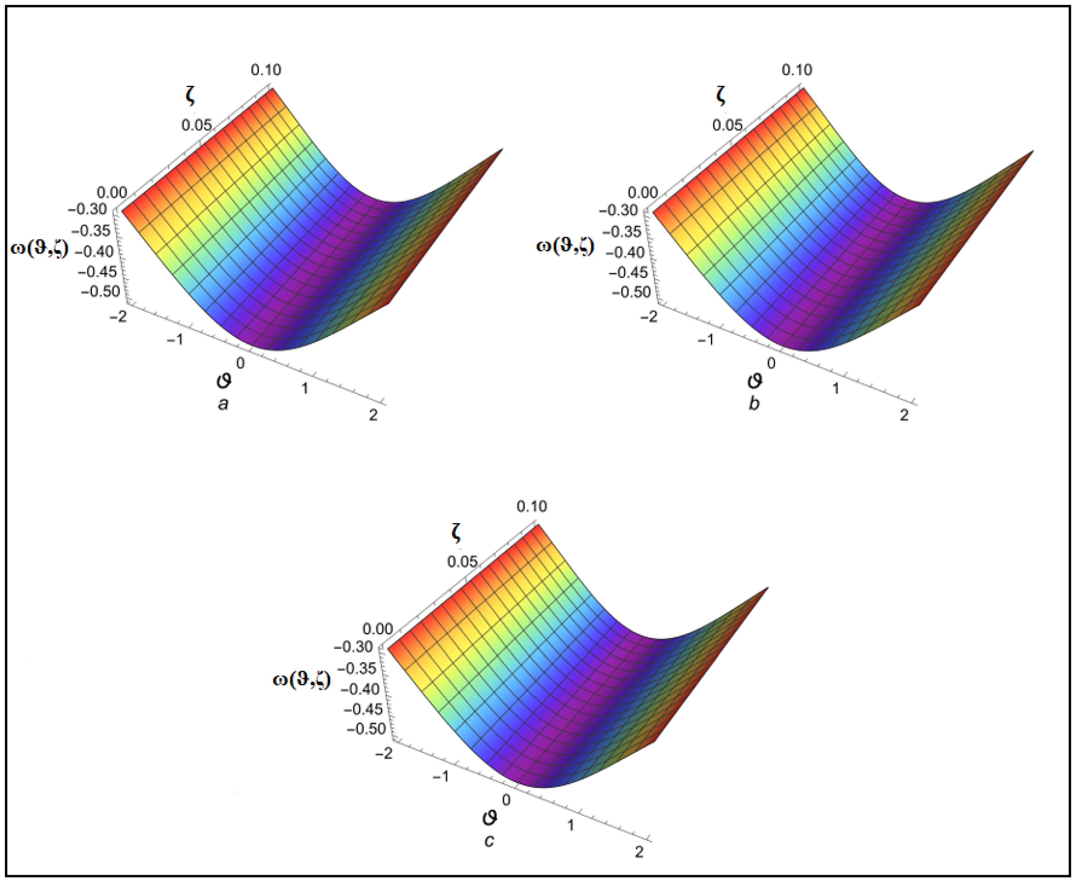
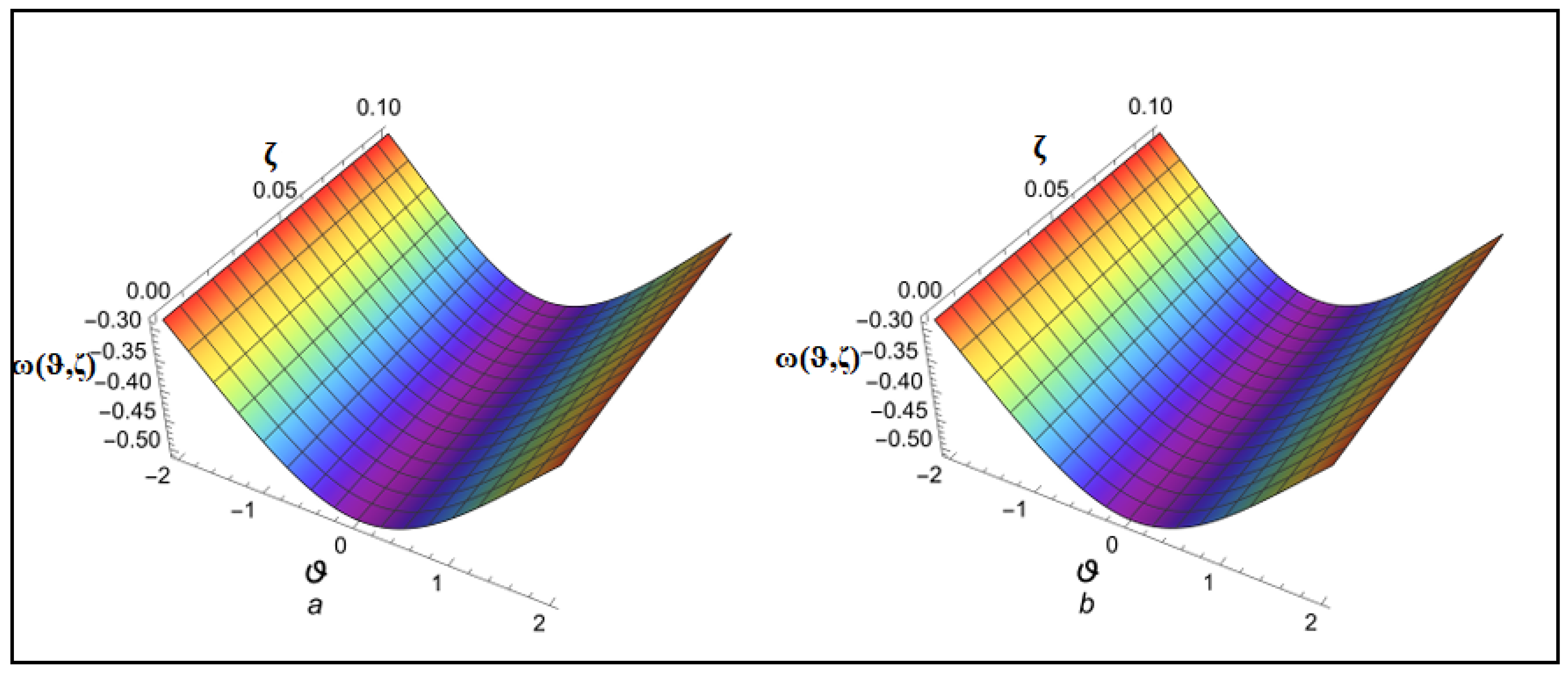
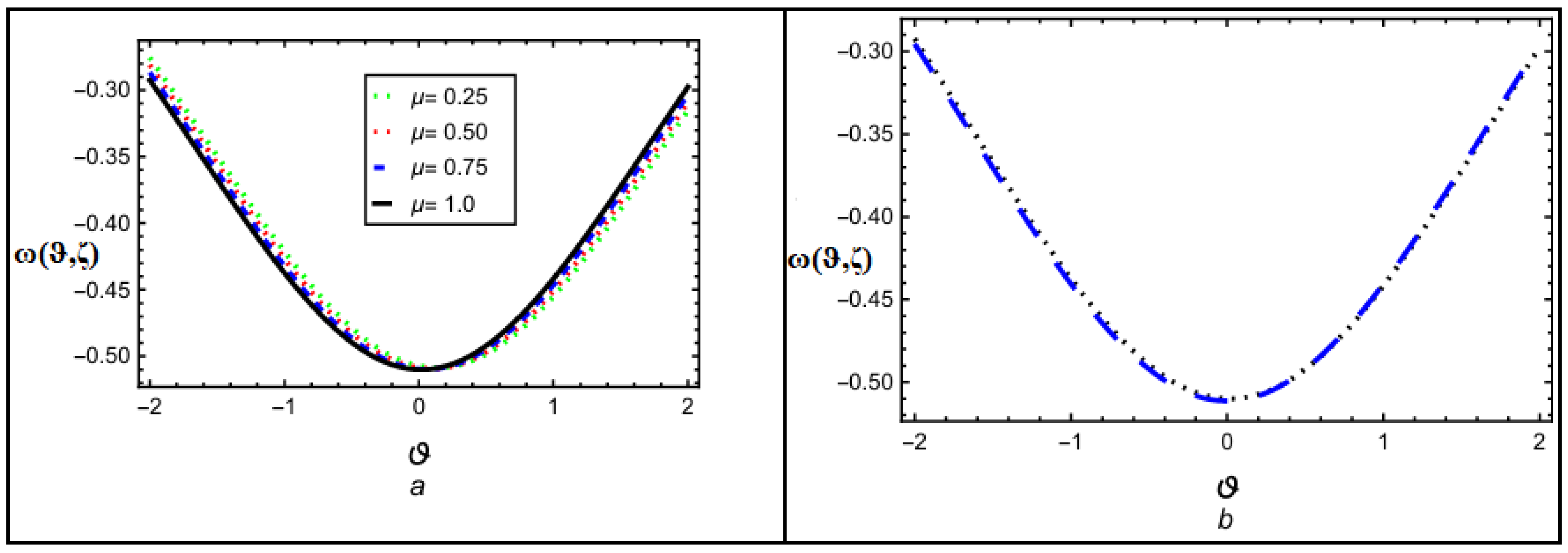
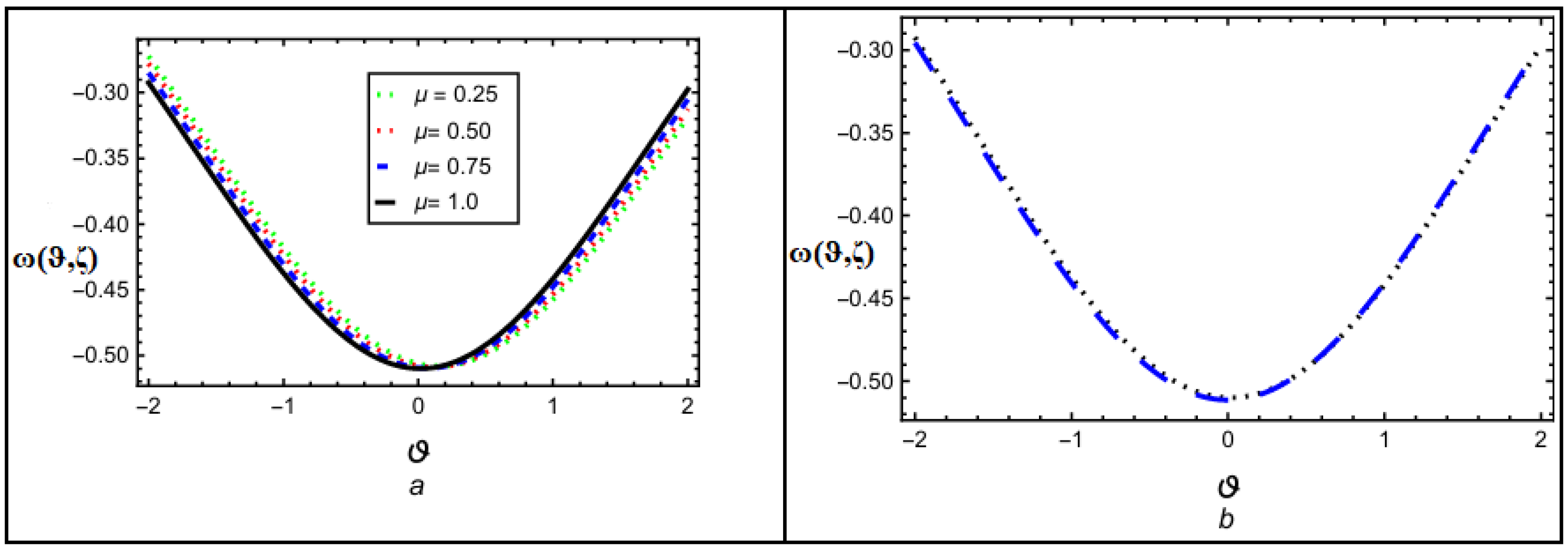
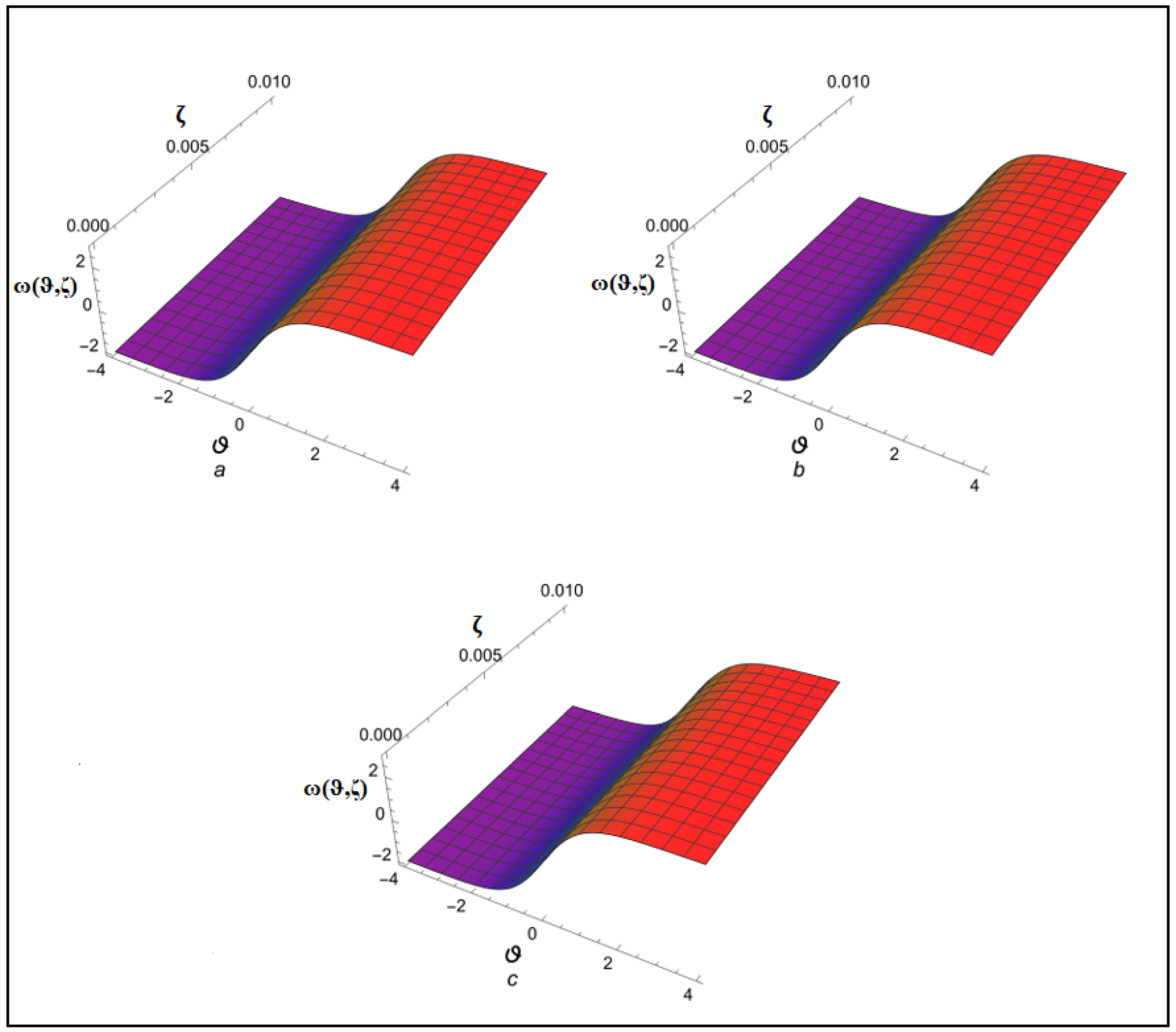
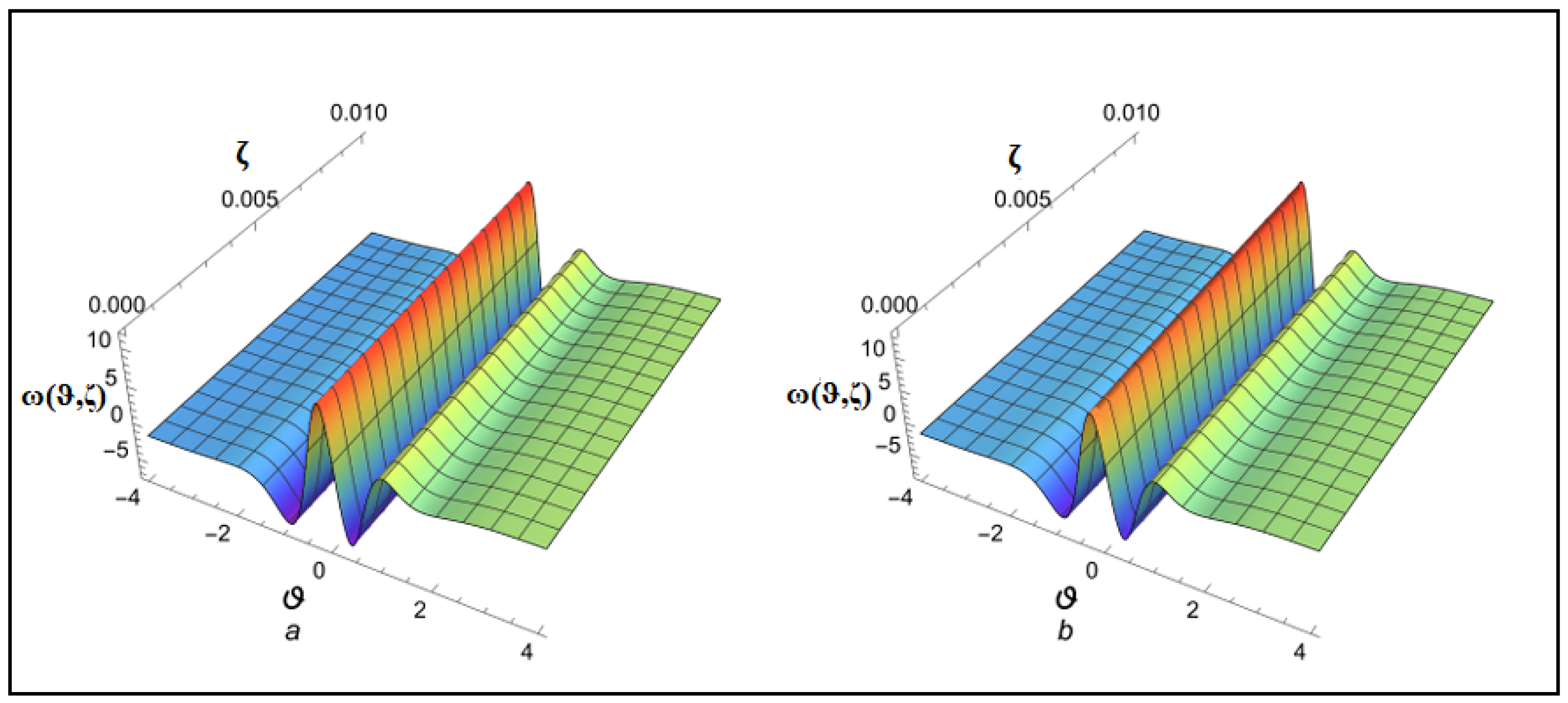
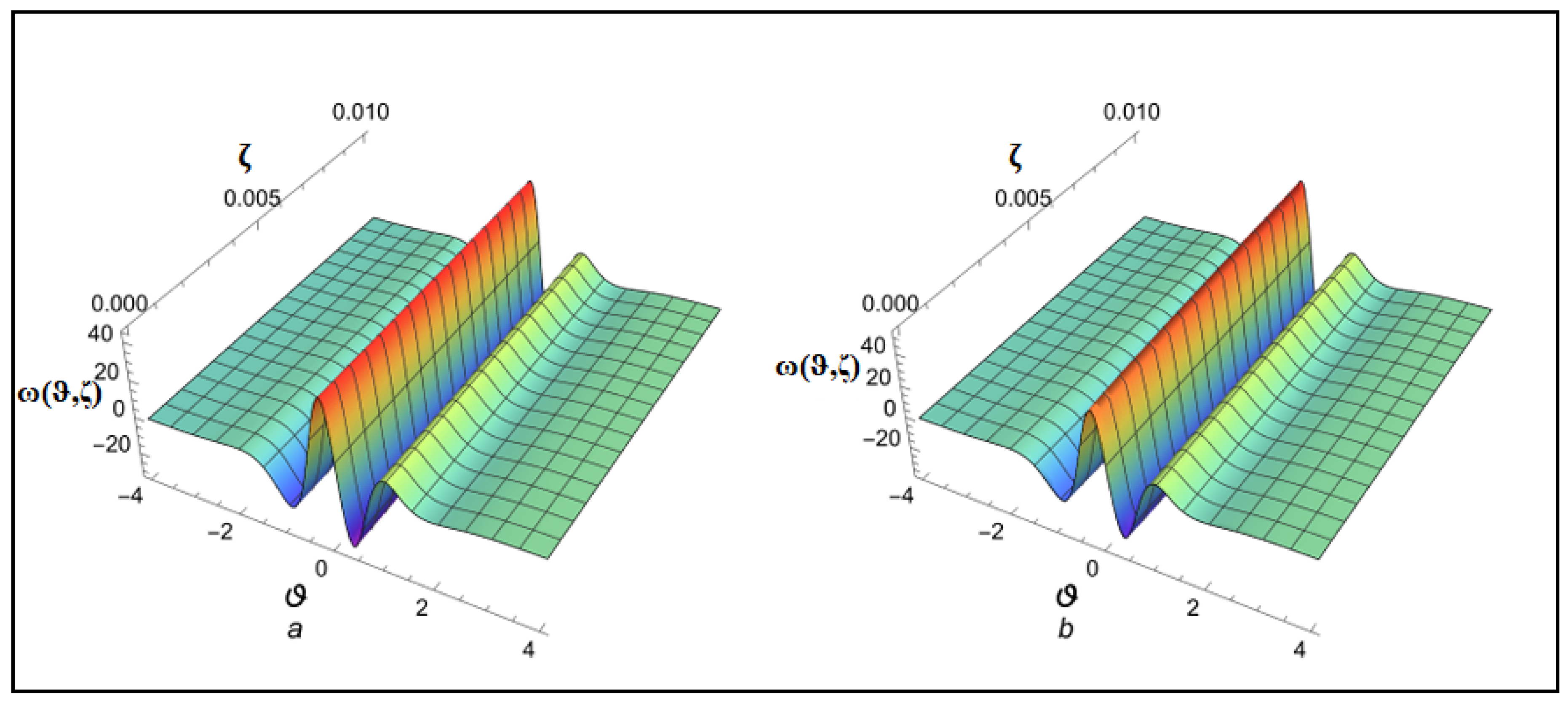
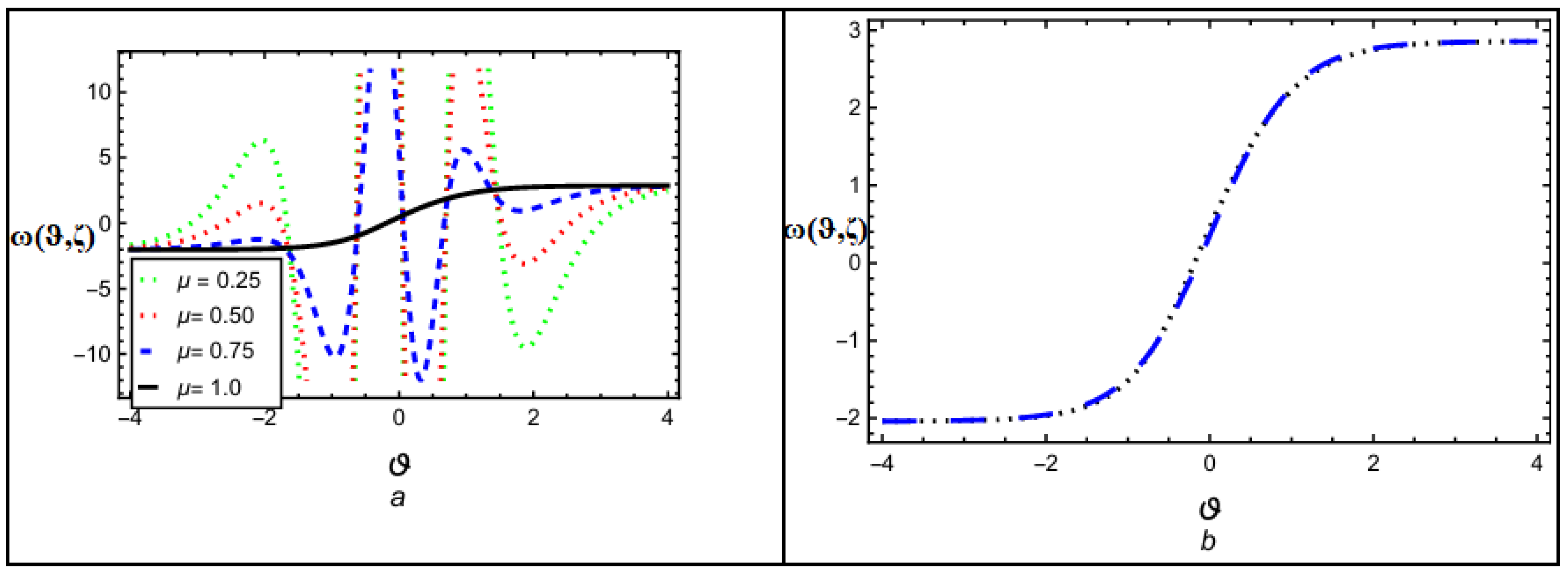
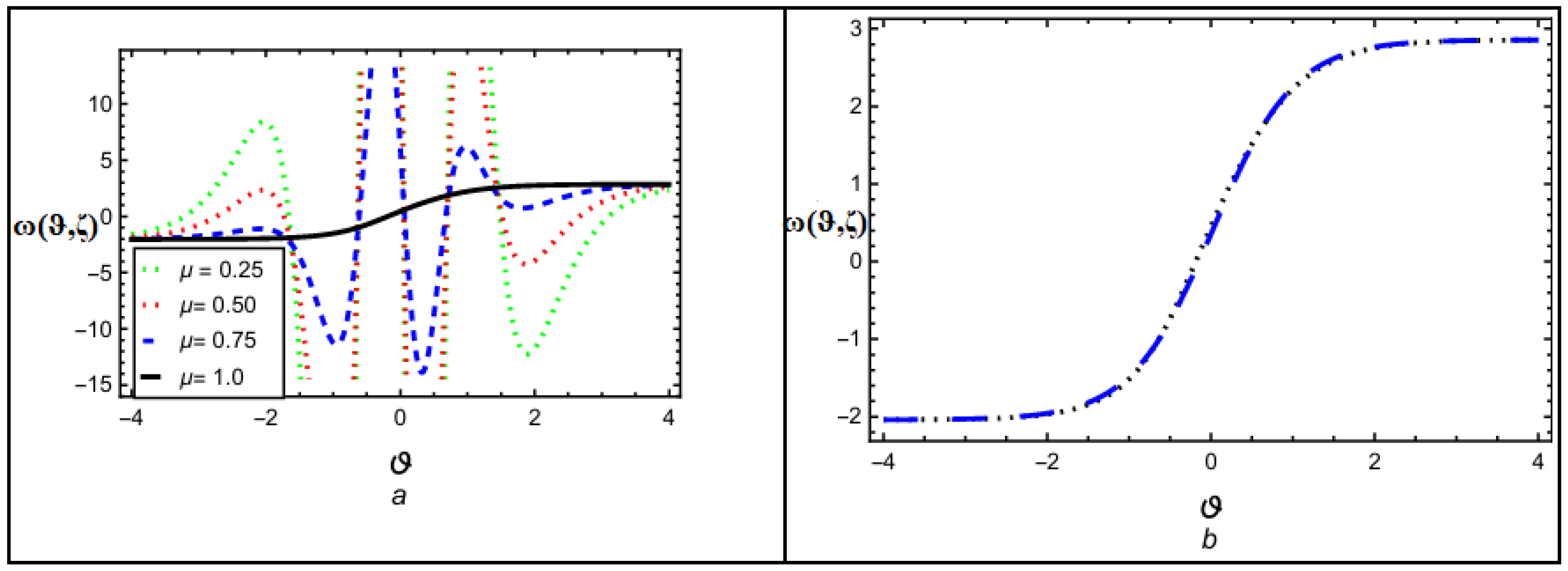
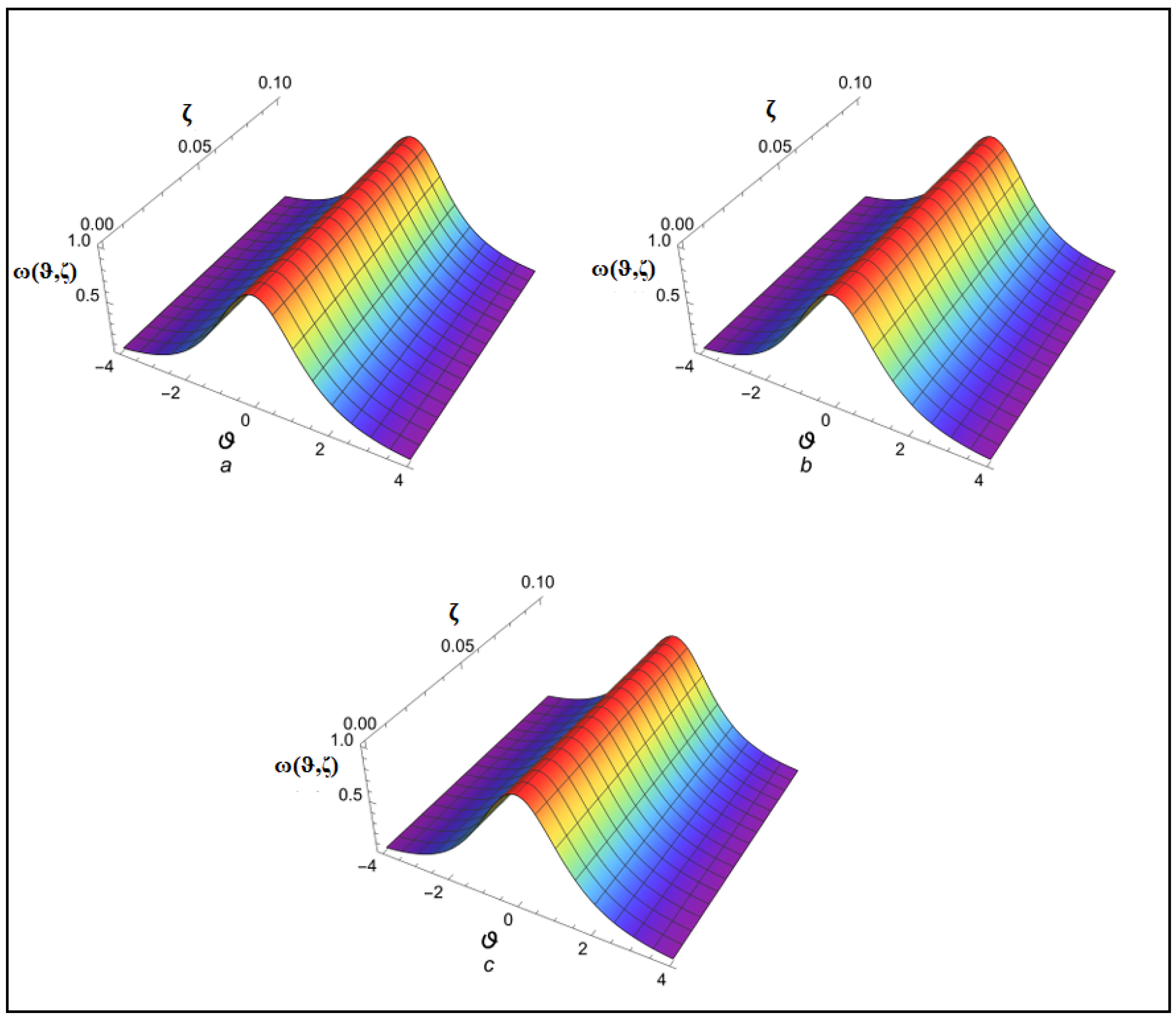
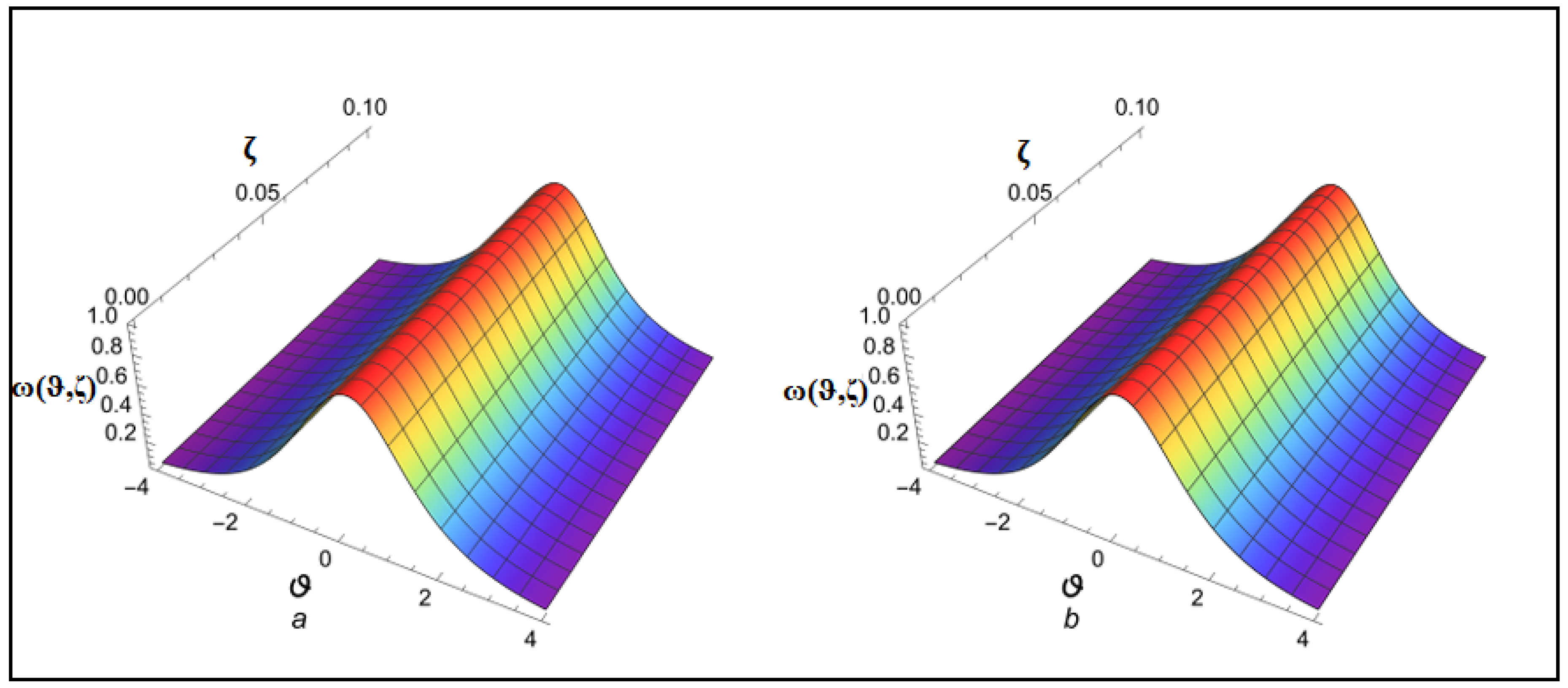
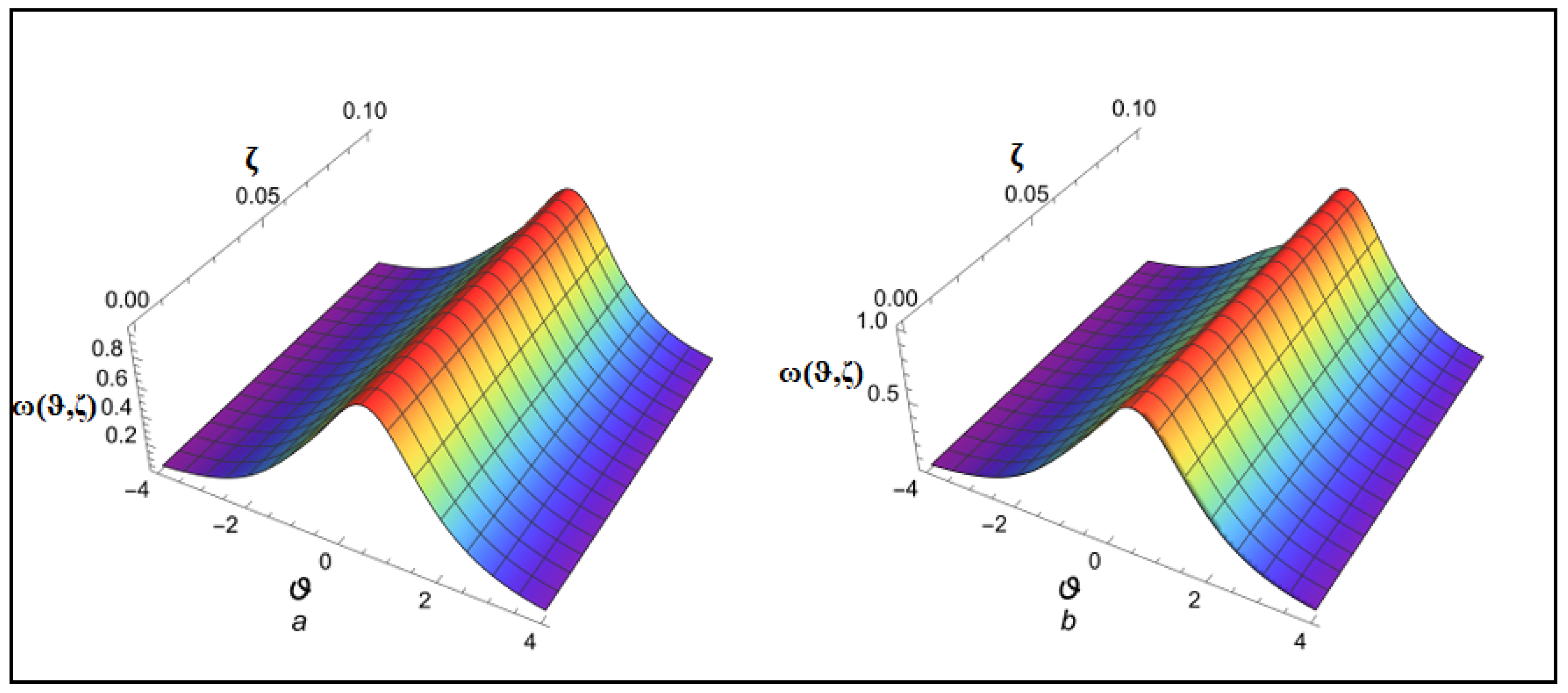
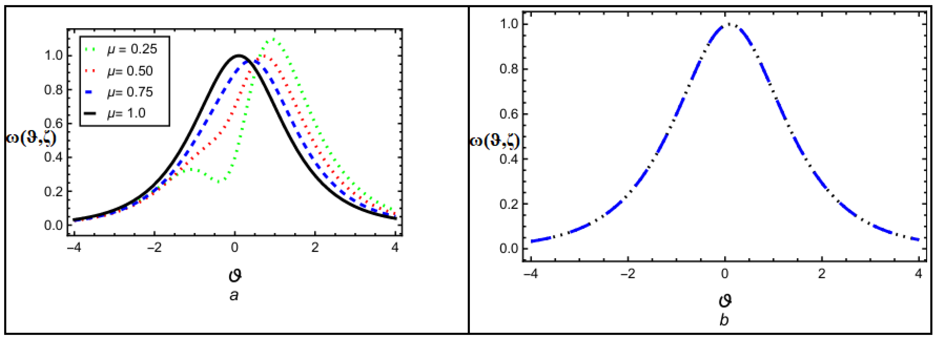
With the use of 2D and 3D simulations, the governing model’s physical interpretation is shown graphically. Using figures and tables, we compared the solutions from the suggested method with the precise solutions. The 3D simulations of the precise and suggested approach solutions for μ = 1 are shown in Figure 1. The 3D simulations of the suggested technique solutions for μ = 0.75 and μ = 0.50 are shown in Figure 2 and Figure 3. Similarly, the 2D simulations of the precise solution and the NTDM solution in terms of both operators are shown in Figure 4 and Figure 5. Figure 1, Figure 2, Figure 3, Figure 4 and Figure 5 demonstrate that fractional values of μ will result in smooth solution curves, whereas μ 1 will result in a solution curve that approaches the integer-order solution. The accurate and derived results for various μ values are shown in Table 1. The figures and tables further show that both derivative solutions converge to the exact result as the fractional order gets closer to 1. Additionally, the absolute errors of the suggested method solution and the outcomes obtained by ITM and RPSTM are compared in Table 2. This implies that the solutions generated by NTDM are better suited than those generated by ITM and RPSTM. Interestingly, the fractional-order situation gives wave profiles a damping-like quality that provides further modeling flexibility for physical systems with memory effects and anomalous diffusion.
Example 2. 
Assume fractional KdV Burger’s equation of the form [37]:
D ζ μ ω ( ϑ , ζ ) + ω ϑ ϑ ϑ ( ϑ , ζ ) + ω ϑ ϑ ( ϑ , ζ ) + ω 2 ( ϑ , ζ ) ω ϑ ( ϑ , ζ ) = 0 , 0 < μ 1 ,
with
ω ( ϑ , 0 ) = 6 ( exp ( ϑ ) exp ( ϑ ) ) ( exp ( ϑ ) + exp ( ϑ ) ) + 6 6 .
On inserting NT to Equation (55), we get
N [ D ζ μ ω ( ϑ , ζ ) ] = N ω ϑ ϑ ϑ ( ϑ , ζ ) N ω ϑ ϑ ( ϑ , ζ ) N ω 2 ( ϑ , ζ ) ω ϑ ( ϑ , ζ ) .
Now by using transform property
N [ ω ( ϑ , ζ ) ] = ω ( ϑ , 0 ) λ + N ω ϑ ϑ ϑ ( ϑ , ζ ) ω ϑ ϑ ( ϑ , ζ ) ω 2 ( ϑ , ζ ) ω ϑ ( ϑ , ζ ) .
On inserting inverse inverse NT, we have
ω ( ϑ , ζ ) = 6 ( exp ( ϑ ) exp ( ϑ ) ) ( exp ( ϑ ) + exp ( ϑ ) ) + 6 6 N 1 [ η λ μ N { ω ϑ ϑ ϑ ( ϑ , ζ ) + ω ϑ ϑ ( ϑ , ζ ) + ω 2 ( ϑ , ζ ) ω ϑ ( ϑ , ζ ) } ] .
  • Implementation of  N T D M C F
The series solution of ω ( ϑ , ζ ) is represented as
ω ( ϑ , ζ ) = l = 0 ω l ( ϑ , ζ ) .
The nonlinear term is indicated as ω 2 ω ϑ = l = 0 A l , So Equation (59) is taken as
l = 0 ω l + 1 ( ϑ , ζ ) = 6 ( exp ( ϑ ) exp ( ϑ ) ) ( exp ( ϑ ) + exp ( ϑ ) ) + 6 6 N 1 η ( λ μ ( λ η ) ) λ 2 N ω ϑ ϑ ϑ ( ϑ , ζ ) + ω ϑ ϑ ( ϑ , ζ ) + l = 0 A l .
The Adomian polynomials are calculated as stated in Equation (45). By comparison of both sides of Equation (61), we get
ω 0 ( ϑ , ζ ) = 6 ( exp ( ϑ ) exp ( ϑ ) ) ( exp ( ϑ ) + exp ( ϑ ) ) + 6 6 ,
ω 1 ( ϑ , ζ ) = 2 3 6 ( 61 exp ( 4 ϑ ) 166 exp ( 2 ϑ ) + 61 ) exp ( 2 ϑ ) ( exp ( 2 ϑ ) + 1 ) 4 μ ( ζ 1 ) + 1 ,
ω 2 ( ϑ , ζ ) = 2 9 ( exp ( 2 ϑ ) + 1 ) 7 ( ( 3721 exp ( 10 ϑ ) 93669 exp ( 8 ϑ ) + 421010 exp ( 6 ϑ ) 448658 exp ( 4 ϑ ) + 107493 exp ( 2 ϑ ) 3721 ) exp ( 2 ϑ ) 6 ) ( 1 μ ) 2 + 2 μ ( 1 μ ) ζ + μ 2 ζ 2 2 .
Lastly, the solution in N T D M C F manner is as follows:
ω ( ϑ , ζ ) = l = 0 ω l ( ϑ , ζ ) = ω 0 ( ϑ , ζ ) + ω 1 ( ϑ , ζ ) + ω 2 ( ϑ , ζ ) + , ω ( ϑ , ζ ) = 6 ( exp ( ϑ ) exp ( ϑ ) ) ( exp ( ϑ ) + exp ( ϑ ) ) + 6 6 2 3 6 ( 61 exp ( 4 ϑ ) 166 exp ( 2 ϑ ) + 61 ) exp ( 2 ϑ ) ( exp ( 2 ϑ ) + 1 ) 4 μ ( ζ 1 ) + 1 2 9 ( exp ( 2 ϑ ) + 1 ) 7 ( ( 3721 exp ( 10 ϑ ) 93669 exp ( 8 ϑ ) + 421010 exp ( 6 ϑ ) 448658 exp ( 4 ϑ ) + 107493 exp ( 2 ϑ ) 3721 ) exp ( 2 ϑ ) 6 ) ( 1 μ ) 2 + 2 μ ( 1 μ ) ζ + μ 2 ζ 2 2 + .
  • Implementation of  N T D M A B C
The series solution of ω ( ϑ , ζ ) is represented as
ω ( ϑ , ζ ) = l = 0 ω l ( ϑ , ζ ) .
The nonlinear term is indicated as ω 2 ω ϑ = l = 0 A l , So Equation (59) is taken as
l = 0 ω l + 1 ( ϑ , ζ ) = 6 ( exp ( ϑ ) exp ( ϑ ) ) ( exp ( ϑ ) + exp ( ϑ ) ) + 6 6 N 1 η μ ( λ μ + μ ( η μ λ μ ) ) λ 2 μ N ω ϑ ϑ ϑ ( ϑ , ζ ) + ω ϑ ϑ ( ϑ , ζ ) + l = 0 A l .
The Adomian polynomials are calculated as stated in Equation (45). By comparison of both sides of Equation (66) as
ω 0 ( ϑ , ζ ) = 6 ( exp ( ϑ ) exp ( ϑ ) ) ( exp ( ϑ ) + exp ( ϑ ) ) + 6 6 ,
ω 1 ( ϑ , ζ ) = 2 3 6 ( 61 exp ( 4 ϑ ) 166 exp ( 2 ϑ ) + 61 ) exp ( 2 ϑ ) ( exp ( 2 ϑ ) + 1 ) 4 1 μ + μ ζ μ Γ ( μ + 1 ) ,
ω 2 ( ϑ , ζ ) = 2 9 ( exp ( 2 ϑ ) + 1 ) 7 ( ( 3721 exp ( 10 ϑ ) 93669 exp ( 8 ϑ ) + 421010 exp ( 6 ϑ ) 448658 exp ( 4 ϑ ) + 107493 exp ( 2 ϑ ) 3721 ) exp ( 2 ϑ ) 6 ) μ 2 ζ 2 μ Γ ( 2 μ + 1 ) + 2 μ ( 1 μ ) ζ μ Γ ( μ + 1 ) + ( 1 μ ) 2 .
Lastly, the solution in N T D M A B C manner is as follows:
ω ( ϑ , ζ ) = l = 0 ω l ( ϑ , ζ ) = ω 0 ( ϑ , ζ ) + ω 1 ( ϑ , ζ ) + ω 2 ( ϑ , ζ ) + , ω ( ϑ , ζ ) = 6 ( exp ( ϑ ) exp ( ϑ ) ) ( exp ( ϑ ) + exp ( ϑ ) ) + 6 6 2 3 6 ( 61 exp ( 4 ϑ ) 166 exp ( 2 ϑ ) + 61 ) exp ( 2 ϑ ) ( exp ( 2 ϑ ) + 1 ) 4 1 μ + μ ζ μ Γ ( μ + 1 ) 2 9 ( exp ( 2 ϑ ) + 1 ) 7 ( ( 3721 exp ( 10 ϑ ) 93669 exp ( 8 ϑ ) + 421010 exp ( 6 ϑ ) 448658 exp ( 4 ϑ ) + 107493 exp ( 2 ϑ ) 3721 ) exp ( 2 ϑ ) 6 ) [ μ 2 ζ 2 μ Γ ( 2 μ + 1 ) + 2 μ ( 1 μ ) ζ μ Γ ( μ + 1 ) + ( 1 μ ) 2 ] + .
By taking μ = 1 , we get the exact solution as
ω ( ϑ , ζ ) = 6 ( exp ( ϑ 13 ζ 6 ) exp ( 13 ζ 6 ϑ ) ) ( exp ( ϑ + 13 ζ 6 ) + exp ( 13 ζ 6 ϑ ) ) + 6 6 .
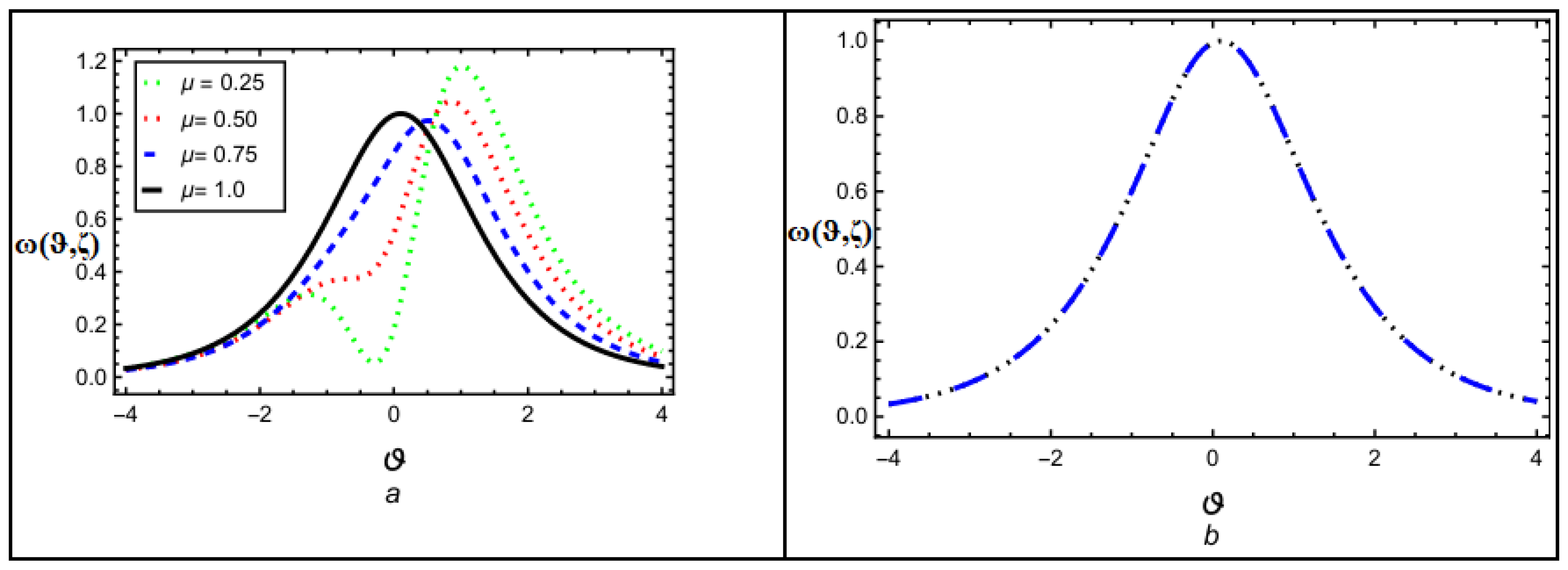
The 3D simulations of the precise and suggested approach solutions for μ = 1 are shown in Figure 6. The 3D simulations of the suggested technique solutions for μ = 0.75 and μ = 0.50 are shown in Figure 7 and Figure 8. Similarly, the 2D simulations of the precise solution and the NTDM solution in terms of both operators are shown in Figure 9 and Figure 10. The accurate and derived results for various μ values are shown in Table 3. A smoother profile that tends to achieve the classical solution at μ = 1 is generated by the fractional orders, which modify the solution amplitude and wave shape with lower values of μ . The figures and tables further show that both derivative solutions converge to the exact result as the fractional order gets closer to 1. Additionally, the absolute errors of the suggested method solution and the outcomes obtained by RPSTM are compared in Table 4. The fractional-order analysis generally shows that the dynamical representation of nonlinear PDEs can greatly benefit from the inclusion of the fractional order parameter μ .
Example 3. 
Assume fractional mKdV equation of the form [38]:
D ζ μ ω ( ϑ , ζ ) + 6 ω 2 ( ϑ , ζ ) ω ϑ ( ϑ , ζ ) + ω ϑ ϑ ϑ ( ϑ , ζ ) = 0 , 0 < μ 1 ,
with
ω ( ϑ , 0 ) = 2 ψ exp ( ψ ϑ ) exp ( 2 ψ ϑ ) + 1 .
On inserting NT to Equation (71), we get
N [ D ζ μ ω ( ϑ , ζ ) ] = N 6 ω 2 ( ϑ , ζ ) ω ϑ ( ϑ , ζ ) N ω ϑ ϑ ϑ ( ϑ , ζ ) .
Now by using transform property
N [ ω ( ϑ , ζ ) ] = ω ( ϑ , 0 ) λ + N 6 ω 2 ( ϑ , ζ ) ω ϑ ( ϑ , ζ ) ω ϑ ϑ ϑ ( ϑ , ζ ) .
On inserting inverse inverse NT, we have
ω ( ϑ , ζ ) = 2 ψ exp ( ψ ϑ ) exp ( 2 ψ ϑ ) + 1 N 1 η λ μ N 6 ω 2 ( ϑ , ζ ) ω ϑ ( ϑ , ζ ) + ω ϑ ϑ ϑ ( ϑ , ζ ) .
  • Implementation of  N T D M C F
The series solution of ω ( ϑ , ζ ) is represented as
ω ( ϑ , ζ ) = l = 0 ω l ( ϑ , ζ ) .
The nonlinear term is indicated as ω 2 ω ϑ = l = 0 A l , So Equation (75) is taken as
l = 0 ω l + 1 ( ϑ , ζ ) = 2 ψ exp ( ψ ϑ ) exp ( 2 ψ ϑ ) + 1 N 1 η ( λ μ ( λ η ) ) λ 2 N 6 l = 0 A l + ω ϑ ϑ ϑ ( ϑ , ζ ) .
The Adomian polynomials are calculated as stated in Equation (45). By comparing both sides of Equation (77), we get
ω 0 ( ϑ , ζ ) = 2 ψ exp ( ψ ϑ ) exp ( 2 ψ ϑ ) + 1 ,
ω 1 ( ϑ , ζ ) = 2 ψ 4 exp ( ψ ϑ ) ( exp ( 2 ψ ϑ ) 1 ) ( exp ( 2 ψ ϑ ) + 1 ) 2 μ ( ζ 1 ) + 1 ,
ω 2 ( ϑ , ζ ) = 2 ψ 7 exp ( ψ ϑ ) ( exp ( 4 ψ ϑ ) 6 exp ( 2 ψ ϑ ) 1 ) ( exp ( 2 ψ ϑ ) + 1 ) 3 ( 1 μ ) 2 + 2 μ ( 1 μ ) ζ + μ 2 ζ 2 2 .
Lastly, the solution in N T D M C F manner is as follows:
ω ( ϑ , ζ ) = l = 0 ω l ( ϑ , ζ ) = ω 0 ( ϑ , ζ ) + ω 1 ( ϑ , ζ ) + ω 2 ( ϑ , ζ ) + , ω ( ϑ , ζ ) = 2 ψ exp ( ψ ϑ ) exp ( 2 ψ ϑ ) + 1 2 ψ 4 exp ( ψ ϑ ) ( exp ( 2 ψ ϑ ) 1 ) ( exp ( 2 ψ ϑ ) + 1 ) 2 μ ( ζ 1 ) + 1 2 ψ 7 exp ( ψ ϑ ) ( exp ( 4 ψ ϑ ) 6 exp ( 2 ψ ϑ ) 1 ) ( exp ( 2 ψ ϑ ) + 1 ) 3 ( 1 μ ) 2 + 2 μ ( 1 μ ) ζ + μ 2 ζ 2 2 + .
  • Implementation of  N T D M A B C
The series solution of ω ( ϑ , ζ ) is represented as
ω ( ϑ , ζ ) = l = 0 ω l ( ϑ , ζ ) .
The nonlinear term is indicated as ω 2 ω ϑ = l = 0 A l , So Equation (75) is taken as
l = 0 ω l + 1 ( ϑ , ζ ) = 2 ψ exp ( ψ ϑ ) exp ( 2 ψ ϑ ) + 1 N 1 η μ ( λ μ μ ( λ μ η μ ) ) λ 2 μ N 6 l = 0 A l + ω ϑ ϑ ϑ ( ϑ , ζ ) .
The Adomian polynomials are calculated as stated in Equation (45). By comparing both sides of Equation (82), we get
ω 0 ( ϑ , ζ ) = 2 ψ exp ( ψ ϑ ) exp ( 2 ψ ϑ ) + 1 ,
ω 1 ( ϑ , ζ ) = 2 ψ 4 exp ( ψ ϑ ) ( exp ( 2 ψ ϑ ) 1 ) ( exp ( 2 ψ ϑ ) + 1 ) 2 1 μ + μ ζ μ Γ ( μ + 1 ) ,
ω 2 ( ϑ , ζ ) = 2 ψ 7 exp ( ψ ϑ ) ( exp ( 4 ψ ϑ ) 6 exp ( 2 ψ ϑ ) 1 ) ( exp ( 2 ψ ϑ ) + 1 ) 3 μ 2 ζ 2 μ Γ ( 2 μ + 1 ) + 2 μ ( 1 μ ) ζ μ Γ ( μ + 1 ) + ( 1 μ ) 2 .
Lastly, the solution in N T D M A B C manner is as follows:
ω ( ϑ , ζ ) = l = 0 ω l ( ϑ , ζ ) = ω 0 ( ϑ , ζ ) + ω 1 ( ϑ , ζ ) + ω 2 ( ϑ , ζ ) + , ω ( ϑ , ζ ) = 2 ψ exp ( ψ ϑ ) exp ( 2 ψ ϑ ) + 1 2 ψ 4 exp ( ψ ϑ ) ( exp ( 2 ψ ϑ ) 1 ) ( exp ( 2 ψ ϑ ) + 1 ) 2 1 μ + μ ζ μ Γ ( μ + 1 ) 2 ψ 7 exp ( ψ ϑ ) ( exp ( 4 ψ ϑ ) 6 exp ( 2 ψ ϑ ) 1 ) ( exp ( 2 ψ ϑ ) + 1 ) 3 μ 2 ζ 2 μ Γ ( 2 μ + 1 ) + 2 μ ( 1 μ ) ζ μ Γ ( μ + 1 ) + ( 1 μ ) 2 + .
By taking μ = 1 , we get the exact solution as
ω ( ϑ , ζ ) = 2 ψ exp ( ψ ( ϑ ψ 2 ζ ) ) exp ( 2 ψ ( ϑ ψ 2 ζ ) ) + 1 .
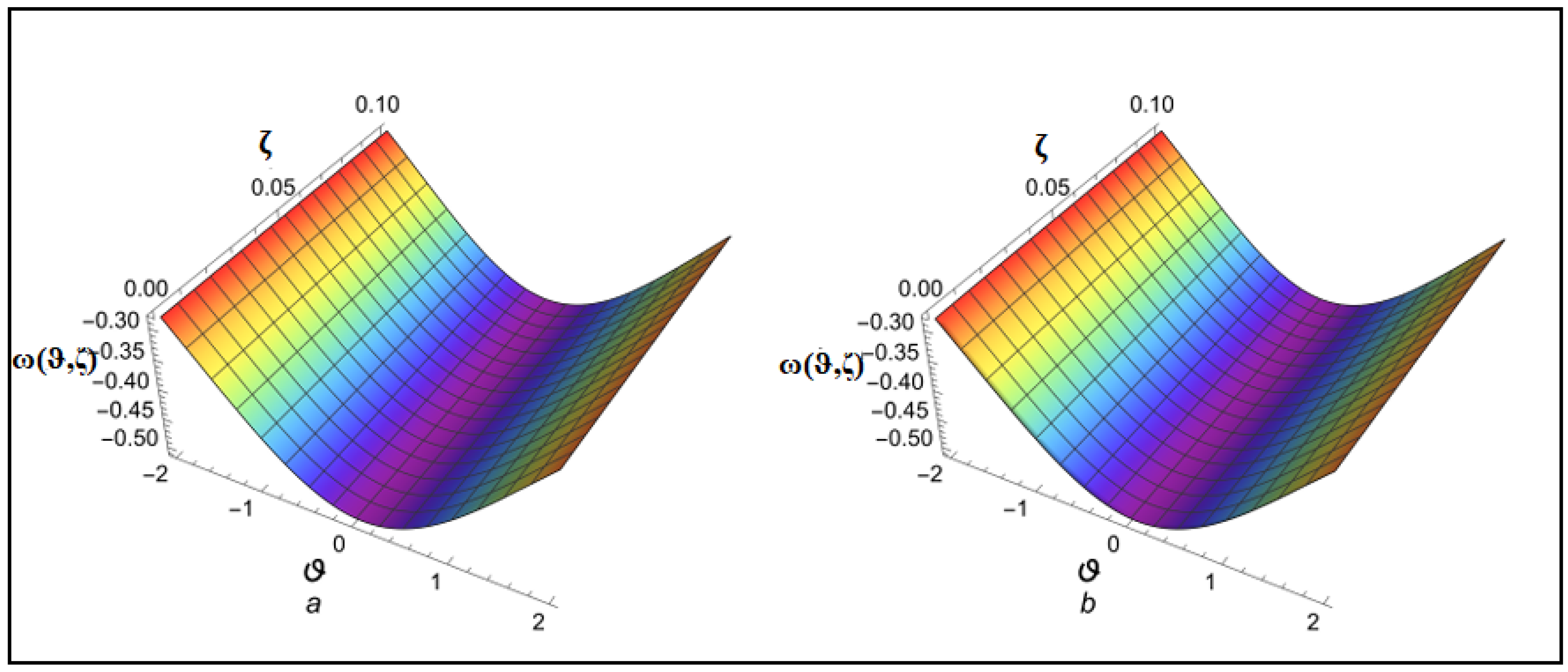
The 3D simulations of the precise and suggested approach solutions for μ = 1 are shown in Figure 11. The 3D simulations of the suggested technique solutions for μ = 0.75 and μ = 0.50 are shown in Figure 12 and Figure 13. Similarly, the 2D simulations of the precise solution and the suggested technique solution in terms of both operators are shown in Figure 14 and Figure 15. The accurate and derived results for various μ values are shown in Table 5. The tabular and graphical representations show how easy it is to apply NTDM and how it offers extremely valid and nearly accurate solutions. It is noteworthy that the formation of condensed soliton gas dynamics is mostly mediated by pairwise collisions of particle-like phenomena, such as breathers and solitary waves. These waves manifest as deep ocean waves, shallow groundwater waves, internal waves in a segmented sea, and fiber optics.

6. Conclusions

This work employs a novel methodology to offer the solutions to several nonlinear fractional KdV equations. The simplest and most effective method that may be used to solve FPDEs and associated systems is called NTDM. Each targeted problem’s fractional derivatives are represented by the Caputo–Fabrizio (CF) and Atangana–Baleanu derivative (ABC). After a discussion of the suggested technique for general nonlinear issues, a few nonlinear problems involving nonlinear FPDEs are resolved. Through the use of graphs and tables, the suggested technique results are presented. The comparison of the solutions revealed a very close correspondence between the precise and suggested approach solutions. More emphasis and important information about the dynamics of the targeted problems are offered by fractional order solutions. The fractional solutions are discovered to be convergent with the targeted problems actual solution. The current work supports the actual dynamics of physical processes in complete detail and can be expanded to include the solutions to other complex and nonlinear FPDEs and associated systems. To get better results, readers could combine our proposed approach with unique transforms and operators as a future study topic. We anticipate that this method will be used in the future to swiftly and efficiently tackle other fractional differential problems in scientific domains.

Author Contributions

Conceptualization, M.M.A. and R.A.; Methodology, M.M.A. and R.A.; Software, R.A.; Validation, M.M.A. and R.A.; Formal analysis, R.A.; Investigation, M.M.A. and R.A.; Resources, R.A.; Data curation, R.A.; Writing—original draft, M.M.A.; Writing—review & editing, R.A.; Visualization, M.M.A. and R.A.; Supervision, M.M.A.; Project administration, M.M.A. and R.A.; Funding acquisition, M.M.A. and R.A. All authors have read and agreed to the published version of the manuscript.

Funding

This study is funded by Prince Sattam bin Abdulaziz University under project number (PSAU/2025/01/36439).

Data Availability Statement

The numerical data used to support the findings of this study are included within the article.

Acknowledgments

The authors extend their appreciation to Prince Sattam bin Abdulaziz University for funding this research through the project number (PSAU/2025/01/36439).

Conflicts of Interest

The authors declare no conflicts of interest.

References

  1. Diethelm, K.; Ford, N.J. Analysis of fractional differential equations. J. Math. Anal. Appl. 2002, 265, 229–248. [Google Scholar] [CrossRef]
  2. Pandey, H.R.; Phaijoo, G.R. A Comprehensive Study of Fractional-Order Derivative and Their Interplay with Basic Functions. J. Nepal Math. Soc. 2024, 6, 38–52. [Google Scholar] [CrossRef]
  3. Pariyar, S.; Kafle, J. Caputo-Fabrizio approach to numerical fractional derivatives. BIBECHANA 2023, 20, 126–133. [Google Scholar] [CrossRef]
  4. Deressa, C.T. On the chaotic nature of the Rabinovich system through Caputo and Atangana–Baleanu–Caputo fractional derivatives. Adv. Contin. Discret. Model. 2022, 2022, 66. [Google Scholar] [CrossRef]
  5. Agbata, B.C.; Dervishi, R.; Gümxuxş, M.; Smerat, A.; Mbah, G.C.E. Analysis of fractional-order model for the transmission dynamics of malaria via Caputo–Fabrizio and Atangana–Baleanu operators. Sci. Rep. 2025, 15, 36359. [Google Scholar] [CrossRef]
  6. Okposo, N.I.; Adewole, M.O.; Okposo, E.N.; Ojarikre, H.I.; Abdullah, F.A. A mathematical study on a fractional COVID-19 transmission model within the framework of nonsingular and nonlocal kernel. Chaos Solitons Fractals 2021, 152, 111427. [Google Scholar] [CrossRef]
  7. Xu, C.; Farman, M.; Shehzad, A. Analysis and chaotic behavior of a fish farming model with singular and non-singular kernel. Int. J. Biomath. 2025, 18, 2350105. [Google Scholar] [CrossRef]
  8. Xua, C.; Liaob, M.; Farman, M.; Shehzade, A. Hydrogenolysis of glycerol by heterogeneous catalysis: A fractional order kinetic model with analysis. MATCH Commun. Math. Comput. Chem. 2024, 91, 635–664. [Google Scholar] [CrossRef]
  9. Abro, K.A.; Memon, A.A.; Uqaili, M.A. A comparative mathematical analysis of RL and RC electrical circuits via Atangana-Baleanu and Caputo-Fabrizio fractional derivatives. Eur. Phys. J. Plus 2018, 133, 113. [Google Scholar] [CrossRef]
  10. Ahmad, S.; Saifullah, S. Analysis of the seventh-order Caputo fractional KdV equation: Applications to the Sawada–Kotera–Ito and Lax equations. Commun. Theor. Phys. 2023, 75, 085002. [Google Scholar] [CrossRef]
  11. Abro, K.A.; Chandio, A.D.; Abro, I.A.; Khan, I. Dual thermal analysis of magnetohydrodynamic flow of nanofluids via modern approaches of Caputo–Fabrizio and Atangana–Baleanu fractional derivatives embedded in porous medium. J. Therm. Anal. Calorim. 2019, 135, 2197–2207. [Google Scholar] [CrossRef]
  12. Xu, C.; Zhao, Y.; Lin, J.; Pang, Y.; Liu, Z.; Shen, J.; Liao, M.; Li, P.; Qin, Y. Bifurcation investigation and control scheme of fractional neural networks owning multiple delays. Comput. Appl. Math. 2024, 43, 186. [Google Scholar] [CrossRef]
  13. Chauhan, J.P.; Khirsariya, S.R.; Hathiwala, G.S.; Biswas Hathiwala, M. New analytical technique to solve fractional-order Sharma–Tasso–Olver differential equation using Caputo and Atangana–Baleanu derivative operators. J. Appl. Anal. 2024, 30, 1–16. [Google Scholar] [CrossRef]
  14. Kilbas, A.A.; Srivastava, H.M.; Trujillo, J.J. Theory and Applications of Fractional Differential Equations; Elsevier Science B.V.: Amsterdam, The Netherlands, 2006; Volume 204. [Google Scholar]
  15. Abbas, S.; Benchohra, M.; N’Guerekata, G.M. Advanced Fractional Differential and Integral Equations; Nova Publishers: Hauppauge, NY, USA, 2015. [Google Scholar]
  16. Legnani, W.; Moschandreou, T.E.; Reyhanoglu, M. Nonlinear Systems: Theoretical Aspects and Recent Applications; IntechOpen: London, UK, 2020. [Google Scholar]
  17. Hilfer, R. Applications of Fractional Calculus in Physics; River Edge, World Scientific Publishing Co.: Singapore, 2000. [Google Scholar]
  18. Hernández, E.; O’Regan, D.; Balachandran, K. On recent developments in the theory of abstract differential equations with fractional derivatives. Nonlinear Anal. Theory Methods Appl. 2010, 73, 3462–3471. [Google Scholar] [CrossRef]
  19. Magin, R.; Ortigueira, M.D.; Podlubny, I.; Trujillo, J.J. On the fractional signals and systems. Signal Process 2011, 91, 350–371. [Google Scholar] [CrossRef]
  20. Mainardi, F. Fractional Calculus and Waves in Linear Viscoelasticity: An Introduction to Mathematical Models; Imperial College Press: London, UK, 2010. [Google Scholar]
  21. Arafa, A.A. Analytical solutions for nonlinear fractional physical problems via natural homotopy perturbation method. Int. J. Appl. Comput. Math. 2021, 7, 179. [Google Scholar] [CrossRef]
  22. Qureshi, S.; Yusuf, A. A new third order convergent numerical solver for continuous dynamical systems. J. King Saud Univ.-Sci. 2020, 32, 1409–1416. [Google Scholar] [CrossRef]
  23. Pavani, K.; Raghavendar, K.; Aruna, K. Soliton solutions of the time-fractional Sharma–Tasso–Olver equations arise in nonlinear optics. Opt. Quantum Electron. 2024, 56, 748. [Google Scholar] [CrossRef]
  24. AlBaidani, M.M. Analytical Insight into Some Fractional Nonlinear Dynamical Systems Involving the Caputo Fractional Derivative Operator. Fractal Fract. 2025, 9, 320. [Google Scholar] [CrossRef]
  25. Bushnaq, S.; Ali, A. Numerical investigation of fractional Fisher partial differential equation via natural transform decomposition method. Partial Differ. Equations Appl. Math. 2024, 9, 100642. [Google Scholar] [CrossRef]
  26. AlBaidani, M.M.; Alzahrani, R. Novel approximations to the non-linear fractional Belousov-Zhabotinsky reaction in the frame of Caputo operator. Bound. Value Probl. 2026, 2026, 36. [Google Scholar] [CrossRef]
  27. AlBaidani, M.M. Comparative Study of the Nonlinear Fractional Generalized Burger-Fisher Equations Using the Homotopy Perturbation Transform Method and New Iterative Transform Method. Fractal Fract. 2025, 9, 390. [Google Scholar] [CrossRef]
  28. Baeumer, B.; Benson, D.A.; Meerschaert, M.M.; Wheatcraft, S.W. Subordinated advection-dispersion equation for contaminant transport. Water Resour. Res. 2001, 37, 1543–1550. [Google Scholar] [CrossRef]
  29. Benson, D.A.; Wheatcraft, S.W.; Meerschaert, M.M. Application of a fractional advection-dispersion equation. Water Resour. Res. 2000, 36, 1403–1412. [Google Scholar] [CrossRef]
  30. Zhang, J.; Yin, L. Residual power series method for the time fractional Fornberg-Whitham equation. Int. J. Dyn. Syst. Differ. Equ. 2020, 10, 570–585. [Google Scholar] [CrossRef]
  31. Jassim, H.K.; Hussein, G.A.A. Analytical solutions to fractional differential equations: A comparative study with the natural homotopy pertutation method. AIP Conf. Proc. 2025, 3264, 050048. [Google Scholar]
  32. AlBaidani, M.M.; Alzahrani, R. A novel approach to solving generalised nonlinear dynamical systems within the Caputo operator. Fractal Fract. 2025, 9, 503. [Google Scholar] [CrossRef]
  33. Das, S.; Gupta, P.K. Homotopy analysis method for solving fractional hyperbolic partial differential equations. Int. J. Comput. Math. 2011, 88, 578–588. [Google Scholar] [CrossRef]
  34. Chen, Y.; Sun, Y.; Liu, L. Numerical solution of fractional partial differential equations with variable coefficients using generalized fractional-order Legendre functions. Appl. Math. Comput. 2014, 244, 847–858. [Google Scholar] [CrossRef]
  35. Nazari, D.; Shahmorad, S. Application of the fractional differential transform method to fractional-order integro-differential equations with nonlocal boundary conditions. J. Comput. Appl. Math. 2010, 234, 883–891. [Google Scholar] [CrossRef]
  36. Baseri, A.; Babolian, E.; Abbasbandy, S. Normalized Bernstein polynomials in solving space-time fractional diffusion equation. Adv. Differ. Equ. 2017, 2017, 346. [Google Scholar] [CrossRef]
  37. Almusawa, M.Y.; Aldawsari, K.; Mshary, N. Fractional analysis of nonlinear dynamics in Korteweg-de Vries-Burgers’ and modified Korteweg-de Vries equations. Bound. Value Probl. 2025, 2025, 165. [Google Scholar] [CrossRef]
  38. Dong, Z. Construction of solitary wave solutions and rational solutions for mKdV equation with initial value problem by homotopy perturbation method. Open Access Libr. J. 2018, 5, 1. [Google Scholar] [CrossRef]
  39. Chen, Z.Y.; Huang, N.N.; Liu, Z.Z.; Xiao, Y. An explicit expression of the dark N-soliton solution of the MKdV equation by means of the Darboux transformation. J. Phys. A Math. Gen. 1993, 26, 1365. [Google Scholar] [CrossRef]
  40. Wazwaz, A.M. The extended tanh method for abundant solitary wave solutions of nonlinear wave equations. Appl. Math. Comput. 2007, 187, 1131–1142. [Google Scholar] [CrossRef]
  41. Parkes, E.J. Observations on the tanh-coth expansion method for finding solutions to nonlinear evolution equations. Appl. Math. Comput. 2010, 217, 1749–1754. [Google Scholar] [CrossRef]
  42. Trogdon, T.; Olver, S.; Deconinck, B. Numerical inverse scattering for the Korteweg-de Vries and modified Korteweg-de Vries equations. Phys. D Nonlinear Phenom. 2012, 241, 1003–1025. [Google Scholar] [CrossRef]
  43. Yin, J.L.; Xing, Q.Q.; Tian, L.X. Complex dynamical behaviors of compact solitary waves in the perturbed mKdV equation. Chin. Phys. B 2014, 23, 080201. [Google Scholar] [CrossRef]
  44. Xin, X.P.; Miao, Q.; Chen, Y. Nonlocal symmetry, optimal systems, and explicit solutions of the mKdV equation. Chin. Phys. B 2013, 23, 010203. [Google Scholar] [CrossRef]
  45. Abdallah, A.M.; Hussein, R.K.; Fadel, M.M. Unveiling the dualistic nature of the natural transform: Theoretical approaches. Nonlinear Sci. 2025, 6, 100090. [Google Scholar] [CrossRef]
  46. Adomian, G. A new approach to nonlinear partial differential equations. J. Math. Anal. Appl. 1984, 102, 420–434. [Google Scholar] [CrossRef]
  47. Alkan, A.; Anaç, H. The novel numerical solutions for time-fractional Fornberg-Whitham equation by using fractional natural transform decomposition method. AIMS Math. 2024, 9, 25333–25359. [Google Scholar] [CrossRef]
  48. Alzahrani, A.B.; Alhawael, G. Novel computations of the time-fractional coupled Korteweg–de Vries equations via non-singular kernel operators in terms of the natural transform. Symmetry 2023, 15, 2010. [Google Scholar] [CrossRef]
  49. Zhou, M.X.; Kanth, A.S.V.; Aruna, K.; Raghavendar, K.; Rezazadeh, H.; Inc, M.; Aly, A.A. Numerical Solutions of Time Fractional Zakharov-Kuznetsov Equation via Natural Transform Decomposition Method with Nonsingular Kernel Derivatives. J. Funct. Spaces 2021, 2021, 9884027. [Google Scholar] [CrossRef]
Figure 1. The surface demonstrating (a) the accurate, (b) N T D M C F and (c) N T D M A B C solutions for Example 1.
Symmetry 18 00391 g001
Figure 2. The surface demonstrating (a) N T D M C F and (b) N T D M A B C solution at μ = 0.75 .
Symmetry 18 00391 g002
Figure 3. The surface demonstrating (a) N T D M C F and (b) N T D M A B C solution at μ = 0.50 .
Symmetry 18 00391 g003
Figure 4. The surface demonstrating (a) N T D M C F solution at various μ orders and (b) showing comparison of N T D M C F with accurate solution at μ = 1 .
Symmetry 18 00391 g004
Figure 5. The surface demonstrating (a) N T D M A B C solution at various μ orders and (b) showing comparison of N T D M A B C with accurate solution at μ = 1 .
Symmetry 18 00391 g005
Figure 6. The surface demonstrating (a) the accurate, (b) N T D M C F and (c) N T D M A B C solutions for Example 2.
Symmetry 18 00391 g006
Figure 7. The surface demonstrating (a) N T D M C F and (b) N T D M A B C solution at μ = 0.75 .
Symmetry 18 00391 g007
Figure 8. The surface demonstrating (a) N T D M C F and (b) N T D M A B C solution at μ = 0.50 .
Symmetry 18 00391 g008
Figure 9. The surface demonstrating (a) N T D M C F solution at various μ orders and (b) showing comparison of N T D M C F with accurate solution at μ = 1 .
Symmetry 18 00391 g009
Figure 10. The surface demonstrating (a) N T D M A B C solution at various μ orders and (b) showing comparison of N T D M A B C with accurate solution at μ = 1 .
Symmetry 18 00391 g010
Figure 11. The surface demonstrating (a) the accurate, (b) N T D M C F and (c) N T D M A B C solutions for Example 3.
Symmetry 18 00391 g011
Figure 12. The surface demonstrating (a) N T D M C F and (b) N T D M A B C solution at μ = 0.75 .
Symmetry 18 00391 g012
Figure 13. The surface demonstrating (a) N T D M C F and (b) N T D M A B C solution at μ = 0.50 .
Symmetry 18 00391 g013
Figure 14. The surface demonstrating (a) N T D M C F solution at various μ orders and (b) showing comparison of N T D M C F with accurate solution at μ = 1 .
Symmetry 18 00391 g014
Figure 15. The surface demonstrating (a) N T D M A B C solution at various μ orders and (b) showing comparison of N T D M A B C with accurate solution at μ = 1 .
Symmetry 18 00391 g015
Table 1. Analysis of the accurate and proposed method solution.
ζ ϑ NTDM ABC at NTDM CF at NTDM ABC at NTDM CF at Exact at
μ = 0 . 99 μ = 0 . 99 μ = 1 μ = 1 μ = 1
0.00.29999995820.29999996000.29999999420.29999999420.2999999944
0.20.29936879350.29936860000.29936484440.29936484440.2999751640
0.40.29747171590.29747133070.29746385690.29746385690.2995938792
0.010.60.29434457800.29434400860.29433295660.29433295660.2979439296
0.80.29004536930.29004462590.29003019850.29003019850.2935639333
10.28465158290.28465067870.28463313160.28463313160.2846331317
0.00.29999986180.29999986920.29999994820.29999994820.2999999480
0.20.29937653680.29937608900.29937245430.29937245430.2999766534
0.40.29748715160.29748625700.29747897780.29747897780.2995999645
0.030.60.29436741650.29436609190.29435530490.29435530490.2979575664
0.80.29007519190.29007346170.29005936450.29005936450.2935876813
10.28468786100.28468575570.28466859840.28466859840.2846685983
0.00.29999971780.29999973330.29999985600.29999985600.2999998560
0.20.29938417620.29938353330.29938001850.29938001850.2999780972
0.40.29750242900.29750113990.29749405440.29749405440.2996060045
0.050.60.29439004510.29438813390.29437761090.29437761090.2979711590
0.80.29010475690.29010225890.29008849120.29008849120.2936113880
10.28472383800.28472079730.28470402930.28470402930.2847040293
Table 2. The comparison of our method solution with the ITM [37] and the RPSTM [37] at μ = 1 .
ζ ITM Error RPSTM Error NTDM ABC Error NTDM CF Error
0.12.0016544 × 10 5 1.9744012 × 10 5 2.3990000 × 10 7 2.3990000 × 10 7
0.27.7213786 × 10 5 7.6672159 × 10 5 1.7980000 × 10 7 1.7980000 × 10 7
0.31.6432297 × 10 4 1.6351377 × 10 4 1.1970000 × 10 7 1.1970000 × 10 7
0.42.6923314 × 10 4 2.6815863 × 10 4 5.9800000 × 10 8 5.9800000 × 10 8
0.53.7501932 × 10 4 3.7368249 × 10 4 0.00000000000000.0000000000000
0.64.6000623 × 10 4 4.5841080 × 10 4 5.9500000 × 10 8 5.9500000 × 10 8
0.74.9789793 × 10 4 4.9604829 × 10 4 1.1880000 × 10 7 1.1880000 × 10 7
0.84.5800758 × 10 4 4.5590880 × 10 4 1.7770000 × 10 7 1.7770000 × 10 7
0.93.0562718 × 10 4 3.0328498 × 10 4 2.3620000 × 10 7 2.3620000 × 10 7
1.02.5792975 × 10 6 2.9475186 × 10 7 2.9410000 × 10 7 2.9410000 × 10 7
Table 3. Analysis of the accurate and proposed method solution.
ζ ϑ NTDM ABC at NTDM CF at NTDM ABC at NTDM CF at Exact at
μ = 0 . 99 μ = 0 . 99 μ = 1 μ = 1 μ = 1
1.02.22397460502.22425988102.26852628702.26852628702.2715327840
1.52.58611619902.58638407702.62185889602.62185889602.6244387180
2.02.74948470702.74963598502.76800184202.76800184202.7692482160
0.0012.52.81652627302.81659183102.82430301102.82430301102.8248084610
3.02.84237339702.84239902802.84537955302.84537955302.8455722300
3.52.85205728102.85206692402.85318363702.85318363702.8532554480
1.02.21618347502.21687709402.25825908102.25825908102.2670454940
1.52.57865560702.57933534502.61477470002.61477470002.6225055120
2.02.74523195902.74562360302.76470113002.76470113002.7684920020
0.0032.52.81467745202.81484832902.82297660802.82297660802.8245237740
3.02.84164975402.84171672002.84487536702.84487536702.8454665980
3.52.85178491002.85181012702.85299590302.85299590302.8532164650
1.02.20875738202.20976997502.24827314102.24827314102.2625285960
1.52.57124521702.57228310702.60768692502.60768692502.6205571020
2.02.74092747302.74153742302.76132512602.76132512602.7677294490
0.0052.52.81279431402.81306217802.82160668902.82160668902.8242366420
3.02.84091104902.84101626402.84435265802.84435265802.8453600550
3.52.85150664502.85154629702.85280099702.85280099702.8531771460
Table 4. The comparison of our method solution with the RPSTM at μ = 1 .
ζ RPSTM Error NTDM ABC Error NTDM CF Error
1.02.6567180  ×   10 2 2.6567179   ×   10 2 2.6567179   ×   10 2
1.62.3155500   ×   10 2 2.3155499   ×   10 2 2.3155499   ×   10 2
2.29.4697320   ×   10 3 9.4697322   ×   10 3 9.4697322   ×   10 3
2.83.1283675   ×   10 3 3.1283658   ×   10 3 3.1283658   ×   10 3
3.49.6889137   ×   10 4 9.6889321   ×   10 4 9.6889321   ×   10 4
4.02.9428743   ×   10 4 2.9428659   ×   10 4 2.9428659   ×   10 4
4.68.8862376   ×   10 5 8.8862588   ×   10 5 8.8862588   ×   10 5
5.22.6785252   ×   10 5 2.6785170   ×   10 5 2.6785170   ×   10 5
5.88.0694165   ×   10 6 8.0710687   ×   10 6 8.0710687   ×   10 6
Table 5. Analysis of the accurate and proposed method solution.
ζ ϑ NTDM ABC at NTDM CF at NTDM ABC at NTDM CF at Exact at
μ = 0 . 99 μ = 0 . 99 μ = 1 μ = 1 μ = 1
0.010.00.99963706740.99965299500.99995000000.99995000000.9999500020
0.20.98394913930.98386482540.98221772580.98221772580.9822175738
0.40.93194192970.93177311150.92848911130.92848911130.9284888698
0.60.85266752130.85244209090.84806312520.84806312520.8480628778
0.80.75780151520.75754962860.75266050500.75266050500.7526603096
10.65816543970.65791199730.65299500340.65299500340.6529948774
0.030.00.99880035460.99886495500.99955000000.99955000000.9995501686
0.20.98715534700.98698363170.98572599820.98572599820.9857219806
0.40.93858891680.93821345200.93525504890.93525504890.9352485588
0.60.86164646630.86113076240.85698091470.85698091470.8569742204
0.80.76789549750.76731074060.76255518540.76255518540.7625498584
10.66835976930.66776611050.66290757910.66290757910.6629041338
0.050.00.99755070860.99768487500.99875000000.99875000000.9987513004
0.20.98995953760.98974805490.98887269180.98887269180.9888545122
0.40.94491200350.94439585500.94175781180.94175781180.9417279294
0.60.87041070630.86967949410.86575592280.86575592280.8657248512
0.80.77787924730.77703723120.77241454120.77241454120.7723896738
10.67852360100.67766088680.67286164360.67286164360.6728454780
Disclaimer/Publisher’s Note: The statements, opinions and data contained in all publications are solely those of the individual author(s) and contributor(s) and not of MDPI and/or the editor(s). MDPI and/or the editor(s) disclaim responsibility for any injury to people or property resulting from any ideas, methods, instructions or products referred to in the content.