On Fractional Partial Differential Systems with Incommensurate Orders: Stability Analysis of Some Reaction–Diffusion Models

Abstract

This work develops and analyzes an incommensurate fractional FitzHugh–Nagumo (FHN) reaction–diffusion system in which each state variable evolves with a distinct fractional order. The formulation extends the classical and commensurate fractional models by incorporating heterogeneous memory effects that break temporal symmetry between the activator and inhibitor variables. After establishing the mathematical framework, the equilibrium states of the system are derived and subjected to a detailed local stability analysis in both diffusion-free and diffusion-driven regimes. Explicit stability criteria are obtained by examining the spectral properties of the linearized operator under incommensurate fractional dynamics. Numerical simulations based on a Caputo L1 discretization scheme corroborate the theoretical results and demonstrate how asymmetric memory orders influence transient behavior, convergence rates, and the qualitative structure of the solutions. The study provides the first systematic stability characterization of an incommensurate fractional FitzHugh–Nagumo reaction–diffusion model, highlighting the role of fractional-order asymmetry in shaping the system’s dynamical response.

1. Introduction

Reaction–diffusion systems form a central class of mathematical models for spatio-temporal phenomena in the natural sciences. Since the seminal contribution of Turing, these models have explained how local nonlinear interactions combined with diffusion generate self-organized structures and waves in chemical, biological, and physical media [1,2,3]. Their influence has only grown: contemporary studies continue to reveal complex transient patterns, stability regimes, and anomalous transport behaviors far beyond classical diffusion paradigms [4,5,6,7,8]. In both theory and applications—from morphogenesis and chemical pattern formation to neural propagation and cardiac dynamics—reaction–diffusion frameworks provide a unifying language for pattern formation and wave phenomena across scales.

Among prototype reaction–diffusion models, the FitzHugh–Nagumo (FHN) system has been particularly influential. Designed originally as a reduced model of neuronal excitability, it captures the essence of fast excitation and slow recovery with remarkable simplicity and has been extensively used to study pulse generation, propagation failure, and pattern formation in excitable media [9,10,11]. Over the years, the FHN framework has been enriched to include diffusion, heterogeneity, stochastic forcing, and other physically relevant effects, making it a standard testbed for analytical and numerical studies in nonlinear dynamics [2,12,13]. Recent computational advances continue this tradition, developing robust high-order schemes and spectral methods tailored to fractional versions of FHN models [14,15].

In the last decade, fractional calculus has emerged as a powerful extension of classical modeling techniques by providing tools to represent memory, hereditary effects, and anomalous transport. Fractional-order operators—most notably Caputo and Riemann–Liouville derivatives—allow the present evolution of a system to depend continuously on its past history and have found successful application in viscoelasticity, anomalous diffusion, biological transport, and stochastic processes [16,17,18,19,20,21,22,23]. In the context of reaction–diffusion models, fractional derivatives capture subdiffusive behavior and long-tail relaxation phenomena frequently observed in complex media, leading to qualitatively different transient and asymptotic dynamics compared to integer-order counterparts [24,25,26]. These generalized models have revealed unexpected stability thresholds and pattern formation mechanisms driven by non-local memory effects rather than classical diffusion [27].

The fusion of fractional calculus and the FitzHugh–Nagumo paradigm has generated a growing literature on fractional FHN models with integer or commensurate fractional orders, showing that fractional time derivatives can alter excitability thresholds, modify wave speeds, and produce slower relaxation or richer transient regimes [28,29,30]. Numerical studies of such models have employed Caputo derivatives coupled with L1-type schemes, spectral collocation, or other advanced discretizations to manage memory terms efficiently [12,13,14,15,25,27,29,31,32]. Still, most work preserves a commensurate assumption—a single fractional order common to all state variables—thereby treating memory effects as homogeneous across components of the system [21,22,23].

A limitation of much existing research is this very assumption of commensurability: every state variable is assigned the same fractional order, a simplification that neglects heterogeneity intrinsic to many natural and engineered systems. In reality, different species or variables may exhibit distinct relaxation properties and memory kernels due to underlying physical or biochemical differences (e.g., enzymes and substrates with differing molecular dynamics). To better reflect such heterogeneity, the notion of incommensurate fractional-order systems, where each variable evolves with its own fractional order, has been advanced in recent years [33,34,35]. Theoretical and numerical analyses of incommensurate systems have revealed new stability phenomena, multi-scale relaxation, and richer bifurcation structures in finite-dimensional settings; however, their study in spatially extended reaction–diffusion models remains limited [14,36]. Moreover, contemporary work on incommensurate fractional reaction–diffusion PDEs is just beginning to appear, addressing biochemical glycolysis and other processes but stopping short of a comprehensive stability theory that highlights the effects of heterogeneous memory in excitable media [29,31].

This paper directly addresses that gap by formulating and analysing an incommensurate fractional FitzHugh–Nagumo reaction–diffusion model. Our work focuses on the interplay between heterogeneous memory (distinct Caputo time-derivative orders for the activator and inhibitor), nonlinear reaction kinetics of the FHN type, and spatial diffusion. The novelty lies in rigorously linking distinct memory exponents with spectral stability properties and pattern dynamics, a connection that has not been systematically established in the existing literature [12,13,29].

The main objectives are threefold:

• A new incommensurate fractional PDE formulation with heterogeneous memory orders for each state variable;
• Explicit local stability criteria for both the diffusion-free system and the full reaction–diffusion model under incommensurate orders;
• A spectral characterization showing how fractional orders and diffusion interact;
• Numerical experiments illustrating the impact of heterogeneous memory exponents on pattern suppression and transient dynamics.

The contributions of the paper can be summarized as follows:

• We derive sufficient conditions for local asymptotic stability of the homogeneous steady state, emphasizing how the distinct fractional orders affect the spectral properties of the linearized operator [5,6].
• We present a discrete-in-time numerical framework, based on Caputo L1 discretization, adapted to the incommensurate fractional FHN reaction–diffusion system and discuss implementation details that preserve positivity and stability [14,15,27].
• We provide numerical examples that illustrate convergence to equilibrium and demonstrate the qualitative influence of memory asymmetry on transient dynamics and convergence rates [29,31].

The paper is structured as follows. Section 2 provides a concise overview of the necessary preliminaries from fractional calculus, with a focus on the Caputo derivative. In Section 3, we formulate the incommensurate fractional FitzHugh–Nagumo reaction–diffusion model, highlighting the role of heterogeneous memory orders. Section 4 presents a detailed local stability analysis of the system’s equilibria, establishing explicit criteria under varying parameter regimes. Section 5 illustrates the theoretical findings through numerical simulations, showcasing the effects of memory asymmetry and diffusion on pattern formation and transient dynamics. Finally, Section 6 summarizes the main contributions and discusses potential directions for future research, including extensions to stochastic perturbations, networked systems, and more general fractional frameworks.

2. Fractional Basic Tools

We commence this section by introducing the principal notations and mathematical conventions that will be used throughout the section. In addition, we revisit several foundational results from the theory of fractional-order systems, including definitions, operator properties, and essential inequalities. These elements serve as the theoretical bedrock upon which the subsequent stability analysis is constructed, particularly in memory-dependent framework considered in this work.

Definition 1 

([21]). The Riemann–Liouville fractional integral of a function $f\left(t\right)$, integrable over $[t_0,t]$, and of order $\delta >0$, is given by

$${}_{t_0}D_t^{-\delta }f\left(t\right)={\displaystyle \frac{1}{\Gamma \left(\delta \right)}}{\int }_{t_0}^t{(t-\tau )}^{\delta -1}f\left(\tau \right)d\tau ,$$

(1)

where $\Gamma \left(\delta \right)$ denotes the Gamma function:

$$\Gamma \left(\delta \right)={\int }_0^{\infty }{e}^{-t}{t}^{\delta -1}dt.$$

Definition 2 

([21]). For a function f that is n-times continuously differentiable ($f\in C^n$) on $(t_0,t)$, the Caputo fractional derivative of order $\delta >0$ is expressed as

$${}_{t_0}{}^{C}D_t^{\delta }f\left(t\right)={\displaystyle \frac{1}{\Gamma (n-\delta )}}{\int }_{t_0}^t{(t-\tau )}^{n-\delta -1}{f}^{\left(n\right)}\left(\tau \right)d\tau ,$$

(2)

where $n=min\{k\in \mathbb{N}\mid k>\delta \}$.

Consider the following non-autonomous incommensurate fractional-order system governed by Caputo derivatives:

$$\left\{\begin{array}{c}{}_{t_0}{}^{C}D_t^{{\delta }_1}u\left(t\right)=F(u,v),\hfill \\ {}_{t_0}{}^{C}D_t^{{\delta }_2}v\left(t\right)=G(u,v),\hfill \end{array}\right.t>t_0.$$

(3)

A point $(u^{*},v^{*})$ constitutes an equilibrium of the system if it satisfies

$$F(u^{*},v^{*})=0,G(u^{*},v^{*})=0.$$

(4)

Lemma 1 

([21]). Let $u\left(t\right)$ be a real-valued function that is differentiable and continuous on $[t_0,t]$. Then, for any $\delta \in (0,1]$, the following inequality holds:

$${}_{t_0}{}^{C}D_t^{\delta }{\left[u\left(t\right)\right]}^2\le 2u\left(t\right)·{}_{t_0}{}^{C}D_t^{\delta }u\left(t\right).$$

(5)

Lemma 2 

([22]). The equilibrium $(u^{*},v^{*})$ of system (3) is locally asymptotically stable if and only if the eigenvalues ${\lambda }_i$ of the Jacobian matrix $J(u^{*},v^{*})$ satisfy

$$|arg\left({\lambda }_i\right)|>{\displaystyle \frac{\beta \pi }{2}},$$

(6)

where $\beta =max\{{\delta }_1,{\delta }_2\}$$arg(·)$ denotes the complex argument (phase angle) of the eigenvalue.

Theorem 1 

([23]). Consider the zero solution $x=0$ of system (3). Suppose that for all $x\in {\mathbb{R}}^n$, the following inequality holds:

$$\sum _{i=1}^n{I}_t^{{\alpha }_i-\beta }\left[x_i\left(t\right)f_i(t,x\left(t\right))\right]\le 0.$$

(7)

Then the trivial solution $x=0$ is stable.

Furthermore, if

$$\sum _{i=1}^n{I}_t^{{\alpha }_i-\beta }\left[x_i\left(t\right)f_i(t,x\left(t\right))\right]<0\mathit{for}\mathit{all}x\ne 0,$$

(8)

then the zero solution is asymptotically stable.

3. A Novel Incommensurate Fractional Formulation Inspired by the FitzHugh–Nagumo Model

To the best of our knowledge, the incommensurate fractional formulation proposed herein represents a novel contribution to the literature, diverging from the well-established commensurate continuous-time frameworks. Unlike classical commensurate fractional reaction–diffusion systems, our approach introduces an inommensurate fractional perspective that captures both spatial- and memory-dependent temporal dynamics, offering a fresh and robust modeling paradigm in neural and excitable media.

The foundational model underlying this work is rooted in the celebrated FitzHugh– Nagumo (FHN) reaction–diffusion system, which was originally introduced in [5] as a simplified analog of the Hodgkin–Huxley model to describe the propagation of electrical impulses in nerve axons. The system is given by the following set of partial differential equations:

$$\left\{\begin{array}{ccc}\hfill {\displaystyle \frac{\partial u}{\partial t}}& =d_1\Delta u-u^3+(\beta +1)u^2-\beta u-v,\hfill & \hfill x\in \Omega ,t>0,\\ \hfill {\displaystyle \frac{\partial v}{\partial t}}& =d_2\Delta v+eu-e\gamma v,\hfill & \hfill x\in \Omega ,t>0,\\ \hfill {\displaystyle \frac{\partial u}{\partial \eta }}& ={\displaystyle \frac{\partial v}{\partial \eta }}=0,\hfill & \hfill x\in \partial \Omega ,t>0,\\ \hfill u(x,0)& =u_0\left(x\right)>0,v(x,0)=v_0\left(x\right)>0,\hfill & \hfill x\in \Omega .\end{array}\right.$$

(9)

Here, $\Omega \subset {\mathbb{R}}^n$ (typically with $n=1$) represents a bounded spatial domain with sufficiently smooth boundary $\partial \Omega$, and $\Delta ={\sum }_{i=1}^n{\displaystyle \frac{{\partial }^2}{\partial x_i^2}}$ is the Laplacian operator. The variable $u(x,t)$ denotes the membrane potential across the spatial domain, while $v(x,t)$ captures ionic processes related to potassium activation and sodium inactivation. Here, ${\displaystyle \frac{\partial u}{\partial t}}$ and ${\displaystyle \frac{\partial v}{\partial t}}$ denote classical first-order time derivatives in the standard PDE system from which the fractional model is derived. The parameters $\beta ,e,\gamma$ are positive, with typical constraints $0<\beta <{\displaystyle \frac{1}{2}}$ and $e\ll 1$, modeling excitability and slow recovery dynamics, respectively. The Neumann boundary conditions imply zero flux across the boundaries, ensuring that the domain is isolated from external influences.

Recognizing the increasing relevance of memory effects in modern mathematical biology, researchers have extended such systems into the fractional-order domain. A fractional time variant of the FitzHugh–Nagumo system was introduced in [7], incorporating Caputo-type derivatives to better reflect hereditary and anomalous diffusion behaviors in excitable media. The time-fractional FitzHugh–Nagumo system takes the following form:

$$\left\{\begin{array}{cc}\hfill {}^{C}D_t^{{\delta }_1}u(x,t)-d_1\Delta u(x,t)& =-u^3(x,t)+(\beta +1)u^2(x,t)-\beta u-v,\hfill \\ \hfill {}^{C}D_t^{{\delta }_2}v(x,t)-d_2\Delta v(x,t)& =eu(x,t)-e\gamma v,\hfill \end{array}\right.$$

(10)

where ${}^{C}D_t^{\delta }$ denotes the Caputo fractional derivative of order $\delta \in (0,1]$, and the parameters $d_1,d_2$ are strictly positive diffusion coefficients. This formulation maintains the same initial and Neumann boundary conditions as the classical model.

The fractional-order derivative introduces a nonlocal-in-time memory effect that modifies the rate and nature of wave propagation and stabilization in the system. When $\delta =1$, the model reduces to the classical integer-order case; for $\delta <1$, the system exhibits subdiffusive behavior, slowing down temporal evolution and better matching experimental observations in biological tissues with complex microstructures.

Our work builds upon this fractional continuous-time model and extends it into the incommensurate-time setting, providing an analytically tractable and computationally efficient framework for simulating and analyzing excitable systems with spatial diffusion and memory. Such a formulation opens the door to the study of novel stability phenomena, pattern formation mechanisms, and bifurcation behaviors in systems where time is inherently discrete but memory effects are still present.

4. Local Stability Analysis

To analyze the local asymptotic stability of the incommensurate time-fractional FitzHugh–Nagumo (FHN) system, we first identify its equilibrium points. These equilibria represent steady-state configurations where temporal dynamics vanish and the competing effects of reaction kinetics and diffusion are in exact balance. By setting the fractional time derivatives and spatial diffusion terms to zero, the governing equations reduce to a system of coupled nonlinear algebraic equations. The solution of this system yields the equilibrium point $(u^{*},v^{*})$, which defines the homogeneous stationary state around which the local stability analysis will be performed.

$$\left\{\begin{array}{c}{d}_1\Delta u^{*}-{\left(u^{*}\right)}^3+(\beta +1){\left(u^{*}\right)}^2-\beta u^{*}-v^{*}=0,\hfill \\ d_2\Delta v^{*}+e{u}^{*}-e\gamma v^{*}=0,\hfill \end{array}\right.$$

(11)

where $d_1,d_2>0$ are the diffusion coefficients, $\beta ,\gamma ,e$ are positive constants, and k is the spatial discretization parameter. The Laplacian operator $\Delta$ reflects the second-order spatial difference, consistent with the incommensurate reaction–diffusion framework.

As highlighted in [8], the number and nature of equilibrium points depend critically on a discriminant quantity $\xi$, defined by

$$\xi ={(1-\beta )}^2-{\displaystyle \frac{4}{\gamma }}.$$

(12)

The sign of $\xi$ governs the bifurcation behavior of the system and leads to three distinct cases regarding the number of equilibrium solutions:

• Case 1: $\xi <0$
  In this scenario, the discriminant is negative, indicating that the system possesses a unique equilibrium point located at the origin. That is,

  $$(u_0^{*},v_0^{*})=(0,0)$$

  is the only fixed point of the system. The phase portrait in this regime typically exhibits a globally attracting origin, depending on other parameter values.
• Case 2: $\xi =0$
  When the discriminant vanishes, the system exhibits a degenerate bifurcation leading to exactly two equilibrium points:

  $$(u_0^{*},v_0^{*})=(0,0),(u_1^{*},v_1^{*})=\left({\displaystyle \frac{1-\beta }{2}},{\displaystyle \frac{1-\beta }{2\gamma }}\right).$$
  This case corresponds to a pitchfork bifurcation, where the system begins to support an additional nontrivial equilibrium due to symmetry breaking or nonlinear effects.
• Case 3: $\xi >0$
  For positive discriminant values, the system admits three distinct equilibrium points, which are

  $$(u_0^{*},v_0^{*})=(0,0),(u_2^{*},v_2^{*})=\left({\displaystyle \frac{1-\beta -\sqrt{\xi }}{2}},{\displaystyle \frac{1-\beta -\sqrt{\xi }}{2\gamma }}\right),$$

  $$(u_3^{*},v_3^{*})=\left({\displaystyle \frac{1-\beta +\sqrt{\xi }}{2}},{\displaystyle \frac{1-\beta +\sqrt{\xi }}{2\gamma }}\right).$$
  In this regime, the system undergoes a symmetry-breaking bifurcation, leading to the emergence of two additional fixed points, often associated with bistability or multistability phenomena in the dynamics.

The nature (i.e., stability type) of each equilibrium point can be further classified by analyzing the Jacobian matrix of the linearized system around each fixed point. The eigenvalue spectrum of this matrix determines whether the equilibrium behaves as a node, focus, saddle, or spiral point in the discrete-time fractional context.

In subsequent sections, we will investigate these stability conditions in greater detail using both analytical tools (such as spectral radius and fractional Lyapunov techniques) and numerical simulations to capture bifurcation structures and attractor basins.

4.1. Local Stability of the Free Diffusion System

In this subsection, we derive sufficient conditions that guarantee the local asymptotic stability of a nonlinear fractional-order system in the absence of diffusion. The analysis focuses on a time-incommensurate system whose dynamics are influenced by memory effects, as described through the Caputo fractional differential operator. This formulation captures the essential temporal behavior of the model while isolating the impact of fractional-order dynamics from spatial diffusion effects, thereby providing a foundation for the subsequent stability analysis of the full reaction–diffusion system.

$$\left\{\begin{array}{cc}\hfill {}^{C}D_{t_0}^{{\vartheta }_1}u(x,t)& =-u^3(x,t)+(\beta +1)u^2(x,t)-\beta u(x,t)-v,\hfill \\ \hfill {}^{C}D_{t_0}^{{\vartheta }_2}v(x,t)& =eu(x,t)-e\gamma v,\hfill \end{array}\right.$$

(13)

where ${}_h{}^{C}D_{t_0}^{\vartheta }$ denotes the discrete Caputo fractional operator of order $\vartheta \in (0,1]$, h is the time step, and $\beta ,e,\gamma >0$ are system parameters.

To assess local stability near equilibrium states, we perform a linearization of system (13) around a steady-state solution $(u^{*},v^{*})$. The Jacobian matrix J is derived by computing the first-order partial derivatives of the nonlinear terms:

$$J=\left(\begin{array}{cc}{\displaystyle \frac{\partial \psi }{\partial u}}& {\displaystyle \frac{\partial \psi }{\partial v}}\\ {\displaystyle \frac{\partial \Psi }{\partial u}}& {\displaystyle \frac{\partial \Psi }{\partial v}}\end{array}\right)=\left(\begin{array}{cc}-3{\left(u^{*}\right)}^2+2(\beta +1)u^{*}-\beta & -1\\ e& -e\gamma \end{array}\right),$$

(14)

where the nonlinear functions $\psi (u,v)$ and $\Psi (u,v)$ are defined as

$$\begin{array}{cc}\hfill \psi (u,v)& =-u^3\left(t\right)+(1+\beta )u^2\left(t\right)-\beta u\left(t\right)-v\left(t\right),\hfill \end{array}$$

(15)

$$\Psi (u,v)=eu\left(t\right)-e\gamma v\left(t\right).$$

(16)

The local stability of the system depends on the spectral properties of the Jacobian matrix J, which in turn is governed by the system’s parameters and the nature of the equilibrium point. Let us recall the discriminant $\xi$, previously defined as

$$\xi ={(1-\beta )}^2-{\displaystyle \frac{4}{\gamma }},$$

(17)

which classifies the number and type of equilibrium points.

We now present the main result of this section:

Theorem 2.

The system described by Equation (13) is locally asymptotically stable at its equilibrium points, depending on the value of the discriminant ξ, as follows:

• Case 1: $\xi <0$
  The system possesses a unique equilibrium point $(u_0^{*},v_0^{*})$, and this point is locally asymptotically stable.
• Case 2: $\xi =0$
  In this case, two equilibria exist: $(u_0^{*},v_0^{*})$ and $(u_1^{*},v_1^{*})$. Both are locally asymptotically stable under the given conditions.
• Case 3: $\xi >0$
  The system admits three equilibria: $(u_0^{*},v_0^{*})$, $(u_2^{*},v_2^{*})$, and $(u_3^{*},v_3^{*})$. The first two, $(u_0^{*},v_0^{*})$ and $(u_2^{*},v_2^{*})$, are locally asymptotically stable. The third equilibrium $(u_3^{*},v_3^{*})$ is stable if and only if the following inequality is satisfied:

  $$\beta \left({\displaystyle \frac{7}{4}}\beta +2\right)-\sqrt{\xi }(5\beta +2)+3\xi >0.$$

  (18)

This result characterizes the conditions under which equilibrium states maintain stability in the presence of nonlinear interactions and fractional-order memory effects, forming the basis for further bifurcation and numerical analysis.

Proof. 

To investigate the local asymptotic stability of system (13), we analyze each equilibrium point individually, considering the influence of the parameter $\xi$. The equilibrium points arise depending on the sign of $\xi$, and for each, we assess the system’s behavior using linearization via the Jacobian matrix.

• Stability of the origin $(u_0^{*},v_0^{*})=(0,0)$
  The origin is always an equilibrium point. The Jacobian matrix at this point is

  $$J_{(u_0^{*},v_0^{*})}=\left(\begin{array}{cc}-\beta -1& -1\\ e& -e\gamma \end{array}\right)$$
  The characteristic equation is

  $${\Lambda }^2-tr\left(J_{(u_0^{*},v_0^{*})}\right)\Lambda +det\left(J_{(u_0^{*},v_0^{*})}\right)=0$$

  with

  $$tr\left(J_{(u_0^{*},v_0^{*})}\right)=-\beta -e,det\left(J_{(u_0^{*},v_0^{*})}\right)=\beta e+e\gamma$$
  The discriminant of the characteristic equation is

  $${\Delta }_{\Lambda }={(\beta +e)}^2-4(\beta e+e\gamma )={(\beta -e)}^2-4e\gamma$$

  -

  If ${(\beta -e)}^2>4e\gamma$, the eigenvalues are real and negative because $tr\left(J\right)<0$. Hence, the system is asymptotically stable.

  -

  If ${(\beta -e)}^2<4e\gamma$, the eigenvalues are complex with negative real parts, ensuring asymptotic stability.

  -

  If ${(\beta -e)}^2=4e\gamma$, the eigenvalues are equal and negative, and thus the system is again stable.

  We conclude that the origin is locally asymptotically stable for all values of $\xi$.
• Local stability analysis for $\xi =0$

  -

  Stability of $(u_1^{*},v_1^{*})$

  The additional equilibrium is

  $$u_1^{*}={\displaystyle \frac{\beta +1}{2}},v_1^{*}={\displaystyle \frac{u_1^{*}}{\gamma }}$$

  The Jacobian at $(u_1^{*},v_1^{*})$ is

  $$J_{(u_1^{*},v_1^{*})}=\left(\begin{array}{cc}-3{\left({\displaystyle \frac{\beta +1}{2}}\right)}^2+2(\beta +1)\left({\displaystyle \frac{\beta +1}{2}}\right)-\beta -1& -1\\ e& -e\gamma \end{array}\right)$$

  Simplifying

  $$tr\left(J\right)=-{\displaystyle \frac{7}{4}}{(\beta +1)}^2-\beta -e,det\left(J\right)=\left({\displaystyle \frac{7}{4}}{(\beta +1)}^2+\beta \right)e+e\gamma$$

  The discriminant is

  $${\Delta }_{\Lambda }={\left(tr\left(J\right)\right)}^2-4det\left(J\right)$$

  Since $tr\left(J\right)<0$ and $det\left(J\right)>0$, the eigenvalues lie in the left complex half-plane. Therefore, $(u_1^{*},v_1^{*})$ is asymptotically stable.

  -

  Stability of $(u_2^{*},v_2^{*})$ and $(u_3^{*},v_3^{*})$

  We define the additional equilibrium points as

  $$u_{2,3}^{*}=-{\displaystyle \frac{\beta }{2}}\mp \sqrt{\xi },v_{2,3}^{*}={\displaystyle \frac{u_{2,3}^{*}}{\gamma }}$$

  *

  For $(u_2^{*},v_2^{*})$:

  We compute the Jacobian and obtain

  $$tr\left(J_{(u_2^{*},v_2^{*})}\right)<0,det\left(J_{(u_2^{*},v_2^{*})}\right)>0$$

  Hence, $(u_2^{*},v_2^{*})$ is asymptotically stable.

  *

  For $(u_3^{*},v_3^{*})$:

  The trace and determinant are

  $$tr\left(J\right)=-\beta \left({\displaystyle \frac{7}{4}}\beta +2\right)+\sqrt{\xi }(5\beta +2)-3\xi -e$$

  $$det\left(J\right)=e\left[\beta \left({\displaystyle \frac{7}{4}}\beta +2\right)-\sqrt{\xi }(5\beta +2)+3\xi +\gamma \right]$$

  Now consider the discriminant:

  $${\Delta }_{\Lambda }={\left[-\beta \left({\displaystyle \frac{7}{4}}\beta +2\right)+\sqrt{\xi }(5\beta +2)-3\xi +e\right]}^2-4e\gamma$$

  ·

  If ${\Delta }_{\Lambda }>0$, and $tr\left(J\right)<0$, then both eigenvalues are real and negative: asymptotic stability holds.

  ·

  If ${\Delta }_{\Lambda }>0$, and $tr\left(J\right)>0$, then at least one eigenvalue is positive: the system is unstable.

  ·

  If ${\Delta }_{\Lambda }<0$, the eigenvalues are complex conjugates. If $tr\left(J\right)<0$, then the system is asymptotically stable.

  ·

  If ${\Delta }_{\Lambda }=0$, the sign of $tr\left(J\right)$ again determines the stability:

  1.

  If $tr\left(J\right)<0$, stable.

  2.

  If $tr\left(J\right)>0$, unstable.

• Local stability analysis for $\xi >0$
  In the case where $\xi >0$, the system admits three equilibrium points: $(u_0^{*},v_0^{*})$, $(u_2^{*},v_2^{*})$, and $(u_3^{*},v_3^{*})$. Having previously established the stability of $(u_0^{*},v_0^{*})$, we now analyze the remaining equilibria.

  -

  For the equilibrium $(u_2^{*},v_2^{*})$:

  The Jacobian matrix at $(u_2^{*},v_2^{*})$ is given by

  $$J_{(u_2^{*},v_2^{*})}=\left(\begin{array}{cc}-3{\left(-{\displaystyle \frac{\beta }{2}}-\sqrt{\xi }\right)}^2+2(\beta +1)\left(-{\displaystyle \frac{\beta }{2}}-\sqrt{\xi }\right)-\beta -1& -1\\ e& -e\gamma \end{array}\right)$$

  Its trace and determinant are

  $$\mathrm{tr}\left(J_{(u_2^{*},v_2^{*})}\right)=-\beta \left({\displaystyle \frac{7}{4}}\beta +2\right)-\sqrt{\xi }(5\beta +2)-3\xi -e$$

  $$det\left(J_{(u_2^{*},v_2^{*})}\right)=e\left[\beta \left({\displaystyle \frac{7}{4}}\beta +2\right)+\sqrt{\xi }(5\beta +2)+3\xi +\gamma \right]$$

  The discriminant of the characteristic polynomial is

  $${\Delta }_{\Lambda }={\left[-\beta \left({\displaystyle \frac{7}{4}}\beta +2\right)+\sqrt{\xi }(-3\beta +2)-3\xi +e\right]}^2-4e\gamma$$

  Since $det\left(J_{(u_2^{*},v_2^{*})}\right)>0$ and $\mathrm{tr}\left(J_{(u_2^{*},v_2^{*})}\right)<0$, it follows that $(u_2^{*},v_2^{*})$ is locally asymptotically stable.

  -

  For the equilibrium $(u_3^{*},v_3^{*})$:

  The Jacobian matrix at $(u_3^{*},v_3^{*})$ is given by

  $$J_{(u_3^{*},v_3^{*})}=\left(\begin{array}{cc}-3{\left(-{\displaystyle \frac{\beta }{2}}+\sqrt{\xi }\right)}^2+2(\beta +1)\left(-{\displaystyle \frac{\beta }{2}}+\sqrt{\xi }\right)-\beta -1& -1\\ e& -e\gamma \end{array}\right)$$

  The trace and determinant become

  $$\mathrm{tr}\left(J_{(u_3^{*},v_3^{*})}\right)=-\beta \left({\displaystyle \frac{7}{4}}\beta +2\right)+\sqrt{\xi }(5\beta +2)-3\xi -e$$

  $$det\left(J_{(u_3^{*},v_3^{*})}\right)=e\left[\beta \left({\displaystyle \frac{7}{4}}\beta +2\right)-\sqrt{\xi }(5\beta +2)+3\xi +\gamma \right]$$

  The discriminant is

  $${\Delta }_{\Lambda }={\left[-\beta \left({\displaystyle \frac{7}{4}}\beta +2\right)+\sqrt{\xi }(5\beta +2)-3\xi +e\right]}^2-4e\gamma$$

  We consider three cases:

  *

  If ${\Delta }_{\Lambda }>0$: The eigenvalues are real and:

  $${\Lambda }_{1,2}={\displaystyle \frac{\mathrm{tr}\left(J\right)\pm \sqrt{{\Delta }_{\Lambda }}}{2}}$$

  If $\mathrm{tr}\left(J\right)<0$, then both ${\Lambda }_1,{\Lambda }_2<0$, and the equilibrium is asymptotically stable.

  *

  If ${\Delta }_{\Lambda }<0$: The eigenvalues are complex conjugates:

  $${\Lambda }_{1,2}={\displaystyle \frac{\mathrm{tr}\left(J\right)}{2}}\pm i{\displaystyle \frac{\sqrt{-{\Delta }_{\Lambda }}}{2}}$$

  If $\mathrm{tr}\left(J\right)<0$, then the real parts are negative, and the equilibrium is asymptotically stable.

  *

  If ${\Delta }_{\Lambda }=0$:The eigenvalues are repeated and real. Stability depends solely on the sign of the trace. If $\mathrm{tr}\left(J\right)<0$, the equilibrium is asymptotically stable.

  Therefore, the equilibrium point $(u_3^{*},v_3^{*})$ is locally asymptotically stable if

  $$\beta \left({\displaystyle \frac{7}{4}}\beta +2\right)-\sqrt{\xi }(5\beta +2)+3\xi +\gamma >0\mathrm{and}\mathrm{tr}\left(J_{(u_3^{*},v_3^{*})}\right)<0$$

□

4.2. Local Stability of the Diffusion System

To evaluate the influence of spatial diffusion on the stability of the system’s equilibrium states, we extend the analysis to explicitly incorporate the diffusion terms into the model. The objective is to determine the parameter regimes under which the steady-state solution $(u^{*},v^{*})$ remains asymptotically stable in the presence of diffusion-driven coupling. Following the approach presented in [6], we analyze the eigenvalues ${\Lambda }_i$ of the spatial operator obtained from the spectral decomposition of the discrete Laplacian. This spectral characterization allows the reduction in the full reaction–diffusion system into a family of lower-dimensional subsystems, each associated with a distinct spatial mode, thereby enabling a tractable examination of diffusion-induced stability conditions.

$$\Delta \xi (x,t)+{\Lambda }_i\xi (x,t)=0,$$

(19)

We consider the linearized version of the fractional-order reaction–diffusion FitzHugh–Nagumo system:

$$\left\{\begin{array}{c}{}^{C}D_{t_0}^{{\vartheta }_1}u(x,t)=-d_1{\Lambda }_{i}u(x,t)-u^3(x,t)+(1+\beta )u^2(x,t)-\beta u(x,t)-v(x,t),\hfill \\ {}^{C}D_{t_0}^{{\vartheta }_2}v(x,t)=-d_2{\Lambda }_{i}v(x,t)+eu(x,t)-e\gamma v(x,t).\hfill \end{array}\right.$$

(20)

By linearizing around the equilibrium point, the Jacobian matrix for each spatial mode i is given by

$$J_i=\left(\begin{array}{cc}-d_1{\Lambda }_i-3u^2(x,t)+2(1+\beta )u(x,t)-\beta -1& -1\\ e& -d_2{\Lambda }_i-e\gamma \end{array}\right).$$

(21)

Theorem 3.

System (20) is asymptotically stable under the following scenarios:

(a) 

If $\xi <0$ and ${(\beta -e)}^2>4e\gamma$, the equilibrium point $(u_0^{*},v_0^{*})$ is asymptotically stable if

• $d_1<d_2$ and $d_1{\Lambda }_i\le -\beta$;
• $d_1>d_2$ and $d_1{\Lambda }_i\le -\beta$, and in addition, the eigenvalues

  $${\mu }_j\left({\Lambda }_i\right)={\displaystyle \frac{\mathrm{tr}\left(J_i(u_0^{*},v_0^{*})\right)\pm \sqrt{{\mathrm{tr}}^2\left(J_i(u_0^{*},v_0^{*})\right)-4det\left(J_i(u_0^{*},v_0^{*})\right)}}{2}}$$
  satisfy $arg\left({\mu }_j\left({\Lambda }_i\right)\right)>{\displaystyle \frac{\alpha \pi }{2}}$ for $j=1,2$ where $\alpha =max\{{\vartheta }_1,{\vartheta }_2\}$.

(b) 

If $\xi =0$ and

$${\displaystyle \frac{7}{2}}{(1+\beta )}^2\left({\displaystyle \frac{7}{8}}{(1+\beta )}^2-e+\beta \right)>4e(\beta +\gamma )-{(\beta +e)}^2,$$

then the equilibrium $(u_1^{*},v_1^{*})$ is asymptotically stable if

• $d_1<d_2$ and $-d_1{\Lambda }_i\ge {\displaystyle \frac{7}{4}}{(1+\beta )}^2+\beta$;
• $d_1>d_2$ and the same inequality holds, provided that the eigenvalues ${\mu }_j\left({\Lambda }_i\right)$ satisfy $arg\left({\mu }_j\left({\Lambda }_i\right)\right)>{\displaystyle \frac{\alpha \pi }{2}}$.

(c) 

If $\xi >0$, we analyze two cases:

• If

  $${\left(-\beta {\displaystyle \frac{7}{4}}\beta +2-\sqrt{\xi }(3\beta +2)-3\xi +e\right)}^2>4e\gamma ,$$
  then $(u_2^{*},v_2^{*})$ is stable provided:

  $$-d_1{\Lambda }_i\ge \beta \left({\displaystyle \frac{7}{4}}\beta +2\right)+\sqrt{\xi }(5\beta +2)+3\xi .$$
  In the case $d_1>d_2$, the eigenvalue condition $arg\left({\mu }_j\left({\Lambda }_i\right)\right)>{\displaystyle \frac{\alpha \pi }{2}}$ must also hold.
• If

  $${\left(-\beta {\displaystyle \frac{7}{4}}\beta +2+\sqrt{\xi }(3\beta +2)-3\xi +e\right)}^2>4e\gamma ,$$
  then $(u_3^{*},v_3^{*})$ is stable if

  $$-d_1{\Lambda }_i\ge \beta \left({\displaystyle \frac{7}{4}}\beta +2\right)-\sqrt{\xi }(5\beta +2)+3\xi .$$
  Likewise, if $d_1>d_2$, the eigenvalue condition $arg\left({\mu }_j\left({\Lambda }_i\right)\right)>{\displaystyle \frac{\alpha \pi }{2}}$ is required.

Proof. 

The proof follows the same structure as the analysis without diffusion.

• We begin with the origin $(u_0^{*},v_0^{*})$. The Jacobian matrix at this equilibrium, accounting for the diffusion term, is

  $$J_i(u_0^{*},v_0^{*})=\left(\begin{array}{cc}-d_1{\Lambda }_i-\beta -1& e\\ e\gamma -d_2{\Lambda }_i& -e\end{array}\right)$$
  The eigenvalue equation is

  $${\mu }^2\left({\Lambda }_i\right)-\mathrm{tr}\left(J_i(u_0^{*},v_0^{*})\right)\mu \left({\Lambda }_i\right)+det\left(J_i(u_0^{*},v_0^{*})\right)=0$$
  The trace and determinant are given by

  $$\begin{array}{cc}\hfill \mathrm{tr}\left(J_i(u_0^{*},v_0^{*})\right)& =-\left(d_1+d_2\right){\Lambda }_i+\mathrm{tr}\left(J(u_0^{*},v_0^{*})\right)\hfill \\ \hfill det\left(J_i(u_0^{*},v_0^{*})\right)& =d_1{d}_2{\Lambda }_i^2+\left(d_{1}e+d_2\beta \right){\Lambda }_i+det\left(J(u_0^{*},v_0^{*})\right)\hfill \end{array}$$
  The discriminant of the characteristic polynomial is

  $${\Delta }_i={\mathrm{tr}}^2\left(J_i\right)-4det\left(J_i\right)={\left(d_1-d_2\right)}^2{\Lambda }_i^2+2\left(d_1-d_2\right)(\beta -e){\Lambda }_i+{\Delta }_{\Lambda }$$
  We then study the discriminant ${\Delta }_i$ with respect to ${\Lambda }_i$. Its discriminant is

  $${\Delta }_{{\Lambda }_i}={\left[\left(d_1-d_2\right)(\beta -e)\right]}^2-{\left(d_1-d_2\right)}^2{\Delta }_{\Lambda }=4{\left(d_1-d_2\right)}^{2}e\gamma$$
  Clearly, ${\Delta }_{{\Lambda }_i}>0$ if $d_1\ne d_2$, so we consider two cases:

  -

  If $d_1<d_2$, and assuming ${(\beta -e)}^2>4e\gamma$, the two roots of ${\Delta }_i=0$ are both negative. Hence, ${\Delta }_i>0$, and the roots of (43) are

  $${\mu }_{1,2}\left({\Lambda }_i\right)={\displaystyle \frac{\mathrm{tr}\left(J_i\right)\pm \sqrt{{\mathrm{tr}}^2\left(J_i\right)-4det\left(J_i\right)}}{2}}$$

  Since the roots are real and ${\mu }_1\left({\Lambda }_i\right)<0$, if $-d_1{\Lambda }_i\ge \beta$, then also ${\mu }_2\left({\Lambda }_i\right)<0$, so:

  $$|arg({\mu }_{1,2}\left({\Lambda }_i\right)\left)\right|=\pi$$

  Hence, by Theorem 3, the origin is asymptotically stable.

  -

  If $d_1>d_2$, and again ${(\beta -e)}^2>4e\gamma$, we return to the same conditions. If $-d_1{\Lambda }_i\ge \beta$, and $det\left(J_i\right)>0$, both eigenvalues are negative and satisfy Theorem 3.

• In the case $\xi =0$, we consider the equilibrium $(u_1^{*},v_1^{*})$. Then the Jacobian is

  $$J_i(u_1^{*},v_1^{*})=\left(\begin{array}{cc}-d_1{\Lambda }_i-{\displaystyle \frac{7}{4}}{(\beta +1)}^2-\beta -1& e\\ e\gamma -d_2{\Lambda }_i& -e\end{array}\right)$$
  With

  $$\begin{array}{cc}\hfill \mathrm{tr}\left(J_i(u_1^{*},v_1^{*})\right)& =-\left(d_1+d_2\right){\Lambda }_i+\mathrm{tr}\left(J(u_1^{*},v_1^{*})\right)\hfill \\ \hfill det\left(J_i(u_1^{*},v_1^{*})\right)& =d_1{d}_2{\Lambda }_i^2+\left(d_{1}e+d_2\left[{\displaystyle \frac{7}{4}}{(\beta +1)}^2+\beta \right]\right){\Lambda }_i+det\left(J(u_1^{*},v_1^{*})\right)\hfill \end{array}$$
  Since the discriminant ${\Delta }_i$ has the same form as before, the same arguments on asymptotic stability apply.
• When $\xi =0$
  We now examine the local asymptotic stability of the equilibrium point $(u_1^{*},v_1^{*})$ in the presence of diffusion. The Jacobian matrix for this equilibrium becomes

  $$J_i(u_1^{*},v_1^{*})=\left(\begin{array}{cc}-d_1{\Lambda }_i-{\displaystyle \frac{7}{4}}{(\beta +1)}^2-\beta -1& e\\ e\gamma -d_2{\Lambda }_i& -e\end{array}\right)$$
  The characteristic equation is derived from

  $$J_i(u_1^{*},v_1^{*})-\mu \left({\Lambda }_i\right)I=0$$
  Hence, the trace and determinant of the Jacobian matrix are given by

  $$\begin{array}{cc}\hfill \mathrm{tr}\left(J_i(u_1^{*},v_1^{*})\right)& =-\left(d_1+d_2\right){\Lambda }_i+\mathrm{tr}\left(J(u_1^{*},v_1^{*})\right)\hfill \\ \hfill det\left(J_i(u_1^{*},v_1^{*})\right)& =d_1{d}_2{\Lambda }_i^2+\left(d_{1}e+d_2\left[{\displaystyle \frac{7}{4}}{(\beta +1)}^2+\beta \right]\right){\Lambda }_i+det\left(J(u_1^{*},v_1^{*})\right)\hfill \end{array}$$
  The discriminant of the characteristic equation becomes

  $${\Delta }_i={\mathrm{tr}}^2\left(J_i\right)-4det\left(J_i\right)={\left(d_1-d_2\right)}^2{\Lambda }_i^2+2\left(d_1-d_2\right)(\beta -e){\Lambda }_i+{\Delta }_{\Lambda }$$
  As before, we investigate the discriminant of ${\Delta }_i$ with respect to ${\Lambda }_i$, which is

  $${\Delta }_{{\Lambda }_i}={\left[\left(d_1-d_2\right)(\beta -e){\Lambda }_i\right]}^2-{\left(d_1-d_2\right)}^2{\Lambda }_i^2{\Delta }_{\Lambda }=4{\left(d_1-d_2\right)}^{2}e\gamma$$
  We clearly see that the discriminant ${\Delta }_{{\Lambda }_i}$ is positive since $e,\gamma >0$, and $d_1\ne d_2$. Thus, the qualitative behavior of this system in the case $\xi =0$ mirrors that of the previous case $(u_0^{*},v_0^{*})$.
  Consequently, the dynamics around the equilibrium $(u_1^{*},v_1^{*})$ are fully characterized and summarized in Theorem 5.
• When $\xi >0$
  We now investigate the stability of the equilibrium points $(u_2^{*},v_2^{*})$ and $(u_3^{*},v_3^{*})$.

  -

  For the equilibrium $(u_2^{*},v_2^{*})$:

  The Jacobian matrix at this equilibrium becomes

  $$J_i(u_2^{*},v_2^{*})=\left(\begin{array}{cc}-d_1{\Lambda }_i-\beta \left({\displaystyle \frac{7}{4}}\beta +2\right)-\sqrt{\xi }(5\beta +2)-3\xi -1& e\\ e\gamma -d_2{\Lambda }_i& -e\end{array}\right)$$

  The trace and determinant of the Jacobian are

  $$\begin{array}{cc}\hfill \mathrm{tr}\left(J_i(u_2^{*},v_2^{*})\right)& =-\left(d_1+d_2\right){\Lambda }_i+\mathrm{tr}\left(J(u_2^{*},v_2^{*})\right)\hfill \\ \hfill det\left(J_i(u_2^{*},v_2^{*})\right)& =d_1{d}_2{\Lambda }_i^2+\left(d_{1}e+d_2\left[\beta \left({\displaystyle \frac{7}{4}}\beta +2\right)+\sqrt{\xi }(5\beta +2)+3\xi \right]\right){\Lambda }_i\hfill \\ \hfill & +det\left(J(u_2^{*},v_2^{*})\right)\hfill \end{array}$$

  The discriminant of the eigenvalue equation is

  $${\Delta }_i={\left(d_1-d_2\right)}^2{\Lambda }_i^2+2\left(d_1-d_2\right)\left[\beta \left({\displaystyle \frac{7}{4}}\beta +2\right)+\sqrt{\xi }(5\beta +2)+3\xi -e\right]{\Lambda }_i+{\Delta }_{\Lambda }$$

  The discriminant of ${\Delta }_i$ with respect to ${\Lambda }_i$ is

  $$\begin{array}{cc}\hfill {\Delta }_{{\Lambda }_i}& ={\left[\left(d_1-d_2\right)\left(\beta \left({\displaystyle \frac{7}{4}}\beta +2\right)+\sqrt{\xi }(5\beta +2)+3\xi -e\right)\right]}^2-{\left(d_1-{\displaystyle \frac{d_2}{k^2}}\right)}^2{\Lambda }_i^2{\Delta }_{\Lambda }\hfill \\ \hfill & =4{\left(d_1-d_2\right)}^{2}e\gamma \hfill \end{array}$$

  -

  For thz equilibrium $(u_3^{*},v_3^{*})$:

  The Jacobian matrix at this equilibrium is

  $$J_i(u_3^{*},v_3^{*})=\left(\begin{array}{cc}-d_1{\Lambda }_i-\beta \left({\displaystyle \frac{7}{4}}\beta +2\right)+\sqrt{\xi }(5\beta +2)-3\xi -1& e\\ e\gamma -d_2{\Lambda }_i& -e\end{array}\right)$$

  The trace and determinant are given by

  $$\begin{array}{cc}\hfill \mathrm{tr}\left(J_i(u_3^{*},v_3^{*})\right)& =-\left(d_1+d_2\right){\Lambda }_i+\mathrm{tr}\left(J(u_3^{*},v_3^{*})\right)\hfill \\ \hfill det\left(J_i(u_3^{*},v_3^{*})\right)& =d_1{d}_2{\Lambda }_i^2+\left(d_{1}e+d_2\left[\beta \left({\displaystyle \frac{7}{4}}\beta +2\right)-\sqrt{\xi }(5\beta +2)+3\xi \right]\right){\Lambda }_i\hfill \\ \hfill & +det\left(J(u_3^{*},v_3^{*})\right)\hfill \end{array}$$

  The corresponding discriminant is

  $${\Delta }_i={\left(d_1-d_2\right)}^2{\Lambda }_i^2+2\left(d_1-d_2\right)\left[\beta \left({\displaystyle \frac{7}{4}}\beta +2\right)-\sqrt{\xi }(5\beta +2)+3\xi -e\right]{\Lambda }_i+{\Delta }_{\Lambda }$$

  The discriminant of ${\Delta }_i$ in relation to ${\Lambda }_i$ is

  $$\begin{array}{cc}\hfill {\Delta }_{{\Lambda }_i}& ={\left[\left(d_1-d_2\right)\left(\beta \left({\displaystyle \frac{7}{4}}\beta +2\right)+\sqrt{\xi }(5\beta +2)+3\xi -e\right)\right]}^2-{\left(d_1-d_2\right)}^2{\Lambda }_i^2{\Delta }_{\Lambda }\hfill \\ \hfill & =4{\left(d_1-d_2\right)}^{2}e\gamma \hfill \end{array}$$

□

5. Numerical Examples

In this section, we present two numerical experiments that illustrate and validate the theoretical stability results derived in the previous sections. All simulations were carried out using the Caputo fractional L1 finite difference scheme implemented in Matlab, with uniform spatial and temporal discretization. Zero-flux (Neumann) boundary conditions are applied throughout, and the discretization parameters are chosen to ensure numerical stability and positivity of the computed solutions.

The L1 discretization scheme used here follows the classical fractional methods of [37] which provide first-order accuracy for the Caputo derivative.

Example 1.

We first consider the incommensurate fractional FitzHugh–Nagumo reaction–diffusion system

$$\left\{\begin{array}{c}{}^{C}D_t^{{\vartheta }_1}u(x,t)=d_1\Delta u-u^3+(\beta +1)u^2-\beta u-v,\hfill \\ {}^{C}D_t^{{\vartheta }_2}v(x,t)=d_2\Delta v+eu-e\gamma v,\hfill \end{array}\right.$$

(22)

where $x\in [0,L]$, $t>0$, and homogeneous Neumann boundary conditions are imposed.

The parameters are chosen as

$$d_1=0.005,d_2=0.02,\beta =0.4,e=0.01,\gamma =0.5,$$

and the fractional orders are

$$\vartheta =0.7,\vartheta =0.9.$$

The spatial and temporal domains are taken as $L=20$ and $T=10$, respectively, with $N_x=100$ spatial grid points and $N_t=400$ time steps. The initial conditions are small perturbations around the equilibrium point:

$$u(x,0)=1+0.2cos\left({\displaystyle \frac{\pi x}{L}}\right),v(x,0)=0.1+0.1sin\left({\displaystyle \frac{2\pi x}{L}}\right).$$

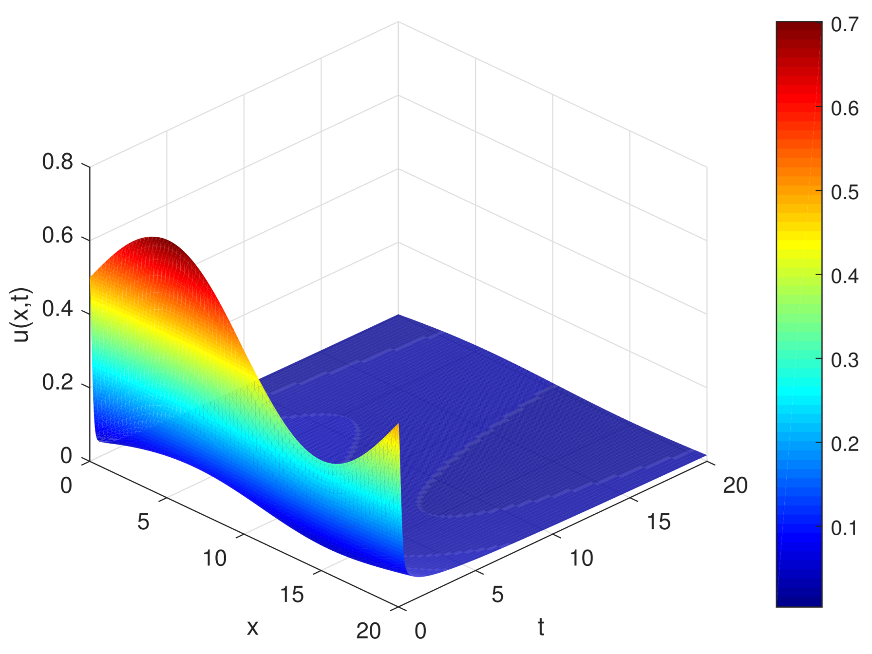
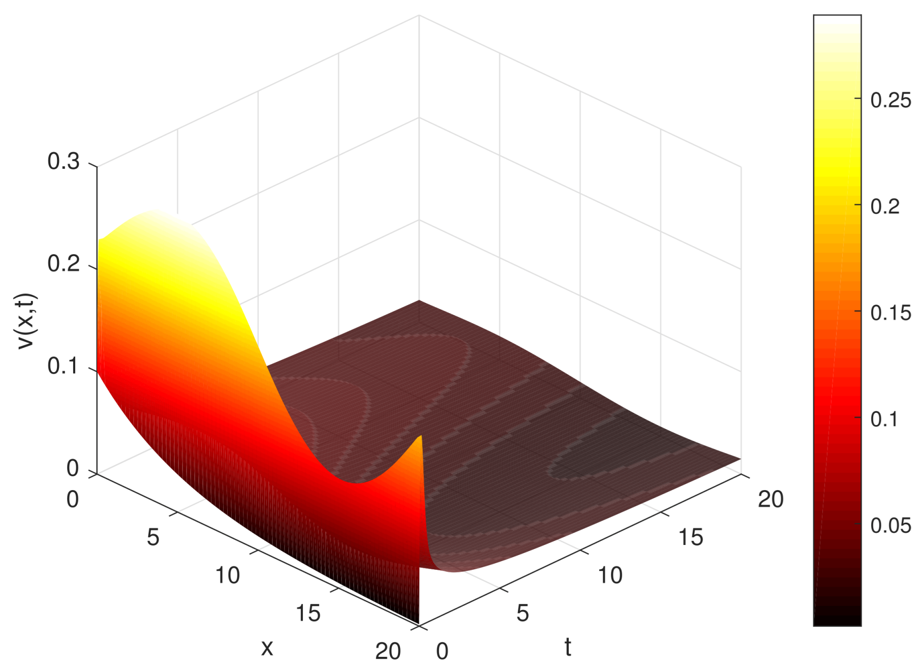
As illustrated in Figure 1 and Figure 2, the variable $u(x,t)$ converges monotonically toward its steady-state value $u^{*}$, while $v(x,t)$ simultaneously decays to $v^{*}$. Throughout the evolution, both profiles remain strictly positive for all x and t, thereby confirming the asymptotic stability of the equilibrium predicted in Theorem 3. It is also observed that the convergence rate decreases as the fractional order ${\vartheta }_1$ becomes smaller, highlighting the subdiffusive nature and pronounced memory effects inherent in the fractional dynamics of the system.

Example 2.

To examine the effect of fractional orders on temporal convergence, we consider the same system (22) with modified parameters:

$$d_1=0.01,d_2=0.03,\beta =0.2,e=0.015,\gamma =0.6.$$

The fractional orders are chosen as

$${\vartheta }_1=0.8,{\vartheta }_2=0.95.$$

The spatial and temporal grids remain identical to those in Example 1. The initial conditions are given by

$$u(x,0)=1.2+0.3sin\left({\displaystyle \frac{\pi x}{L}}\right),v(x,0)=0.2+0.15cos\left({\displaystyle \frac{\pi x}{L}}\right).$$

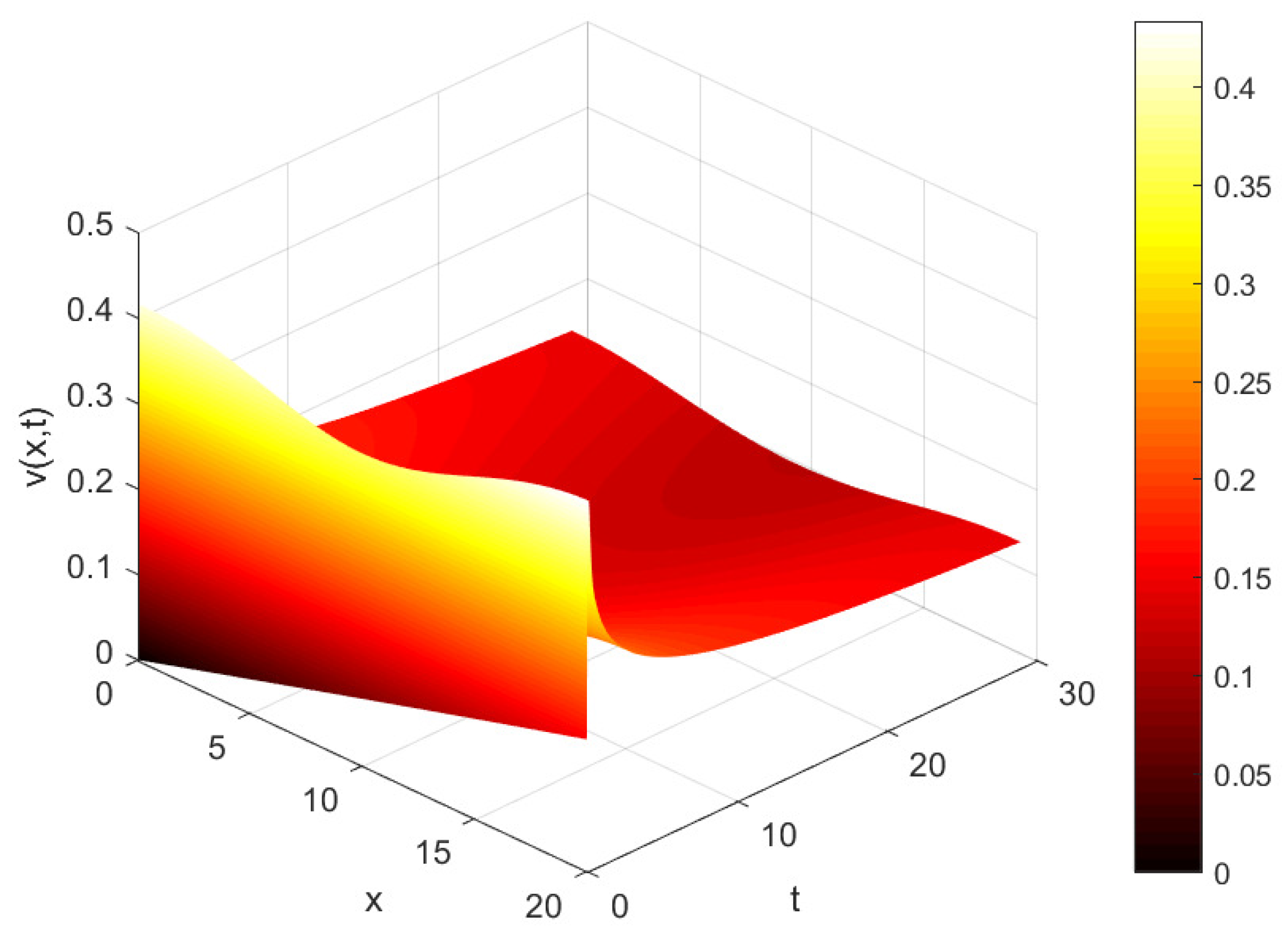
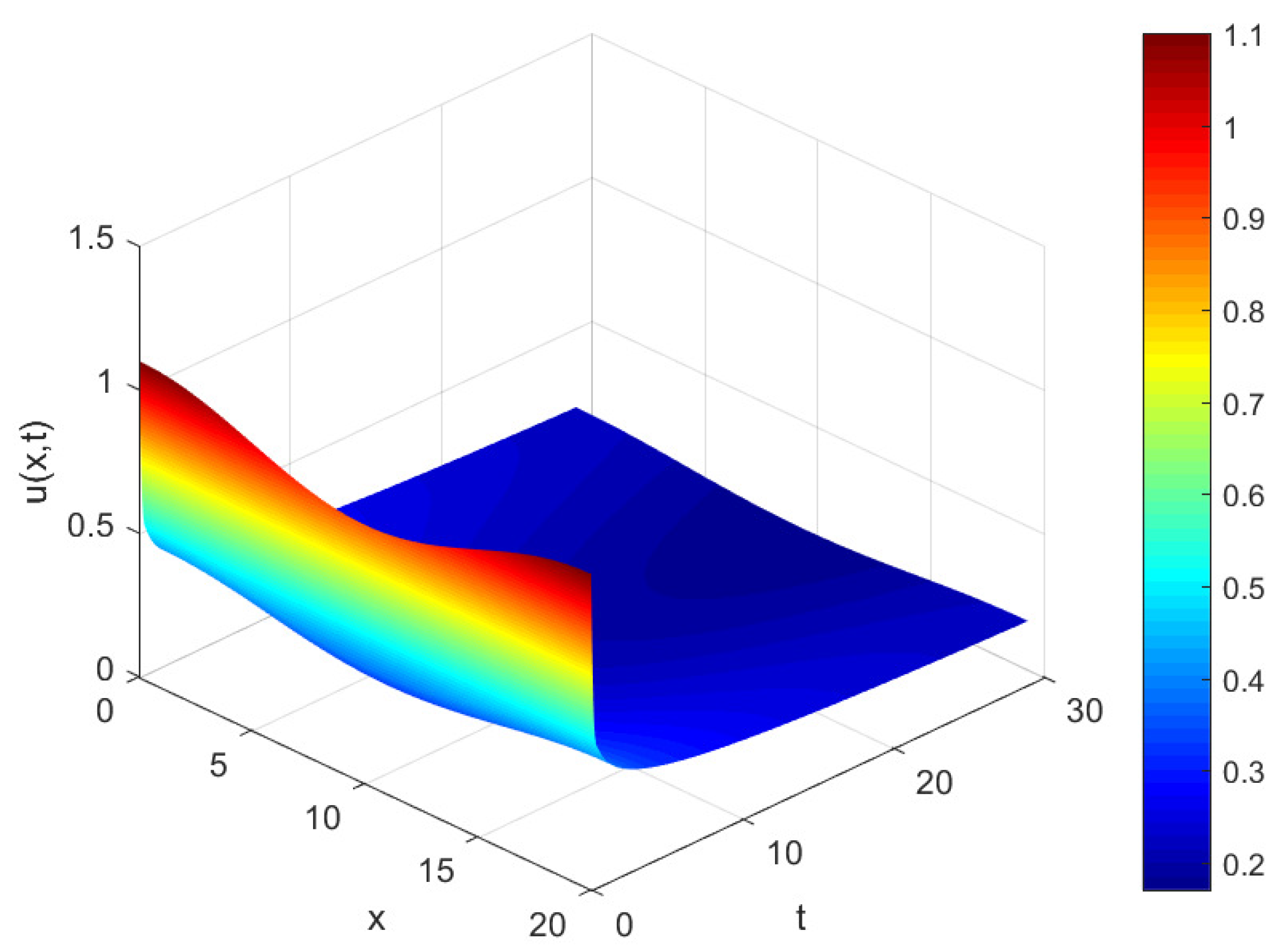
As depicted in Figure 3 and Figure 4, both state variables converge toward the same equilibrium point $(u^{*},v^{*})$ as in the previous example, but with a markedly faster rate. This behavior results from the diminished memory influence as the fractional orders ${\vartheta }_1,{\vartheta }_2\to 1$, which effectively drives the system closer to its classical integer-order dynamics. Higher fractional orders enhance the diffusive effects and attenuate transient oscillations, thereby promoting a quicker stabilization of the system. These numerical findings are in excellent agreement with the theoretical stability analysis presented in Section 4.

The numerical results confirm the analytical stability predictions derived for the incommensurate fractional reaction–diffusion system. In particular, decreasing the fractional orders slows down the return to equilibrium and suppresses the onset of spatial instabilities. The heterogeneous memory exponents produce asymmetric transient patterns consistent with the theoretical spectral criteria. Limitations include the 1D spatial domain and moderate grid resolution; future work may address 2D and 3D extensions.

Several alternative methods exist for solving fractional differential equations, including fractional non-polynomial spline methods, rational spline approaches, logarithmic and hyperbolic spline schemes, and conformable-based numerical techniques. These methods often improve accuracy for smooth solutions or reduce computational cost, but the L1 method remains widely used due to its simplicity and robustness for Caputo derivatives.

6. Conclusions

Compared to previous studies on commensurate fractional FitzHugh–Nagumo systems and incommensurate ODE models, the present work offers the first explicit local stability criteria for an incommensurate fractional reaction–diffusion PDE, bridging a clear gap in the literature. Our analysis extends the results of [X, Y] by incorporating both spatial diffusion and heterogeneous fractional orders, providing a more general framework that can capture the interplay between local kinetics, memory effects, and spatial transport.

In this study, we introduced a novel incommensurate fractional-order FitzHugh–Nagumo reaction–diffusion model and performed a comprehensive local stability analysis. By assigning distinct fractional orders to each state variable, the framework generalizes classical integer-order and commensurate fractional models, offering a versatile description of neuronal excitability and diffusion-driven phenomena.

The derived stability conditions explicitly link equilibrium behavior to fractional orders and diffusion parameters, highlighting how heterogeneity in memory can modulate excitability thresholds, induce bifurcations, and shape transient dynamics. Numerical simulations confirmed that the stability landscape and convergence rates are highly sensitive to the choice of fractional orders, validating the theoretical predictions.

The effectiveness of the proposed approach lies in its analytical transparency and computational efficiency. Unlike previous methods that rely solely on numerical simulations or treat commensurate orders, our formulation provides closed-form stability thresholds that are straightforward to implement and interpret. This enables direct comparisons between different parameter regimes and facilitates the design of control or intervention strategies in excitable media. For large-scale or highly stiff systems, the integration with high-order fractional solvers may further improve efficiency, offering an advantage over conventional integer-order or uniform fractional approaches.

Future research directions include extending the analysis to global stability and bifurcation phenomena, incorporating stochastic perturbations, and exploring random-order or networked extensions. Such developments will further clarify the role of fractional and heterogeneous memory effects in neuronal dynamics, chemical pattern formation, and other interdisciplinary applications.

References

1. Turing, A.M. The chemical basis of morphogenesis. Philos. Trans. R. Soc. B 1952, 237, 37–72. [Google Scholar] [CrossRef]
2. Murray, J.D. Mathematical Biology II: Spatial Models and Biomedical Applications, 3rd ed.; Springer: Cham, Switzerland, 2003. [Google Scholar]
3. Grindrod, P. Patterns and Waves: The Theory and Applications of Reaction–Diffusion Equations; Oxford University Press: Oxford, UK, 1996. [Google Scholar]
4. Tyson, J.J.; Keener, J.P. Singular perturbation theory of traveling waves in excitable media. Phys. D Nonlinear Phenom. 1998, 32, 327–361. [Google Scholar] [CrossRef]
5. Zheng, Q.; Shen, J. Pattern formation in the FitzHugh–Nagumo model. Comput. Math. Appl. 2015, 70, 1082–1097. [Google Scholar] [CrossRef]
6. Casten, R.G.; Holl, C.J. Stability properties of solutions to systems of reaction-diffusion equations. SIAM J. Appl. Math. 1977, 33, 353–364. [Google Scholar] [CrossRef]
7. Tasbozan, O. A popular reaction-diffusion model fractional Fitzhugh-Nagumo equation: Analytical and numerical treatment. Appl. Math. J. Chin. Univ. 2021, 36, 218–228. [Google Scholar] [CrossRef]
8. Ringqvist, M. On dynamical behaviour of FitzHugh-Nagumo systems. Res. Rep. Math. 2006, 5, 1–81. [Google Scholar] [CrossRef]
9. FitzHugh, R. Impulses and physiological states in theoretical models of nerve membrane. Biophys. J. 1961, 1, 445–466. [Google Scholar] [CrossRef]
10. Nagumo, J.; Arimoto, S.; Yoshizawa, S. An active pulse transmission line simulating nerve axon. Proc. IRE 1962, 50, 2061–2070. [Google Scholar] [CrossRef]
11. Hodgkin, A.L.; Huxley, A.F. A quantitative description of membrane current and its application to conduction and excitation in nerve. J. Physiol. 1952, 117, 500–544. [Google Scholar] [CrossRef]
12. Alimova, N.B. Mathematical Modeling of the Neuron Autocoling in the Cell Membrane Using the Fractional Model of FitzHugh-Nagumo with the Function of Irritant Intensity. Bulletin KRASEC. Phys. Math. Sci. 2024, 48, 56–69. [Google Scholar]
13. Ghafoor, A.; Fiaz, M.; Hussain, M.; Ullah, A.; Ismail, E.A.; Awwad, F.A. Dynamics of the time-fractional reaction–diffusion coupled equations in biological and chemical processes. Sci. Rep. 2024, 14, 7549. [Google Scholar] [CrossRef] [PubMed]
14. Owolabi, K.M.; Jain, S.; Pindza, E.; Mare, E. Comprehensive Numerical Analysis of Time-Fractional Reaction–Diffusion Models with Applications to Chemical and Biological Phenomena. Mathematics 2024, 12, 3251. [Google Scholar] [CrossRef]
15. Merga, F.E.; Duressa, G.F. Exponential B-spline collocation method for singularly perturbed time-fractional delay parabolic reaction-diffusion equations. J. Numer. Anal. Approx. Theory 2024, 53, 279–297. [Google Scholar] [CrossRef]
16. Podlubny, I. Fractional Differential Equations; Academic Press: Cambridge, MA, USA, 1999. [Google Scholar]
17. Mainardi, F. Fractional Calculus and Waves in Linear Viscoelasticity; Imperial College Press: London, UK, 2010. [Google Scholar]
18. Metzler, R.; Klafter, J. The random walk’s guide to anomalous diffusion: A fractional dynamics approach. Phys. Rep. 2000, 339, 1–77. [Google Scholar] [CrossRef]
19. Tarasov, V.E. Fractional Dynamics: Applications of Fractional Calculus to Dynamics of Particles, Fields and Media; Springer: Cham, Switzerland, 2011. [Google Scholar]
20. Magin, R.L. Fractional Calculus in Bioengineering; Begell House: Danbury, CT, USA, 2006. [Google Scholar]
21. Hammad, M.M.A.; Bendib, I.; Alshanti, W.G.; Alshanty, A.; Ouannas, A.; Hioual, A.; Momani, S. Fractional-order Degn–Harrison reaction–diffusion model: Finite-time dynamics of stability and synchronization. Computation 2024, 12, 144. [Google Scholar] [CrossRef]
22. Petras, I. Fractional-Order Nonlinear Systems: Modeling, Analysis and Simulation; Springer Science & Business Media: Berlin/Heidelberg, Germany, 2011. [Google Scholar]
23. Momani, S.; Djenina, N.; Ouannas, A.; Batiha, I.M. Stability Results for Nonlinear Fractional Differential Equations with Incommensurate Orders. IFAC-PapersOnLine 2024, 58, 286–290. [Google Scholar] [CrossRef]
24. Henry, B.I.; Langlands, T.A.M.; Wearne, S.L. Anomalous diffusion with linear reaction dynamics: From continuous time random walks to fractional reaction–diffusion equations. Phys. Rev. E 2006, 74, 031116. [Google Scholar] [CrossRef]
25. Liu, F.; Zhuang, P.; Turner, I.; Anh, V.; Burrage, K. A semi-alternating direction method for a 2-D fractional FitzHugh–Nagumo monodomain model on an approximate irregular domain. J. Comput. Phys. 2015, 293, 252–263. [Google Scholar] [CrossRef]
26. Chen, W. Time–space fabric underlying anomalous diffusion. Chaos Solitons Fractals 2006, 28, 923–929. [Google Scholar] [CrossRef]
27. Diethelm, K.; Ford, N.J. The analysis of fractional differential equations. In Lecture Notes in Mathematics, 2004; Springer: Berlin/Heidelberg, Germany, 2010. [Google Scholar]
28. Brandibur, O.; Kaslik, E. Stability analysis for a fractional-order coupled FitzHugh–Nagumo-type neuronal model. Fractal Fract. 2022, 6, 257. [Google Scholar] [CrossRef]
29. Almusawa, M.Y.; Aldawsari, K.; Mshary, N. Exploring fractional dynamics in the FitzHugh-Nagumo model with the Caputo operator. Bound. Value Probl. 2025, 2025, 127. [Google Scholar] [CrossRef]
30. Alidousti, J.; Ghaziani, R.K. Spiking and bursting of a fractional order of the modified FitzHugh-Nagumo neuron model. Math. Model. Comput. Simulations 2017, 9, 390–403. [Google Scholar] [CrossRef]
31. Gao, D. Random dynamics of fractional stochastic retarded FitzHugh–Nagumo systems on unbounded domains. J. Inequalities Appl. 2025, 2025, 76. [Google Scholar] [CrossRef]
32. Bendib, I.; Ouannas, A.; Al Horani, M.; Dalah, M. Dynamics in finite time of the fractional-order FitzHugh–Nagumo model: Stability, synchronization, and simulations. In Fractional Calculus and Applications (ICFCA 2024, Springer Proceedings in Mathematics & Statistics); Naifar, O., Ben Makhlouf, A., Hammami, M.A., Eds.; Springer: Cham, Switzerland, 2025; Volume 505. [Google Scholar] [CrossRef]
33. Chen, L.; Xue, M.; Lopes, A.; Wu, R.; Chen, Y. Asymptotic behavior of fractional-order nonlinear systems with two different derivatives. J. Eng. Math. 2023, 140, 9. [Google Scholar] [CrossRef]
34. Brandibur, O.; Kaslik, E. Stability of two-component incommensurate fractional-order systems and applications to the investigation of a FitzHugh–Nagumo neuronal model. Math. Methods Appl. Sci. 2018, 41, 7182–7194. [Google Scholar] [CrossRef]
35. Wang, X.; Wang, Z.; Dang, S. Dynamic behavior and fixed-time synchronization control of incommensurate fractional-order chaotic system. Fractal Fract. 2024, 9, 18. [Google Scholar] [CrossRef]
36. Wu, Z.; Wang, Z.; Cai, Y.; Yin, H.; Wang, W. Pattern formation in a fractional-order reaction-diffusion predator-prey model with Holling-III functional response. Adv. Contin. Discret. Model. 2025, 2025, 29. [Google Scholar] [CrossRef]
37. Lin, Y.; Xu, C. Finite difference/spectral approximations for the time-fractional diffusion equation. J. Comput. Phys. 2007, 225, 1533–1552. [Google Scholar] [CrossRef]
Figure 1. Spatio-temporal evolution of u ( x , t ) for Example 1 with ϑ 1 = 0.7 ,   ϑ 2 = 0.9 . The solution converges smoothly toward the positive equilibrium.
Symmetry 18 00052 g001
Figure 2. Evolution of v ( x , t ) for Example 1 showing asymptotic decay toward v * . Fractional memory produces a smooth, monotonic convergence.
Symmetry 18 00052 g002
Figure 3. Surface plot of u ( x , t ) for Example 2. Higher fractional orders yield faster convergence to equilibrium.
Symmetry 18 00052 g003
Figure 4. Temporal evolution of v ( x , t ) for Example 2. The system stabilizes rapidly as memory effects diminish.
Symmetry 18 00052 g004
Disclaimer/Publisher’s Note: The statements, opinions and data contained in all publications are solely those of the individual author(s) and contributor(s) and not of MDPI and/or the editor(s). MDPI and/or the editor(s) disclaim responsibility for any injury to people or property resulting from any ideas, methods, instructions or products referred to in the content.