Symmetry-Guided Analysis of Market Characteristics and Electricity Prices Anomaly: A Comparative Framework of Influencing Factors

Abstract

Electricity spot prices jointly encode network physics and strategic bidding outcomes. In a well-functioning market, nodal and temporal price patterns tend to remain approximately invariant under mild perturbations-exhibiting symmetry-preserving regularities in distribution shape, spatial gradients, and temporal variation. Conversely, congestion binding, net-load stress, and abnormal bidding can induce symmetry breaking, manifested as heavy tails, mean shifts, and localized price discontinuities. This study develops a symmetry-guided and explainable diagnostic framework to identify price anomalies and attribute their dominant drivers. First, representative anomaly types (spike and mean shift) are defined using statistically and operationally motivated criteria, together with robustness checks across alternative thresholds. Second, principal component analysis is applied to construct compact, anomaly-specific feature sets, filtering weakly related variables while retaining system stress, congestion proxies, and renewable-induced variability indicators. Third, leveraging the optimization structure of market clearing and the associated KKT conditions, we characterize the price–feature linkage as a piecewise mapping and quantify each feature’s contribution via a sampling-based influence scoring procedure, yielding a ranked causal attribution. Case studies on a regional day-ahead spot market dataset demonstrate that the proposed framework achieves high consistency with expert assessments, with traceability accuracy exceeding 85% overall and particularly strong performance for spike-type anomalies. The method reduces reliance on purely manual diagnosis and black-box learning, and provides symmetry-oriented, actionable evidence for market surveillance and renewable-friendly flexibility and congestion management design. The proposed framework enables transparent identification of dominant structural drivers underlying different types of electricity price anomalies, linking observed price signals to market-clearing mechanisms. The results provide actionable diagnostic insights for market monitoring and regulatory assessment in electricity markets with high renewable penetration.

1. Introduction

The development of electricity markets has been recognized as essential for optimizing the allocation of power resources and enhancing overall system efficiency [1,2]. Under profound changes in the global energy landscape, electricity market reforms have been successively implemented by major economies to improve market adaptability and operational flexibility [3,4]. In these reforms, electricity pricing has been positioned as the primary mechanism through which resource allocation is directed and economic signals are conveyed. As a price-driven market, electricity prices have been regarded as carriers of both the commodity attributes and the market value of electricity. However, electricity prices have been jointly shaped by market supply [5], load demand [6], market structure [7], competitive dynamics [8], and regulatory policies [9]. When these factors fluctuate, pronounced price volatility or even anomalous price behavior has been induced, and market stability and credibility have been undermined accordingly [10]. When severe fluctuations persist, operational and financial risks are amplified, market participation is discouraged, and overall market efficiency is eroded [11]. Among the contributing factors, irregular pricing has been induced by anomalous bidding strategies of power producers or deficiencies in market regulation, so that the economic signals embedded in prices have been distorted and inefficient resource allocation has been triggered [12,13]. In extreme cases, market efficiency has not only been impaired, but risks to the secure and stable operation of power systems have also been posed [14]. From a symmetry perspective, understood here as a structure-based analytical viewpoint, such phenomena can be interpreted as symmetry-breaking, where approximate symmetry in price distributions has been disrupted and asymmetric deviations across nodes or timeframes have been amplified. It should be emphasized that the present study does not aim to develop a new generic anomaly detection algorithm but rather focuses on a symmetry-guided analytical framework for interpreting and attributing electricity price anomalies under market-clearing mechanisms. Therefore, a systematic analysis of the root causes behind electricity price anomalies has been required. By establishing traceable links between price signals and their underlying drivers, distortions in the market-clearing process can be identified and corrected, thereby supporting well-functioning electricity markets and more efficient and reliable market structures [15].

In recent years, the large-scale integration of variable renewable energy (VRE) resources, such as wind and photovoltaic generation, has been regarded as a key driver that reshapes electricity market operations [16]. Due to intermittency and forecast uncertainty, fluctuations in net load and network power flows have been intensified, and symmetry-breaking conditions in both temporal and spatial price patterns have been more frequently induced [17]. Under episodes of extreme renewable output, steep ramping events, and concentrated curtailment, short-term price spikes or persistent mean shifts have been triggered, and the price signals used for investment decisions and operational strategies have been distorted accordingly [18]. In this context, the identification and tracing of symmetry-breaking price anomalies have been deemed essential for market-rule refinement and regulatory interventions that support large-scale renewable accommodation [19]. Moreover, a symmetry-guided diagnostic viewpoint has been required to distinguish symmetry-preserving price variability, which reflects efficient renewable utilization and rational market responses, from symmetry-breaking anomaly patterns that indicate structural bottlenecks, insufficient system flexibility, or misaligned bidding behavior. Such a distinction naturally motivates a diagnostic framework that goes beyond anomaly identification and instead emphasizes structure-aware interpretation of different anomaly types.

Research has been conducted on the drivers of electricity price anomalies. The existing studies have been broadly categorized into factor-specific and multi-factor analytical approaches. In factor-specific approaches, the effect of a single class of variables has been emphasized. For example, clustering methods have been applied to investigate relationships between electricity prices and load characteristics, where load has been treated as the dominant determinant [20,21]. In multi-factor approaches, multiple influencing factors have been jointly considered, and tools such as correlation and regression analysis, graphical modeling, or principal component analysis (PCA) have been adopted to reveal direct and indirect impacts of demand, generation structure, and other market variables on prices [22,23]. Although useful insights have been provided into the role of individual and combined factors, underlying symmetry-preserving structures in price formation and the symmetry-breaking perturbations that drive deviations from normal patterns have seldom been explicitly characterized. When such symmetry structures are made explicit, interpretability can be improved and diagnostic results can be more coherently organized, which is critical for market surveillance and regulatory assessment. However, most existing studies remain primarily focused on identifying influential factors or statistical correlations, rather than establishing a symmetry-guided attribution framework that explicitly links anomaly patterns to structural conditions in the market-clearing process.

From the perspective of anomaly tracing, a reliable correspondence between electricity price signals and their underlying influencing factors has been required, and dominant drivers of different anomaly types have been inferred accordingly. In recent developments, data-driven and machine learning techniques have been leveraged to identify or forecast price spikes and abnormal fluctuations in markets with high renewable penetration [24,25]. Strong predictive capabilities have been demonstrated, but heavy reliance on large volumes of historical data have typically been imposed, and black-box behavior has often been exhibited, so causal diagnosis has been limited, especially under data-scarce settings. In parallel, economic modeling frameworks, such as security-constrained unit commitment and security-constrained economic dispatch, have been adopted to represent market-clearing processes and physical constraints in a structured manner [26,27]. However, due to the high dimensionality and complexity of modern electricity markets, comprehensive and efficient characterization of multi-faceted drivers and emergent nonlinear interactions has remained difficult when purely model-based analysis is used. Typical examples include recurrent neural networks such as LSTM, autoencoder-based anomaly detection models, and graph neural networks that exploit spatial correlations in nodal prices. While these approaches are effective for pattern recognition and prediction, they do not explicitly embed market-clearing constraints or economic rationality conditions, which limits their suitability for diagnostic attribution and regulatory analysis.

To address these limitations, a symmetry-guided perspective has been adopted, where normal market operations are characterized as symmetry-preserving, and electricity price anomalies are interpreted as symmetry-breaking events, serving as the basis for structure-aware anomaly attribution rather than anomaly detection. Thus, a hybrid diagnostic framework has been constructed by integrating the structural economic logic and market-clearing constraints with data-driven feature extraction (e.g., PCA) and structured influence scoring. Compared with purely black-box machine learning models, interpretability and causal attribution have been emphasized, while greater flexibility and scalability than traditional economic models have been maintained for handling high-dimensional disturbances and limited-data conditions. The proposed framework is evaluated primarily in terms of attribution consistency, interpretability, and robustness, rather than predictive or detection accuracy, which distinguishes it from conventional baseline models. Through this symmetry-oriented hybrid framework, actionable evidence for tracing the causes of electricity price anomalies can be provided, and support can be offered for market surveillance, regulatory assessment, and resilient system design. The conclusions drawn in this study are methodological and mechanism-oriented, with empirical data serving to validate the robustness of the proposed attribution logic rather than to establish purely statistical generalization.

2. Electricity Spot Market Price Signal Generation and Symmetry—Based Assessment

Under the day-ahead market-clearing framework, generators participate by submitting supply offers in the form of price–quantity bid pairs, whereas demand-side participants submit quantity-only bids that specify expected consumption profiles without explicit price offers. The day-ahead electricity market operates under a full-energy bidding mechanism with centralized, optimization-based clearing. For each operating day, market participants report unit commitment plans, generation schedules, and associated offer prices, while renewable energy trading units additionally submit short-term power output forecasts to account for the variability and uncertainty of wind and photovoltaic generation. The power dispatching authority aggregates the submitted information and incorporates load forecasts, interregional transmission and reception schedules, non-market unit generation plans, generator maintenance arrangements, operational constraints of generating units, and grid security constraints into a unified market-clearing model. The clearing process is formulated with the objective of maximizing social welfare, thereby determining the optimal time-coupled generation dispatch trajectory and the corresponding locational marginal prices (LMPs) for the operating day. The price formation is governed by an LMP-based pricing mechanism, the mathematical formulation of which is presented below.

2.1. Price Signal Generation in Spot Market Clearing

2.1.1. Objective Function

The nodal electricity price calculation model minimizes the overall system operating cost through optimization, and the objective function is:

$$\min \sum _{\mathit{i}=1}^{{\mathit{N}}^{\mathit{G}}}\sum _{\mathit{t}=1}^{\mathit{T}}\left({\mathit{c}}_{\mathit{i},\mathit{t}}{\mathit{P}}_{\mathit{i},\mathit{t}}\right)+\sum _{\mathit{l}=1}^{{\mathit{N}}^{\mathrm{L}}}\sum _{\mathit{t}=1}^{\mathit{T}}{\mathit{M}}^{\mathrm{pen}}({\mathit{L}}_{\mathit{l},\mathit{t}}^{+}+{\mathit{L}}_{\mathit{l},\mathit{t}}^{-}) ,$$

(1)

where ${\mathit{N}}^{\mathit{G}}$ and ${\mathit{N}}^{\mathrm{L}}$ denote the total numbers of market units and transmission branches, respectively, and t is the number of time slots in the day-ahead clearing horizon. ${\mathit{c}}_{\mathit{i},\mathit{t}}$ and ${\mathit{P}}_{\mathit{i},\mathit{t}}$ represent the offer price and scheduled output of market unit I and time t. ${\mathit{M}}^{\mathit{pen}}$ is the penalty coefficient associated with line-flow constraint relaxation, while ${\mathit{L}}_{\mathit{l},\mathit{t}}^{+}$ and ${\mathit{L}}_{\mathit{l},\mathit{t}}^{-}$ are the positive and negative power-flow slack variables of branch l. The optimization explicitly targets market-based units whose bids include both price and quantity; outputs of non-market units, determined by administrative dispatch, enter the load-balance constraints as fixed parameters, ensuring that their contribution is reflected in the clearing process.

2.1.2. System Load Balance Constraints

The system load balance equation is revised to include both market and non-market generation outputs. Let $M$ denote the set of market units and $N$ represent that of non-market units. Then, the balance constraint at node $\mathit{j}$ and time t becomes:

$$\sum _{i\in \mathrm{M}}{P}_{i,t}+\sum _{i\in \mathrm{N}}{\overline{P}}_{k,t}=D_{j,t},$$

(2)

where ${\overline{P}}_{k,t}$ is the scheduled (fixed) output of non-market unit $k$ at time $t$. The fixed values are typically determined through administrative dispatch and are treated as constants during market clearing.

2.1.3. Upper and Lower Unit Output Constraints

$${\mathit{P}}_{\mathit{i},\mathit{t}}^{\min }{\mathrm{u}}_{\mathit{i},\mathit{t}}\le {\mathit{P}}_{\mathit{i},\mathit{t}}\le {\mathit{P}}_{\mathrm{i},\mathrm{t}}^{\max }{\mathit{u}}_{\mathit{i},\mathit{t}} \forall \mathit{i}\in {\mathit{N}}^{\mathrm{G}},\forall \mathit{t}\in \mathrm{T}$$

(3)

In Equation (3), ${\mathit{P}}_{\mathit{i},\mathit{t}}^{\mathit{min}}$ and ${\mathit{P}}_{\mathit{i},\mathit{t}}^{\mathit{min}}$ are the upper and lower limits of the rated output of market unit i at time period t, respectively; ${\mathit{u}}_{\mathit{i},\mathit{t}}$ characterizes the start–stop status of market unit i at time period t, which is 0 if it is stopped and 1 otherwise.

2.1.4. Unit Ramping Constraints

In power system operations, the output adjustment of generating units must comply with specific ramping rate limits to ensure equipment safety and grid stability. The constraints are defined as (4) and (5):

$$\left\{\begin{array}{l}{P}_{i,t}-P_{i,t-1}\le \Delta P_i^{\mathrm{U}} \forall i\in N^{\mathrm{G}},\forall t=2,\dots ,T\\ P_{i,1}-P_{i,0}\le \Delta P_i^{\mathrm{U}} \forall i\in N^{\mathrm{G}}\end{array}\right.$$

(4)

$$\left\{\begin{array}{l}{P}_{i,t}-P_{i,t-1}\ge -\Delta P_i^{\mathrm{D}} \forall i\in N^{\mathrm{G}},\forall t=2,\dots ,T\\ P_{i,1}-P_{i,0}\ge -\Delta P_i^{\mathrm{D}} \forall i\in N^{\mathrm{G}}\end{array}\right.,$$

(5)

where $\mathit{\Delta }{\mathit{P}}_{\mathit{i}}^{\mathrm{U}}$ and $\mathit{\Delta }{\mathit{P}}_{\mathit{i}}^{\mathrm{D}}$ denote the maximum ramp-up rate and maximum ramp-down rate of market unit i, respectively.

2.1.5. Branch Power Flow Constraints

$${-\mathrm{P}}_{\mathit{l}}^{\max }\le \sum _{i=1}^{N^{\mathrm{G}}}{G}_{l-i}{P}_{i,t}+\sum _{k=1}^{N^{\mathrm{B}}}{\mathit{G}}_{\mathit{l}-\mathit{k}}{D}_{k,t}-L_{l,t}^{+}+L_{l,t}^{-}\le {\mathit{P}}_{\mathit{l}}^{\max } \forall l\in N^{\mathrm{L}}$$

(6)

In (6), ${\mathit{P}}_{\mathit{l}}^{\mathit{max}}$ denotes the power flow transmission limit of branch l; ${\mathit{N}}^{\mathit{L}}$ denotes the total number of branches in the system; ${\mathit{G}}_{\mathit{l}-\mathit{i}}$ denotes the power transfer distribution factor where market unit i is located to transmission line l; ${\mathit{G}}_{\mathit{l}-\mathit{k}}$ denotes the power transfer distribution factor of node k to line l.

2.1.6. Locational Marginal Price Calculation

After solving the above day-ahead electricity energy market-clearing model, the pairwise multipliers of the system load balance constraints and branch power flow constraints for each time period can be obtained, and then the price of node i at time period t can be given by Equation (7):

$${\mathit{\lambda }}_{\mathit{k},\mathit{t}}={\mathit{\mu }}_{\mathit{t}}\sum _{l=1}^{N^{\mathrm{L}}}\left({\mathit{\sigma }}_{\mathit{l},\mathit{t}}^{\max }-{\mathit{\sigma }}_{\mathit{l},\mathit{t}}^{\min }\right)G_{l-k}$$

(7)

where ${\mathit{\lambda }}_{\mathit{k},\mathit{t}}$ denotes the price of node k at time period t; ${\mathit{\mu }}_{\mathit{t}}$ denotes the dual multiplier of the system load balance constraint at time period t; ${\mathit{\sigma }}_{\mathit{l},\mathit{t}}^{\mathit{max}}$ and ${\mathit{\sigma }}_{\mathit{l},\mathit{t}}^{\mathit{min}}$ denote the dyadic multipliers of the maximum forward and reverse power flow constraints of branch l, respectively. According to Equation (6), it can be shown that when the branch power flow constraint is over the limit, which means the variables ${\mathit{L}}_{\mathit{l},\mathit{t}}^{+}$ and ${\mathit{L}}_{\mathit{l},\mathit{t}}^{-}$ are not zero, the ${\mathit{\sigma }}_{\mathit{l},\mathit{t}}^{\mathit{max}}$ and ${\mathit{\sigma }}_{\mathit{l},\mathit{t}}^{\mathit{min}}$ are the relaxation penalty factor for network power flow constraints, which is set by the power dispatch center. Here, these penalty multipliers correspond to the dual variables (shadow prices) associated with binding network power flow constraints in the market-clearing optimization, reflecting the marginal economic cost of congestion or scarcity rather than an exogenous penalty term.

Although the price formation mechanism has been well structured by market clearing, the resulting price patterns have not always remained stable. Therefore, the notion of symmetry has been introduced to distinguish symmetry-preserving regularities from symmetry-breaking deviations.

2.2. Symmetry-Preserving Regularities and Symmetry-Breaking Deviations

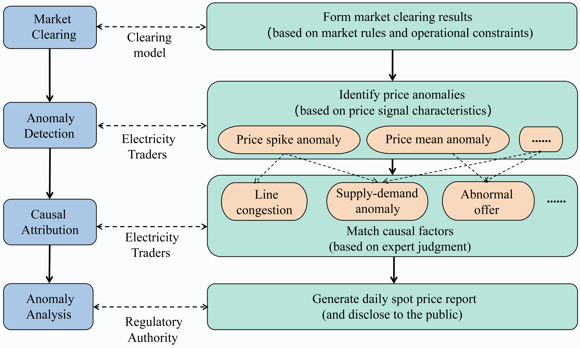
In successfully operating electricity markets, the analysis and assessment of abnormal spot prices are still primarily conducted based on expert judgment and manual experience, as illustrated in Figure 1. The process begins with the market operator determining the market-clearing results, including nodal prices and unit dispatch, using a market-clearing model that accounts for market rules and operational constraints. Based on these results, market participants monitor and classify price anomalies according to price characteristics. Subsequently, experienced analysts identify the underlying causes of price anomalies through expert-driven assessments. Finally, the market regulatory authority compiles and publishes a daily electricity spot market report to enhance market transparency and support the ongoing development of a well-functioning electricity spot market.

An examination of nodal pricing in a regional electricity spot market reveals that price anomalies occur with notable frequency, accounting for nearly 18% of total trading days over a one-year period [28]. These irregularities stem from the complex interplay of multiple price-influencing factors. Currently, anomaly diagnosis relies heavily on manual assessment, which often leads to incomplete or imprecise causal attribution. Additionally, the process tends to be inefficient, requiring significant time and resources to reach conclusions.

2.3. Assessment of Price Anomalies Under a Symmetry-Guided View

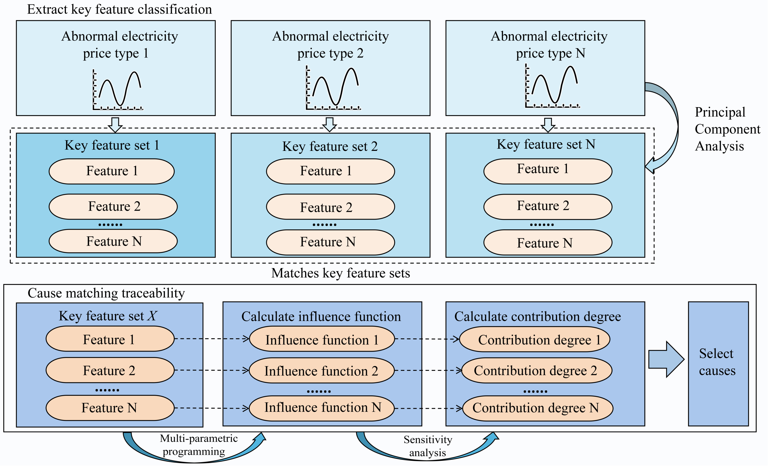
To address the issues above, this paper first performs anomaly price signal classification and feature extraction, followed by causal attribution through a two-step process for analyzing the causes of price anomalies. Here, the term “causal attribution” is used in a mechanism-oriented and diagnostic sense, referring to structure-consistent driver attribution implied by the market-clearing process rather than interventional or econometric causal identification. In this study, symmetry does not refer to a statistical invariance of price series, but to the structural consistency of price–feature relationships implied by the market-clearing mechanism. The detailed methodology is illustrated in Figure 2; it provides the canonical description of the overall framework; subsequent sections focus on implementation details and the empirical instantiation rather than reiterating the full workflow. Initially, based on the historical dataset, a classification of price anomalies is constructed, and principal component analysis (PCA) is employed to extract key feature sets for each signal category. This step ensures that only highly relevant features are considered during the causal attribution process, thus avoiding analysis of low-correlation features. Next, the price anomalies are categorized based on their features, and the corresponding key feature sets are matched. Subsequently, the influence functions are calculated, and the contribution of each feature to the anomaly is assessed. Finally, causal attribution is performed based on the relative contribution of each feature. The details of these two steps are discussed in Section 3 and Section 4.

2.4. Comparison with Black-Box Machine Learning-Based Anomaly Detection Methods

To further clarify the methodological positioning of the proposed framework, a conceptual comparison with representative black-box machine learning-based anomaly detection approaches is summarized in

Table 1. Conceptual comparison between the proposed symmetry-aware framework and black-box ML-based anomaly detection methods.

Aspect	Black-Box ML Methods (LSTM, AE, GNN)	Proposed Symmetry-Aware+ECR-Guided Framework
Primary objective	Anomaly detection/prediction	Diagnostic attribution of anomaly drivers
Model transparency	Low (black-box)	High (structure-consistent, explainable)
Use of market-clearing constraints	Not embedded	Explicitly embedded via optimization structure
Output	Anomaly score/label	Ranked dominant drivers
Data requirement	Large-scale historical data	Moderate data, robust under limited samples
Regulatory interpretability	Limited	High
Role in market monitoring	Early warning	Post-event diagnosis and policy support

. Unlike data-driven models such as LSTM, autoencoder-based methods, or graph neural networks, which primarily focus on anomaly detection or prediction accuracy, the proposed symmetry-aware and ECR-guided framework is designed for diagnostic attribution under market-clearing constraints. The comparison highlights fundamental differences in objectives, transparency, data requirements, and regulatory interpretability, emphasizing that the proposed approach complements rather than replaces the existing black-box methods. This distinction provides important context for the subsequent case studies, where the framework’s diagnostic capability and interpretability are examined through real market data.

2.5. Theoretical Basis for Symmetry in Electricity Market Signals

Electricity prices in well-functioning markets often exhibit structured regularities arising from the interaction of physical constraints and rational bidding behaviors. Under ideal conditions—such as stable supply–demand balance, rational bidding, and uncongested network flows—nodal prices tend to reflect symmetric behavior in both spatial and temporal dimensions. This symmetry is observable through the following aspects:

(1)

Temporal symmetry: Price trajectories over time may exhibit stationarity or periodicity, where prices return to a mean or follow repeating patterns.

(2)

Spatial symmetry: Nodal prices across locations with similar network positions or generation profiles tend to converge or fluctuate within bounded deviations.

(3)

Statistical symmetry: The distribution of price signals across nodes or time steps follows nearly symmetric probability distributions under normal conditions.

In this study, such statistical symmetry measures are used solely for descriptive characterization; the core notion of symmetry is economic and structural, referring to the consistency of price–feature relationships implied by the market-clearing mechanism rather than statistical invariance alone.

Mathematically, this can be expressed using symmetry in the probability density function (PDF) of price-related features. Let $f\left(x\right)$ denote the PDF of a feature such as nodal price deviation or ramp change rate. Symmetric behavior implies as:

$$P_t^{sym}=f\left(x\right)\approx \mathit{f}(-\mathit{x}),$$

(8)

where $x$ is the deviation from the mean or expected value. Deviations from this symmetry indicate anomaly-prone behavior, often associated with network congestion, market power, or renewable forecast errors.

Furthermore, this statistical symmetry can be characterized by zero skewness (as shown in Equation (9) and stable covariance structures, as shown in Equation (10).

$$Skew(P_t)={\displaystyle \frac{E\left[{{(P}_t-\mu )}^3\right]}{{\sigma }^3}}\approx 0$$

(9)

$$\Sigma =Cox\left(X\right) \mathit{where} X \mathit{is\; the\; feature\; vector}$$

(10)

Asymmetric conditions lead to heavy tails, mean shifts, or spike-like deviations in price signals. These can be interpreted as symmetry-breaking phenomena, whose detection forms the foundation of our anomaly identification framework.

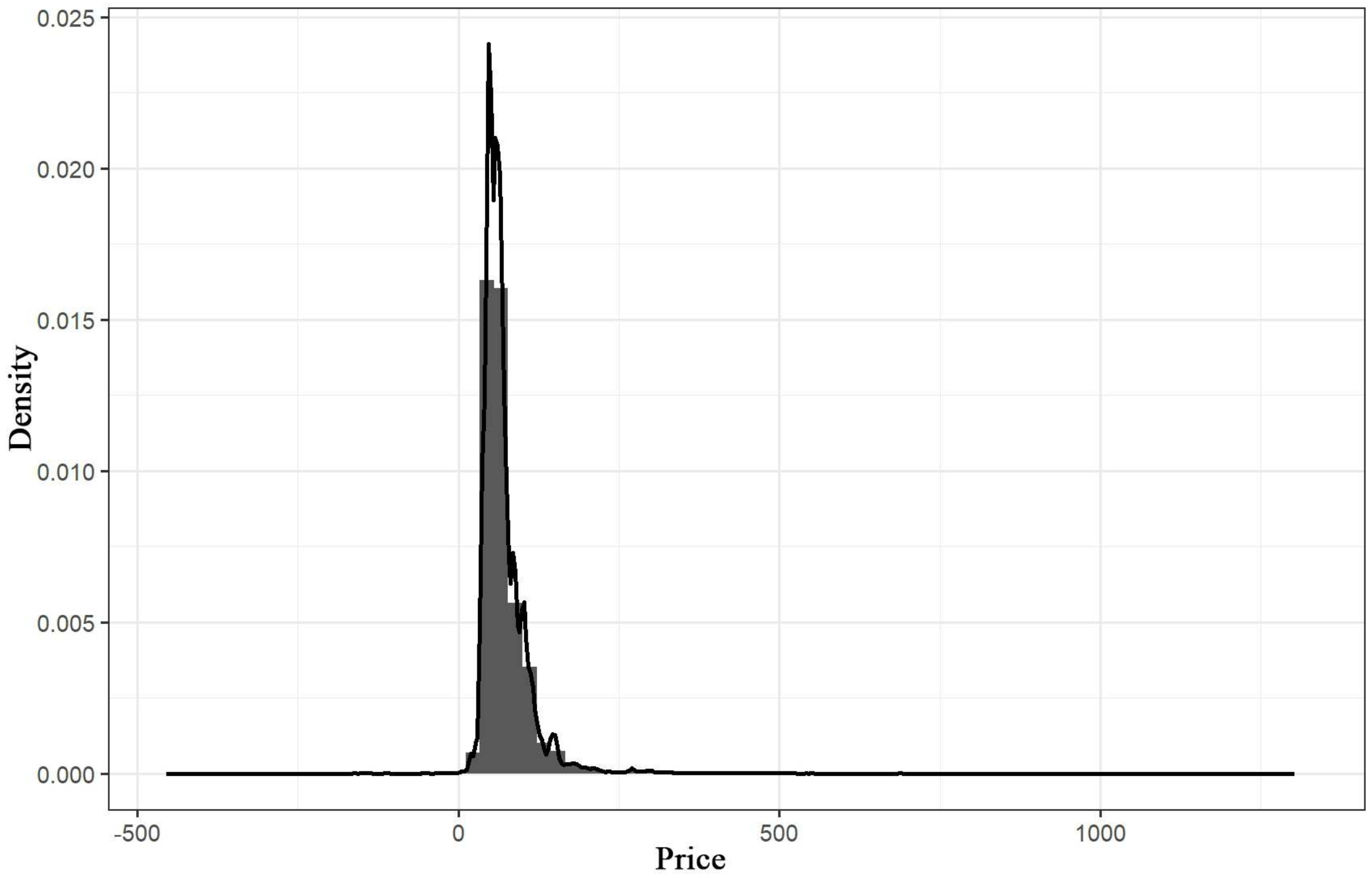
Figure 3 illustrates the histogram of electricity prices over the study period. The distribution exhibits a pronounced right-skewed pattern (skewness = 4.3), with the majority of observations concentrated at relatively low price levels and a long right tail corresponding to extreme price realizations. This asymmetric distribution indicates that price spikes occur infrequently but with large magnitudes, which is consistent with symmetry-breaking behavior induced by localized congestion, scarcity, or extreme operating conditions rather than normal market variability.

In summary, spot price signals have been generated through market clearing, and anomaly patterns have been assessed under a symmetry-guided interpretation. However, the dominant drivers behind different symmetry-breaking anomalies have not been directly observable from prices alone. These drivers should be interpreted as structurally dominant factors associated with price anomalies rather than as variables exerting independently identified causal effects. Therefore, a structured tracing procedure has been required, and it has been introduced in the subsequent sections.

3. Classification and Extraction of Key Features of Price Anomaly Signals

Different types of anomalous price signals are generally governed by distinct dominant factors. By systematically classifying these anomalies and extracting their key features, it becomes possible to identify primary causal relationships from a broad set of price characteristics. This approach effectively eliminates irrelevant variables that could otherwise obscure causal attribution. In this section, a structured framework is presented for categorizing price anomalies and details the methodology employed for critical feature extraction.

3.1. Classification of Electricity Price Anomalies

All analyses are conducted conditionally on observed market outcomes and realized clearing regimes, without introducing external interventions or counterfactual simulations. Price anomalies exhibit diverse patterns, with price spikes and mean price deviations being the most prevalent. Price spikes reflect abrupt fluctuations in electricity prices over short time intervals, while mean price deviations indicate anomalies in the overall price level. This part focuses on these two representative types of anomalies, categorizing price anomalies accordingly and analyzing their underlying causes.

After computing the instantaneous price magnitude and its rate of change before and after the current time step, a spike is classified only if both indicators exceed a specified threshold. The 3σ rule is a widely adopted statistical criterion for identifying extreme observations and has been commonly applied in the analysis of electricity price spikes to distinguish rare abnormal events from regular market volatility. Previous studies have shown that electricity prices typically exhibit right-skewed and heavy-tailed distributions, under which the 3σ criterion provides an interpretable and conservative benchmark for spike detection. This choice aligns with commonly used empirical rules in anomaly detection for heavy-tailed or non-Gaussian financial and commodity price series, ensuring sensitivity to sudden fluctuations while minimizing false positives.

For mean price anomalies, the average price over a full scheduling period is calculated. An anomaly is flagged when the average electricity price surpasses a predetermined upper limit. Based on market operational guidelines, this study adopts 300 CNY/MWh as the threshold for excessive mean prices. This value is used as an interpretable reference level consistent with common market monitoring practice rather than an optimized decision boundary. To avoid mislabeling normal fluctuations as anomalies, we additionally verify robustness by varying this threshold within a reasonable range (e.g., ±15–20%) and confirm that the dominant driver rankings and attribution conclusions remain stable. This fixed threshold reflects industry-recognized benchmarks used in regional spot market assessments and facilitates consistent evaluation across different anomaly cases.

3.1.1. Classification of Price Spikes

First, the nodal electricity price expressions for each time period are derived based on Equation (7). Then, the weighted price amplitude for a single time period is computed using Equation (11):

$${\lambda }_t^{\mathrm{Value}}={\displaystyle \frac{\left({\sum }_{k=1}^{N^{\mathrm{B}}}{\lambda }_{k,t}\right)}{N^{\mathrm{B}}}}$$

(11)

And then, through Equations (12) and (13), respectively, the current price magnitude and the rate of change in the previous and subsequent time periods ${\mathit{\eta }}_{\mathit{t}}^{\mathit{pre}}$ and ${\mathit{\eta }}_{\mathit{t}}^{\mathit{next}}$ are calculated:

$${\eta }_t^{\mathrm{pre}}={\displaystyle \frac{{\lambda }_t^{\mathrm{Value}}-{\lambda }_{t-1}^{\mathrm{Value}}}{{\lambda }_{t-1}^{\mathrm{Value}}}},t=\mathrm{2,3},\dots ,T$$

(12)

$${\eta }_t^{\mathrm{next}}={\displaystyle \frac{{\lambda }_t^{\mathrm{Value}}-{\lambda }_{t+1}^{\mathrm{Value}}}{{\lambda }_{t+1}^{\mathrm{Value}}}},t=\mathrm{1,2},\dots ,T-1,$$

(13)

where the price spike anomaly at time period t is identified only if both ${\mathit{\eta }}_{\mathit{t}}^{\mathit{pre}}$ and ${\mathit{\eta }}_{\mathit{t}}^{\mathit{next}}$ exceed the predefined threshold.

3.1.2. Classification of Mean Price Anomalies

The average electricity price $\overline{\mathit{\lambda }}$ over a complete scheduling period is computed using Equation (14):

$$\overline{\lambda }={\displaystyle \frac{{\sum }_{t=1}^{\mathrm{T}}{\lambda }_t^{\mathrm{Value}}}{T}}={\displaystyle \frac{{\sum }_{t=1}^{\mathrm{T}}{\sum }_{k=1}^{{\mathrm{N}}^{\mathrm{B}}}{\lambda }_{k,t}}{T\cdot N^{\mathrm{B}}}};$$

(14)

by comparing $\overline{\mathit{\lambda }}$ with the threshold, it is possible to determine whether the electricity price within the given scheduling period qualifies as a mean price anomaly.

3.2. Establishment of Key Feature Sets for Price Anomalies Based on Principal Component Analysis

Suppose each type of abnormal electricity price contains n samples, with each sample characterized by p features. Let ${\mathit{x}}_{\mathit{ij}}$ represent the feature value of the jth feature in the ith sample, forming the feature matrix $\mathit{X}$, as expressed in Equation (15):

$$X=\left[\begin{array}{cccc}{x}_{11}& x_{12}& \cdots & x_{1p}\\ x_{21}& x_{22}& \cdots & x_{2p}\\ ⋮& ⋮& \ddots & ⋮\\ x_{n1}& x_{n2}& \cdots & x_{np}\end{array}\right]=\left[x_1,x_2,\cdots ,x_p\right]$$

(15)

The objective of PCA is to identify a transformation matrix $\mathit{L}$ that reduces the original p dimensional feature space to a lower-dimensional representation with m features while preserving the essential characteristics of the data. The transformed feature matrix after dimensionality reduction is denoted as $\mathit{Z}$, as shown in Equation (16):

$$\begin{array}{l}\hspace{1em}Z=XL\\ \Rightarrow {\left[\begin{array}{c}{z}_1\\ z_2\\ ⋮\\ z_m\end{array}\right]}^{\top }={\left[\begin{array}{c}{x}_1\\ x_2\\ ⋮\\ x_p\end{array}\right]}^{\top }\left[\begin{array}{cccc}{l}_{11}& l_{12}& \cdots & l_{1m}\\ l_{21}& l_{22}& \cdots & l_{2m}\\ ⋮& ⋮& \ddots & ⋮\\ x_{p1}& x_{p2}& \cdots & x_{pm}\end{array}\right]\\ \hspace{1em}\Rightarrow \left\{\begin{array}{l}{z}_1=l_{11}{x}_1+l_{21}{x}_2+\cdots +l_{p1}{x}_p\\ z_2=l_{12}{x}_1+l_{22}{x}_2+\cdots +l_{p2}{x}_p\\ ⋮\\ z_m=l_{1m}{x}_1+l_{2m}{x}_2+\cdots +l_{pm}{x}_p\end{array}\right.\end{array}$$

(16)

The PCA process is described below:

➀

Feature standardization:

Since different features may have varying scales and units, standardization is necessary to ensure fair treatment across all dimensions during dimensionality reduction. The feature matrix $\mathit{X}$ is standardized to eliminate scale differences. The mean value of each feature $\overline{{\mathit{x}}_{\mathit{j}}}$ is computed using Equation (17), while the standard deviation, ${\mathit{S}}_{\mathit{j}}$, is obtained using Equation (18).

$$\overline{x_j}={\displaystyle \frac{1}{n}}\sum _{i=1}^n{x}_{ij}$$

(17)

$$S_j=\sqrt{{\displaystyle \frac{{\sum }_{i=1}^n{\left(x_{ij}-\overline{x_j}\right)}^2}{n-1}}}$$

(18)

Each feature of each sample is then standardized using Equation (19), resulting in the standardized feature matrix ${\mathit{X}}^{\mathit{stand}}$, as shown in Equation (20)

$$X_{ij}={\displaystyle \frac{x_{ij}-\overline{x_j}}{S_j}}$$

(19)

$$X^{\mathit{stand}}=\left[\begin{array}{cccc}{X}_{11}& X_{12}& \cdots & X_{1p}\\ X_{21}& X_{22}& \cdots & X_{2p}\\ ⋮& ⋮& \ddots & ⋮\\ X_{n1}& X_{n2}& \cdots & X_{np}\end{array}\right]=\left[X_1,X_2,\cdots ,X_p\right]$$

(20)

➁

Calculation of the covariance matrix:

The covariance between any two features is computed using Equation (21), forming the covariance matrix as expressed in Equation (22):

$$r_{ij}={\displaystyle \frac{1}{n-1}}\sum _{k=1}^n\left(X_{ki}-\overline{X_i}\right)\left(X_{kj}-\overline{X_j}\right)$$

(21)

$$R=\left[\begin{array}{cccc}{r}_{11}& r_{12}& \cdots & r_{1p}\\ r_{21}& r_{22}& \cdots & r_{2p}\\ ⋮& ⋮& \ddots & ⋮\\ r_{p1}& r_{p2}& \cdots & r_{pp}\end{array}\right]$$

(22)

➂

Eigenvalue and eigenvector computation:

The eigenvalues ${\lambda }_p$ of the covariance matrix $\mathit{R}$ are computed and ranked in descending order based on their absolute values, as shown in Equation (23). The corresponding eigenvectors are then normalized and arranged according to the sorted eigenvalues, with the eigenvector for the jth principal component represented as Equation (24):

$$\left|{\lambda }_1\right|\ge \left|{\lambda }_2\right|\ge \cdots \ge \left|{\lambda }_p\right|$$

(23)

$$L_j={\left[L_{j1},L_{j2},\cdots ,L_{jp}\right]}^{\top },j=1,2,\cdots ,p$$

(24)

➃

Derivation of principal components:

Using the eigenvectors obtained in Equation (24) and the transformation expression in Equation (16), the principal components after dimensionality reduction are derived, as formulated:

$$z_i=l_{i1}{x}_1+l_{i2}{x}_2+\cdots +l_{ip}{x}_p,i=1,2,\cdots ,p$$

(25)

➄

Computation of contribution ratios and cumulative contribution:

The contribution of the ith principal component ${\mathit{F}}_{\mathit{i}}$ is shown in Equation (26):

$$f_i={\displaystyle \frac{\left|{\lambda }_i\right|}{{\sum }_{k=1}^{\mathrm{p}}\left|{\lambda }_k\right|}},i=1,2,\cdots ,p$$

(26)

The cumulative contribution of the first i principal components is computed as:

$$F_i={\displaystyle \frac{{\sum }_{j=1}^i\left|{\lambda }_j\right|}{{\sum }_{k=1}^p\left|{\lambda }_k\right|}},i=\mathrm{1,2},\dots ,p$$

(27)

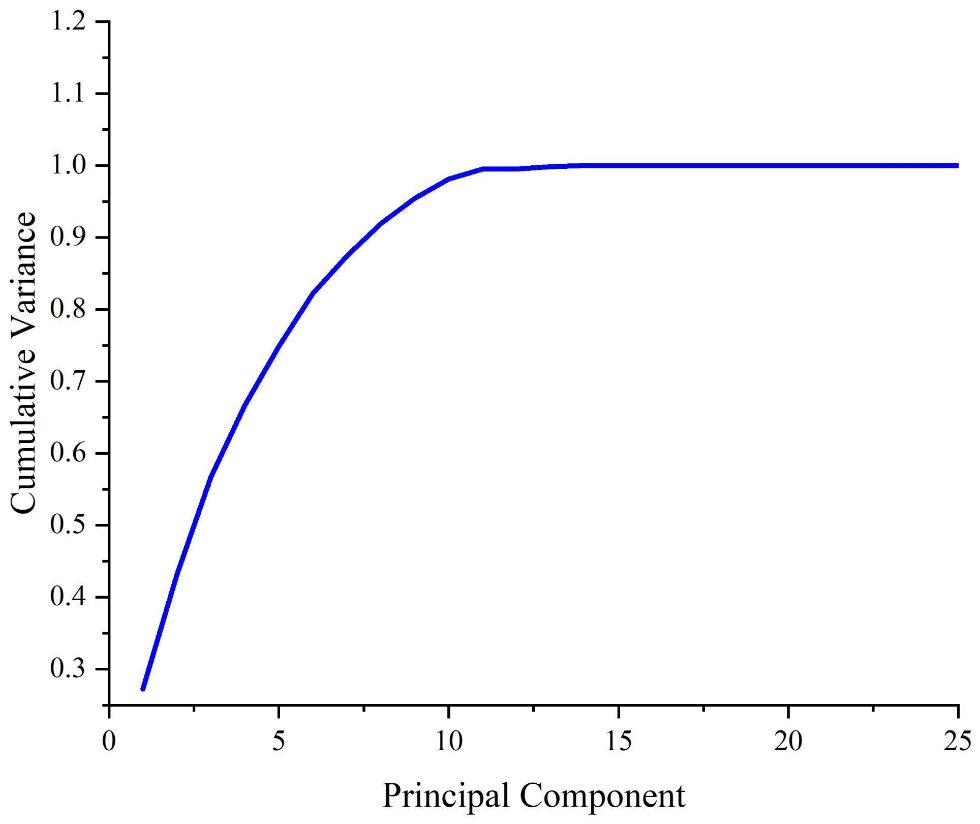
Typically, a subset of principal components is selected so that the cumulative contribution reaches a predefined threshold ${\mathit{\eta }}_{\mathit{PCA}}$, forming the key feature set. The explained variance ratios and cumulative contributions of the retained components are illustrated in Figure 4. It can be noted that electricity market features can be heavy-tailed; therefore, covariance-based PCA may be sensitive to extreme values. To assess robustness, we repeat the PCA under robust preprocessing (e.g., winsorization/robust scaling) and confirm that the leading components and the resulting key feature rankings remain stable.

In addition to conventional system-level parameters such as net load, total generation capacity, ramping limits, and branch flow constraints, the feature space explicitly incorporates indicators related to large-scale renewable integration. These include the renewable penetration ratio at each time interval, forecast errors of wind and photovoltaic units, renewable output ramp rates, and curtailment ratios. By embedding these renewable-related variables into the feature matrix, the PCA-based procedure can capture how symmetry-preserving price patterns are influenced by different renewable operating regimes and how symmetry-breaking anomalies emerge under stressed renewable integration conditions.

Upon establishing compact key feature sets for different types of price anomalies, these sets are used in subsequent structure-consistent driver attribution analysis. PCA is used here for dimensionality reduction and redundancy filtering, and it should not be interpreted as causal variable selection. By matching an anomaly to its corresponding feature set, features with weak correlations can be filtered out, allowing a focus on the most relevant characteristics and avoiding inefficient resource allocation.

4. Causal Attribution of Electricity Price Anomalies

4.1. Influence Functions of Key Features on Electricity Prices

After establishing the key feature sets for different types of price anomalies, further analysis is required to assess the impact of each feature within the set. In this process, the sensitivity of electricity prices to individual feature variables serves as an effective indicator of their influence. However, obtaining accurate sensitivity information requires comprehensive access to market-clearing data, which is not fully disclosed to the public. Nevertheless, as electricity market regulators oversee market operations, they can mandate system operators to provide such information in future market implementations. Once complete market clearing data is available, a multi-parameter optimization approach can be employed to derive the influence functions of key features on electricity prices. Sensitivity analysis based on these influence functions enables the quantification of each feature’s contribution to abnormal price fluctuations.

The process of deriving influence functions using the multi-parameter optimization method is outlined as follows:

First, for ease of formulation, the original optimization problem can be rewritten as:

$$\begin{array}{c}\min \\ \mathrm{w}\in {\mathrm{R}}^{\mathrm{n}}\end{array}{\mathit{A}}^{\mathrm{T}}\mathit{w}$$

(28)

$$s.t. \mathrm{E}\mathrm{w}\le \mathrm{b}:\mathsf{\delta },$$

(29)

where $\mathit{w}$ is the decision variable vector; $\mathit{A}$ is the coefficient matrix in the objective function; $\mathit{E}$ is the coefficient matrix in the constraints; $\mathit{b}$ is the constant vector in the constraints; and $\mathit{\delta }$ is the dual multiplier vector corresponding to the constraints.

Based on Equations (28) and (29), the nodal price expression in Equation (7) can be reformulated as:

$${\lambda }_{k,t}=M_{k,t}\delta ,$$

(30)

where ${\mathit{M}}_{\mathit{k},\mathit{t}}$ represents the coefficient matrix.

The Karush–Kuhn–Tucker (KKT) conditions for the optimization problem [28,29] are given in Equations (31)–(33):

$$A-E^{\top }\delta =0$$

(31)

$$(Ew-b)\odot \delta =0$$

(32)

$$\delta \ge 0$$

(33)

Since the key feature elements exist only in the coefficient matrices $\mathit{A}$ and $\mathit{b}$, the analysis is divided into two cases as follows:

➀

When the feature under investigation is a generator’s bid or a transmission limit penalty factor:

In this case, the constraints can be categorized into active and inactive constraints, as formulated in Equations (34) and (35), based on Equations (29)–(32):

$$E^{\mathit{AC}}w=b^{\mathit{AC}}:{\delta }^{\mathit{AC}}$$

(34)

$$E^{\mathit{DC}}w<b^{\mathit{DC}}:{\delta }^{\mathit{DC}}=0,$$

(35)

where $\left[\right({\mathit{E}}^{\mathit{AC}}{)}^{\top } ({\mathit{E}}^{\mathit{DC}}{)}^{\top }] ={ \mathit{E}}^{\top },$ $\left[\right({\mathit{b}}^{\mathit{AC}}{)}^{\top } ({\mathit{b}}^{\mathit{DC}}{)}^{\top }] ={ \mathit{b}}^{\top },$ and $\left[\right({\mathit{\delta }}^{\mathit{AC}}{)}^{\top } ({\mathit{\delta }}^{\mathit{DC}}{)}^{\top }] ={ \mathit{\delta }}^{\top }$.

Bring ${\mathsf{\delta }}^{\mathrm{DC}} = 0$ into Equation (31), eliminating the dual multipliers corresponding to the non-functioning constraints, and end up with Equation (36):

$$A=(E^{\mathit{AC}}{)}^{\top }{\delta }^{\mathit{AC}}$$

(36)

By the optimality theory [29] where $({\mathit{E}}^{\mathit{AC}}{)}^{\top }$ is a full rank matrix, Equation (36) can be obtained by matrix variation as Equation (37):

$${\delta }^{\mathit{AC}}=\left(\right(E^{\mathit{AC}}{)}^{\top }{)}^{-1}A$$

(37)

The feature under analysis in matrix $\mathit{A}$ is denoted as ${\mathit{A}}^{*}$. From Equation (37), it follows that the dual multipliers associated with active constraints are linear functions of ${\mathit{A}}^{*}$. Since the dual multipliers corresponding to inactive constraints satisfy ${\mathit{\delta }}^{\mathit{DC}} = 0$, they can also be expressed as linear functions of ${\mathit{A}}^{*}$. By combining both cases, the formulation leads to:

$$\delta =k{A}^{*}+g,$$

(38)

where $\mathit{k}$ and $\mathit{g}$ are the vectors derived through transformation and rearrangement.

Substituting Equation (38) into Equation (30) can obtain the nodal price expression as:

$${\lambda }_{k,t}=M_{k,t}(k{A}^{*}+g)$$

(39)

From Equation (39) and the derivation above, it is evident that as long as the set of active constraints in the optimization problem remains unchanged, the nodal price is a linear function of the analyzed feature. Moreover, this linear relationship holds within a specific feasibility region ${\mathit{R}}_{\mathit{j}}$, where the active constraint set remains constant. If the active constraints change, a new linear function is established. Consequently, the final nodal price can be represented as a piecewise linear function of ${\mathit{A}}^{*}$, as formulated in Equation (40):

$$A={\lambda }_{k,t}=\left\{\begin{array}{c}{f}_1\left(A^{*}\right),\forall A^{*}\in {\mathfrak{R}}_1\\ f_2\left(A^{*}\right),\forall A^{*}\in {\mathfrak{R}}_j\\ f_N\left(A^{*}\right),\forall A^{*}\in {\mathfrak{R}}_N\end{array}\right.,$$

(40)

where ${\mathit{f}}_{\mathit{j}}\left({\mathit{A}}^{*}\right)$ represents the functional form of the jth segment of the piecewise linear function.

➁

System constraints as features under analysis

Through applying a similar derivation process, Equation (37) can be obtained. In this scenario, since matrix $\mathit{A}$ remains constant, the dual multipliers associated with the active constraints also remain constant. Given that the dual multipliers for inactive constraints satisfy ${\mathit{\delta }}^{\mathit{DC}} = 0$, it follows that when the set of active constraints remains unchanged, the nodal price is also constant.

Denoting the analyzed feature in vector $\mathit{b}$ as ${\mathit{b}}^{*}$, any variation in ${\mathit{b}}^{*}$ results in a corresponding shift in the set of active constraints in the optimization problem (28) and (29), leading to changes in the nodal price. Ultimately, the nodal price can be expressed as a piecewise constant function in this limiting case, as formulated in Equation (41), which represents a degenerate form of the general piecewise linear price response under fixed active constraints:

$${\mathit{b}}^{*}={\mathit{\lambda }}_{\mathit{k},\mathit{t}}=\left\{\begin{array}{c}{\mathit{q}}_1, \mathit{\forall }{\mathit{b}}^{*}\in {\mathit{R}}_1\\ {\mathit{q}}_{\mathit{j}}, \forall {\mathit{b}}^{*}\in {\mathit{R}}_{\mathit{j}}\\ {\mathit{q}}_{\mathit{N}}, \forall {\mathit{b}}^{*}\in {\mathit{R}}_{\mathit{N}}\end{array}\right.,$$

(41)

where ${\mathit{q}}_{\mathit{j}}$ represents the constant nodal price within the jth feasible region.

Fundamentally, Equation (41) represents a degenerate special case of the piecewise linear price function in Equation (40), arising when marginal price responses vanish under fixed active constraint sets. Both cases are therefore unified within the generalized piecewise linear representation in Equation (42):

$${\lambda }_{k,t}=\left\{\begin{array}{l}{f}_1\left(x_i\right), \forall x_i\in {\mathfrak{R}}_l\\ \dots \\ f_j\left(x_i\right), \forall x_i\in {\mathfrak{R}}_j\\ \dots \\ f_N\left(x_i\right), \forall x_i\in {\mathfrak{R}}_N\end{array}\right.,$$

(42)

where ${\mathit{x}}_{\mathit{i}}$ represents the ith feature in the feature set, and ${\mathit{f}}_{\mathit{j}}\left({\mathit{x}}_{\mathit{i}}\right)$ denotes the functional form of the jth segment of the piecewise linear function.

Based on the above analysis, nodal prices exhibit a piecewise linear relationship with key features, implying that the time-weighted average electricity price follows the same functional form. However, deriving these relationships via multi-parameter optimization is computationally intensive. To mitigate this issue, a sampling-based approach can be employed to approximate the function in Equation (39).

4.2. Causal Analysis Methodology for Abnormal Electricity Prices

Once the key feature sets for different types of abnormal electricity prices have been established, the next step is to match the anomalous price signals, which are subject to causal analysis, with their corresponding key feature sets. The process for calculating the degree of influence and conducting causal analysis is illustrated in Figure 3.

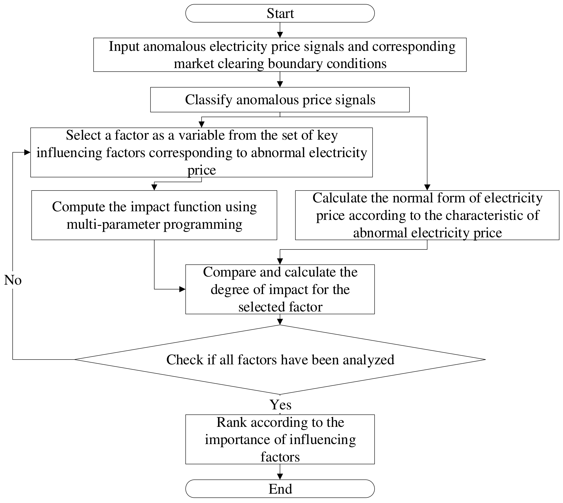
To avoid repetition, the canonical workflow is summarized in Figure 5. In this section, we focus on the implementation details of feature-impact quantification and ranking: (i) deriving reference ranges from normal signals, (ii) matching anomaly-specific key feature sets, and (iii) computing normalized impact coefficients used to produce the final importance ranking for diagnostic attribution.

The resulting ranking of feature importance provides a data-driven basis for designing market and operational interventions that actively support large-scale renewable energy integration (e.g., enhancing flexibility resources, revising congestion management policies, or tuning bidding rules for VRE units).

Section 2, Section 3 and Section 4 describe the general, market-agnostic framework and ranking methodology. Section 5 reports the case study-specific instantiation, including dataset settings, market context, and evaluation protocol.

5. Case Study

This section instantiates the proposed framework on real-world day-ahead market data to demonstrate its diagnostic capability under practical clearing conditions. Detailed data description, variable construction, and preprocessing settings are provided in Section 5.1.

5.1. Data Description and Preprocessing

The empirical analysis is conducted using real-world electricity market data. The dataset spans approximately 1.7 years of continuous operation of the Southern China day-ahead electricity spot market, comprising more than 15,000 hourly market-clearing instances, with nodal electricity prices, load levels, renewable generation outputs, and network-related indicators collected at an hourly resolution. The selected market operates under a centralized market-clearing mechanism with locational marginal pricing, making it suitable for KKT-based price interpretation.

Key explanatory variables are constructed to capture demand conditions, renewable penetration, and network stress. Specifically, load-related features are derived from nodal demand levels and their temporal variations; renewable-related indicators include wind and photovoltaic output ratios and ramping magnitudes; and network-related features are represented by congestion indicators and binding constraint proxies extracted from market-clearing results.

Prior to analysis, data preprocessing is performed to ensure numerical stability and comparability. Missing values, which account for less than 1% of the observations, are handled using median imputation. All continuous variables are standardized using z-score normalization. Extreme outliers beyond the 99.5th percentile are retained for anomaly analysis but excluded from normalization parameter estimation to avoid distortion.

Based on the classification criteria described in Section 3, the dataset yields N₁ price spike anomaly cases, N₂ mean-shift anomaly cases, and N₃ normal operation cases, which are used for subsequent attribution analysis.

5.2. Construction of Key Characteristic Sets for Electricity Price Anomalies

The anomaly classification method described in Section 3.1 was applied to approximately 15,000 sets of electricity price clearing data. Since different manifestations of the same anomaly category may result from distinct influencing factors, a further refinement of the anomaly classification was conducted. Specifically, price spike anomalies were divided into upward price spikes and downward price spikes. This classification resulted in two datasets: approximately 12,000 instances of upward price spikes and 18,000 instances of downward price spikes. Principal component analysis (PCA) was performed to identify the key influencing factors for these two types of anomalies, as summarized in

Table 2. Key features of the electricity price spike anomaly scenarios.

Order	Electricity Prices Up and Under the Spike
1	Branch power flow limit ratio
2	Net load
3	Total generation capacity
4	Load variation compared to the previous time period
5	Load variation compared to the subsequent time period
6	Maximum bid price
7	Minimum bid price

.

A similar approach was applied to mean price anomalies, which were further classified into excessively high and excessively low mean prices. This refinement yielded approximately 2400 instances of high mean price anomalies and 2700 instances of low mean price anomalies. The application of PCA extracted the key influencing factors for these two subcategories, as presented in

Table 3. A collection of key features of mean price anomalies.

Order	Excessively High Mean Value	Excessively Low Mean Value
1	Average net load	Average net load
2	Load peak-to-valley difference	Load peak-to-valley difference
3	Total generation capacity	Total generation capacity
4	Total minimum generation output	Maximum load ramp-up
5	Violation count of branch power flow constraints	Maximum load ramp-down
6	Unit ramp capability	Maximum unit bid price
7	Penalty factor for power flow constraint violations	Average unit bid price

. Notably, for mean price anomalies, the distinction between key influencing factors across different manifestations of the anomaly is even more pronounced.

The key features extracted through PCA include system-wide parameters from both market and non-market units. While non-market units are not economically dispatched, their generation limits, ramping capabilities, and minimum output values influence system dynamics and thus play a critical role in shaping abnormal price behaviors.

5.3. Validation of the Causal Tracing Process for Electricity Price Anomalies

To illustrate the proposed causality tracing method, a specific case of excessively high mean price anomalies is analyzed. In this case, the average electricity price reaches 856.52 CNY/MWh. However, statistical analysis of the generated data reveals that in over 5% of cases, the mean electricity price exceeds 300 CNY/MWh, which is considered the upper threshold for the normal range of mean prices.

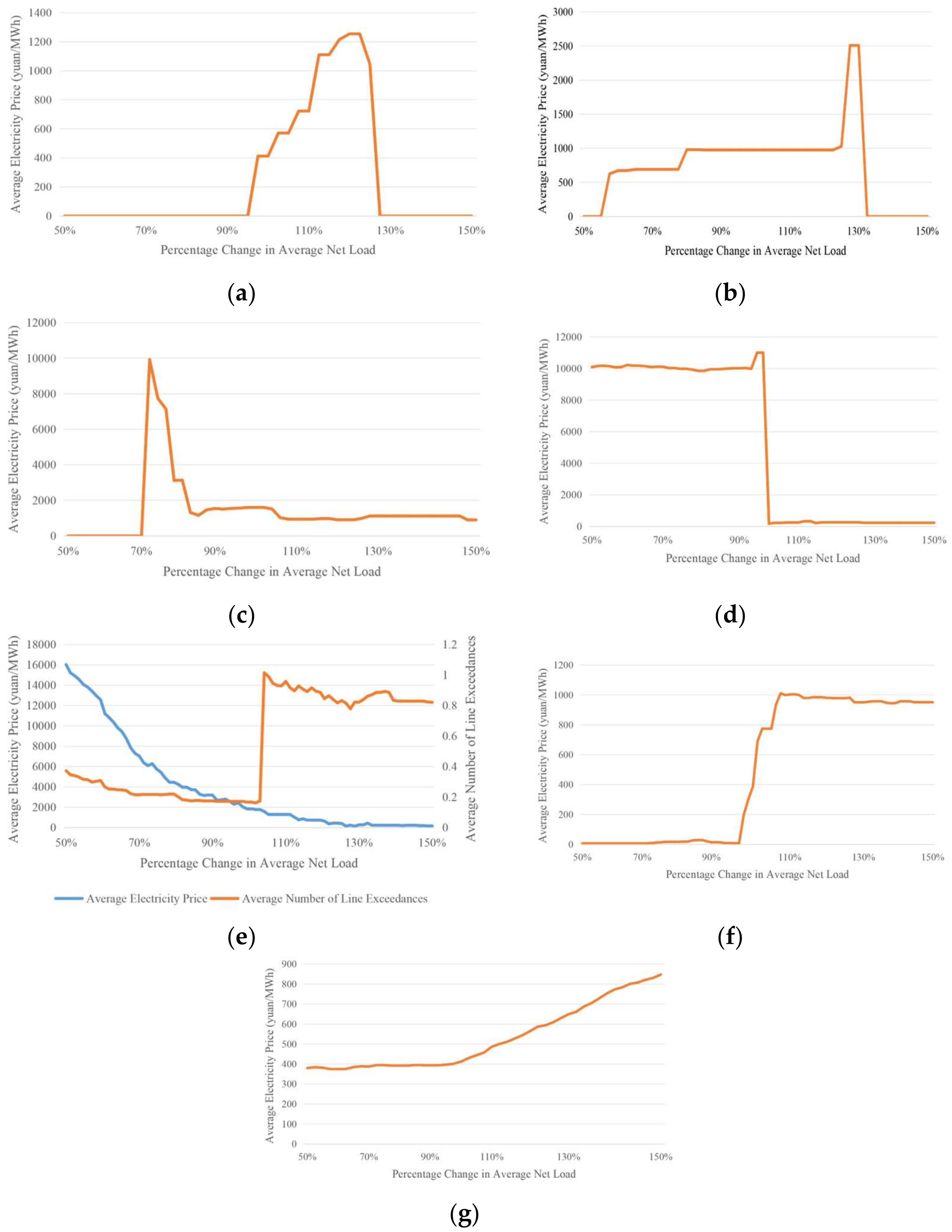
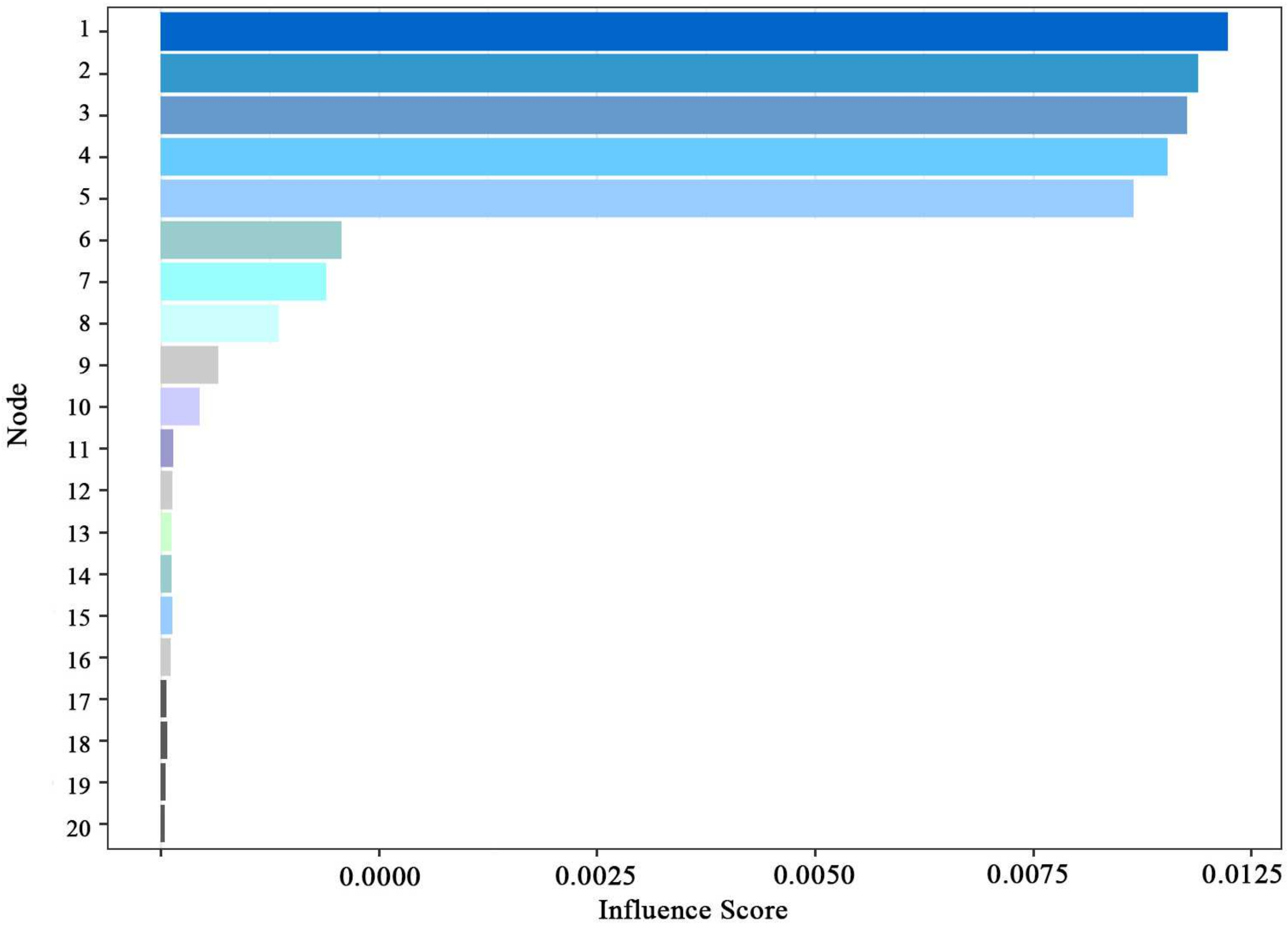
Following the key features identified for the “excessively high mean” anomaly type, as listed in

Table 4. The degree to which each feature influences the average electricity price.

Order	Key Features	Absolute Value of the Percent Change in Feature	Contribution Arranged in Order
1	Average net load	Approximately equal to 10%	1
2	Peak-to-valley variation in load	Greater than 44%	3
3	Total unit capacity	Greater than 50%	4
4	Total minimum output of the unit	Not very relevant	7
5	Upper and lower limits of branch power flow	Approximately equal to 14%	2
6	Ramping capability of the unit	Much greater than 50%	6
7	Power flow constraint violation penalty factor	Much greater than 50%	5

, the functional representations of electricity price averages concerning each key feature are obtained sequentially, as depicted in Figure 6. Figure 7 visualizes the influence-ranking results, highlighting the dominant drivers associated with each anomaly type.

Figure 6 presents the functional relationships between the mean electricity price in this anomaly case and various influencing factors, including average net load variation, load peak-to-valley difference, generation capacity variation, lower generation output limits, branch capacity constraints, ramping coefficients, and penalty factors for power flow constraint violations. Instances where the electricity price is zero indicate infeasibility in the clearing process. Sensitivity analysis is then conducted to quantify the impact of each feature on the mean electricity price, with the results summarized in Table 3.

The contribution analysis highlights that, in this particular anomaly case, the mean electricity price is most sensitive to variations in average net load, followed by branch power flow constraints. As shown in Figure 6e, changes in the number of power flow constraint violations are neither sufficiently pronounced nor easily quantifiable. Therefore, an alternative analysis is performed using the upper and lower limits of branch power flow constraints. Beyond these two dominant factors, the influence of other features on the mean electricity price is relatively minor, aligning well with insights derived from manual judgment. The selected case with excessively high mean prices corresponds to a period with an hourly renewable penetration level exceeding 50% of total generation during peak wind and photovoltaic output periods, accompanied by significant wind power ramps and repeated congestion on major export corridors. Under such conditions, the proposed symmetry-guided causal tracing framework indicates that the dominant drivers of the anomaly are the combination of elevated net load after accounting for renewable variability and binding transmission constraints in renewable-rich areas. This finding suggests that targeted investments in grid reinforcement and flexible resources (such as storage or demand response) would be more effective for supporting renewable integration than simply tightening bidding caps.

5.4. Accuracy Verification of Causal Tracing for Abnormal Electricity Prices

To improve transparency and verifiability, an expert-based benchmark is used to evaluate the diagnostic performance of the proposed framework. The benchmark consists of three independent experts with over 5 years of experience in electricity spot market operation and price anomaly analysis. For each selected anomaly case, experts were provided with the corresponding nodal price trajectories and market-clearing summaries, including relevant load, renewable output, and network constraint information. Without access to model results, each expert independently identified the dominant drivers of the observed price anomaly based on professional judgment.

The framework’s performance is evaluated using an agreement rate with expert assessments rather than statistical predictive accuracy. An attribution result is considered consistent if the top-ranked dominant factor identified by the framework matches the primary factor agreed upon by the experts. Under this definition, the reported 90% and 85% values represent diagnostic consistency for price spikes and mean price anomalies, respectively.

To validate the effectiveness of the proposed method, 40 representative cases (including 20 price spike anomalies and 20 mean price anomalies) were selected from the electricity spot market dataset. These cases were identified from multi-day actual nodal price trajectories. Specifically, the expert benchmark was formed by a panel of three senior market analysts from the regional system operator and market supervision departments, each with more than 5 years of experience in spot market operation and price anomaly assessment. For each selected anomaly case, experts independently identified the primary influencing factors based on full access to market operation reports and clearing summaries, without referring to the model outputs. Additionally, 10 cases of price spike anomalies and 10 cases of mean price anomalies were chosen from the data. The results were compared against those obtained through expert judgment to assess the accuracy of the causal tracing process.

The causal tracing results for abnormal electricity prices are presented in

Table 5. Causal tracing results for price spike anomalies.

Order	Tracing Results of the Proposed Method	Manual Judgment Tracing Results	Order	Traceability Results of the Proposed Method	Artificial Empirical Traceability Results
1	Load level	Load level	11	Load variation relative to the next time period	Load variation relative to the next time period
2	Load variation between consecutive time periods	Load variation between consecutive time periods	12	Change in load from previous time period	Load level, change in load between pre and post time periods
3	Branch power flow limit ratio	Branch power flow upper and lower limits	13	Load variation relative to the previous time period	Load variation relative to the previous time period
4	Load variation between consecutive time periods	Load variation between consecutive time periods	14	Load variation between consecutive time periods, branch power flow limit ratio	Load level, load variation between consecutive time periods
5	Branch power flow limit ratio, load variation between consecutive time periods	Load variation between consecutive time periods	15	Load variation between consecutive time periods	Load level, load variation between consecutive time periods
6	Load variation between consecutive time periods	Load level, load variation between consecutive time periods, branch power flow upper and lower limits	16	Load variation relative to the previous time period	Load variation relative to the previous time period
7	Load variation relative to the previous time period	Load variation between consecutive time periods	17	Load level	Upper and lower limits of branch flow, load variation relative to the previous time period
8	Load level	Load variation relative to the previous time period	18	Load level	Upper and lower limits of branch flow, load levels, load variation relative to the next time period
9	Load variation relative to the previous time period	Load level, load variation between consecutive time periods, Branch power flow upper and lower limits	19	Load variation relative to the previous time period	Upper and lower limits of branch flow, load levels
10	Load variation between consecutive time periods	Load variation between consecutive time periods	20	Load variation relative to the next time period	Load variation relative to the next time period

and

Table 6. Cause analysis results for price mean anomalies.

Order	Traceability Results of the Proposed Method	Artificial Empirical Traceability Results	Order	Traceability Results of the Proposed Method	Artificial Empirical Traceability Results
1	Branch power flow upper and lower limits, average net load, load peak-to-valley difference, penalty factor for power flow constraint violations	Branch power flow upper and lower limits, low supply–demand balance, load peak-to-valley difference, penalty factor for power flow constraint violations	11	Average net load, total unit capacity	High supply–demand ratio
2	Average net load, branch power flow upper and lower limits	Branch power flow upper and lower limits, low supply–demand balance	12	Average net load, total unit capacity	High supply–demand ratio
3	Average net load, load peak-to-valley differential, ramp capability of generating units, penalty factor for power flow constraint violations	Branch power flow upper and lower limits, low supply–demand balance, and penalty factor for power flow constraint violations	13	Average net load, quoted average	High supply–demand ratio, average value of offers
4	Average net load, upper and lower branch current limits	Average net load, load peak-to-valley difference, upper and lower limits of branch power flows	14	Average net load, quoted average	High supply–demand ratio, average value of offers
5	Average net load, upper and lower branch circuit power flow limits, unit ramping capability	Average net load, upper and lower branch power flow limits, power constraint overrun penalty factor	15	Average net load, unit total capacity, quoted average value	High supply–demand ratio, average value of offers
6	Upper and lower limits of branch power flows	Low supply–demand ratio	16	Average net load, unit total capacity quoted average value	High supply–demand ratio, average value of offers
7	Average net load, upper and lower branch current limits, total unit capacity	Lower supply–demand ratio, upper and lower branch power flow limits	17	Average net load	High supply–demand ratio
8	Upper and lower limits of branch power flows	Upper and lower limits of branch power flows	18	Average net load, total unit capacity	High supply–demand ratio
9	Upper and lower limits of branch power flows	Upper and lower limits of branch power flows	19	Average net load, total unit capacity	High supply–demand ratio
10	Average net load	Upper and lower limits of branch power flows	20	Total unit capacity, average net load	High supply–demand ratio, average value of offers

. For price spike anomalies, the proposed framework produced the same primary influencing factor as the expert consensus in approximately 90% of the cases. For mean price anomalies, the consistency rate with expert-identified dominant drivers was approximately 85%. Here, consistency is defined as the agreement on the top-ranked influencing factor rather than exact matching of full factor rankings.

From Table 5, it can be found that for electricity price spike anomalies, the formation causes are more concentrated, the electricity price signal is more sensitive to the elements in the key influence set, and the proposed method can identify the main influencing factors more sensitively, while the manual empirical method cannot do a precise analysis of the data, and therefore the traceability results usually have a wider range. Overall, for electricity price spike anomalies, the traceability results of the proposed method in this paper are consistent with the manual method in about 90% of the cases.

From Table 6, it can be found that for the mean anomaly, the formation causes will be more complicated, and when the mean price anomaly is traced through the method proposed in this paper, about 85% of the cases get the same traceability results as the manual empirical method.

In summary, the comprehensive traceability accuracy of the method proposed in this paper reaches more than 85%, and, at the same time, relative to the manual empirical method, it can give a scientific and objective ordering of the contribution of the influencing factors, so that the traceability results of the causes of electricity price anomalies can be based on the evidence and traces. These results demonstrate the effectiveness of the proposed framework in diagnosing and attributing dominant structural drivers associated with electricity price anomalies under observed market-clearing conditions.

6. Conclusions

A symmetry-guided analytical framework is proposed to diagnose and trace electricity price anomalies by distinguishing symmetry-preserving normal states from symmetry-breaking abnormal states. By combining PCA—based feature compaction with a structure-consistent influence ranking method, the framework identifies the dominant factors underlying different anomaly types in a transparent manner without relying on black-box models or extensive historical data. Case studies on real market data show that the resulting attributions are broadly consistent with expert assessments. Overall, the analysis suggests that most price anomalies can be explained by a small set of structurally interpretable drivers—primarily congestion, scarcity, and renewable-related stress conditions—providing practical insights for market monitoring and regulatory assessment. The results should be interpreted as mechanism-based diagnostic evidence rather than interventional causal claims, and applications to other markets require adaptation to local rules and network structures.

References

1. Deng, W.; Xiao, D.; Chen, M.; Tahir, M.F.; Zhu, D. Multi-Regional Energy Sharing Approach for Shared Energy Storage and Local Renewable Energy Resources Considering Efficiency Optimization. Int. J. Electr. Power Energy Syst. 2025, 167, 110592. [Google Scholar] [CrossRef]
2. Ahsan, F.; Dana, N.H.; Sarker, S.K. Data-Driven Next-Generation Smart Grid Towards Sustainable Energy Evolution: Techniques and Technology Review. Prot. Control Mod. Power Syst. 2023, 8, 43. [Google Scholar] [CrossRef]
3. Li, J.; Mu, G.; Zhang, J. Dynamic Economic Evaluation of Hundred Megawatt-Scale Electrochemical Energy Storage for Auxiliary Peak Shaving. Prot. Control Mod. Power Syst. 2023, 8, 50. [Google Scholar] [CrossRef]
4. Chen, Y.; Zhang, L.; Xu, P.; Di Gangi, A. Electricity Demand Response Schemes in China: Pilot Study and Future Outlook. Energy 2021, 224, 120042. [Google Scholar] [CrossRef]
5. Li, G.; Gao, D.; Li, Y. Impacts of Market-Based Environmental Regulation on Green Total Factor Energy Efficiency in China. China World Econ. 2023, 31, 92–114. [Google Scholar] [CrossRef]
6. Laitsos, V.; Vontzos, G.; Paraschoudis, P.; Tsampasis, E.; Bargiotas, D.; Tsoukalas, L.H. The State of the Art Electricity Load and Price Forecasting for the Modern Wholesale Electricity Market. Energies 2024, 17, 5797. [Google Scholar] [CrossRef]
7. Pinhão, M.; Fonseca, M.; Covas, R. Electricity Spot Price Forecast by Modelling Supply and Demand Curve. Mathematics 2022, 10, 2012. [Google Scholar] [CrossRef]
8. Habib, M.A. Game Theory, Electrical Power Market and Dilemmas. J. Electr. Eng. Electron. Control Comput. Sci. 2022, 8, 33–42. [Google Scholar]
9. Zhuo, Z.; Du, E.; Zhang, N.; Nielsen, C.P.; Lu, X.; Xiao, J.; Kang, C. Cost Increase in the Electricity Supply to Achieve Carbon Neutrality in China. Nat. Commun. 2022, 13, 3172. [Google Scholar] [CrossRef]
10. Peura, H.; Bunn, D.W. Renewable Power and Electricity Prices: The Impact of Forward Markets. Manag. Sci. 2021, 67, 4772–4788. [Google Scholar] [CrossRef]
11. Gabrielli, P.; Wüthrich, M.; Blume, S.; Sansavini, G. Data-Driven Modeling for Long-Term Electricity Price Forecasting. Energy 2022, 244, 123107. [Google Scholar] [CrossRef]
12. Bao, M.; Ding, Y.; Zhou, X.; Guo, C.; Shao, C. Risk Assessment and Management of Electricity Markets: A Review with Suggestions. CSEE J. Power Energy Syst. 2021, 7, 1322–1333. [Google Scholar] [CrossRef]
13. Cicala, S. Imperfect Markets versus Imperfect Regulation in US Electricity Generation. Am. Econ. Rev. 2022, 112, 409–441. [Google Scholar] [CrossRef]
14. Chen, H.; Cui, J.; Song, F.; Jiang, Z. Evaluating the Impacts of Reforming and Integrating China’s Electricity Sector. Energy Econ. 2022, 108, 105912. [Google Scholar] [CrossRef]
15. Bjarghov, S.; Löschenbrand, M.; Saif, A.I.; Pedrero, R.A.; Pfeiffer, C.; Khadem, S.K.; Farahmand, H. Developments and Challenges in Local Electricity Markets: A Comprehensive Review. IEEE Access 2021, 9, 58910–58943. [Google Scholar] [CrossRef]
16. Ejuh Che, E.; Roland Abeng, K.; Iweh, C.D.; Tsekouras, G.J.; Fopah-Lele, A. The impact of integrating variable renewable energy sources into grid-connected power systems: Challenges, mitigation strategies, and prospects. Energies 2025, 18, 689. [Google Scholar] [CrossRef]
17. Cao, Y.; Xu, B.; Zhang, C.; Li, F.F.; Liu, Z. Strategic site-level planning of VRE integration in hydro-wind-solar systems under uncertainty. Energy 2025, 328, 136523. [Google Scholar] [CrossRef]
18. Doering, K.; Sendelbach, L.; Steinschneider, S.; Anderson, C.L. The effects of wind generation and other market determinants on price spikes. Appl. Energy 2021, 300, 117316. [Google Scholar] [CrossRef]
19. Dai, S.; Wang, J.; Ji, T. Symmetry-Guided Identification of Spatial Electricity Price Anomalies via Data Partitioning and Density Analysis. Symmetry 2025, 17, 1032. [Google Scholar] [CrossRef]
20. Ramos, S.; Soares, J.; Cembranel, S.S.; Tavares, I.; Foroozandeh, Z.; Vale, Z.; Fernandes, R. Data mining techniques for electricity customer characterization. Procedia Comput. Sci. 2021, 186, 475–488. [Google Scholar] [CrossRef]
21. Si, C.; Xu, S.; Wan, C.; Chen, D.; Cui, W.; Zhao, J. Electric Load Clustering in Smart Grid: Methodologies, Applications, and Future Trends. J. Mod. Power Syst. Clean Energy 2021, 9, 237–252. [Google Scholar] [CrossRef]
22. Durante, F.; Gianfreda, A.; Ravazzolo, F.; Rossini, L. A Multivariate Dependence Analysis for Electricity Prices, Demand and Renewable Energy Sources. Inf. Sci. 2022, 590, 74–89. [Google Scholar] [CrossRef]
23. Tehrani, S.; Juan, J.; Caro, E. Electricity Spot Price Modeling and Forecasting in European Markets. Energies 2022, 15, 5980. [Google Scholar] [CrossRef]
24. Jain, M.; Sun, X.; Datta, S.; Somani, A. A Machine Learning Framework to Deconstruct the Primary Drivers for Electricity Market Price Events. In Proceedings of the 2023 IEEE Power & Energy Society General Meeting (PESGM), Orlando, FL, USA, 16–20 July 2023; IEEE: New York, NY, USA, 2023; pp. 1–5. [Google Scholar]
25. Bâra, A.; Oprea, S.V. Predicting Day-Ahead Electricity Market Prices through the Integration of Macroeconomic Factors and Machine Learning Techniques. Int. J. Comput. Intell. Syst. 2024, 17, 10. [Google Scholar] [CrossRef]
26. Mahler, V.; Girard, R.; Kariniotakis, G. Data-Driven Structural Modeling of Electricity Price Dynamics. Energy Econ. 2022, 107, 105811. [Google Scholar] [CrossRef]
27. Yang, W.; Sun, S.; Hao, Y.; Wang, S. A Novel Machine Learning-Based Electricity Price Forecasting Model Based on Optimal Model Selection Strategy. Energy 2022, 238, 121989. [Google Scholar] [CrossRef]
28. Yang, Y.S.; Xie, B.C.; Tan, X. Impact of Green Power Trading Mechanism on Power Generation and Interregional Transmission in China. Energy Policy 2024, 189, 114088. [Google Scholar] [CrossRef]
29. Li, G.; Du, G.; Liu, G.; Yan, J. Study on the Dynamic Characteristics, Control Strategies and Load Variation Rates of the Concentrated Solar Power Plant. Appl. Energy 2024, 357, 122538. [Google Scholar] [CrossRef]
Figure 1. Schematic diagram of existing price assessment framework.
Symmetry 18 00390 g001
Figure 2. Illustrative methodology for causal attribution of price anomalies based on key feature comparison.
Symmetry 18 00390 g002
Figure 3. Histogram of electricity spot price.
Symmetry 18 00390 g003
Figure 4. Explained variance ratios and cumulative contributions of principal components.
Symmetry 18 00390 g004
Figure 5. Flowchart for feature importance ranking using an alternative algorithm.
Symmetry 18 00390 g005
Figure 6. Functional relationships between mean electricity price and key features over the scheduling period. (a) Functional relationship between mean electricity price and average load variation. (b) Functional relationship between mean electricity price and load peak-to-valley difference. (c) Functional relationship between mean electricity price and generation capacity variation. (d) Functional relationship between mean electricity price and upper and lower generation output limits. (e) Functional relationship between mean electricity price and upper and lower branch capacity limits. (f) Functional relationship between mean electricity price and unit ramping coefficient variation. (g) Functional relationship between mean electricity price and penalty factor for power flow constraint violations.
Symmetry 18 00390 g006
Figure 7. Functional relationships between mean electricity price and key features over the scheduling period.
Symmetry 18 00390 g007