Safe Trajectory Tracking for Robotic Manipulator with Prescribed Performance in Confined Spaces

Abstract

This paper addresses the issue of safe trajectory tracking for robotic manipulators operating in confined spaces that often exhibit asymmetric geometric structures, such as narrow passages or cluttered obstacle fields. We introduce an innovative model-free control strategy aimed at guaranteeing safe trajectory tracking by constraining joint trajectory tracking errors within prescribed safe bounds. To achieve the desired tracking objective, an error transformation mechanism is developed. Notably, the robustness of this mechanism against model uncertainties eliminates the necessity for knowledge of the system model, enabling model-free control. Additionally, we introduce a Monte Carlo-based search strategy that integrates motion planning, which provides a collision-free feasible reference trajectory, with control, which ensures runtime safety. This framework operates autonomously and guarantees safety at both the planning and control layers. The controller’s robustness, along with its autonomous implementation from planning to control, facilitates practical deployment in complex real-world environments and is effectively validated on a Baxter robotic platform.

1. Introduction

Safety is important for robotic manipulators performing tasks in the environment with obstacles, such as the requirement to navigate through confined and narrow spaces or dense obstacles. In these scenarios, the planned trajectory often brings the manipulator into close proximity to nearby obstacles [1,2], thereby increasing the risk of collisions during execution. Hence, it is essential to consider safe trajectory tracking to mitigate potential risks and hazards.

Before performing safe trajectory tracking, it is essential to first generate a collision-free reference trajectory. In previous studies on safe trajectory tracking of robotic manipulator, the generation of reference trajectories has often been considered only at the control level, with methods either unspecified [3,4] or entirely manually defined [5,6]. Such approaches are limited, as the reference trajectories themselves may contain potential collision risks or workspace constraints, which cannot fully ensure the safety of the manipulator in complex environments. To address this issue, the present study introduces motion planning methods, such as sampling-based algorithms [7] or the A* algorithm [8], at the planning level to autonomously generate collision-free reference trajectories based on the actual environment and obstacle distribution. These trajectories then provide a safe and feasible foundation for subsequent control-level trajectory tracking. This top-down integration of planning and control not only ensures motion safety but also enhances the manipulator’s autonomy in navigating complex workspaces.

Some control strategies ensure the safety of the robot or the environment from the perspective of reducing the contact force between the robot and the environment, such as the use of passive torque limiters [5] and trajectory scaling to adjust the time stamp [9]. However, the robotic manipulator is forced to halt its motion until the surrounding obstacles are removed, potentially hindering the efficient completion of planned tasks. Additionally, the aforementioned methods require costly force sensors either in the end-effector or the joints. To ensure the robotic manipulator can safely and reliably follow the planned trajectory, constraints need to be imposed on the trajectory tracking performance. Fixed-Time Control (FTC) [10,11,12] enables tracking errors convergence to near zero within a predetermined fixed time, thereby providing faster convergence capability and better transient performance. However, such control strategies are unable to directly specify the tracking error of the trajectory. Currently, typical control methods for specifying tracking error include Barrier Lyapunov Function (BLF)-based control and Prescribed Performance Control (PPC) [13,14].

The control design methods based on the Barrier Lyapunov Function (BLF) effectively handle constrained tracking errors. The core idea is that as the tracking error nears specific boundary regions, the BLF value approaches infinity. By ensuring the boundedness of BLF, the goal of limiting tracking errors can be attained [15]. However, the performance of BLF-based methods inherently relies on explicit system models, which are often difficult to obtain in practical scenarios. Even for well-structured rigid robotic manipulators, considerable parametric uncertainties may still arise [16]. To address these uncertainties, additional function approximation mechanisms such as neural networks are typically incorporated [17]. In such approaches, a neural network is first used to approximate the unknown system dynamics, and a BLF-based controller is subsequently designed on the basis of the approximated model to enforce the required constraints [17,18,19,20]. Furthermore, any modification to the BLF formulation within the Lyapunov function requires a complete redesign of the controller together with the reestablishment of the closed-loop stability conditions, which significantly limits the flexibility of BLF-based schemes.

In contrast to BLF-based control, the PPC-based control prescribe performance boundary functions to ensure steady-state performance [14]. Therefore, the control problem of constrained systems is transformed into the state-bounded stabilization control problem of the unconstrained system after mapping. This method recently introduced by Greek scholars Bechlioulis and Rovithakis [21]. Furthermore, by incorporating adaptive mechanisms [22] or approximation frameworks [23,24], many enhanced variants of PPC have been developed for a broad class of nonlinear systems, including robotic manipulators [24,25] and aircraft systems [26,27]. These approaches, however, introduce additional structural complexity due to the parameter learning and tuning procedures required by intelligent control components, which significantly increases computational burden. To alleviate these difficulties, several approximation-free and model-free PPC methods have been proposed based on error transformation techniques [25,28]. Although these methods simplify the controller design and reduce computational demand, they still require the redesign or reselection of certain control parameters whenever a new task is assigned. This lack of task-level adaptability limits their convenience and practicality in real robotic applications. Therefore, it is essential to design a model-free PPC controller that is both structurally simple and robust.

The PPC control method imposes boundary functions on tracking errors, ensuring that the controlled system’s tracking errors always remain within specified bounds [21]. In this study, manipulators executing geometric trajectories in spatially constrained environments with obstacles face restricted motion ranges. Fortunately, predefined performance boundaries guarantee the manipulators operate safely within these constraints. Specifically, by setting performance boundaries for trajectory tracking errors, the method prevents the manipulators from exceeding the allowed spatial boundaries, thus mitigating collision risks and ensuring the safety of both the manipulators and their surrounding environment. However, the principle for autonomously determining safe error boundaries within PPC-based controllers to guarantee safe trajectory tracking is still lacking.

Based on the discussions above, this paper focuses on the issue of safe trajectory tracking for robotic manipulators operating in confined and narrow spaces. By specifying predefined safety boundaries for trajectory tracking errors, it guarantees the safety of trajectory execution. The main contributions are as follows.

(i)

This paper presents novel and robust model-free control method for robotic manipulators to tackle the aforementioned challenge. By leveraging the potential robustness of error transformation techniques, it eliminates the necessity for the robotic manipulators’ model knowledge [29], thereby achieving model-free tracking control;

(ii)

The proposed controller features a simple and implementation-friendly structure, requiring neither adaptive techniques [30,31,32,33,34] nor approximation-based components such as neural networks [35,36] or fuzzy logic systems [37,38]. This structural simplicity makes the controller easier to tune, and highly suitable for practical deployment on real robotic platforms.

(iii)

This work introduces a unified safe trajectory tracking framework that couples motion planning with control through a Monte Carlo–based search of configuration-dependent error bounds. This integration ensures safety at both the planning and control layers, allowing the reference trajectory and its admissible error bounds to be autonomously determined based on the geometric structure of the surrounding environment.

The subsequent organization of the paper is as follows. Section 2 presents a common system description for robotic manipulators and provides the problem to be addressed. In Section 3, the method of solving the above problem is firstly introduced. Based on this, Section 4 designs a controller. Then, in Section 5, the stability of the controller is proven. Subsequently, in Section 6, the effectiveness of the designed control is validated through trajectory tracking experiments with real robotic manipulators. Finally, Section 7 provides conclusions and suggestions for future work.

2. System Description and Problem Formulation

2.1. System Description

Before proceeding with the problem formulation, it is essential to first describe the system model of the research object. As in Ref. [39], the widely adopted dynamic model for robotic manipulators can be expressed as follows:

$$\mathit{M}\left(\mathit{q}\right)\ddot{\mathit{q}}\left(t\right)+\mathit{C}(\mathit{q},\dot{\mathit{q}})\dot{\mathit{q}}\left(t\right)+\mathit{N}(\mathit{q},\dot{\mathit{q}})+\mathit{D}\left(t\right)=\mathit{\tau }\left(t\right)$$

(1)

where $\mathit{q}\left(t\right),\dot{\mathit{q}}\left(t\right),\ddot{\mathit{q}}\left(t\right)\in {\mathbb{R}}^n$ represent the vectors for joint angle, joint velocity, and joint acceleration, respectively; $\mathit{M}\left(\mathit{q}\right)\in {\mathbb{R}}^{n\times n}$ is the inertia matrix of robot; $\mathit{C}(\mathit{q},\dot{\mathit{q}})\in {\mathbb{R}}^{n\times n}$ is the Coriolis and centripetal matrix; $\mathit{N}(\mathit{q},\dot{\mathit{q}})\in {\mathbb{R}}^n$ includes gravity and other forces acting on the robot’s joints; $\mathit{D}\left(t\right)\in {\mathbb{R}}^n$ is the joint disturbance vector; $\mathit{\tau }\left(t\right)\in {\mathbb{R}}^n$ is the joint torque vector; and n is the number of joints in the robot. Considering the inherent characteristics of the system and aiming to streamline subsequent stability analyses, we introduce the following lemmas and assumptions.

Lemma 1 

([39]). The inertia matrix $\mathit{M}\left(\mathit{q}\right)$ in the dynamics equation of system (1) is symmetric and positive definite. Consequently, $\mathit{M}{\left(\mathit{q}\right)}^{-1}$ is bounded.

Assumption 1 

([25,40]). The joint angles $\mathit{q}\left(t\right)$ and joint angular velocities $\dot{\mathit{q}}\left(t\right)$ in system (1) are bounded and measurable.

Assumption 2 

([23,25]). The disturbance $\mathit{D}\left(t\right)$ in system (1) is bounded.

Assumption 3 

([41,42]). If $\mathit{q}\left(t\right)$ and $\dot{\mathit{q}}\left(t\right)$ are bounded, then $\mathit{C}(\mathit{q},\dot{\mathit{q}})$ and $\mathit{N}(\mathit{q},\dot{\mathit{q}})$ are also bounded.

Assumption 4 

([17,18,25]). The reference trajectories $q_{dj}$ and their derivatives ${\dot{q}}_{dj},j=1,\dots ,n$, are bounded.

2.2. Problem Formulation

For the system described in Equation (1), the control objective is to ensure the system’s output joint trajectory $q_j$ closely follow the planned reference joint trajectory $q_{dj}$. The tracking error is defined as

$$e_j\left(t\right)=q_j\left(t\right)-q_{dj}\left(t\right),j=1,\cdots ,n.$$

(2)

To avoid collisions between the robot and surrounding obstacles during the execution of planned trajectory in confined spaces, constraints required to be imposed on the trajectory tracking error.

Based on the given system and assumptions, the specific problem to be investigated can be summarized as follows.

Problem 1.

Consider a robotic manipulator with unknown nonlinear dynamics operating in confined spaces as described in Equation (1), the objective is to design a simple state feedback controller that enables the system to track the reference trajectory with the specified error bounds $w_{1j}$

$$\left|e_j\left(t\right)\right|\le w_{1j},t>0,j=1,\cdots ,n,$$

(3)

where $w_{1j}$ are positive constants.

To address the above problem, our method integrates motion planning with control design in a unified manner. The planning module generates a collision-free reference trajectory together with admissible error bounds $e_j$, while the control strategy ensures that the tracking process strictly satisfies the constraint given in Equation (3) of Problem 1. In the subsequent section, we provide a detailed description of the implementation of this integrated methodology.

3. Method

3.1. Overview of Algorithm

The proposed safe trajectory tracking framework integrates motion planning and control, where the tracking controller relies on the collision-free reference trajectory and corresponding safety bounds obtained from the planning stage. Therefore, before detailing the controller design, we provide an overview of the entire workflow, as shown in Figure 1.

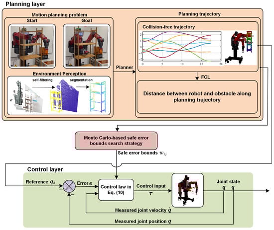
Figure 1. The workflow of the safe trajectory tracking in the confined space.

To begin with, the reference trajectory is generated by a motion planning algorithm tailored to the task at hand. This requires specifying the start and goal configurations, together with a geometric description of all obstacles in the environment. The planner then computes a feasible, collision-free path in the configuration space (C-space), which is subsequently parameterized into a joint-space trajectory.

For each waypoint along this trajectory, the Fast Collision Library (FCL) [43] is employed to evaluate the minimum distances between the manipulator and all surrounding obstacles. Using these distance evaluations, a Monte Carlo–based search procedure is executed along the planned trajectory to determine a set of safe error bounds, denoted as $w_{1j},j=1,\dots ,n$. These bounds encode the allowable deviation of each joint from its reference path and serve as a key input to the controller.

By enforcing these bounds during execution, the designed new controller ensures that the manipulator remains within a provably safe tube around the reference trajectory, thereby preventing potential collisions in confined environments.

In this framework, the Monte Carlo–based search procedure plays a pivotal role by tightly integrating the motion planning stage with the control strategy, rather than treating them as two independent processes. This unified mechanism enables the controller to adapt its admissible tracking error bounds based on the geometric properties of the planned trajectory and the proximity to obstacles. The detailed implementation of this procedure is presented in the following subsection.

3.2. Monte Carlo–Based Search Procedure

To ensure safe trajectory tracking for the robotic manipulator, the proposed controller defines constant tracking error bounds, denoted as $w_{1j}$ for each joint, ensuring the robot’s motion remains within a predefined safe region. The computation of this safe region of a reference trajectory, is complex. Even if this safe region is determined, calculating the tracking errors directly from this region to each joint of the manipulator poses significant challenges. Therefore, for practical applicability, the controller’s tracking error bounds are set as constant values. Prior to conducting subsequent tracking experiments, it is necessary to determine these error bounds, $w_{1j},j=1,\cdots ,n$. The proposed Monte Carlo-based search strategy is shown as Figure 2. More specifically,

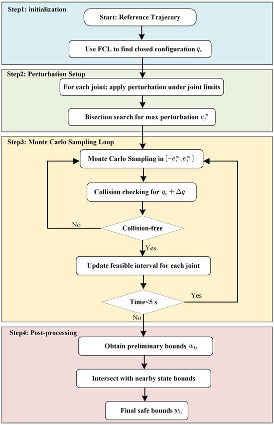
Figure 2. Workflow of the Monte Carlo search strategy.

(1) Identify the robot’s closest configuration $q_c$ to obstacles along the reference trajectory. Using the FCL collision detection library, the reference trajectory is checked to locate the configuration where the manipulator reaches its minimum clearance from surrounding obstacles. This critical configuration serves as the starting point for safe-bound estimation. It should be noted that performing collision checking along the entire trajectory is extremely costly. To balance the accuracy of trajectory representation and computational efficiency, we use only the path nodes generated by the RRT tree as the candidate configurations for collision checking. In addition, during the RRT construction, the collision information at each checked node, namely the minimum distance to obstacles, is stored so that repeated collision checks can be avoided.

(2) Compute the maximum non-colliding perturbation for each individual joint. From configuration ${\mathit{q}}_c$, each joint is independently perturbed within joint limits while ensuring no collision occurs. The largest admissible perturbation for joint j, denoted $e_j^m,j=1,\cdots ,n$, is efficiently obtained using a bisection search. This value represents the collision-free variation range for each joint relative to ${\mathit{q}}_c$.

(3) Conduct Monte Carlo sampling within joint perturbation intervals to determine $w_{1j}$. Using the ranges $[-e_j^m,e_j^m]$, random perturbations are sampled to form perturbation vectors $\Delta \mathit{q}$. Each perturbed configuration ${\mathit{q}}_c+\Delta \mathit{q}$ is collision-checked using FCL. Through repeated sampling and checking, the collision-free perturbation intervals for all joints are estimated. The search runs for a fixed duration of 5 s as default value, leading to the final values of $w_{1j}$.

(4) Improve conservativeness by repeating the search near $q_c$. To enhance robustness, the above procedure may be repeated for two or three configurations in the vicinity of ${\mathit{q}}_c$. The final bounds $w_{1j}$ are obtained by taking the intersection of the corresponding safe perturbation intervals to ensure conservative safety guarantees.

4. Controller Design

To address the aforementioned problem, a state feedback controller has been designed. First, define an error tuning function [44]

$$\alpha \left(t\right)=\left\{\begin{array}{cc}-{\displaystyle \frac{1}{2}}cos\left(\pi {\displaystyle \frac{t}{t_u}}\right)+{\displaystyle \frac{1}{2}},\hfill & t<t_u\hfill \\ 1,\hfill & t\ge t_u\hfill \end{array}\right.$$

(4)

where $t_u>0$ is the design parameter. Through the above function, the error in Equation (2) is modified as

$${\lambda }_{1j}\left(t\right)=\alpha \left(t\right)e_j\left(t\right),j=1,\cdots ,n.$$

(5)

Next, define the virtual control rate

$${\theta }_j\left(t\right)=-a_j{\chi }_j\left(t\right),j=1,\cdots ,n$$

(6)

where $a_j>0$ is the controller parameter, and

$${\chi }_j\left(t\right)=tan\left({\displaystyle \frac{\pi {\lambda }_{1j}\left(t\right)}{2w_{1j}}}\right).$$

(7)

Using Equation (4) for angular velocity transformation, the transformed angular velocity is represented as

$${\lambda }_{2j}\left(t\right)=\alpha \left(t\right){\dot{q}}_j\left(t\right)-{\theta }_j\left(t\right)$$

(8)

and is required to satisfy

$$\left|{\lambda }_{2j}\left(t\right)\right|\le w_{2j},j=1,\cdots ,n$$

(9)

where $w_{2j}$ are positive constants.

Finally, design the control rate as

$$\mathit{\tau }\left(t\right)=-\mathit{c}\mathit{\beta }\left(t\right)\mathit{\delta }\left(t\right)$$

(10)

where $\mathit{c}={\mathrm{diag}}_{i\in j=1,\dots ,n}\left[c_i\right],$ is a diagonal matrix with positive parameters,

$$\mathit{\beta }\left(t\right)=\left[\begin{array}{ccc}{\beta }_1\left(t\right)\hfill & \hfill & \\ \hfill & \ddots \hfill & \\ \hfill & \hfill & {\beta }_n\left(t\right)\hfill \end{array}\right],\mathit{\delta }\left(t\right)=\left[\begin{array}{c}{\delta }_1\left(t\right)\\ ⋮\\ {\delta }_n\left(t\right)\end{array}\right].$$

(11)

Each element of $\mathit{\beta }\left(t\right)$ and $\mathit{\delta }\left(t\right)$ are

$${\beta }_j\left(t\right)={\displaystyle \frac{1}{w_{2j}{cos}^2\left(\frac{\pi {\lambda }_{2j}\left(t\right)}{2w_{2j}}\right)}},j=1,\cdots ,n,$$

(12)

$${\delta }_j\left(t\right)=tan\left({\displaystyle \frac{\pi {\lambda }_{2j}\left(t\right)}{2w_{2j}}}\right),j=1,\cdots ,n.$$

(13)

The parameters $a_j$ and $c_j$ are selected to balance system performance and control effort. Larger values accelerate the convergence of the angular position error ${\lambda }_{1j}$ and angular velocity error ${\lambda }_{2j}$ to their prescribed bounds, but may also increase the control input $\mathit{\tau }$ beyond practical limits. In particular, actuator saturation can cause significant discrepancies between the commanded input $\mathit{\tau }$ and the actual control effort, and may even destabilize the system. Parameter tuning should therefore ensure rapid error attenuation while respecting the constraints imposed by bounded control inputs.

5. Stability Analysis

This section provides the stability analysis of the proposed controller. Before demonstrating the stability of the control system, the following lemma is introduced.

Lemma 2.

If ${\chi }_j\left(t\right)$ and ${\dot{\lambda }}_{1j}\left(t\right)$ are bounded, and $\left|{\lambda }_{1j}\left(t\right)\right|<w_{1j}$ holds, then ${\dot{\theta }}_j\left(t\right)$ keeps bounded.

Proof. 

Differentiating ${\chi }_j\left(t\right)$ with respect to time based on Equation (7) gives

$${\dot{\chi }}_j\left(t\right)={\displaystyle \frac{\pi }{2}}{\displaystyle \frac{1}{{cos}^2\left(\frac{\pi }{2}\frac{{\lambda }_{1j}\left(t\right)}{w_{1j}}\right)}}\left({\displaystyle \frac{{\dot{\lambda }}_{1j}\left(t\right)}{w_{1j}}}\right),j=1,\cdots ,n.$$

(14)

After that, differentiating Equation (6) and then substituting Equation (14) into it yields

$${\dot{\theta }}_j\left(t\right)=-a_j{\displaystyle \frac{\pi }{2}}{S}_j^{-1}\left(t\right)\left({\displaystyle \frac{{\dot{\lambda }}_{1j}\left(t\right)}{w_{1j}}}\right),j=1,\cdots ,n$$

(15)

with

$$S_j^{-1}\left(t\right)={\displaystyle \frac{1}{{cos}^2\left(\frac{\pi }{2}\frac{{\lambda }_{1j}\left(t\right)}{w_{1j}}\right)}}.$$

(16)

Discussing the boundedness of ${\dot{\theta }}_j$ in Equation (15). From Equation (7), it is evident that when ${\chi }_j\left(t\right)$ is bounded and $\left|{\lambda }_{1j}\left(t\right)\right|<w_{1j}$ holds, $S^{-1}\left(t\right)$ in Equation (16) is bounded. Therefore, once ${\chi }_j\left(t\right)$ and ${\dot{\lambda }}_{1j}\left(t\right)$ are bounded, ${\dot{\theta }}_j\left(t\right)$ is also bounded. Therefore, Lemma 2 holds true, and the proof is completed.

Following the above lemmas, we will elaborate on the main results. The statement of the fundamental theorem is as follows. □

Theorem 1.

In the context of the system described in Equation (1), if Assumptions 1–4 are satisfied, then the proposed controller can address Problem 1.

Proof. 

To validate the capability of the proposed controller in addressing Problem 1, it is necessary to demonstrate that the transformed error consistently satisfies

$$\left|{\lambda }_{ij}\left(t\right)\right|<w_{ij},i=1,2,j=1,\dots ,n,t\ge 0.$$

(17)

The validity of the above equation is demonstrated through a proof by contradiction. Assuming that the conditions in Equation (17) are not initially satisfied at the time $t=t_f$, then we obtain

$$\underset{t\to t_f^{-}}{lim}\left|{\lambda }_{ij}\left(t\right)\right|=w_{ij}\left(t_f\right),\exists t_f>0,\exists i\in \{1,2\}.$$

(18)

According to Equations (6)–(8), it can be observed that

$$\left|{\lambda }_{ij}\left(0\right)\right|<w_{ij},i=1,2,j=1,\dots ,n.$$

(19)

Hence, from Equations (18) and (19), we can further derive

$$\left|{\lambda }_{ij}\left(t\right)\right|<w_{ij},i=1,2,j=1,\dots ,n,t<t_f.$$

(20)

Analyzing all errors within the interval $\left[0,t_f\right)$ confirms the validity of Theorem 1. For the sake of conciseness in subsequent analysis, we remove the time parameter t from variables related to time. □

Step 1: For the transformed errors ${\lambda }_{1j},j=1,\cdots ,n$, the following Lyapunov function is constructed

$$V_{1j}={\displaystyle \frac{1}{\pi }}{\chi }_j^2.$$

(21)

Differentiating Equation (21), we obtain

$${\dot{V}}_{1j}={\displaystyle \frac{2}{\pi }}{\chi }_j\dot{{\chi }_j}.$$

(22)

Substituting Equation (14) into Equation (22) yields

$${\dot{V}}_{1j}={\displaystyle \frac{1}{w_{1j}}}{\chi }_j{\displaystyle \frac{1}{{cos}^2\left(\frac{\pi }{2}\frac{{\lambda }_{1j}}{w_{1j}}\right)}}{\dot{\lambda }}_{1j}.$$

(23)

Continuing with the calculation for ${\dot{\lambda }}_{1j}$, we derive the derivative of ${\lambda }_{1j}$ from Equation (5) to obtain

$${\dot{\lambda }}_{1j}=\dot{\alpha }\left(q_j-q_{dj}\right)+\alpha {\dot{q}}_j-\alpha {\dot{q}}_{dj},j=1,\cdots ,n.$$

(24)

Substituting Equations (6) and (8) into Equation (24) gives

$${\dot{\lambda }}_{1j}=\dot{\alpha }\left(q_j-q_{dj}\right)-\alpha {\dot{q}}_{dj}+{\lambda }_{2j}-a_j{\chi }_j.$$

(25)

Next, substituting Equation (25) into Equation (23), one has

$${\dot{V}}_{1j}={\displaystyle \frac{1}{w_{1j}}}{\chi }_j{\displaystyle \frac{1}{{cos}^2\left(\frac{\pi }{2}\frac{{\lambda }_{1j}}{w_{1j}}\right)}}\left(I_{1j}-a_j{\chi }_j\right)$$

(26)

where

$$I_{1j}=\dot{\alpha }\left(q_j-q_{dj}\right)-\alpha {\dot{q}}_{dj}+{\lambda }_{2j}.$$

(27)

Now, let’s discuss the boundedness of $I_{1j}$ within the range $t<t_f$. (1) From Equation (4), it is evident that both $\alpha$ and $\dot{\alpha }$ are bounded; (2) According to Assumption 1, $q_j$ is bounded, and Assumption 4 states that $q_{dj}$ and ${\dot{q}}_{dj}$ are bounded. Therefore, $\dot{\alpha }\left(q_j-q_{dj}\right)$ and $\alpha {\dot{q}}_{dj}$ are bounded. (3) Within the range $t<t_f$, ${\chi }_j$ is bounded, and we can infer that ${\lambda }_{2j}$ is bounded from Equation (8).

Based on the above discussion and by the closure property of bounded sets under finite summation, it is obvious that $I_{1j}$ is bounded. Therefore, there exists a positive constant ${\overline{I}}_{1j}$ that satisfies the following inequality

$$\left|I_{1j}\right|<{\overline{I}}_{1j},t<t_f.$$

(28)

Injecting Equation (28) into Equation (26) gives

$${\dot{V}}_{1j}\le {\displaystyle \frac{1}{w_{1j}}}{\displaystyle \frac{1}{{cos}^2\left(\frac{\pi }{2}\frac{{\lambda }_{1j}}{w_{1j}}\right)}}\left|{\chi }_j\right|\left({\overline{I}}_{1j}-a_j\left|{\chi }_j\right|\right).$$

(29)

In Equation (29), it can be observed that in order to ensure ${\dot{V}}_{1j}<0$ within the interval $\left[0,t_f\right)$, the following condition holds

$$\left|{\chi }_j\right|>{\displaystyle \frac{{\overline{I}}_{1j}}{a_j}},j=1,\cdots ,n.$$

(30)

On the other hand, it should be noted that when $t=0$, according to Equation (5), we have ${\lambda }_{1j}\left(0\right)=0$, which implies ${\chi }_j\left(0\right)=0$. Therefore, within the interval $\left[0,t_f\right)$, there exists

$$\left|{\chi }_j\right|\le {\displaystyle \frac{{\overline{I}}_{1j}}{a_j}},j=1,\cdots ,n.$$

(31)

As evident from the contradiction between Equations (30) and (31), it can be inferred that ${\lambda }_{1j}$ does not tend to $w_{1j},j=1,\cdots ,n$. In other words, there always exists a positive constant ${\Delta }_{1j}>0$ such that

$$\left|{\lambda }_{1j}\right|<w_{1j}-{\Delta }_{1j}<w_{1j},j=1,\cdots ,n,t<t_f.$$

(32)

Step 2: For the transformed errors ${\lambda }_{2j},j=1,\cdots ,n$, the following Lyapunov function is constructed

$${\mathit{V}}_2\left(t\right)={\displaystyle \frac{1}{\pi }}{\mathit{\delta }}^{\mathrm{T}}\left(t\right)\mathit{\delta }\left(t\right).$$

(33)

Differentiating Equation (33) yields

$${\dot{\mathit{V}}}_2\left(t\right)={\displaystyle \frac{2}{\pi }}{\mathit{\delta }}^{\mathrm{T}}\left(t\right)\dot{\mathit{\delta }}\left(t\right).$$

(34)

Each element of $\dot{\delta }\left(t\right)$ is calculated by differentiating Equation (13)

$${\dot{\delta }}_j={\displaystyle \frac{\pi }{2}}{\beta }_j{\dot{\lambda }}_{2j}$$

(35)

where ${\dot{\lambda }}_{2j}$ is obtained by differentiating ${\lambda }_{2j}$ from Equation (8)

$${\dot{\lambda }}_{2j}=\dot{\alpha }{\dot{q}}_j+\alpha {\ddot{q}}_j-{\dot{\theta }}_j.$$

(36)

Finally, substituting Equation (36) into Equation (35) produces

$${\dot{\delta }}_j={\displaystyle \frac{\pi }{2}}{\beta }_j\left(\dot{\alpha }{\dot{q}}_j+\alpha {\ddot{q}}_j-{\dot{\theta }}_j\right).$$

(37)

Define the following vectors and matrix

$$\begin{array}{cc}\hfill & {\mathit{\lambda }}_2\left(t\right)={\left[{\lambda }_{21},\cdots ,{\lambda }_{2n}\right]}^{\mathrm{T}},\hfill \\ \hfill & \mathit{\theta }\left(t\right)={\left[{\theta }_1,\cdots ,{\theta }_n\right]}^{\mathrm{T}},\hfill \\ \hfill & {\mathit{w}}_2=diag\left[{\mathrm{w}}_{21},\cdots ,{\mathrm{w}}_{2n}\right]\hfill \end{array}$$

(38)

Based on Equations (11) and (38), we transform Equation (37) into the following vector

$$\dot{\mathit{\delta }}={\displaystyle \frac{\pi }{2}}\mathit{\beta }\left(\dot{\alpha }\dot{\mathit{q}}+\alpha \ddot{\mathit{q}}-\dot{\mathit{\theta }}\right).$$

(39)

Substituting Equation (39) into Equation (34) generates

$${\dot{\mathit{V}}}_2={\mathit{\delta }}^{\mathrm{T}}\mathit{\beta }\left(\dot{\alpha }\dot{\mathit{q}}+\alpha \ddot{\mathit{q}}-\dot{\mathit{\theta }}\right).$$

(40)

Based on Equation (1), it can be obtained that

$$\ddot{\mathit{q}}=\mathit{H}\mathit{\tau }-\mathit{Hh}$$

(41)

where

$$\mathit{H}={\mathit{M}}^{-1}\left(\mathit{q}\right),$$

$$\mathit{h}=\mathit{C}(\mathit{q},\dot{\mathit{q}})\dot{\mathit{q}}\left(t\right)+\mathit{N}(\mathit{q},\dot{\mathit{q}})+\mathit{D}\left(t\right).$$

Inserting Equation (41) into Equation (40) yields

$${\dot{\mathit{V}}}_2={\mathit{\delta }}^{\mathrm{T}}\mathit{\beta }\left({\mathit{I}}_2+\alpha \mathit{H}\mathit{\tau }\right)$$

(42)

where

$${\mathit{I}}_2=\dot{\alpha }\dot{\mathit{q}}-\dot{\mathit{\theta }}-\alpha \mathit{Hh}.$$

(43)

Discussing the boundedness of ${\mathit{I}}_2$ within the interval $\left[0,t_f\right)$. (1) Based on Equation (4), it is evident that $\dot{\alpha }$ is bounded. Simultaneously, the sensed angular velocities $\dot{\mathit{q}}$ are bounded, hence $\dot{\alpha }\dot{\mathit{q}}$ is bounded; (2) According to Lemma 2, $\dot{\mathit{\theta }}$ is bounded; (3) As shown in Lemma 1, $\mathit{H}$ is bounded. Based on Assumptions 1 to 3, $\mathit{h}$ is also bounded. Therefore, $\alpha \mathit{Hh}$ is bounded.

Given the discussion above, it is clear that ${\mathit{I}}_2$ is bounded within the interval $[0,t_f)$, and there exists a positive constant ${\overline{I}}_2$ satisfying

$$∥{\mathit{I}}_2∥<{\overline{I}}_2,t<t_f.$$

(44)

Furthermore, according to Lemma 1, there exist two positive constants $\underline{m}$ and $\overline{m}$ satisfying

$$\underline{m}{\parallel \mathit{q}\parallel }^2\le {\mathit{q}}^{\mathrm{T}}{\mathit{M}}^{-1}\mathit{q}\le \overline{m}{\parallel \mathit{q}\parallel }^2.$$

(45)

Introducing the control law from Equation (10) into Equation (42), we obtain

$${\dot{\mathit{V}}}_2={\mathit{\delta }}^{\mathrm{T}}\mathit{\beta }{\mathit{I}}_2-c\alpha {\mathit{\delta }}^{\mathrm{T}}\mathit{\beta }\mathit{H}\mathit{\beta }\mathit{\delta }.$$

(46)

Then, substituting Equations (44) and (45) into Equation (46), we get the follow- ing inequality

$${\dot{\mathit{V}}}_2\le \parallel \mathit{\beta }\mathit{\delta }\parallel \left({\overline{I}}_2-c\alpha \underline{m}\parallel \mathit{\beta }\mathit{\delta }\parallel \right),t<t_f.$$

(47)

To make ${\dot{\mathit{V}}}_2<0$, it should hold

$$\alpha \parallel \mathit{\beta }\mathit{\delta }\parallel >{\displaystyle \frac{{\overline{I}}_2}{c\underline{m}}}.$$

(48)

When Equation (17) is not satisfied, Equation (18) holds. According to Equations (11)–(13), it can been seen that

$$\underset{t\to t_f^{-}}{lim}\alpha \parallel \mathit{\beta }\mathit{\delta }\parallel =\infty .$$

(49)

From Equation (8), it is evident that ${\lambda }_{2j}\left(0\right)=0$. Substituting this result into Equation (12) yields ${\beta }_j\left(0\right)=w_{2j}^{-1}$, and inserting it into Equation (13) gives ${\delta }_j\left(0\right)=0$. Therefore, we have

$$\alpha \left(0\right)\parallel \mathit{\beta }\left(0\right)\mathit{\delta }\left(0\right)\parallel =0.$$

(50)

According to Equations (49) and (50), along with the continuity of $\alpha \left|\mathit{\beta }\mathit{\delta }\right|$, it can be deduced that

$$\alpha \parallel \mathit{\beta }\mathit{\delta }\parallel <{\displaystyle \frac{{\overline{I}}_2}{c\underline{m}}},\exists 0<t_r<t_f.$$

(51)

Therefore, from the contradictory results of Equations (48) and (51), it can be concluded that ${\lambda }_{2j}$ will not approach $w_{2j},j=1,\cdots ,n$, and there always exists ${\Delta }_{2j}>0$ such that

$$\left|{\lambda }_{2j}\right|<w_{2j}-{\Delta }_{2j}<w_{2j},j=1,\cdots ,n,t<t_f.$$

(52)

Combine Equation (32) from step 1 with Equation (52) from step 2, and take into account the continuity of ${\lambda }_{ij}$, the following result is obtained that

$$\underset{t\to t_f}{lim}\left|{\lambda }_{ij}\left(t\right)\right|\le w_{ij}-{\Delta }_{ij}<w_{ij},i=1,2,t<t_f.$$

(53)

As the result of Equation (53) contradicts the assumption in Equation (18), the assumption is not valid. Therefore, $|{\lambda }_{ij}|,j=1,2,j=1,\cdots ,n$ will not approach the predefined errors $w_{ij}$ throughout the entire range of $t>0$.

Step 3: Following the conclusions drawn from the analyses in steps 1 and 2, we delve into the boundedness of other signals within the closed-loop system. These findings affirm that the outcomes detailed in Equations (7), (12) and (13) are bounded. Additionally, when examining Equations (8) and (17), it becomes evident that velocities are bounded. Furthermore, both ${\theta }_j$ in Equation (6) and $\mathit{\tau }$ in Equation (10) exhibit bounded characteristics. As a result, we can assert that all signals within the closed-loop system maintain boundedness. This marks the successful validation of Theorem 1.

6. Experiments and Results

6.1. Experimental Setups

To validate the effectiveness of the proposed controller, the Baxter (Rethink Robotics Inc., Boston, MA, USA), bimanual robotic manipulators, is employed as the controlled object. Each manipulator consists of seven degrees of freedom, and each joint is equipped with a Series Elastic Actuator (SEA) to provide flexibility for the manipulator, along with an encoder to measure the joint’s angular position and velocity. The joint configuration of the Baxter robotic manipulator closely resembles that of a human arm, comprising two shoulder joints (S0 and S1), two elbow joints (E0 and E1), and three wrist joints (W0, W1, and W2), as illustrated in Figure 3. The motion range and maximum velocity of each joint are presented in Table 1. To assess the controller’s performance, the trajectory tracking experiments for three distinct scenarios are considered.

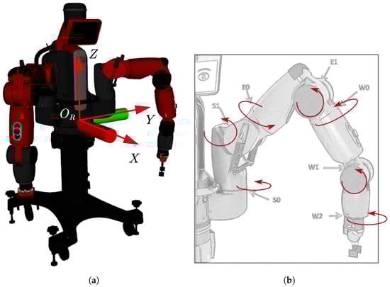
Figure 3. Baxter robot. (a) Baxter dual-arm robot; (b) Baxter arm joints.

Table 1. Joint motion range and maximum velocity of each joint of the Baxter robotic manipulator.

Joint	Min. Pos. (rad)	Max. Pos. (rad)	Max. Vel. (rad/s)
S0	−1.7016	1.7016	3.5
S1	−2.147	1.047	3.5
E0	−3.0541	3.0541	3.5
E1	−0.05	2.618	3.5
W0	−3.059	3.059	4.0
W1	−1.5707	2.094	4.0
W2	−3.059	3.059	4.0

6.2. Experimental Results

Case 1: Track sinusoidal trajectories in free space. This scenario validates the proposed controller’s ability to achieve trajectory tracking for each joint within a specified error bound. The right arm of the robotic manipulator operates in a obstacle-free environment, with the reference trajectories of all joints following sinusoidal curves. The initial configuration of the right arm is set to $q_{\mathrm{init}}={[-0.27,1.05,-0.001,0.49,-0.08,-0.06,0.03]}^{\mathrm{T}}$ rad, and the duration of all joint trajectories is 10 s. The reference trajectory and controller parameters for each joint are presented in Table 2. After executing the trajectory, the robotic manipulator returns to the initial configuration.

Table 2. Reference trajectory and controller parameters of each joint.

Joint	${\mathit{w}}_{1\mathit{j}}$	${\mathit{w}}_{2\mathit{j}}$	${\mathit{a}}_{\mathit{j}}$	${\mathit{c}}_{\mathit{j}}$	Joint Trajectories
S0	0.05	3	15	35	$sin\left({\displaystyle \frac{\pi t}{5}}\right)-0.27$
S1	0.05	3.5	15	35	$-1.5sin\left({\displaystyle \frac{\pi t}{10}}\right)+1.05$
E0	0.05	3.5	15	35	$-1.5sin\left({\displaystyle \frac{\pi t}{5}}\right)-0.001$
E1	0.05	3.5	10	30	$0.3sin\left({\displaystyle \frac{\pi t}{5}}\right)+0.49$
W0	0.075	3.5	10	30	$-1.5sin\left({\displaystyle \frac{\pi t}{5}}\right)-0.08$
W1	0.05	3.5	15	30	$1.4sin\left({\displaystyle \frac{\pi t}{5}}\right)-0.06$
W2	0.075	3.5	10	15	$1.7sin\left({\displaystyle \frac{\pi t}{5}}\right)+0.03$

The controller parameters listed in the table above are applied to each joint, and the tracking results of the reference trajectories are depicted in Figure 4. Upon completion of the run, the robotic manipulator returns to its initial configuration, as shown in Figure 4a. Figure 4b demonstrates that the designed controllers have successfully achieved angular position tracking for each joint. Simultaneously, the trajectory tracking error for each joint is illustrated in Figure 5. It can be observed from these figures that the angular position tracking errors $e_j$ for all joints remain within the specified error bounds of $(-w_{1j},w_{1j}),j=1,\dots ,7$, which serves as a prerequisite for ensuring the safe motion of the robotic arm in confined spaces.

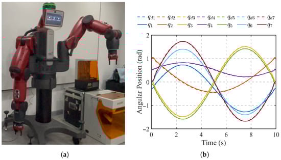
Figure 4. Case 1: Sinusoidal trajectory tracking in the right arm’s free space. (a) Initial configuration; (b) Tracking results.

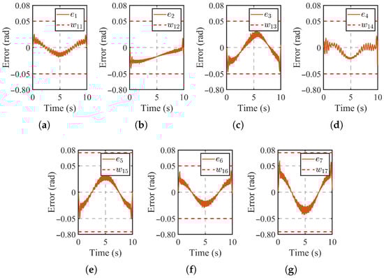
Figure 5. Case 1: Tracking errors of sinusoidal trajectories from joint $\mathrm{S}0$ to $\mathrm{W}2$.

Case 2: Collision-free trajectory tracking. In this scenario, we investigate trajectory tracking within confined spaces. Initially, a constrained bookshelf environment is established, as illustrated in Figure 6, with the robotic manipulator’s initial and target configurations depicted in Figure 6a and Figure 6b, respectively. For this environment, obstacle perception is achieved using a Kinect camera calibration in an eye-to-hand way, and then environmental point clouds are converted into octrees for planning tasks [45]. Subsequently, a sampling-based motion planning algorithm [7] is utilized to generate collision-free and smooth joint trajectories, as shown in Figure 6c. The manipulator is required to transition between layers of the constrained bookshelf. The red trajectory at the end-effector is obtained through forward kinematics calculation based on the planned joint trajectory.

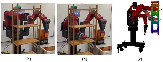
Figure 6. Case 2: Collision-free trajectory tracking in confined spaces. (a) Initial configuration; (b) Goal configuration; (c) Planned collision-free trajectory in workspace.

The proposed PPC controller is utilized to track the joint trajectories planned in this scenario, focusing solely on the tracking results for joints $\mathrm{S}0$ and $\mathrm{E}0$ for conciseness. Unless explicitly stated otherwise, all subsequent experiments adhere to the same trajectory tracking requirements. Controller parameters for the two joints are specified as $w_{11}=0.033$, $w_{21}=2.5$, $a_1=10$, $c_1=37$ and $w_{13}=0.024$, $w_{23}=2.5$, $a_3=10$, $c_3=30$. In our experiments, we chose PID and Yiannis’s PPC [25] controllers for comparison, as both are model-free controllers characterized by simple structures and have been validated on real robotic platforms. The two controlles are employed to track identical reference trajectories with PID controller parameters $P_1=700$, $I_1=0.01$, $D_1=0.01$ and $P_3=4500$, $I_3=35$, $D_3=1$, and Yiannis’s PPC controller parameters $K_{q1}=0.1$, $K_{y1}=0.1$, $K_{q3}=0.5$, and $K_{y3}=0.4$. The angular position error bounds are assigned the same value as in our controller, with ${\rho }_{q\infty 1}=0.033$ and ${\rho }_{q\infty 3}=0.024$, while the angular velocity error bounds are assigned with ${\rho }_{y\infty 1}=0.5$ and ${\rho }_{y\infty 3}=0.3$.

Figure 7 illustrates the tracking outcomes obtained with the proposed PPC controller. In Figure 7a, we observe the angular position tracking for joints S0 and E0 utilizing the proposed controller. As demonstrated in Figure 7b,c, the angular tracking errors of the two joints consistently adhere to the predetermined safe error bounds. Consequently, the robotic manipulator adeptly accomplishes trajectory tracking within the confined space without safety concerns. In Figure 8a, we observe the results of trajectory tracking using the PID controller. While this controller effectively achieves trajectory tracking, it lacks the capability to accurately anticipate tracking performance beforehand. Notably, the angular tracking errors for joints S0 and E0 exceed the specified safety error bounds in Figure 8b,c, indicating potential collision risks. In contrast to the PID controller, the proposed controller ensures that angular position tracking errors for all joints of the robotic manipulator consistently remain within safe error bounds, thereby ensuring the safety of trajectory tracking. As illustrated in Figure 9, the tracking results of Yiannis’s PPC controller for joints S0 and E0 exhibit a performance that is both similar to and comparable with that of our controller, with all joint errors remaining within the defined safety error bounds. The tracking errors of the three controllers, quantified using the root mean square tracking error (RMSTE) metric and summarized in Table 3, show that the accuracy of the proposed PPC controller is comparable to that of Yiannis’s PPC controller.

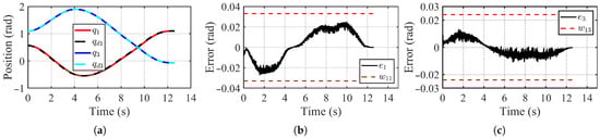
Figure 7. Case 2: Experiment results of joints S0 and E0 using the proposed PPC controller. (a) Angular position tracking. (b) Angular position tracking error of joint S0; (c) Angular position tracking error of joint E0.

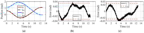
Figure 8. Case 2: Experiment results of joints S0 and E0 using the PID controller. (a) Angular position tracking. (b) Angular position tracking error of joint S0; (c) Angular position tracking error of joint E0.

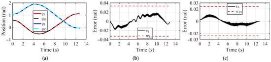
Figure 9. Case 2: Experiment results of joints S0 and E0 using the Yiannis’s PPC controller [25]. (a) Angular position tracking. (b) Angular position tracking error of joint S0; (c) Angular position tracking error of joint E0.

Table 3. RMSTE of different controllers in Case 2.

Joint	Proposed PPC	PID	Yiannis’s PPC
S0	0.0149	0.0202	0.0104
E0	0.0053	0.0151	0.0052

When the robotic manipulator tracks the reference trajectory using the proposed controller, Figure 10 illustrates the state of the manipulator at certain time steps, indicating its successful avoidance of collisions with the bookshelf during motion. From Figure 10d, it can be observed that, the manipulator adopts a configuration where both the upper and lower arms retract backward and fold to navigate through the confined space.

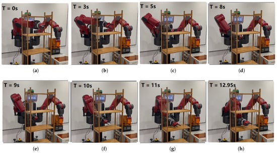
Figure 10. Robot’s state at certain time steps during the trajectory execution process using the proposed controller.

Case 3: Collision-free trajectory tracking with load. In this scenario, the manipulator continues to follow the previously defined reference trajectory, and a 1.8 kg payload is applied at the end-effector to simulate external disturbance, as illustrated in Figure 11. It is worth noting that the Baxter manipulator is designed to withstand a maximum payload of 2.2 kg at the wrist.

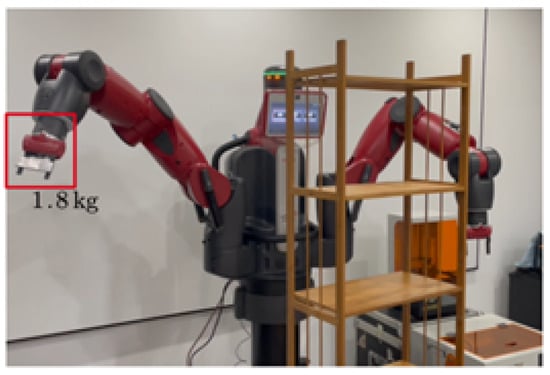
Figure 11. Case 3: Trajectory tracking with end-effector load.

Initially, we attempted to keep all the control parameters unchanged, and it was observed that both the proposed controller and the PID controller continued to achieve tracking of the reference trajectory. The joint tracking errors for both controllers are depicted in Figure 12a,b. However, the proposed controller outperforms the PID controller in terms of tracking accuracy (see Table 4). With the designed PPC controller, the joint tracking errors consistently stay within the predefined bounds, as observed previously. When guided by the proposed controller, the manipulator smoothly follows the reference trajectory without any collisions with the surrounding objects. Conversely, when utilizing the PID controller, the joint tracking errors exhibit noticeable fluctuations, exceeding the predetermined safety thresholds. As a result, this results in instances where the manipulator, under PID control, brushes against the bookshelf, as illustrated in Figure 13.

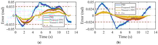
Figure 12. Case 3: Experiment results of joint S0 and E0 using the proposed controller, PID controller and Yiannis’s PPC controller [25] with 1.8 kg load at the end-effector. (a) Tracking errors of joint S0 using the two controllers; (b) Tracking errors of joint E0 using the two controllers.

Table 4. RMSTE of different controllers in Case 3.

Joint	Proposed PPC	PID	Yiannis’s PPC
S0	0.0169	0.0284	0.0093
E0	0.0100	0.0259	0.0065

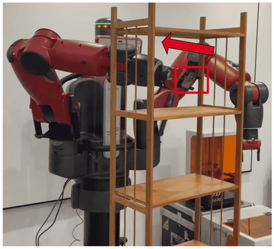
Figure 13. Case 3: Local contact with the bookshelf during trajectory execution using the PID controller.

Figure 12a,b indicate that the variation in joint tracking errors is more gradual with the designed controller, whereas the PID controller’s tracking errors oscillate due to external load disturbances. Remarkably, even when faced with unpredictable external disruptions, the proposed controller maintains joint trajectory tracking errors within the specified bounds, ensuring safety in confined environments. Furthermore, the proposed controller’s structure eliminates the need for additional adaptive techniques, such as neural networks or fuzzy systems, simplifying the compensation for unknown disturbances.

When using the original control parameters, Yiannis’s PPC controller was unable to complete the trajectory tracking task. Once the position error of any joint exceeded the system-defined safety limit, for example 0.9 rad for the Baxter right E0 joint, the robot automatically halted command execution through its safety mechanism. This made it necessary to readjust the controller parameters.

This difficulty arises because Yiannis’s PPC controller relies directly on joint velocity error bounds. These bounds are highly sensitive to measurement noise and external disturbances. Even small fluctuations in joint velocity can cause the velocity errors to exceed their required limits, which then leads to position errors moving beyond their admissible range. Several unsuccessful attempts to adjust the parameters, as shown in Figure 14 and Figure 15, further confirm this sensitivity and illustrate the challenges of stabilizing the controller under changes in external loading.

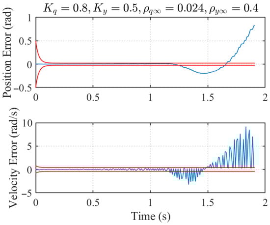
Figure 14. Situation 1: Joint position and velocity errors under unsuccessful parameter-tuning attempt.

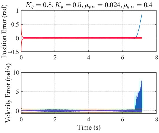
Figure 15. Situation 2: Joint position and velocity errors under unsuccessful parameter-tuning attempt.

To achieve safe operation under these conditions, the velocity error bounds and the associated gains required careful and repeated tuning. After a considerable amount of trial-and-error adjustments, the PPC parameters were finally set to $K_{q1}=0.3,$ $K_{y1}=0.5,$ $K_{q3}=0.7,K_{y3}=0.7,{\rho }_{y\infty 1}=0.7,{\rho }_{y\infty 3}=0.7,$ which allowed the robot to complete the safe trajectory tracking task.

In contrast, the proposed controller does not depend on velocity-error feedback. This feature gives it much stronger robustness to noise and significantly reduces the demand for parameter tuning. The controller maintains stable and reliable tracking performance without any retuning, even when the external load changes. As shown in Figure 12a,b together with Table 4, the tracking accuracy of the proposed controller remains comparable to that of Yiannis’s PPC controller while offering much better robustness and practical usability.

7. Conclusions

In spatially constrained environments with obstacles, robotic manipulators face inherent risks of collision during trajectory execution. This paper addresses the problem of constraining joint tracking errors and introduces a controller with a straightforward structure that ensures each joint’s tracking error consistently remains within predefined safe bounds. This control strategy enables safe execution along a reference trajectory even under model uncertainties and unknown external disturbances. To determine safe error bounds for joint trajectory tracking, we propose a Monte Carlo–based search strategy. The controller further demonstrates robustness to external disturbances, owing to its intrinsic tuning function and error transformation techniques. Importantly, it does not rely on velocity-error feedback, making its gains easy to tune and less sensitive to noise, which significantly enhances its practical usability on real robotic systems. The effectiveness and practicality of the proposed controller are validated through trajectory tracking experiments on the Baxter robot across multiple scenarios, confirming its suitability and reliability for real-world applications requiring safe and robust manipulation.

One evident limitation of the proposed controller is that the joint error bounds are constant, primarily for the sake of simplification, given the complexity of searching for collision-free bounds in high-dimensional joint spaces. In future work, designing efficient search algorithms to determine joint error bounds that adapt in real time to spatial constraints will greatly broaden the applicability of the current controller (e.g., in environments with dense obstacles or narrow pipelines). Nevertheless, integrating obstacle-avoidance motion planning algorithms with the error bounds of PPC could provide new insights and advancements for ensuring safe robotic operations.

References

- Lee, M.; Lee, J.; Lee, D. Narrow Passage Path Planning Using Collision Constraint Interpolation. In Proceedings of the 2025 IEEE International Conference on Robotics and Automation (ICRA), Atlanta, GA, USA, 17–23 May 2025; IEEE: Piscataway, NJ, USA, 2025; pp. 1–7. [Google Scholar]
- Orthey, A.; Toussaint, M. Section patterns: Efficiently solving narrow passage problems in multilevel motion planning. IEEE Trans. Robot. 2021, 37, 1891–1905. [Google Scholar] [CrossRef]
- Nubert, J.; Köhler, J.; Berenz, V.; Allgöwer, F.; Trimpe, S. Safe and fast tracking on a robot manipulator: Robust mpc and neural network control. IEEE Robot. Autom. Lett. 2020, 5, 3050–3057. [Google Scholar] [CrossRef]
- Dai, L.; Yu, Y.; Zhai, D.; Huang, T.; Xia, Y. Robust model predictive tracking control for robot manipulators with disturbances. IEEE Trans. Ind. Electron. 2020, 68, 4288–4297. [Google Scholar] [CrossRef]
- Zhang, M.; Gosselin, C. Optimal design of safe planar manipulators using passive torque limiters. J. Mech. Robot. 2016, 8, 011008. [Google Scholar] [CrossRef]
- Batkovic, I.; Ali, M.; Falcone, P.; Zanon, M. Safe trajectory tracking in uncertain environments. IEEE Trans. Autom. Control 2022, 68, 4204–4217. [Google Scholar] [CrossRef]
- Orthey, A.; Chamzas, C.; Kavraki, L.E. Sampling-based motion planning: A comparative review. Annu. Rev. Control. Robot. Auton. Syst. 2023, 7, 285–310. [Google Scholar] [CrossRef]
- Muhammed, M.L.; Flaieh, E.H.; Humaidi, A.J. Embedded system design of path planning for planar manipulator based on chaos A* algorithm with known-obstacle environment. J. Eng. Sci. Technol. 2022, 17, 4047–4064. [Google Scholar]
- Lippi, M.; Marino, A. Human multi-robot safe interaction: A trajectory scaling approach based on safety assessment. IEEE Trans. Control Syst. Technol. 2020, 29, 1565–1580. [Google Scholar] [CrossRef]
- Chen, M.; Wang, H.; Liu, X. Fuzzy adaptive fixed-time quantized feedback control for a class of nonlinear systems. Acta Autom. Sin. 2021, 47, 2823–2830. [Google Scholar]
- Wang, H.; Xu, K.; Zhang, H. Adaptive finite-time tracking control of nonlinear systems with dynamics uncertainties. IEEE Trans. Autom. Control 2022, 68, 5737–5744. [Google Scholar] [CrossRef]
- Xu, K.; Wang, H.; Liu, P.X. Singularity-free adaptive fixed-time tracking control for MIMO nonlinear systems with dynamic uncertainties. IEEE Trans. Circuits Syst. Part II Express Briefs 2023, 71, 1356–1360. [Google Scholar] [CrossRef]
- Cruz-Ortiz, D.; Chairez, I.; Poznyak, A. Sliding-mode control of full-state constraint nonlinear systems: A barrier lyapunov function approach. IEEE Trans. Syst. Man Cybern. Syst. 2022, 52, 6593–6606. [Google Scholar] [CrossRef]
- Bu, X. Prescribed performance control approaches, applications and challenges: A comprehensive survey. Asian J. Control 2023, 25, 241–261. [Google Scholar] [CrossRef]
- Li, B.; Wen, S.; Yan, Z.; Wen, G.; Huang, T. A survey on the control lyapunov function and control barrier function for nonlinear-affine control systems. IEEE/CAA J. Autom. Sin. 2023, 10, 584–602. [Google Scholar] [CrossRef]
- Lewis, F.L.; Dawson, D.M.; Abdallah, C.T. Robot Manipulator Control: Theory and Practice; CRC Press: Boca Raton, FL, USA, 2003. [Google Scholar]
- Yang, C.; Huang, D.; He, W.; Cheng, L. Neural control of robot manipulators with trajectory tracking constraints and input saturation. IEEE Trans. Neural Netw. Learn. Syst. 2020, 32, 4231–4242. [Google Scholar] [CrossRef]
- Jahanshahi, H.; Yao, Q.; Khan, M.I.; Moroz, I. Unified neural output-constrained control for space manipulator using tan-type barrier Lyapunov function. Adv. Space Res. 2023, 71, 3712–3722. [Google Scholar] [CrossRef]
- Alhajeri, M.S.; Abdullah, F.; Christofides, P.D. Control Lyapunov barrier function-based predictive control of nonlinear systems using physics-informed recurrent neural networks. Chem. Eng. Sci. 2025, 321, 122695. [Google Scholar] [CrossRef]
- Li, C.; Liu, F.; Wang, Y.; Buss, M. Concurrent learning-based adaptive control of an uncertain robot manipulator with guaranteed safety and performance. IEEE Trans. Syst. Man Cybern. Syst. 2021, 52, 3299–3313. [Google Scholar] [CrossRef]
- Bechlioulis, C.P.; Rovithakis, G.A. Robust adaptive control of feedback linearizable MIMO nonlinear systems with prescribed performance. IEEE Trans. Autom. Control 2008, 53, 2090–2099. [Google Scholar] [CrossRef]
- Shi, W. Adaptive fuzzy output-feedback control for nonaffine MIMO nonlinear systems with prescribed performance. IEEE Trans. Fuzzy Syst. 2020, 29, 1107–1120. [Google Scholar] [CrossRef]
- Wang, M.; Yang, A. Dynamic learning from adaptive neural control of robot manipulators with prescribed performance. IEEE Trans. Syst. Man Cybern. Syst. 2017, 47, 2244–2255. [Google Scholar] [CrossRef]
- Sun, Y.; Liu, J.; Gao, Y.; Liu, Z.; Zhao, Y. Adaptive neural tracking control for manipulators with prescribed performance under input saturation. IEEE/ASME Trans. Mechatronics 2022, 28, 1037–1046. [Google Scholar] [CrossRef]
- Karayiannidis, Y.; Papageorgiou, D.; Doulgeri, Z. A model-free controller for guaranteed prescribed performance tracking of both robot joint positions and velocities. IEEE Robot. Autom. Lett. 2016, 1, 267–273. [Google Scholar] [CrossRef]
- Liang, J.; Chen, Y.; Lai, N.; He, B.; Miao, Z.; Wang, Y. Low-complexity prescribed performance control for unmanned aerial manipulator robot system under model uncertainty and unknown disturbances. IEEE Trans. Ind. Inf. 2021, 18, 4632–4641. [Google Scholar] [CrossRef]
- Wei, C.; Chen, Q.; Liu, J.; Yin, Z.; Luo, J. An overview of prescribed performance control and its application to spacecraft attitude system. Proc. Inst. Mech. Eng. Part I J. Syst. Control Eng. 2021, 235, 435–447. [Google Scholar] [CrossRef]
- Gao, X.; Li, X.; Sun, Y.; Hao, L.; Yang, H.; Xiang, C. Model-free tracking control of continuum manipulators with global stability and assigned accuracy. IEEE Trans. Syst. Man Cybern. Syst. 2020, 52, 1345–1355. [Google Scholar] [CrossRef]
- Humaidi, A.J.; Abdulkareem, A.I. Design of Augmented Nonlinear PD Controller of Delta/Par4-Like Robot. J. Control Sci. Eng. 2019, 2019, 7689673. [Google Scholar] [CrossRef]
- Xu, Z.; Xie, N.; Shen, H.; Hu, X.; Liu, Q. Extended state observer-based adaptive prescribed performance control for a class of nonlinear systems with full-state constraints and uncertainties. Nonlinear Dyn. 2021, 105, 345–358. [Google Scholar] [CrossRef]
- Ma, H.; Zhou, Q.; Li, H.; Lu, R. Adaptive prescribed performance control of a flexible-joint robotic manipulator with dynamic uncertainties. IEEE Trans. Cybern. 2021, 52, 12905–12915. [Google Scholar] [CrossRef]
- Sui, S.; Chen, C.P.; Tong, S. A novel adaptive NN prescribed performance control for stochastic nonlinear systems. IEEE Trans. Neural Netw. Learn. Syst. 2020, 32, 3196–3205. [Google Scholar] [CrossRef]
- Liang, J.; Chen, Y.; Wu, Y.; Miao, Z.; Zhang, H.; Wang, Y. Adaptive prescribed performance control of unmanned aerial manipulator with disturbances. IEEE Trans. Autom. Sci. Eng. 2022, 20, 1804–1814. [Google Scholar] [CrossRef]
- El-Ferik, S.; Hashim, H.A.; Lewis, F.L. Neuro-adaptive distributed control with prescribed performance for the synchronization of unknown nonlinear networked systems. IEEE Trans. Syst. Man Cybern. Syst. 2017, 48, 2135–2144. [Google Scholar] [CrossRef]
- Ni, J.; Ahn, C.K.; Liu, L.; Liu, C. Prescribed performance fixed-time recurrent neural network control for uncertain nonlinear systems. Neurocomputing 2019, 363, 351–365. [Google Scholar] [CrossRef]
- Zerari, N.; Chemachema, M. Robust adaptive neural network prescribed performance control for uncertain CSTR system with input nonlinearities and external disturbance. Neural Comput. Appl. 2020, 32, 10541–10554. [Google Scholar] [CrossRef]
- Li, K.; Li, Y. Fuzzy adaptive optimization prescribed performance control for nonlinear vehicle platoon. IEEE Trans. Fuzzy Syst. 2023, 32, 360–372. [Google Scholar] [CrossRef]
- Cui, G.; Yu, J.; Shi, P. Observer-based finite-time adaptive fuzzy control with prescribed performance for nonstrict-feedback nonlinear systems. IEEE Trans. Fuzzy Syst. 2020, 30, 767–778. [Google Scholar] [CrossRef]
- Murray, R.M.; Li, Z.; Sastry, S.S. A Mathematical Introduction to Robotic Manipulation; CRC Press: Boca Raton, FL, USA, 2017. [Google Scholar]
- Zhang, J.X.; Yang, G.H. Fault-tolerant output-constrained control of unknown Euler–Lagrange systems with prescribed tracking accuracy. Automatica 2020, 111, 108606. [Google Scholar] [CrossRef]
- Zhang, J.X.; Yang, G.H. Adaptive fuzzy fault-tolerant control of uncertain Euler–Lagrange systems with process faults. IEEE Trans. Fuzzy Syst. 2019, 28, 2619–2630. [Google Scholar] [CrossRef]
- Baek, S.; Baek, J.; Kwon, W.; Han, S. An adaptive model uncertainty estimator using delayed state-based model-free control and its application to robot manipulators. IEEE/ASME Trans. Mechatron. 2022, 27, 4573–4584. [Google Scholar] [CrossRef]
- Pan, J.; Chitta, S.; Manocha, D. FCL: A general purpose library for collision and proximity queries. In Proceedings of the 2012 IEEE International Conference on Robotics and Automation, St Paul, MN, USA, 14–18 May 2012; IEEE: Piscataway, NJ, USA, 2012; pp. 3859–3866. [Google Scholar]
- Zhang, J.X.; Yang, G.H. Fault-tolerant fixed-time trajectory tracking control of autonomous surface vessels with specified accuracy. IEEE Trans. Ind. Electron. 2019, 67, 4889–4899. [Google Scholar] [CrossRef]
- Hornung, A.; Wurm, K.M.; Bennewitz, M.; Stachniss, C.; Burgard, W. OctoMap: An efficient probabilistic 3D mapping framework based on octrees. Auton. Robot 2013, 34, 189–206. [Google Scholar] [CrossRef]
Disclaimer/Publisher’s Note: The statements, opinions and data contained in all publications are solely those of the individual author(s) and contributor(s) and not of MDPI and/or the editor(s). MDPI and/or the editor(s) disclaim responsibility for any injury to people or property resulting from any ideas, methods, instructions or products referred to in the content. |
© 2025 by the authors. Licensee MDPI, Basel, Switzerland. This article is an open access article distributed under the terms and conditions of the Creative Commons Attribution (CC BY) license.