Effect of Formation Flight on Flight Endurance Performance of Solar-Powered UAV

Abstract

Traditional solar-powered unmanned aerial vehicles (SUAVs) universally adopt ultra-high aspect ratio designs to enhance aerodynamic efficiency, which unfortunately leads to significant issues such as reduced structural reliability and poor resistance to atmospheric disturbances. In contrast, SUAVs with low aspect ratios suffer from inferior aerodynamic efficiency, making it challenging to achieve long-endurance flight. This study addresses the endurance performance of low-aspect-ratio SUAVs by proposing and demonstrating a formation flight strategy to improve their cruise efficiency. To investigate the endurance characteristics of SUAVs, an energy model was established, encompassing solar cell power generation, battery energy storage, avionics, and propulsion systems. Computational fluid dynamics (CFD) simulations and surrogate modeling techniques were employed to develop a proxy model correlating formation parameters with lift and drag characteristics. Using this surrogate model, the formation parameters were optimized to minimize cruise power consumption. Energy simulations were subsequently conducted for both solo and formation flight scenarios. The results indicate that the optimized formation configuration achieved a 15% increase in maximum lift-to-drag ratio. Energy simulation results indicate that the endurance performance of SUAVs under formation flight is enhanced by 92.7%, 43.3%, and 18.8% at latitudes of 45° N, 50° N, and 60° N, respectively. These findings confirm the feasibility of using formation flight to enable sustained operation for small SUAVs.

1. Introduction

Unmanned aerial vehicles (UAVs)are widely utilized due to their high flexibility, operational convenience, and low operating costs. Their applications span diverse fields, including target detection and tracking, public safety, traffic monitoring, military operations, atmospheric sensing, emergency communications, cargo transportation, and wildlife monitoring [1]. Among these, certain specialized scenarios impose stricter demands on drone endurance, positioning SUAVs as a prominent research focus in recent years. SUAVs can convert solar radiation energy into electricity through solar panels, thereby increasing flight endurance and theoretically enabling perpetual flight. Since the maiden flight of humanity’s first SUAV, “Sunrise-1”, in 1974 [2], this field has remained a popular research direction. To accommodate more solar panels and achieve higher aerodynamic efficiency, traditional SUAVs typically adopt wing designs with extremely large wingspans and high aspect ratios. However, this has led to significant structural reliability issues. For instance, in 2001, In 2001, an SUAV named “Helios”, developed by National Aeronautics and Space Administration (NASA), crashed during a test flight. An investigation concluded that the cause was structural failure due to wind shear. Similarly, the “Solara” developed by Titan Aeronautics and the “Aquila” SUAV developed by Facebook were discontinued due to similar reasons.

In recent years, some scholars have begun to explore the application of solar power generation systems in small UAV to enhance flight endurance. Noth et al. proposed a conceptual design method suitable for SUAVs [3]. Based on power and mass balances occurring during level flight, the study investigated the impact of overall parameters on the sustained flight of SUAVs. This method can be widely applied to various aircraft, ranging from micro SUAVs to large solar-powered manned aircraft. Zhao et al. designed a small SUAV for high-altitude flight [4] and successfully conducted flight tests in the Qiangtang region of Tibet, China. Liu et al. developed a small SUAV [5], which adopted a tailless flying-wing design with a low aspect ratio. Flight test results demonstrated that this SUAV exhibits excellent structural stability and disturbance resistance. However, the inherent aerodynamic limitations of low-aspect-ratio UAVs prevent these small SUAVs from sustaining flight over multiple diurnal cycles, thereby confining their continuous operation to periods around specific dates with sufficient solar irradiance.

Concurrently, novel concepts for enhancing the endurance of small unmanned aerial vehicles are being actively investigated. Yang et al. designed and flight-tested a pair of SUAVs capable of connecting at their wingtips [6]. Their results demonstrate that this configuration significantly extends flight endurance. In a separate study, Carlson et al. developed a Vertical Take-Off and Landing (VTOL) UAV with solar cells integrated onto the upper wing surface, enabling connection to other units via magnets installed on the wingtips to achieve prolonged endurance [7]. Furthermore, Wei et al. proposed a design methodology for optimizing the layout of solar cells on SUAVs, which involves a co-design approach integrating aerodynamic and energy models [8]. The effectiveness of this method was validated through a flight test of a 500 mm-wingspan tailless aircraft.

On the other hand, People have long observed that migratory birds often fly in specific formations during their migrations, such as the common “V” shape or echelon formations. In the early 20th century, Wieselsberger et al. used lifting-line theory to study the aerodynamic characteristics of bird formation flight, highlighting how formation flying improves the lift and drag properties of bird flocks [9]. Badgerow et al. investigated the formation migration behavior of Canada geese [10], examining the positions of individual birds within the flock and proposing the hypothesis that Canada geese maximize energy efficiency by changing their positions within the formation.Fixed-wing aircraft also generate trailing vortices similar to those of birds, producing a pair of counter-rotating vortices from their wingtips. Inasawa et al. studied the interaction of wingtip vortices in close formation flight [11]. Using wind tunnel experiments, they investigated the morphology of wingtip vortices for two wings at different overlap lengths. The results showed that the highest lift-to-drag ratio improvement for the trailing wing occurred when the overlap length was 5% of the wingspan. Early studies often used potential flow techniques and horseshoe vortex models to solve the aerodynamics of formations [12]. Blake et al. compared computational and experimental methods for evaluating the aerodynamic performance of formations [13]. They applied both the vortex lattice method and wind tunnel experiments to analyze the aerodynamic performance of two delta-wing UAVs in close formation flight. The results indicated that the vortex lattice method produced significant errors in estimating the induced drag of the trailing aircraft. Yang et al. employed CFD methods to study the aerodynamic performance of formations [14]. They proposed that CFD methods can fully account for viscous effects, providing more accurate results than methods like the vortex lattice method. Using CFD and Kriging modeling, they developed an approximate model for the aerodynamics of UAV formations. Optimization based on the Kriging model revealed that the trailing aircraft achieved the maximum lift-to-drag ratio when both the lead and trailing aircraft had an angle of attack (AoA) of 2°, with a lateral offset of 0.85 times the wingspan and a vertical offset of 0.022 times the wingspan. However, systematic research on the effect of formation flight on the endurance performance of low-aspect-ratio SUAVs is still lacking. Therefore, the effect of formation flight on the endurance performance of solar-powered UAVs is investigated through aerodynamic analysis and energy simulation in this study. The framework of this research is shown in Figure 1.

In this paper, a concept to improve the aerodynamics of low-aspect-ratio SUAVs through the use of formation flight is introduced. A single low-aspect-ratio SUAV and a formation composed of three such UAVs are taken as examples. The aerodynamic performances of both the single and formation configurations are analyzed using CFD methods. The cruise power for a single SUAV is provided through formula-based calculations, while the aerodynamic model for the formation is solved by establishing a surrogate model and applying optimization methods. Finally, comparative energy simulations are conducted for both the solo and formation scenarios to determine the maximum flight time.

A scheme designed for formation flight in an SUAV cluster is proposed. By optimizing the aerodynamic performance of small SUAVs through formation flight, the endurance of these UAVs is enhanced. To investigate the impact of formation flight on the endurance performance of SUAVs, CFD methods were employed to calculate the aerodynamic characteristics of the SUAV formation. And an approximate model of formation parameters and formation aerodynamic performance was established using the orthogonal polynomial method. Optimization methods were then applied to the surrogate model to identify the formation parameters that minimize cruise power. Finally, an energy model for the SUAV was used to simulate the energy balance of both solo and formation flight configurations. The study examines the influence of formation flight on the endurance performance of small SUAVs.

This paper is organized as follows. Section 2 introduces the small SUAV used in this study, along with its aerodynamic and energy models. Section 3 describes the establishment of the aerodynamic model for the SUAV formation and the optimization of formation parameters. Section 4 utilizes the aerodynamic and energy models presented in Section 2 to develop an energy simulation process for SUAV formation flight, simulating the energy balance for both solo and formation flight scenarios. Finally, Section 5 summarizes the main conclusions of this study.

2. Research Model

This section begins by introducing the overall parameters of the studied SUAV. Then the aerodynamic performance of a single SUAV is discussed, with the corresponding AoA, speed, and power during maximum endurance flight provided. To investigate the endurance performance of the SUAV, an energy model is established that encompasses photovoltaic power generation model, battery model, energy management model, and power consumption model.

2.1. SUAV Model

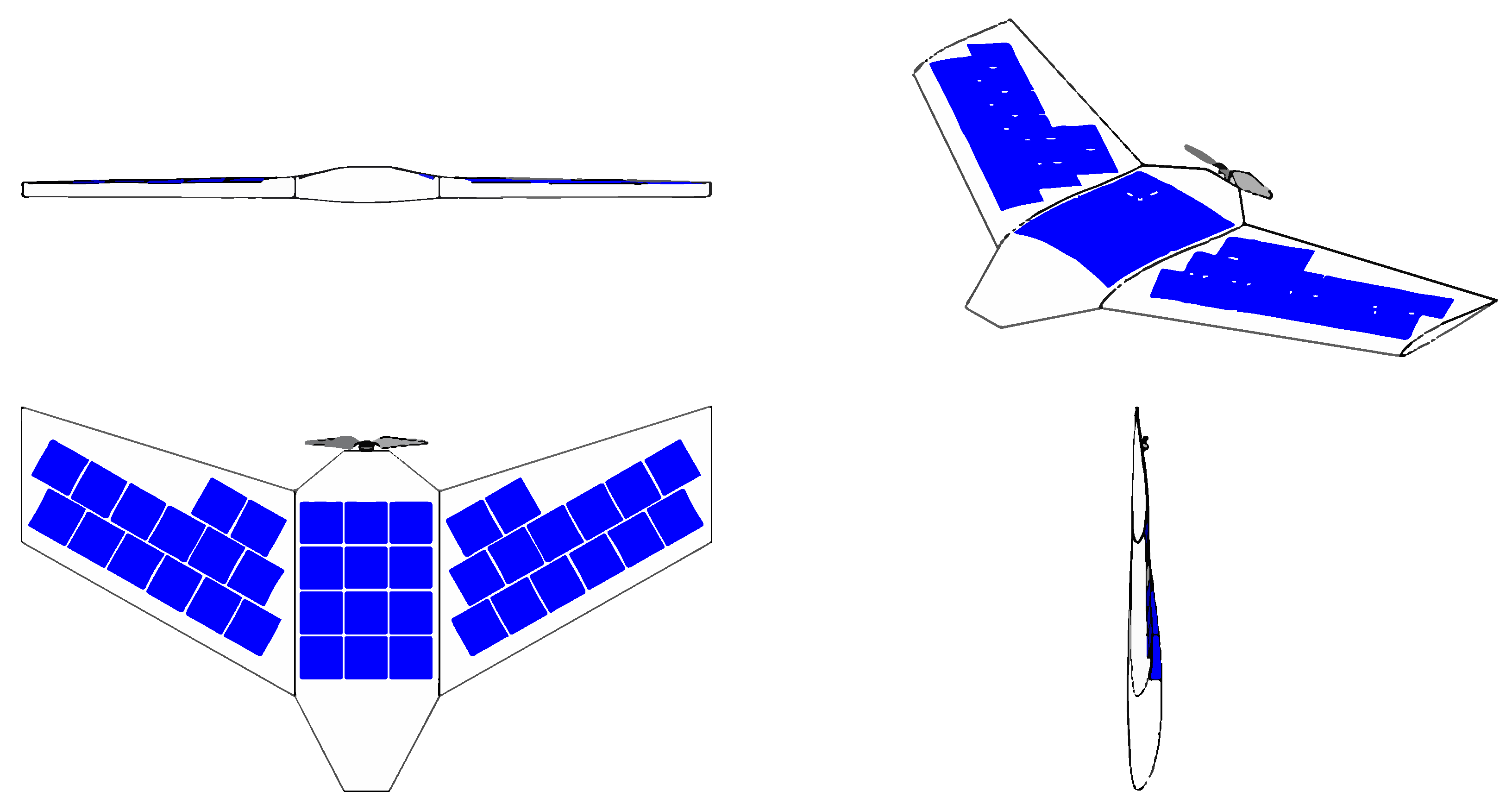
The SUAV investigated in this study adopts a low-aspect-ratio flying wing configuration, with its external shape illustrated in Figure 1. The wing features a moderate sweepback angle to ensure sufficient longitudinal stability and crosswind resistance. The fuselage is seamlessly blended with the wing, sharing the same airfoil profile. The propulsion system is mounted at the rear of the fuselage, utilizing a direct current(DC) brushless motor to directly drive the propeller.

The SUAV has a wingspan of 2 m and a fuselage length of 1 m, with key parameters summarized in

Table 1. Main parameter of the SUAV.

Parameter	Value	Unit
Wing Span	2020	mm
Mean Aerodynamic Chord	619	mm
Length	1000	mm
Wing Area	1.14	m2
Total Weight	3.0	kg
Battery Weight	0.9	kg
Cruise Speed	10	m/s
Cruise altitude	100	m

. It is designed to operate at a cruising altitude of 100 m and a cruising speed of 8 m/s. 40 Sunpower C60 solar cells (SunPower, San Jose, CA, USA) are installed on the upper surface of the wing.

The SUAV structure adopts a sandwich structure composed of PMI foam core and composite material panel. To prevent the solar cells from short-circuiting, the fiber material of the upper face sheet on the upper wing surface uses glass fiber, while the face sheets in other positions are made of carbon fiber composite materials. The propulsion system employs a 4006 brushless DC motor (SUNNYSKY, Guangzhou, China), matched with a 15 × 7 inch carbon fiber propeller, and is installed at the tail of the fuselage.

2.2. Aerodynamic Model of SUAV

During cruise flight, the UAV maintains a level and steady flight state, with balanced external forces in both the horizontal and vertical directions. Specifically, the lift force equals the gravitational force, and the thrust generated by the propulsion system equals the drag force encountered. The force balance equation can be written as

$$mg=L={\displaystyle \frac{1}{2}}\rho v^{2}S{C}_L$$

(1)

$$T=D={\displaystyle \frac{1}{2}}\rho v^{2}S{C}_D$$

(2)

The flight speed of the UAV can be derived from Equation (1).

$$v=\sqrt{{\displaystyle \frac{2mg}{C_L\rho S}}}$$

(3)

The flight power of the UAV can be calculated based on Equations (2) and (3).

$$P_{lev}=Dv={\displaystyle \frac{C_D}{C_L^{1.5}}}\sqrt{{\displaystyle \frac{2{\left(mg\right)}^3}{\rho S}}}$$

(4)

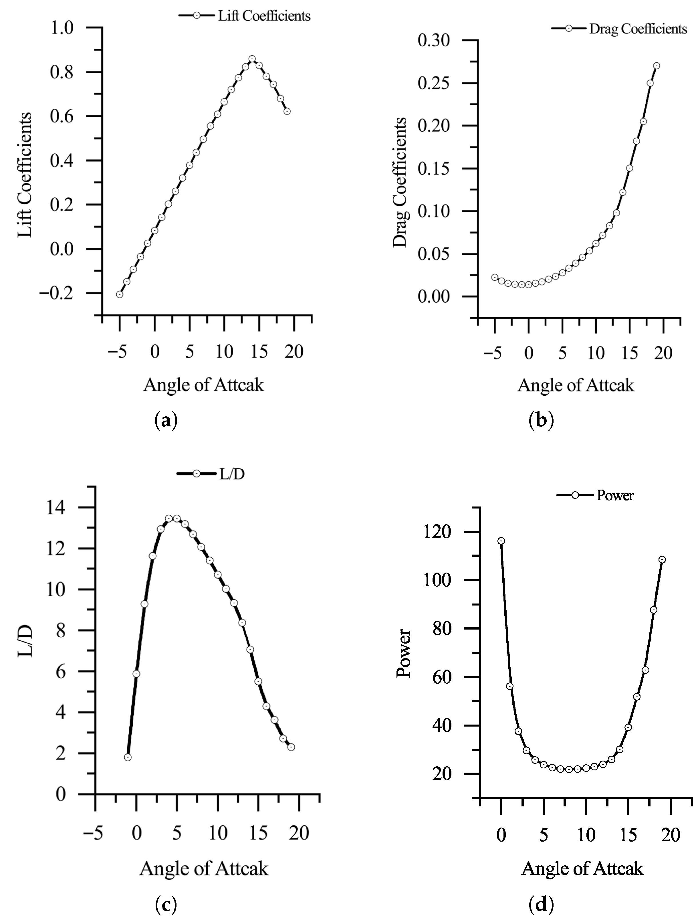
The $C_L$ and $C_D$ depend on parameters such as the configuration, airfoil shape, AoA, and Reynolds number of the SUAV. In this study CFD is employed to analyze the aerodynamics of the SUAV. The calculated lift and drag characteristics of a single SUAV are shown in Figure 2a–c, while the cruise power is presented in Figure 2d. At an AoA of 5°, the single SUAV achieves a maximum lift-to-drag ratio of 13.45. The maximum endurance state of the UAV corresponds to the minimum level flight power point. At an AoA of 8°, the minimum level flight power of the single SUAV is 23.4 W.

2.3. Energy Model of SUAV

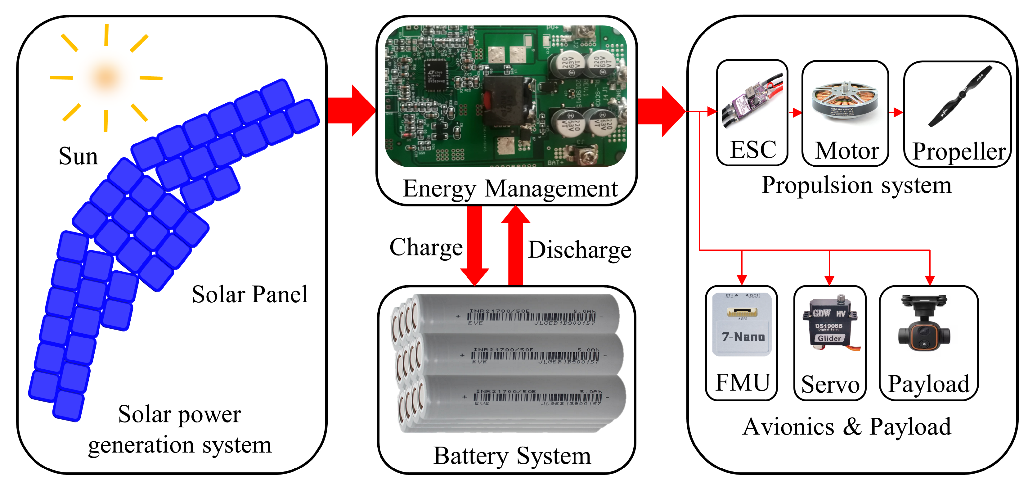
The architecture of the SUAV system is illustrated in Figure 3, which primarily consists of a solar power generation system, an energy storage battery system, an energy management system, an avionics & payload system and a propulsion system. The solar cell system converts solar radiation into electrical energy. During daytime operations, the energy storage system stores excess electricity generated by the solar cells and supplies power during nighttime to maintain the UAV’s operation. The energy management system regulates the power flow between the solar power generation system and the lithium battery energy storage system.The avionics system is responsible for stable flight control, mission execution, and communication functions. The propulsion system provides the necessary thrust for the UAV’s operation. Mission payloads are equipped according to specific operational requirements.

2.3.1. Solar Power Generation Model

Solar cells are one of the key systems of an SUAV. The power generation model of the solar cells is used to calculate the energy acquired by the UAV under different conditions. The power output of the solar cells is related to the received solar radiation energy, which is influenced by variables such as latitude, date, and time. To study the power generation capability of the solar cells, it is necessary to model the solar radiation. Duffie established an accurate solar radiation model [15], but its complexity stems from the emphasis on precision. Colozza et al. from NASA proposed a simplified method for estimating solar radiation during their research on high-altitude SUAVs [16]. Based on this model, this paper develops a solar radiation model suitable for the flight conditions of the UAV studied here.

The Earth’s orbit around the Sun is elliptical, resulting in variations in received solar radiation over the orbital period. The intensity of solar radiation energy at the top of the atmosphere on different dates throughout the year can be expressed by Equation (5):

$$I_0=I[1+0.033cos\left(2\pi {\displaystyle \frac{n}{365}}\right)]$$

(5)

where $I_0$ represents the solar radiation at the top of the atmosphere; I is the solar constant, typically taken as 1352 $\mathrm{W}/{\mathrm{m}}^2$; n denotes the day of the year, with n = 1 representing 1 January.

The Earth’s atmosphere further absorbs a portion of the solar radiation. The intensity of solar radiation reaching the ground can be expressed by Equation (6):

$$I_1=I_0\tau$$

(6)

where $\tau$ represents the solar attenuation factor. Since the SUAV studied in this paper operates at a low cruising altitude, is approximately taken as the standard sea-level value of 0.85 [17].

The SUAV investigated in this study is equipped with 40 Sunpower C60 solar cells, whose parameters are listed in

Table 2. Parameters of the solar cells.

Parameter	Symbol	Value
Area	$S_{\mathrm{Cell}}$	125 × 125 mm2
Number of Cells	N	40
Cell Conversion Efficiency	${\eta }_{\mathrm{Cell}}$	25%
Encapsulation Efficiency	${\eta }_{\mathrm{Encap}}$	95%

.

Considering 10% atmospheric scattering intensity and the incidence angle of sunlight relative to the solar cells, the electrical energy output of the solar cells can be expressed as

$$P_{\mathrm{cell}}=N{S}_{\mathrm{cell}}{\eta }_{\mathrm{cell}}{\eta }_{\mathrm{Encap}}\times (0.1\times I_1+I_{1}sin\theta )$$

(7)

where: $\theta$ represents the solar altitude angle, which can be expressed as

$$\theta =arcsin(sin\varphi sin\delta +cos\varphi cos\delta cos\omega )$$

(8)

where: $\phi$ represents the local latitude; $\delta$ and $\omega$ denote the solar declination angle and the hour angle, respectively, which can be expressed as

$$\left\{\begin{array}{c}\delta =23.45sin\left(2\pi {\displaystyle \frac{(n+284)}{360}}\right)\\ \omega =15(t-12)\end{array}\right.$$

(9)

where: n represents the day of the year; t denotes the time of day, with a value range of 0 to 24 and units in hours.

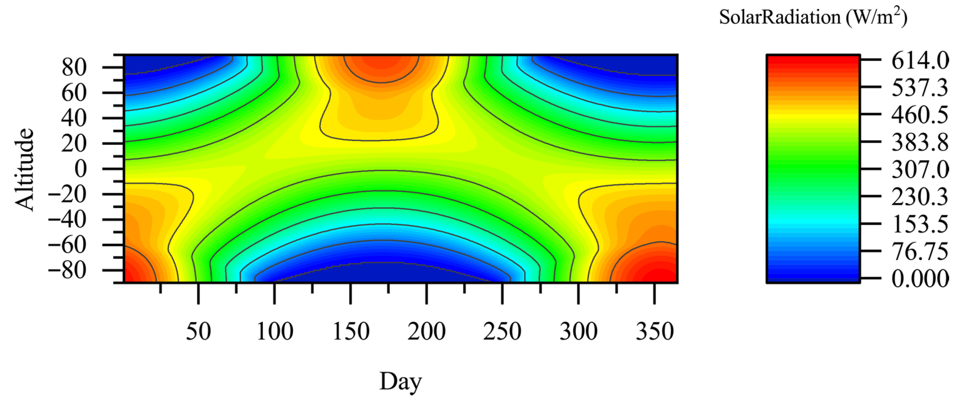
Using the above equations, the solar radiation at different times and latitudes is calculated. The resulted distribution of the average daily solar irradiance across various latitudes and dates is shown in Figure 4.

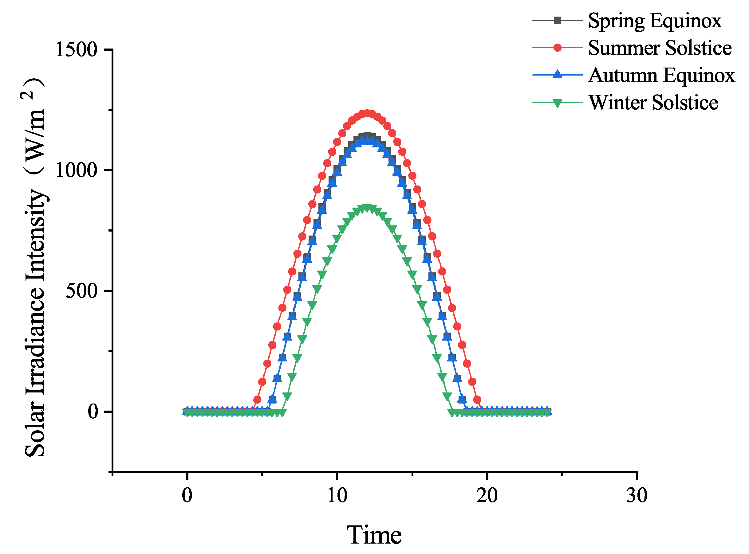
The output power of the SUAV studied in this paper across different dates of the year is shown in Figure 5.

SUAVs are characterized by their long endurance. Endurance performance analysis typically covers extended periods, and overly complex energy models can significantly increase computational difficulty. Therefore, the solar power generation model in this study incorporates several simplifications. Firstly, during cruise flight, the UAV undergoes only minor maneuvering angles. The model assumes uniform solar irradiation on the solar cells, neglecting the influence of the UAV’s flight attitude on the solar incidence angle. Furthermore, the UAV utilizes silicon-based solar cells, although their photoelectric conversion efficiency is affected by temperature [18], the temperature variation in solar cells during cruise flight is less than 20 °C, so the conversion efficiency is considered constant. In conclusion, as a tool for endurance performance trend analysis, the proposed model is reliable.

2.3.2. Battery Energy Storage Model

The energy storage system of the SUAV consists of 12 cylindrical lithium batteries with high energy density. The battery model utilized is the EVE 50E 26700 cylindrical cell (EVE, Huizhou, China), which has an energy density of 271 Wh/kg. To match the system voltage, the batteries are configured in a 6S3P arrangement (6 cells in series per group, with 3 groups in parallel), providing a total energy capacity of 342 wh. The performance parameters of a single battery cell are listed in

Table 3. Battery parameters.

Parameter	Symbol	Value
Nominal Capacity	$E_{\mathrm{Battery}}$	5000 mah
Rated Voltage	V	3.8 V
Discharge Efficiency	${\eta }_{\mathrm{Discharge}}$	96%
Charge Efficiency	${\eta }_{\mathrm{Charge}}$	96%

.

2.3.3. UAV Energy Management System

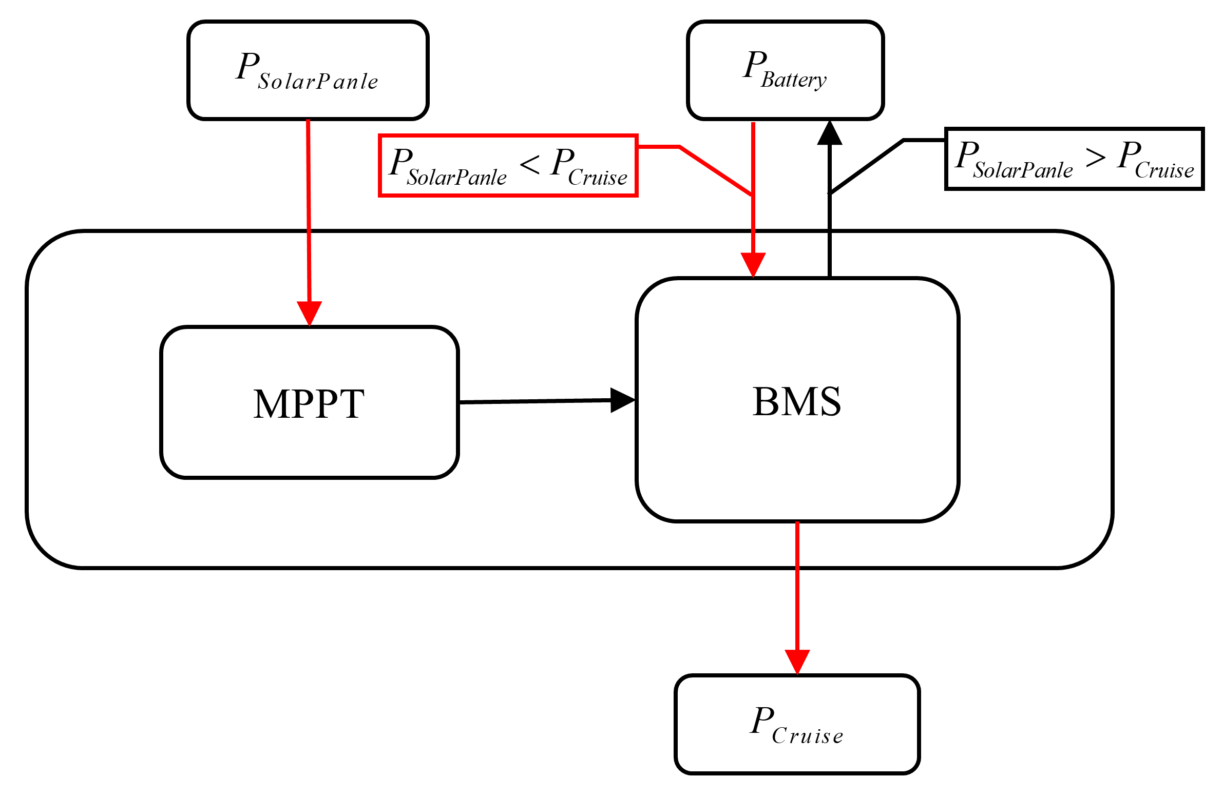
The workflow of the energy management system is illustrated in Figure 6. This system has two primary functions: Maximum Power Point Tracking (MPPT) to optimize the operational state of the solar cells and stabilize their output power near the maximum power point, achieving a conversion efficiency ${\eta }_{\mathrm{MPPT}}$ of 96% for this process; second, a Battery Management System (BMS) to manage the overall energy allocation of the UAV.

When the output power of the solar cells exceeds the total cruise power requirement of the UAV, a portion of the electricity is used to power the various systems of the UAV, while the remaining portion charges the lithium batteries. When the output power of the solar cells is insufficient to meet the total cruise power demand, both the solar cells and the lithium batteries discharge simultaneously to support the operation of the UAV’s systems.

2.3.4. UAV Energy Consumption Model

During level and steady flight, the energy consumption of the UAV can be expressed as

$$P_{\mathrm{tot}}=P_{\mathrm{pay}}+P_{\mathrm{req}}+P_{\mathrm{avr}}$$

(10)

where: $P_{\mathrm{tot}}$ denotes the power consumed by the mission payload carried by the SUAV, which is a constant value. In this study, the payload power is 2 W; $P_{\mathrm{avr}}$ represents the power consumed by the onboard electronic system, also a constant value. For the SUAV investigated here, the avionics power is 2 W; $P_{\mathrm{req}}$ indicates the power required for level and steady flight of the SUAV, which can be expressed as

$$P_{\mathrm{req}}={\displaystyle \frac{P_{\mathrm{lev}}}{{\eta }_{\mathrm{prop}}{\eta }_{\mathrm{mot}}{\eta }_{\mathrm{ESC}}}}$$

(11)

where: $P_{\mathrm{lev}}$ denotes the minimum power required for level and steady flight of the UAV, as derived from the aerodynamic model of the SUAV; ${\eta }_{\mathrm{prop}}$ represents the conversion efficiency of the propeller; ${\eta }_{\mathrm{motor}}$ indicates the conversion efficiency of the electric motor; ${\eta }_{\mathrm{ESC}}$ symbolizes the conversion efficiency of the brushless electronic speed controller (ESC).

3. Aerodynamic Modeling and Optimization of Solar-Powered UAV Formations

In this section, the aerodynamic model for the SUAV formation is established, and the formation parameters are optimized to minimize cruise power. First, the concept of SUAV formations and their key parameters are introduced. CFD is then employed to analyze the aerodynamic performance of the formation. Subsequently, a surrogate model is constructed to represent the relationship between the flight parameters and aerodynamic characteristics of the SUAV formation. Finally, with the objective of minimizing the cruise power of the formation, the parameters are optimized based on the surrogate model.

3.1. Concept and Design Variables of Solar-Powered UAV Formations

Chen et al. investigated the optimization of aerodynamic performance for different formation configurations [19]. They used CFD to analyze the aerodynamics of both “linear” and “V-shaped” formations. The results indicated that the V-shaped formation provides greater aerodynamic benefits for the trailing UAVs.

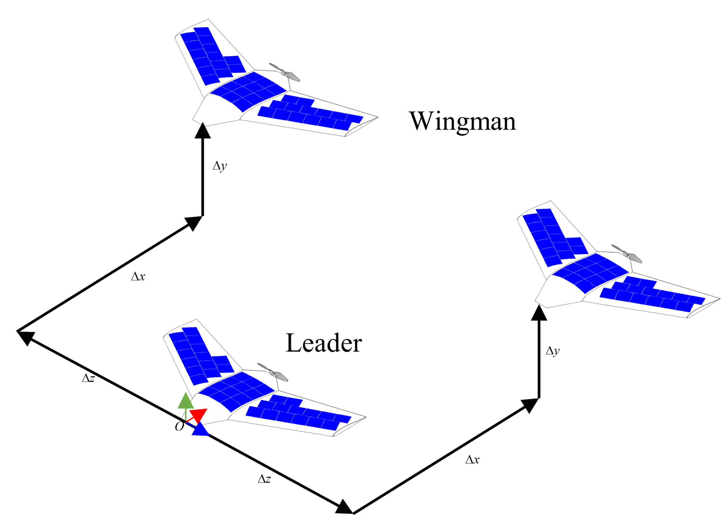
The SUAV formation studied in this paper is illustrated in Figure 7. It adopts a symmetric V-shaped formation, with one leader UAV flying at the front and two accompanying UAVs positioned symmetrically behind on the left and right sides. $\Delta$x denotes the longitudinal separation between the leader and the wingmans UAVs along the flight direction; $\Delta$z represents the vertical separation between the leader and the wingmans; $\Delta$y indicates the lateral separation along the wingspan direction. The nose of the leader UAV is defined as the origin of the coordinate system, with the two wingmans symmetrically distributed relative to the $xoy$ plane.

To investigate the formation parameters that yield optimal aerodynamic benefits, it is essential first to identify the parameters influencing these gains. The aerodynamic advantages of formation flight are affected by variables such as the relative positions of the leader and follower UAVs, as well as the AoA. Zhang et al. conducted aerodynamics modeling and analysis of close formation flight [20]. Based on elliptical lift distribution and lifting-line theory, they proposed and validated a model for calculating formation aerodynamics. The study concluded that, for aircraft in level and steady formation flight, the optimal formation parameters occur at a lateral separation equal to 0.95 times the wingspan and a vertical separation of zero. Furthermore, this optimal position varies with the AoA. It is generally accepted that when the longitudinal separation exceeds three times the wingspan, the formation is considered “loose flight,” where aerodynamic coupling between UAVs is weak or even negligible [21]. Finally, the design variables and their upper/lower bounds selected for the SUAV formation in this study are listed in

Table 4. Design variables of the SUAV formation.

Parameter	Symbol	Value	Unit
x-direction distance	$\Delta$x	2–4	m
y-direction distance	$\Delta$y	−0.2–0.2	m
z-direction distance	$\Delta$z	1–3	m
Leader AoA	${\alpha }_{\mathrm{Leader}}$	2–10	deg
Wingman AoA	${\alpha }_{\mathrm{Wingman}}$	2–10	deg

.

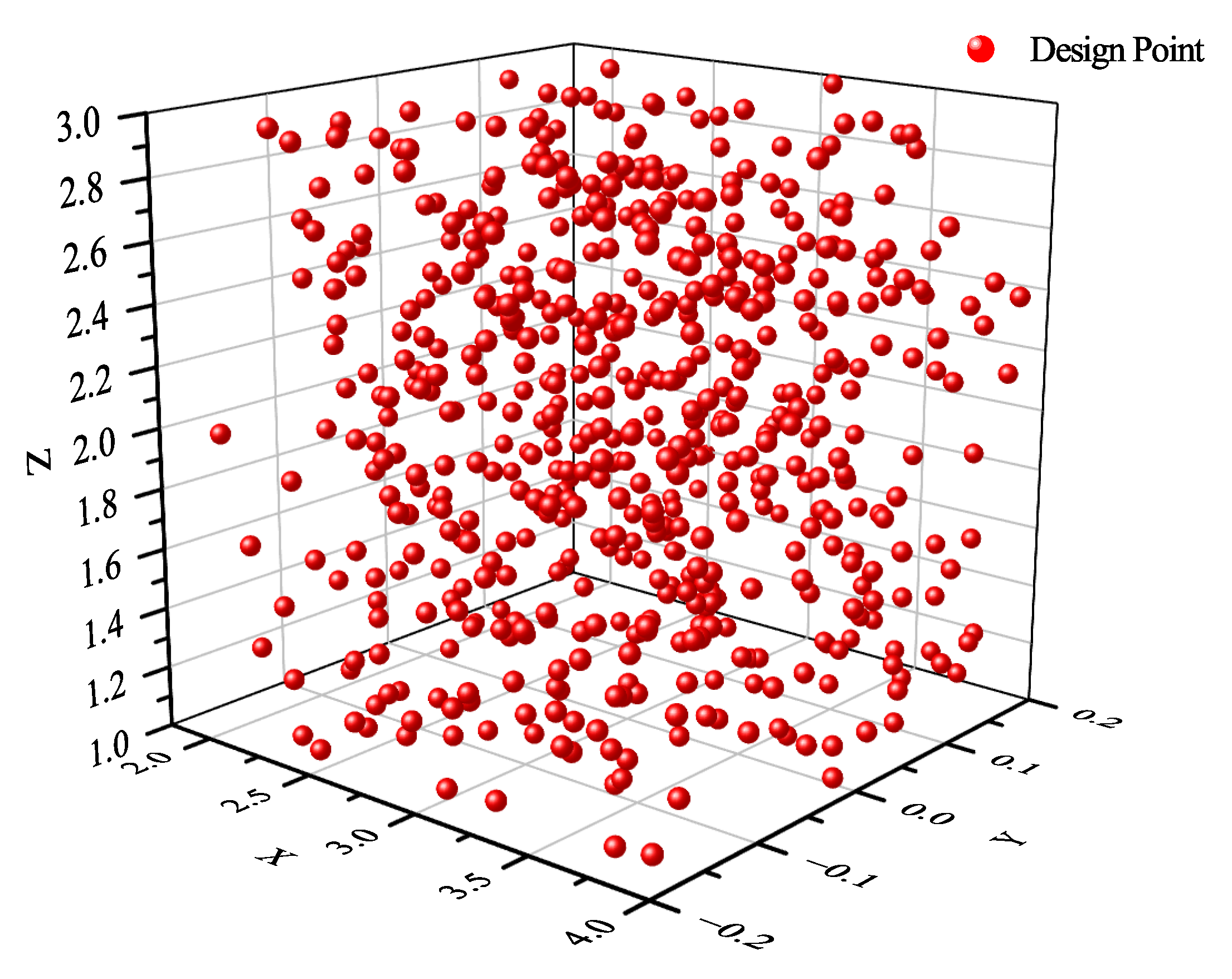
To construct a surrogate model approximating the relationship between the formation parameters and aerodynamic performance of SUAVs, it is necessary to select multiple distinct design points within the design domain. The minimum number of required design points is positively correlated with the dimensionality of the design variables. Generally, the accuracy of the surrogate model improves as the number of design points increases.Common experimental design methods include Full Factorial Design, Fractional Factorial Design, Orthogonal Arrays, and Latin Hypercube Design. Comparing the Latin Hypercube Design with other methods reveals its superior uniformity in design space coverage and its suitability for the high-dimensional problem in this study [22]. To ensure high model accuracy, this study employs Latin Hypercube Design to select 600 design points within the design domain for further computation.The distribution of the design points within the design space is shown in Figure 8.

3.2. Aerodynamic Calculation of Formation Flight

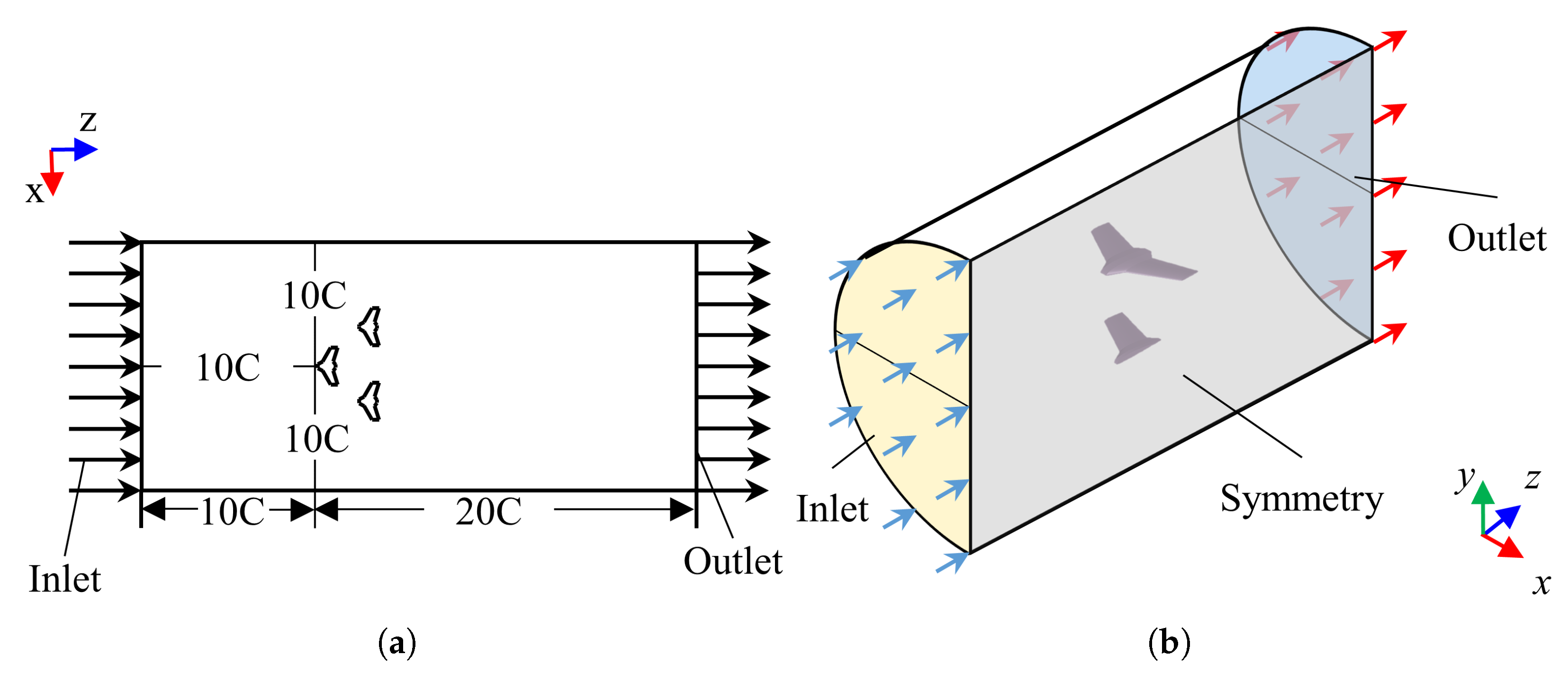
The model was constructed using Ansys Geometry, with the design variables listed in Table 4 defined as variable parameters. Subsequent automated solutions can be performed by enabling the software to automatically read the variable values of each design point. The fluid domain model for the SUAV formation is shown in Figure 9a. The coordinate system is consistent with the leader-nose coordinate system described in Section 3.1. The computational domain is a cylindrical region with a radius of 20 m (ten times the wingspan of the UAV) and a length of 60 m. The inlet boundary condition of the fluid domain is set as a velocity inlet, while the outlet is defined as a pressure outlet. The model and flow solution exhibit physical symmetry about the XZ-plane, giving a computational advantage that allows half of the fluid domain to be used by applying a symmetry boundary condition. This reduces the number of grid cells and the associated computational expense. The fluid domain model and boundary conditions used for the CFD calculations are illustrated in Figure 9b.

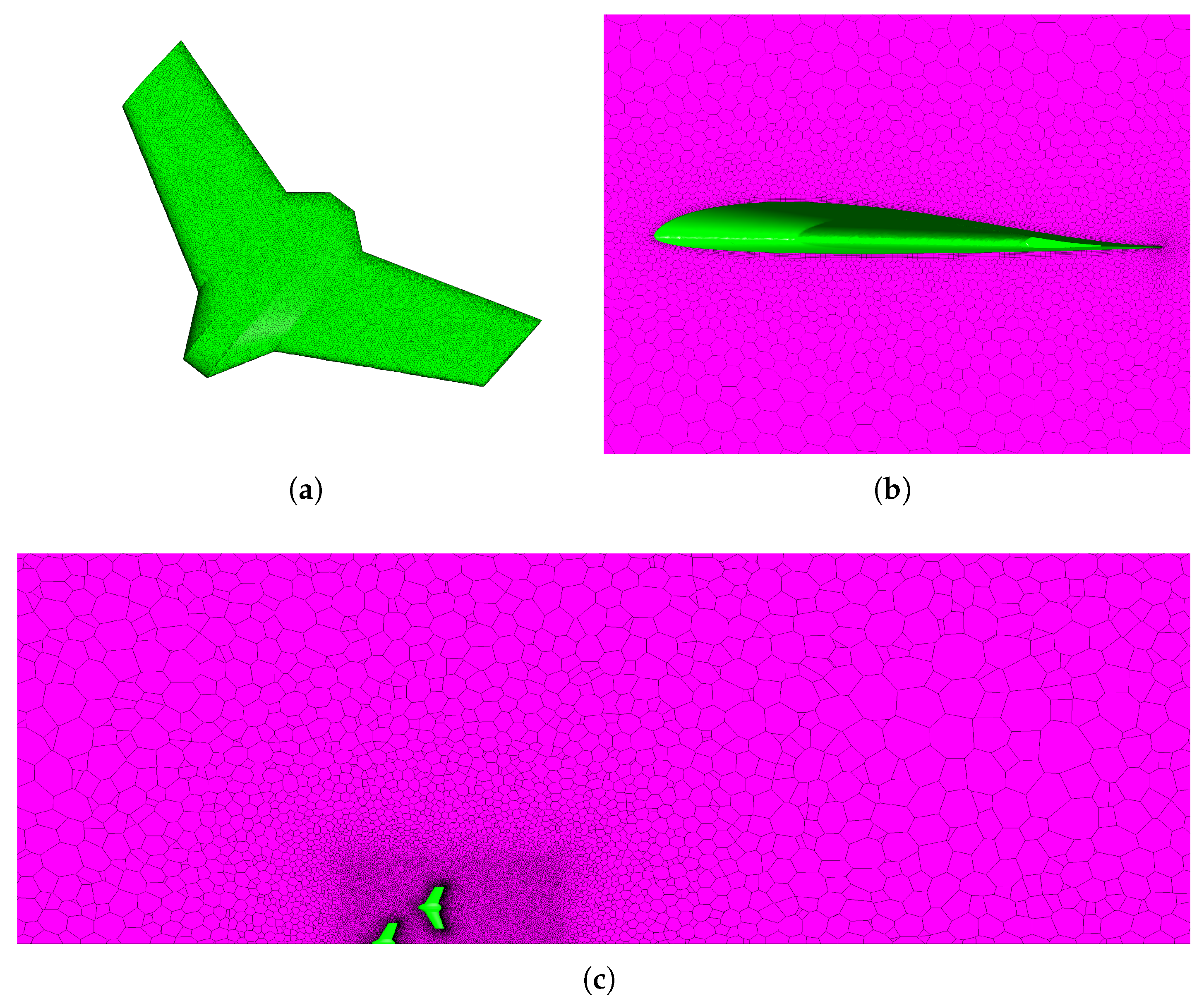
The mesh was generated using Ansys Mesh software. All mesh elements are unstructured tetrahedral cells, with a surface mesh size of 0.005 m applied to the UAV surfaces. The resulting surface mesh of the UAV is shown in Figure 10a. To improve computational accuracy, a five-layer boundary layer mesh was generated on the surface of the SUAV. The boundary layer mesh is illustrated in Figure 10b. The initial mesh consists of 3.16 million cells. The mesh of the fluid domain is presented in Figure 10c.

This study employs Ansys Fluent software for solution computation. The Navier–Stokes equations are discretized using the finite volume method, and a pressure-based solver is adopted. The k-$\omega$ SST turbulence model is selected for turbulence modeling [23]. The cruise state of the SUAV investigated in this study involves low-altitude and low-speed flight; thus, the initial conditions for the flow field are set as follows:

1.

The flight altitude is low-altitude, and sea-level atmospheric parameters are directly used for calculation. The corresponding atmospheric density is 1.225 $\mathrm{kg}/{\mathrm{m}}^3$, atmospheric pressure is 101,325 Pa, temperature is 288.5 K, and viscosity is $1.78\times {10}^{-5}$$\mathrm{kg}/\mathrm{ms}$.

2.

The flow field inlet velocity is set to 8 $\mathrm{m}/\mathrm{s}$.

3.

The convergence criterion is set such that the globally scaled residuals of the continuity and momentum equations decrease to 0.0001.

The 600 design points are divided into 5 groups and distributed across five computers for simultaneous solving. All computers are configured with an Intel Core i7-9700F (Intel, Santa Clara, CA, USA) (8 Cores, 3 GHz base frequency). The computation time required is 48 h.

3.3. Solar-Powered UAV Formation Aerodynamic Model

Approximate modeling is a method that utilizes empirical formulas to establish quantitative relationships between input and output data. Due to its fast convergence and high stability, the Orthogonal Polynomial Model has been widely adopted. After considering computational cost and accuracy requirements, this study selects the Orthogonal Polynomial Model to develop the aerodynamic model for SUAV formations.

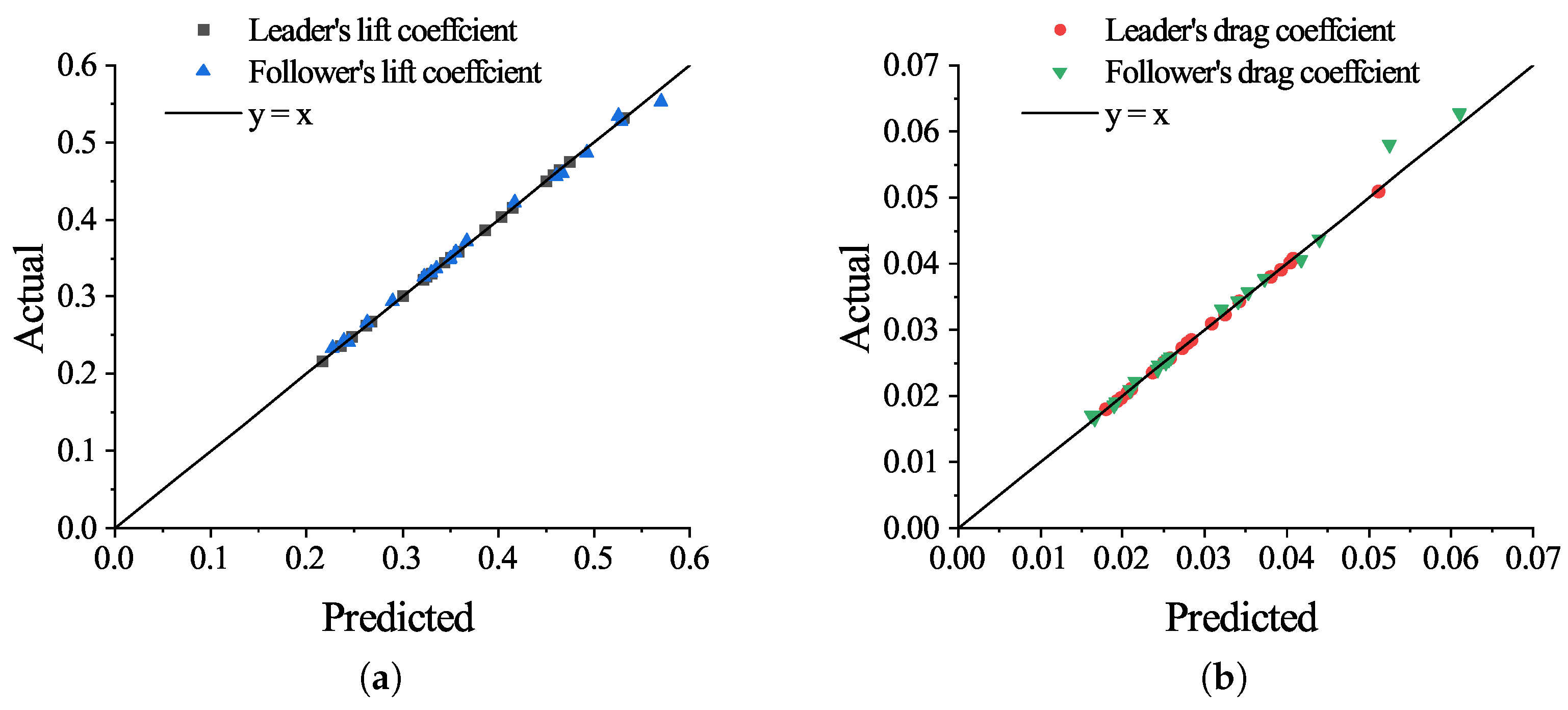
From 600 design points, 20 sets of data were randomly selected to validate the accuracy of the approximate model. Diagonal error plots and line error plots for each parameter are shown in Figure 11.

The diagonal error plot indicates strong alignment between the actual and predicted values, as both are distributed near the 45° line. Similarly, the line error plot shows the predicted curve tracking the actual values with high fidelity, resulting in significant overlap. These observations indicate minimal error and validate the effective performance of the approximate model.

3.4. Solar-Powered UAV Formation Parameter Optimization

The parameter optimization process for SUAV formations based on a surrogate model begins by defining the design variables, objective function, and constraints for the design.

1.

Design variables: Design variables are a set of parameters that can be controlled and modified during the optimization process. The variables and their corresponding upper and lower bounds used in the parameter optimization of the SUAV formation are listed in Table 4. These can be expressed in the form of Equation (12):

$$X=[\Delta x,\Delta y,\Delta z,{\alpha }_{\mathrm{Leader}},{\alpha }_{\mathrm{Wingman}}]$$

(12)

2.

Objective function: The objective of the optimization is to minimize the power consumption during formation flight. The cruise power of a single SUAV is given by Equation (4). The cruise power of the SUAV formation can be expressed as

$$P_{lev-Formation}=\left({\displaystyle \frac{C_{\mathrm{D}-\mathrm{Leader}}}{C_{\mathrm{L}-\mathrm{Leader}}^{1.5}}}+2{\displaystyle \frac{C_{\mathrm{D}-\mathrm{Wingman}}}{C_{\mathrm{L}-\mathrm{Wingman}}^{1.5}}}\right)\sqrt{{\displaystyle \frac{2{\left(mg\right)}^3}{\rho S}}}$$

(13)

During the optimization process, the objective function can be regarded as a function of the design variables. The optimization objective can be expressed as

$$f\left(X\right)=P_{\mathrm{lev}-\mathrm{Formation}}=f(\Delta x,\Delta y,\Delta z,{\alpha }_{\mathrm{Leader}},{\alpha }_{\mathrm{Wingman}})$$

(14)

3.

Constraints: Constraints refer to the conditions that must be satisfied by the design points during the optimization process. In the context of level cruise flight of an SUAV formation, the leader and wingman are required to maintain the same airspeed. Additionally, since both aircraft have identical takeoff weights, their lift coefficients must also be equal. The constraints in the optimization process can be expressed as

$${\mathrm{C}}_{\mathrm{L}-\mathrm{Leader}}=C_{\mathrm{L}-\mathrm{Wingman}}$$

(15)

4.

Optimization design: The mathematical objective of the optimization design is to identify a set of design variables within the design space that satisfy all constraints while minimizing the value of the objective function. The optimization design for the SUAV formation can be expressed as

$$\left\{\begin{array}{c}find:X=[X,Y,Z,{\alpha }_{\mathrm{Leader}},{\alpha }_{\mathrm{Wingman}}]\hfill \\ minimize:f\left(x\right)=P_{\mathrm{lev}-\mathrm{Formation}}=f(X,Y,Z,{\alpha }_{\mathrm{Leader}},{\alpha }_{\mathrm{Wingman}})\hfill \\ subjectto:{\mathrm{C}}_{\mathrm{L}-\mathrm{Leader}}=C_{\mathrm{L}-\mathrm{Wingman}}\hfill \end{array}\right.$$

(16)

The optimization calculations for the model were conducted using the sequential quadratic programming algorithm (SQP) and the multi-island genetic algorithm (MIGA), respectively. The SQP algorithm is suitable for local fine optimization with high efficiency, while the MIGA algorithm is effective for global search; comparing the two ensures both computational efficiency and the acquisition of a globally optimal solution. The SQP method terminated after 89 iterations, while the MIGA method completed 1000 generations. The optimization results are presented in

Table 5. Formation parameter optimization calculation results.

Parameter	SQP	MIGA	Unit
$\mathrm{Iteration}\mathrm{Count}$	89	1001	-
$\mathrm{Time}\mathrm{Cost}$	40	445	s
$\Delta x$	2.00	2.44	m
$\Delta y$	0.00	−0.03	m
$\Delta z$	1.75	1.62	m
${\alpha }_{Leader}$	7.2	7.0	deg
${\alpha }_{Wingman}$	6.1	6.2	deg
$C_{{\mathrm{L}}_{\mathrm{Leader}}}$	0.442	0.425	-
$C_{{\mathrm{D}}_{\mathrm{Leader}}}$	0.036	0.035	-
$C_{{\mathrm{L}}_{\mathrm{Wingman}}}$	0.442	0.434	-
$C_{{\mathrm{D}}_{\mathrm{Wingman}}}$	0.028	0.027	-
$C_{{\mathrm{P}}_{\mathrm{Formation}}}$	61.10	62.1	W

. It can be observed that for the optimization of this model, the SQP method demonstrates higher computational efficiency and solution accuracy.

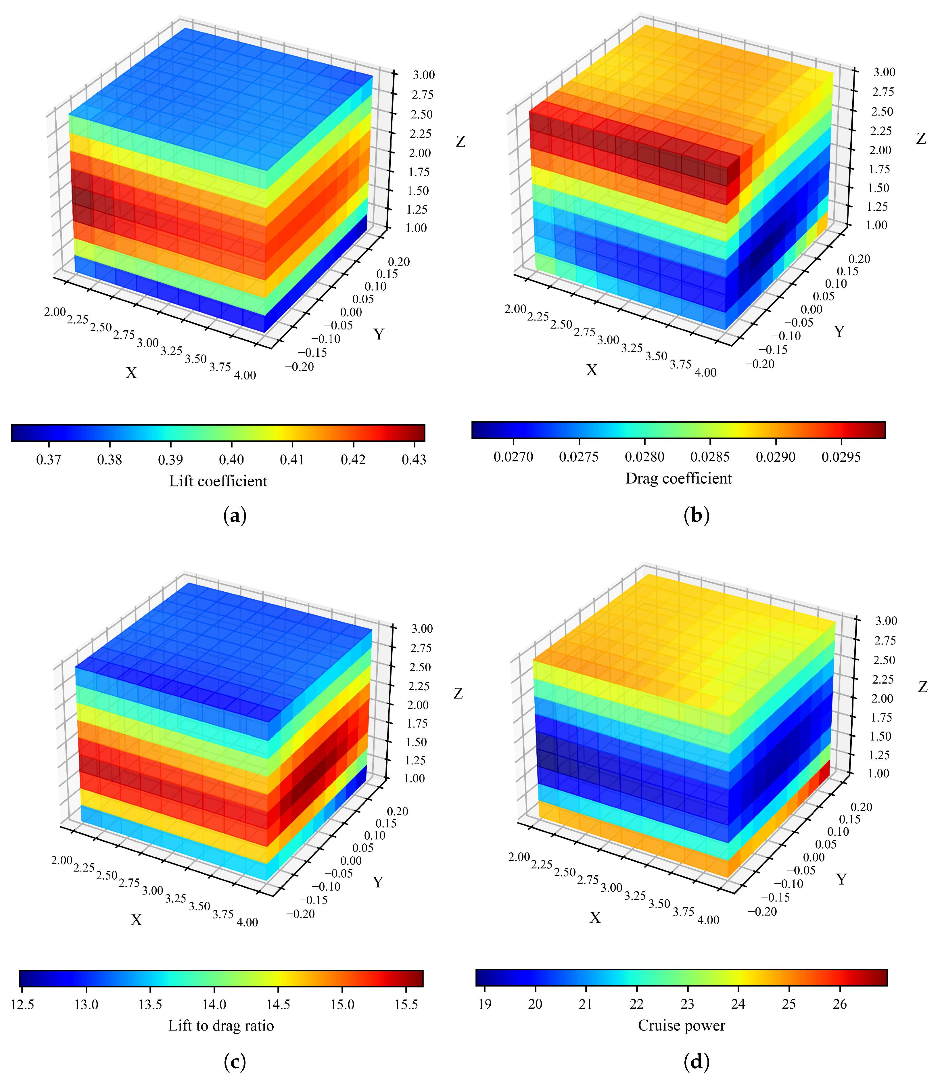
The aerodynamic performance of the wingman at a lead aircraft AoA of 7.2° and a wingman AoA of 6.1° was visually output, and the results are shown in Figure 12. The influence of formation position parameters on the wingman’s aerodynamic performance can be easily observed. The vertical distance between the lead aircraft and the wingman has a relatively minor impact on the aerodynamic gain effect. The maximum lift-to-drag ratio occurs at a lateral distance of 1.75 m between the lead aircraft and the wingman, which is approximately 0.875 times the wingspan length. This value is slightly higher than the $\pi /4$ times wingspan predicted by the formula.

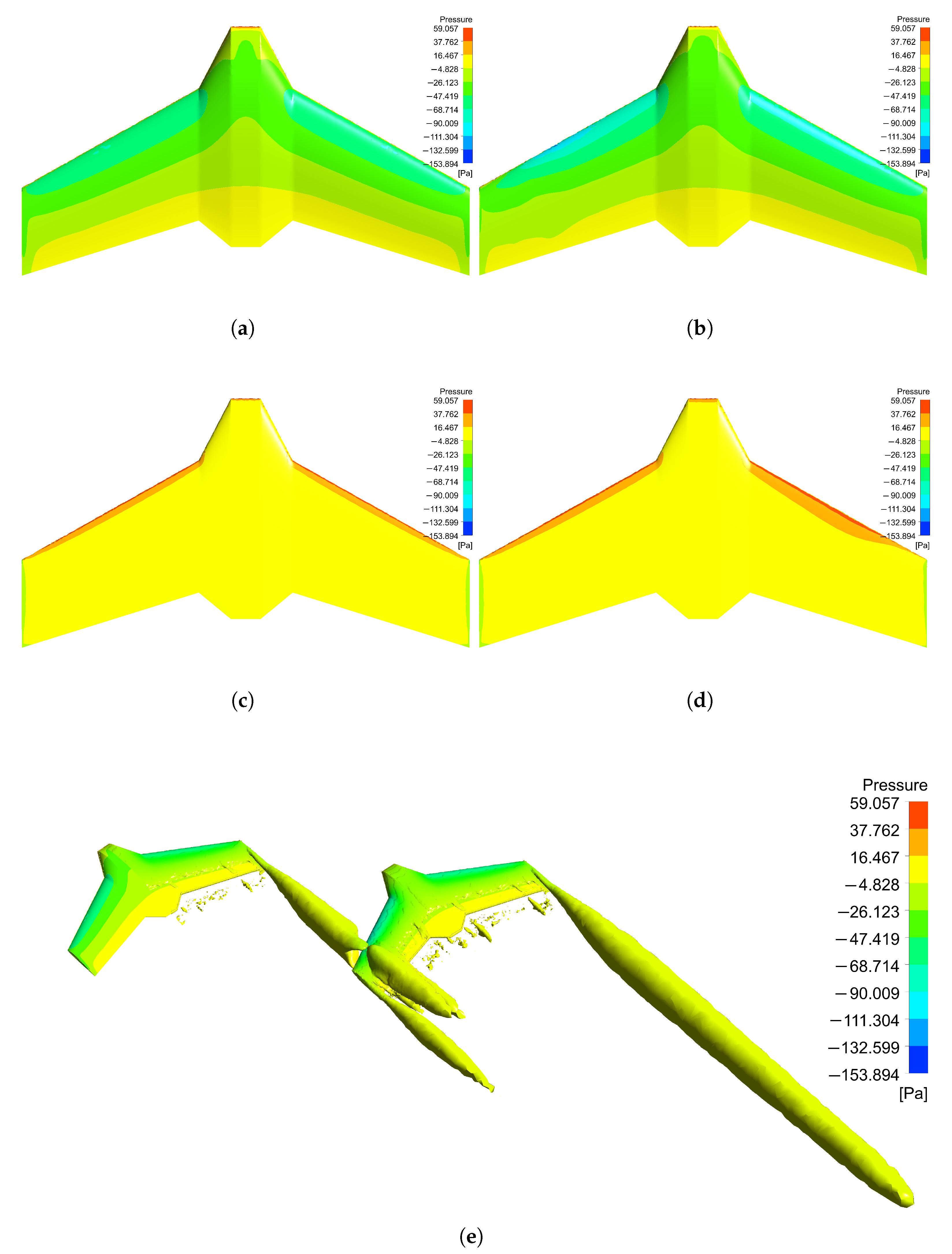
To validate the accuracy of the optimization results, CFD simulations were performed using the optimized formation parameters. The flow field structure of the optimized SUAV formation was analyzed. The results are presented in Figure 13. The pressure distributions on the surfaces of the leader and wingman UAVs are shown in Figure 13a–d. It can be observed that the pressure on the upper surface of the wingman’s left wing is significantly lower than that on the right wing, and the area of the high-pressure zone on the lower surface is larger than that on the right wing. This is because the left wing is within the influence area of the wingtip vortex generated by the lead aircraft, resulting in an increase in the wingman’s lift. Additionally, the reduced pressure at the leading edge of the left wing of the wingman reduces the pressure drag acting on the wing, leading to a decrease in the wingman’s overall drag.

The Q-criterion was employed to identify vortex structures in the flow field. The Q-value in the flow field is defined by the following equation:

$$Q={\displaystyle \frac{1}{2}}\left({∥\Omega ∥}^2-{∥S∥}^2\right)$$

(17)

In the equation, $\Omega$ represents the rotation tensor of the flow field, and S denotes the strain rate tensor. When Q > 0, rotational motion dominates, indicating the possible presence of a vortex structure in the region. The isosurface of Q = 0.002 in the flow field of the SUAV formation is shown in Figure 13e. It can be seen that the wingtip vortex of the wingman’s left wing is strongly disturbed by that of the leader’s right wing. Consequently, the downwash caused by the wingman’s wingtip vortex is strongly suppressed by the upwash generated by the leader. As a classic aerodynamic view, most of the induced drag of an aircraft in subsonic flight stems from the downwash of wingtip vortices. Therefore, due to the reduction in downwash, the drag coefficient of the wingman decreases.

4. Analysis of Endurance Performance for Solar-Powered UAV Formations

Aerodynamic calculations for the SUAV formation demonstrate that formation flight effectively increases the lift-to-drag ratio of the UAV group and reduces the cruise power requirement. This section presents energy-based simulations to evaluate the endurance time of both a single SUAV and the formation in flight. The impact of formation flight on endurance time range of SUAVs is investigated.

4.1. Energy Balance Simulation

Since solar radiation is symmetric around the summer solstice, the simulation of the theoretical endurance time of the UAV starts at 12:00 noon on the summer solstice. The following assumptions are made regarding the state of the UAV during simulation:

1.

Due to the symmetric nature of the simulation process, the initial State of Charge (SOC) of the energy storage battery is set to 50%.

2.

In the simulation, cruise power is treated as constant. This is because the durations of takeoff, climb, and landing phases are extremely short compared to the cruise phase.

3.

During flight, the SUAV formation may need to adjust its configuration based on the remaining battery levels of individual UAVs. Because of the significantly shorter duration of the formation adjustment compared to the cruise phase, its effect on cruise power is disregarded in the simulation.

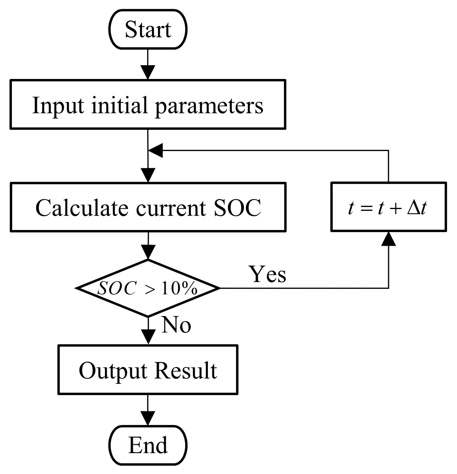
An energy simulation program for SUAVs is developed in the Python 3.9 environment, and the schematic diagram of the program structure is presented in Figure 14. In each iteration, the input power of the solar panel system and the power consumption of the UAV are calculated based on the current time step. The SOC information is then updated according to the net energy change. The simulation terminates once the SOC falls below 10%, at which point the energy simulation results are output.

The cruise power for a single SUAV is provided in Section 2.2 and Section 2.3. The level-flight power for the SUAV formation is derived from the optimization calculations in Section 3.4. Substituting into Equations (10) and (16), the cruise power of the SUAV formation can be expressed as

$$P_{\mathrm{Formation}}=3\times (P_{\mathrm{pay}}+P_{\mathrm{avr}})+{\displaystyle \frac{P_{\mathrm{lev}-\mathrm{Formation}}}{{\eta }_{\mathrm{prop}}{\eta }_{\mathrm{mot}}{\eta }_{\mathrm{ESC}}}}$$

(18)

The initial parameters for the energy simulation of both the single SUAV and the formation are listed in

Table 6. Initial conditions for energy simulation.

Parameter	Symbol	Single SUAV	SUAV Formation
Cruising power	$P_{\mathrm{Cruise}}$	35.1 w	95.8 w
Battery capacity	$E_{\mathrm{battery}}$	342 wh	1026 wh
Number of solar cells	$N_{\mathrm{Cell}}$	40	120

. The simulation latitudes are set to 45° N, 50° N, and 60° N.

4.2. Endurance Performance

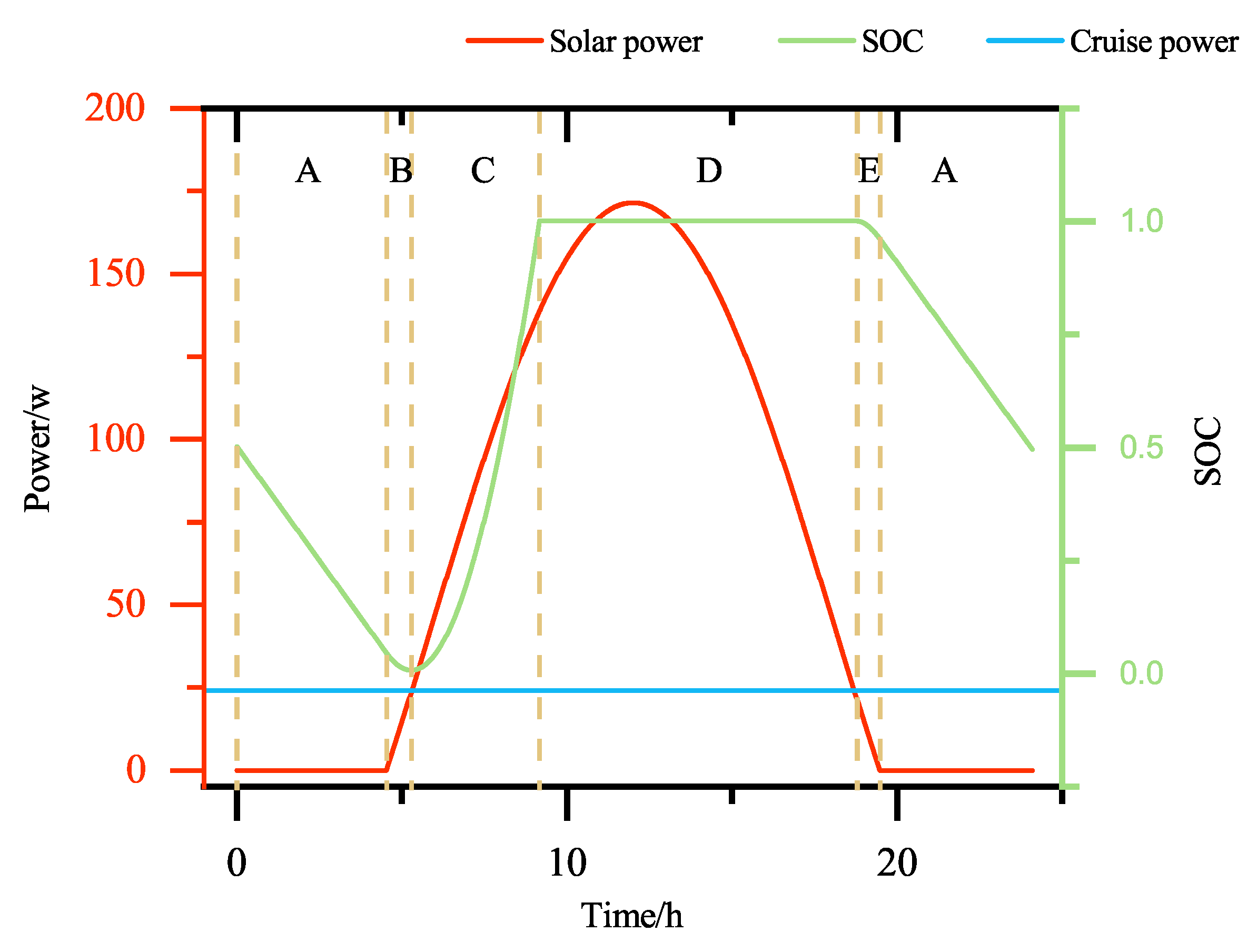
The simulation of daily flight energy for the SUAV is shown in Figure 15. Based on the power generation capacity of the solar cell system and the cruising power consumption of the UAV, the process can be divided into five stages. In Stage A, the output power of the solar cell system is zero, and the electrical energy consumed by the UAV system is supplied by the battery. In Stage B, both the solar cell system and the battery provide electrical power. In Stage C, part of the electricity generated by the solar cells is used to sustain the UAV’s consumption, while the excess portion charges the battery. In Stage D, the battery is fully charged, and the electricity generated by the solar cells is used for the UAV’s consumption. Any surplus energy can be utilized for climbing or other mission-specific actions. Stage E is similar to Stage B, with both the solar cells and the energy storage battery supplying power. After this, the cycle returns to Stages A through E. It can be observed that the lowest battery state of charge (${\mathrm{SOC}}_{\min }$) occurs at the critical point between Stage B and Stage C. At this point, the output power of the solar cells equals the power consumption of the UAV. During the energy simulation process, the value of the ${\mathrm{SOC}}_{\min }$ can be used to determine whether the UAV can continue maintaining its cruising state.

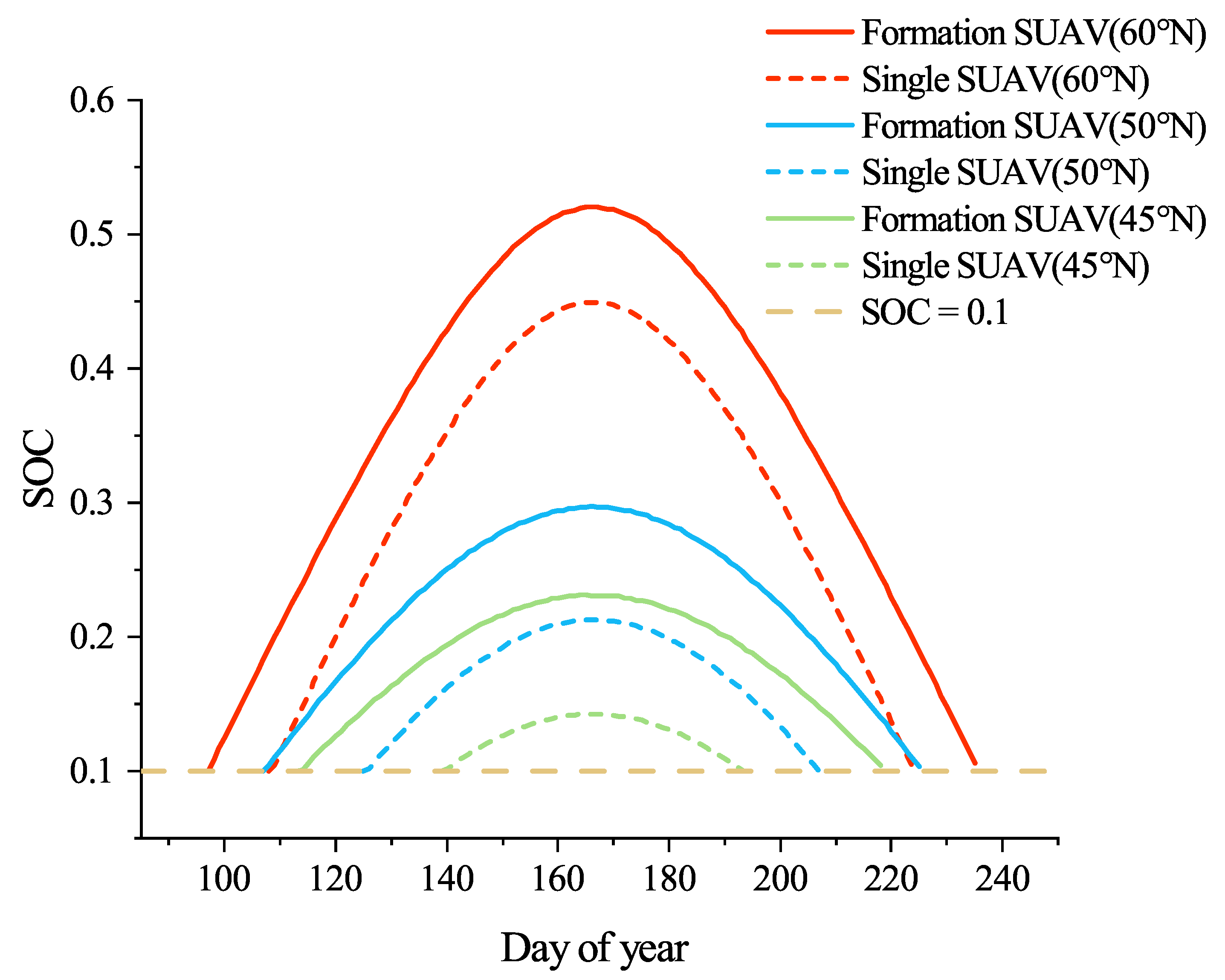
The data from Table 6 is used as the initial parameters for energy simulation of both the single UAV and the UAV formation. To balance computational efficiency and accuracy, the simulation time step $\Delta t$ is set to 0.5 min. To ensure sufficient safety margin for the SUAV, the simulation is terminated when ${\mathrm{SOC}}_{\min }$ below 0.1. The ${\mathrm{SOC}}_{\min }$ values during the energy simulation of the SUAV are shown in Figure 16. The results indicate that at a latitude of 45° N, the endurance of a single SUAV is 55 days, while that of the UAV formation is 106 days. At 50° N, the endurance of a single SUAV is 83 days, compared to 119 days for the UAV formation. At 60° N, the endurance of a single SUAV is 117 days, whereas the UAV formation achieves 139 days.

5. Results

This study evaluates the impact of formation flight on the lift-to-drag characteristics and endurance performance of SUAVs. A surrogate model was established to represent the relationship between formation parameters and aerodynamic performance. The surrogate model was employed to optimize the formation parameters, resulting in a set of values that minimize the cruise power of the SUAV formation. An energy model for SUAVs was also developed. Energy balance simulations were conducted for both a single UAV and a formation of SUAVs, providing theoretical endurance dates under different conditions. Based on the numerical results obtained, the main conclusions of this study are as follows:

1.

Formation flight can effectively improve the lift-to-drag ratio of UAVs and reduce their cruising power. Compared to a single SUAV, the maximum lift-to-drag ratio of the wingman in the formation increased by 15%.

2.

The minimum cruising power of a three-aircraft V-formation SUAV is 2.5 times that of a single SUAV. Compared to the single SUAV, the cruising power of the lead aircraft in the formation increased by 3.4%, while the flight power of the wingman decreased by 21%.

3.

The results show that under the conditions of 45° N, 50° N, and 60°N latitudes, the SUAV formation configuration increased endurance time by 92.7%, 43.3%, and 18.8%, respectively, compared to the single-UAV configuration. The endurance benefit gained from formation flight decreases with increasing latitude.

This study investigates the influence of formation flight on aerodynamic and endurance parameters of SUAVs. The discussion focused specifically on a three-UAV V-shaped formation, and the results demonstrate that formation flight can significantly enhance the endurance performance of SUAVs. If the scale of the formation is further increased, it may be possible to achieve year-round continuous flight for small SUAVs through formation flight. This study did not consider the impact of formation attitude disturbance and obstacle avoidance; future research can integrate autonomous navigation technology to explore dynamic formation optimization and achieve year-round continuous flight of small SUAVs.

References

1. Mohsan, S.A.H.; Khan, M.A.; Noor, F.; Ullah, I.; Alsharif, M.H. Towards the unmanned aerial vehicles (UAVs): A comprehensive review. Drones 2022, 6, 147. [Google Scholar] [CrossRef]
2. Boucher, R. History of solar flight. In Proceedings of the 20th Joint Propulsion Conference, Cincinnati, OH, USA, 11–13 June 1984; p. 1429. [Google Scholar]
3. Noth, A. Design of Solar Powered Airplanes for Continous Flight. Ph.D. Thesis, ETH Zurich, Zürich, Switzerland, 2008. [Google Scholar]
4. Zhao, X.; Zhou, Z.; Zhu, X.; Guo, A. Design of a hand-launched solar-powered unmanned aerial vehicle (UAV) system for plateau. Appl. Sci. 2020, 10, 1300. [Google Scholar] [CrossRef]
5. Kun, L. Overall Scheme and System Design of Long-Endurance Solar UAV. Master’s Thesis, Nanjing University of Aeronautics and Astronautics, Nanjing, China, 2021. [Google Scholar]
6. Yang, M.; Chao, A.; Changchuan, X.; Chao, Y. Conceptual design and flight test of two wingtip-docked multi-body aircraft. Chin. J. Aeronaut. 2022, 35, 144–155. [Google Scholar]
7. Shahin, A.A.; Aboelkasim, E.M.; Awad, A.E.; Sakr, A.A.; Balat, A.K.; Hassanein, M.A.; El-Bahloul, S.A.; Moustafa, W.S. Design & Analysis of a Hot Air-Assisted Flying Wing UAV with Solar Energy Systems for Flight Time Enhancement. J. Phys. Conf. Ser. Iop Publ. 2025, 3070, 012010. [Google Scholar]
8. Di, W.; Dong, X.; Wei, Z.; Liu, H.; Tu, Z.; Li, D.; Xiang, J. Towards Efficiency and Endurance: Energy–Aerodynamic Co-Optimization for Solar-Powered Micro Air Vehicles. Drones 2025, 9, 493. [Google Scholar] [CrossRef]
9. Wieselsberger, C. Beitrag zur Erklarung des Winkelfluges eineger Zugvogel, Z. Flugtech. Mot. 1914, 5, 225–229. [Google Scholar]
10. Badgerow, J.P. An analysis of function in the formation flight of Canada geese. The Auk 1988, 105, 749–755. [Google Scholar] [CrossRef]
11. Inasawa, A.; Mori, F.; Asai, M. Detailed observations of interactions of wingtip vortices in close-formation flight. J. Aircr. 2012, 49, 206–213. [Google Scholar] [CrossRef]
12. Dogan, A.; Venkataramanan, S.; Blake, W. Modeling of aerodynamic coupling between aircraft in close proximity. J. Aircr. 2005, 42, 941–955. [Google Scholar] [CrossRef]
13. Blake, W.B.; Gingras, D.R. Comparison of predicted and measured formation flight interference effects. J. Aircr. 2004, 41, 201–207. [Google Scholar] [CrossRef]
14. Yang, T.; Zhiyong, L.; Neng, X.; Yan, S.; Jun, L. Optimization of positional parameters of close-formation flight for blended-wing-body configuration. Heliyon 2018, 4, e01019. [Google Scholar] [CrossRef] [PubMed]
15. Duffie, J.A.; Beckman, W.A.; Blair, N. Solar Engineering of Thermal Processes, Photovoltaics and Wind; John Wiley & Sons: Hoboken, NJ, USA, 2020. [Google Scholar]
16. Colozza, A.J. Effect of Power System Technology and Mission Requirements on High Altitude Long Endurance Aircraft; Technical Report; NASA: Washington, DC, USA, 1994. [Google Scholar]
17. Laue, E.G. The measurement of solar spectral irradiance at different terrestrial elevations. Sol. Energy 1970, 13, 43–57. [Google Scholar] [CrossRef]
18. Singh, P.; Ravindra, N.M. Temperature dependence of solar cell performance—An analysis. Sol. Energy Mater. Sol. Cells 2012, 101, 36–45. [Google Scholar] [CrossRef]
19. Kuanming, C.; Peng, L.; Wei, Y.; Teng, W.; Xinrong, Z. Optimization and numerical simulation of aerodynamic performance of unmanned aircraft flying in formation. Exp. Technol. Manag. 2025, 42, 155–161. [Google Scholar]
20. Zhang, Q.; Liu, H.H. Aerodynamics modeling and analysis of close formation flight. J. Aircr. 2017, 54, 2192–2204. [Google Scholar] [CrossRef]
21. Bangash, Z.; Sanchez, R.; Ahmed, A.; Khan, M. Aerodynamics of formation flight. J. Aircr. 2006, 43, 907–912. [Google Scholar] [CrossRef]
22. McKay, M.D.; Beckman, R.J.; Conover, W.J. A comparison of three methods for selecting values of input variables in the analysis of output from a computer code. Technometrics 2000, 42, 55–61. [Google Scholar] [CrossRef]
23. Menter, F.R. Two-equation eddy-viscosity turbulence models for engineering applications. AIAA J. 1994, 32, 1598–1605. [Google Scholar] [CrossRef]
Figure 1. Schematic of the single SUAV.
Symmetry 17 01997 g001
Figure 2. Aerodynamic characteristics of the SUAV: (a) Lift coefficients. (b) Drag coefficients. (c) Lift to drag ratio (L/D). (d) Cruise power.
Symmetry 17 01997 g002
Figure 3. Architecture of the SUAV’s energy system.
Symmetry 17 01997 g003
Figure 4. Solar radiation of day and latitude.
Symmetry 17 01997 g004
Figure 5. Diurnal solar irradiance intensity across different dates.
Symmetry 17 01997 g005
Figure 6. Schematic plan of power flow in energy management system.
Symmetry 17 01997 g006
Figure 7. Diagram of SUAV Formation.
Symmetry 17 01997 g007
Figure 8. Distribution of design points in the design domain.
Symmetry 17 01997 g008
Figure 9. Schematic diagram of the formation flight computational model: (a) Fluid domain. (b) Computial model.
Symmetry 17 01997 g009
Figure 10. Meshes of simulation SUAV formation models: (a) SUAV surface mesh. (b) Boundary layer mesh. (c) Fluid domain mesh.
Symmetry 17 01997 g010
Figure 11. Error analysis results: Actual value vs. Predicted value. (a) lift coefficient. (b) drag coefficient.
Symmetry 17 01997 g011
Figure 12. Approximate model of wingman aerodynamic coefficients (Leader AoA: 7.2°, Wingman AoA: 6.1°): (a) Lift coefficient. (b) Drag coefficient. (c) Lift-to-drag ratio. (d) Cruising power.
Symmetry 17 01997 g012
Figure 13. Aerodynamic calculation results at the optimal cruise power point: (a) Pressure distribution on the upper surface of the leader. (b) Pressure distribution on the upper surface of the wingman. (c) Pressure distribution on the lower surface of the leader. (d) Pressure distribution on the lower surface of the wingman. (e) Pressure distribution on the Q = 0.002 isosurface.
Symmetry 17 01997 g013
Figure 14. Flowchart of energy simulation.
Symmetry 17 01997 g014
Figure 15. Daily energy simulation of SUAV.
Symmetry 17 01997 g015
Figure 16. SOC min results of energy simulation for single and formation SUAVs.
Symmetry 17 01997 g016