Top-Down Analysis of Leptogenesis and Dirac Neutrino Masses in an Extended CP-Violating Standard Model

Abstract

We analytically investigate the charge parity (CP) violation, neutrino masses, and leptogenesis in the Standard Model (SM) with an extension to Dirac neutrinos, building on our previous quark sector analysis. Using systematic top-down diagonalization of fermion mass matrices and experimental neutrino mass-squared differences, we predict the complete neutrino mass spectrum and assess leptogenesis viability. We find that our analysis yields specific mass predictions: $m_h\approx 5.01\times {10}^{-2}$ eV, $m_l\approx 6.09\times {10}^{-3}$ eV, and a bimodal middle mass ($m_m\approx 4.97\times {10}^{-2}$ eV for inverted ordering, $m_m\approx 1.05\times {10}^{-2}$ eV for normal ordering). Four viable scenarios emerge with parameter constraints ranging from highly restrictive ($1<g<1.01512$) to moderately broad ($1<g<5.9$). Crucially, Dirac neutrino leptogenesis is about 71 orders of magnitude weaker than baryogenesis, indicating that Standard Model leptogenesis is negligible and Beyond Standard Model physics is needed for significant leptogenesis contributions. CP violation emerges through $S_N$ symmetry breaking, with mass degeneracies controlled by model parameters. Remarkably, while mass-squared differences are small, individual neutrino masses can be significantly larger, potentially addressing dark matter mass requirements and enhancing cosmological significance. This work provides testable predictions for neutrino experiments and establishes a unified analytical approach to CP violation across fermion sectors.

1. Introduction

There are four types of fermions in the Standard Model (SM) of electroweak interactions: up-type quarks, down-type quarks, charged leptons, and neutrinos. As early as 1964, physicists observed violation of CP symmetry in the decays of K mesons [1]. More recently, theoretical studies [2,3,4] have identified general patterns in quark mass matrices that naturally give rise to CP violation (CPV) in the SM through the generation of a complex phase in the Cabibbo–Kobayashi–Maskawa (CKM) matrix [5,6]. This version of the Standard Model is referred to as the CP-Violating Standard Model (CPVSM).

Among the four types of fermions, three generations have been identified for both quark types and charged leptons, and the masses of these nine charged fermions (six quarks and three charged leptons) are well determined. In contrast, neutrino masses remain undetermined due to their extremely small values, which make direct detection challenging. Moreover, as neutrinos are the only neutral fermions among all four fermion types, they were originally assumed to be massless in the early Standard Model formulation, leaving open whether they are Dirac or Majorana particles, or both.

However, subsequent neutrino oscillation experiments have revealed that neutrinos are massive. These include solar neutrino experiments [7,8,9,10,11,12,13], atmospheric neutrino experiments [14,15,16,17], reactor neutrino experiments [18,19,20,21,22,23], and accelerator neutrino experiments [24,25,26,27,28,29,30]. To date, only two mass-squared differences (MSDs) have been measured in experiments involving solar, atmospheric, reactor, and accelerator neutrinos [16,31,32,33]. These are denoted as ${\Delta }_a=2.51\times {10}^{-3}$ eV² and ${\Delta }_b=7.42\times {10}^{-5}$ eV² [34] in this manuscript.

At first glance, it appears that two measured values are insufficient to determine the three neutrino mass parameters. However, a natural constraint among the MSDs exists:

$$\begin{array}{c}\hfill {\Delta }_{32}+{\Delta }_{21}+{\Delta }_{13}={\Delta }_{32}+{\Delta }_{21}-{\Delta }_{31}=0,\end{array}$$

(1)

where ${\Delta }_{ij}\equiv m_i^2-m_j^2$ and $i\ne j$.

This identity implies that knowledge of any two of the three MSDs determines the third, provided we understand how the measured values ${\Delta }_a$ and ${\Delta }_b$ correspond to the theoretical parameters ${\Delta }_{ij}$. While the precise ordering of neutrino masses remains one of the major open questions in neutrino physics, all six possible mappings (arising from the $3!=6$ permutations of mass ordering) between experimental and theoretical MSDs can be examined to constrain the possible neutrino mass ranges. In this approach, two ratios g and $g^{\prime }$ of the neutrino masses are treated as key variables in the analysis.

As will be shown later, six possible correspondences exist between the experimentally measured ${\Delta }_a$ and ${\Delta }_b$ and the theoretical parameters ${\Delta }_{ij}$. If we require all MSDs to be non-negative by definition, two of these correspondences will be excluded since the third MSD is negative in these cases. In this article, we use $m_h$, $m_m$, and $m_l$ to denote the heaviest, middle, and lightest neutrinos rather than the conventional $m_1$, $m_2$, and $m_3$ as the latter notation may create confusion regarding the ordering of eigenvalues. With this notation, the relationship mentioned in the previous paragraph can be expressed as:

$$\begin{array}{c}\hfill {\Delta }_{hm}+{\Delta }_{ml}={\Delta }_{hl},\end{array}$$

(2)

where all three MSDs are positive by definition.

At this stage, we encounter the fundamental question of whether neutrinos are Dirac or Majorana particles, since the mass matrix structures of these two types differ significantly. As mentioned earlier, our previous research on the CPV problem involved Dirac quarks and charged leptons. Therefore, we focus exclusively on Dirac neutrinos in the following analysis, noting that the behavior of Majorana neutrinos could be substantially different. We leave the Majorana case as an open question for future investigation.

Additionally, we require right-handed neutrinos, which were not included in the original Standard Model electroweak theory. However, such particles have not been confirmed experimentally over the past decades. Here, we assume these right-handed neutrinos to be sterile and focus our analysis on the three active neutrinos.

Once the three MSDs are determined, we can predict not only the neutrino mass spectrum but also the degree of CPV in the lepton sector and the resulting leptogenesis within the minimally extended CPVSM framework. To quantify CPV, we adopt the Jarlskog measure of CPV [35] in the quark sector, defined as:

$$\begin{array}{c}\hfill {\Delta }_{CP\left(q\right)}\equiv J_{\left(q\right)}·\Delta m_{\left(u\right)}^2·\Delta m_{\left(d\right)}^2·T^{-12},\end{array}$$

(3)

where $J_{\left(q\right)}$ is the Jarlskog invariant for the quark sector, and

$$\begin{array}{c}\hfill \Delta m_{\left(u\right)}^2\equiv {({\Delta }_{hm}·{\Delta }_{ml}·{\Delta }_{hl})}_{\left(u\right)},\Delta m_{\left(d\right)}^2\equiv {({\Delta }_{hm}·{\Delta }_{ml}·{\Delta }_{hl})}_{\left(d\right)},\end{array}$$

(4)

are the products of the three MSDs for the up-type and down-type quark sectors, respectively. Here, $T\sim 100$ GeV denotes the temperature of the electroweak phase transition. In this work, we extend this formulation to the lepton sector by replacing the quark indices $\left(u\right)$, $\left(d\right)$, and $\left(q\right)$ with their lepton counterparts $\left(\nu \right)$, $\left(\mathcal{l}\right)$, and $\left(l\right)$, corresponding to neutrinos, charged leptons, and the lepton sector as a whole.

In addition to the MSDs and the phase transition temperature, there is also a leptonic Jarlskog invariant $J_{\left(l\right)}$ which is analogous to the quark sector $J_{\left(q\right)}$ in Equation (3). Just like the quark sector $J_{\left(q\right)}$, the leptonic $J_{\left(l\right)}$ is composed of four elements of the PMNS mixing matrix $V_{PMNS}$ [36,37,38] which is analogous to the $V_{CKM}$ in the quark sector. Current estimates suggest $\left|J_{\left(l\right)}\right| \sim$ 0.02–0.04 [31], which is actually much larger than the quark sector Jarlskog invariant ($\left|J_{\left(q\right)}\right| \sim 3 \times {10}^{-5}$). However, leptogenesis efficiency depends on many other factors beyond just the Jarlskog invariant. Nevertheless, we will see later that this factor becomes negligible when compared with the MSDs.

By applying the same analytical procedures from the quark sector to the lepton sector, all four viable correspondences yield a consistent result: leptogenesis is at least 71 orders of magnitude weaker than baryogenesis within such a theoretical framework, even when neutrino masses are allowed to be extremely large in this model. This dramatic disparity arises primarily from the significant mass hierarchy between quarks and leptons, especially the extremely small MSDs among neutrinos. However, we would like to remind the readers that what is discussed here is only the contribution from Dirac neutrinos; the contribution from Majorana neutrinos might still dominate the matter-antimatter asymmetry.

This result strongly suggests that within the CPVSM framework and its extension to the lepton sector, leptogenesis induced by Dirac neutrinos plays a negligible role in explaining the Baryon Asymmetry of the Universe (BAU) [39]. Consequently, if leptogenesis is to account for a significant portion of the observed BAU, new physics beyond the Standard Model (BSM) or alternative mechanisms such as Majorana neutrino-driven leptogenesis will be required.

However, before examining leptogenesis and neutrino masses, we briefly review the CPVSM and introduce parameter transformations related to its eigenvalues, which will be helpful for the subsequent analysis of leptogenesis.

This model studies the CPV problem using a top-down approach and naturally generates a CP-violating complex phase in the CKM matrix, reproducing the experimental CKM elements with $O\left({10}^{-2}\right)$ accuracy at tree level.

The analysis starts with the most general $3\times 3$ mass matrix pattern containing eighteen unknown parameters. By exploiting the fact that both M and ${\mathbf{M}}^{\mathbf{2}}\equiv M·M^{†}$ are diagonalized by the same unitary transformation $\mathbf{U}$, the problem simplifies considerably. Since ${\mathbf{M}}^{\mathbf{2}}$ is inherently Hermitian, the number of independent parameters is naturally reduced to nine.

Assuming that the real and imaginary parts of ${\mathbf{M}}^{\mathbf{2}}$ can be diagonalized simultaneously, the number of independent parameters is further reduced to five. This five-parameter ${\mathbf{M}}^{\mathbf{2}}$ matrix is analytically solvable by construction, with the diagonalizing transformation matrix $\mathbf{U}$ depending on only two of the five parameters. As a result, the CKM matrix, defined as $V_{CKM}\equiv {\mathbf{U}}_u·{\mathbf{U}}_d^{†}$, contains four independent parameters—two from ${\mathbf{U}}_{\mathbf{u}}$ and two from ${\mathbf{U}}_{\mathbf{d}}^{†}$—sufficient to generate complex matrix elements. This structure enables CPV to arise naturally and explicitly within the CPVSM.

In this framework, the squared-mass eigenvalues depend on five parameters: $\mathbf{A}$, $\mathbf{B}$, $\mathbf{C}$, $\mathbf{x}$, and $\mathbf{y}$. These eigenvalues can be reparametrized in terms of three new variables, $\alpha$, $\beta$, and $\gamma$, which are composites of the original five parameters and serve as effective parameters capturing the essential degrees of freedom. Given the three physical squared masses for any fermion type, one can solve the resulting system of equations to determine the values of $\alpha$, $\beta$, and $\gamma$ exactly.

In the up-type quark, down-type quark, and charged lepton sectors, the masses of all three generations are experimentally well-established. Given these measured values, one can theoretically substitute them into the eigenvalue expressions to solve for the corresponding parameters $\alpha$, $\beta$, and $\gamma$. However, since the theory does not a priori specify the correspondence between eigenvalues and fermion generations, there exist six possible assignments of the three theoretical eigenvalues to the three observed fermion masses within each sector. To account for this ambiguity, we systematically analyze all six possible correspondences for each fermion type and determine the resulting parameter sets. The computed values of $\alpha$, $\beta$, and $\gamma$ for each correspondence are presented in Table 1, Table 2, and Table 3 for the charged lepton, up-type quark, and down-type quark sectors, respectively. The analysis for the neutrino sector, which presents additional complexities, is deferred to Section 3.

Table 1. Parameters in the charged lepton sector. The masses employed here are $m_e$ = 0.000511 GeV, $m_{\mu }$ = 0.10566 GeV, and $m_{\tau }$ = 1.7768 GeV.

$({\mathit{m}}_1^2,{\mathit{m}}_2^2,{\mathit{m}}_3^2)\setminus \mathbf{Param}.$	${\mathit{\alpha }}_{\mathit{\ell }}$	${\mathit{\beta }}_{\mathit{\ell }}$	${\mathit{\gamma }}_{\mathit{\ell }}$
$(m_e^2,m_{\mu }^2,m_{\tau }^2)$	$5.58638\times {10}^{-3}$	3.15214	$5.58611\times {10}^{-3}$
$(m_e^2,m_{\tau }^2,m_{\mu }^2)$	1.57886	−1.56769	1.57886
$(m_{\mu }^2,m_e^2,m_{\tau }^2)$	$5.58638\times {10}^{-3}$	3.15214	$-5.58611\times {10}^{-3}$
$(m_{\mu }^2,m_{\tau }^2,m_e^2)$	1.58445	−1.58445	1.57328
$(m_{\tau }^2,m_{\mu }^2,m_e^2)$	1.58445	−1.58445	−1.57328
$(m_{\tau }^2,m_e^2,m_{\mu }^2)$	1.57886	−1.56769	−1.57886

Table 2. Parameters in the up-type quark sector. The masses employed here are $m_u$ = 0.0023 GeV, $m_c$ = 1.275 GeV, and $m_t$ = 173.21 GeV.

$({\mathit{m}}_1^2,{\mathit{m}}_2^2,{\mathit{m}}_3^2)\setminus \mathbf{Param}.$	${\mathit{\alpha }}_{\mathit{u}}$	${\mathit{\beta }}_{\mathit{u}}$	${\mathit{\gamma }}_{\mathit{u}}$
$(m_u^2,m_c^2,m_t^2)$	0.812815	30,000.9	0.81281
$(m_u^2,m_t^2,m_c^2)$	15,000.9	−14,999.2	15,000.9
$(m_c^2,m_u^2,m_t^2)$	0.812815	30,000.9	−0.81281
$(m_c^2,m_t^2,m_u^2)$	15,001.7	−15,001.7	15,000.0
$(m_t^2,m_c^2,m_u^2)$	15,001.7	−15,001.7	−15,000.0
$(m_t^2,m_u^2,m_c^2)$	15,000.9	−15,000.0	−15,000.9

Table 3. Parameters in the down-type quark sector. The masses employed here are $m_d$ = 0.0048 GeV, $m_s$ = 0.095 GeV, and $m_b$ = 4.180 GeV.

$({\mathit{m}}_1^2,{\mathit{m}}_2^2,{\mathit{m}}_3^2)\setminus \mathbf{Param}.$	${\mathit{\alpha }}_{\mathit{d}}$	${\mathit{\beta }}_{\mathit{d}}$	${\mathit{\gamma }}_{\mathit{d}}$
$(m_d^2,m_s^2,m_b^2)$	$4.52402\times {10}^{-3}$	17.4679	$4.50098\times {10}^{-3}$
$(m_d^2,m_b^2,m_s^2)$	8.73621	−8.72719	8.73619
$(m_s^2,m_d^2,m_b^2)$	$4.52402\times {10}^{-3}$	17.4679	$-4.50098\times {10}^{-3}$
$(m_s^2,m_b^2,m_d^2)$	8.74071	−8.74069	8.73169
$(m_b^2,m_s^2,m_d^2)$	8.74071	−8.74069	−8.73169
$(m_b^2,m_d^2,m_s^2)$	8.73621	−8.73169	−8.73169

The theoretical eigenvalues exhibit mass degeneracy between two generations when $\gamma$ (proportional to $\mathbf{C}$) approaches zero. A more pronounced degeneracy involving all three generations arises when $\beta$ also approaches zero. Although the time or temperature dependence of these parameters remains unknown, their potential variation allows for meaningful theoretical exploration. Figure 1 illustrates four possible scenarios for fermion mass evolution from the early universe to the present, noting that each fermion type may exhibit distinct evolutionary patterns.

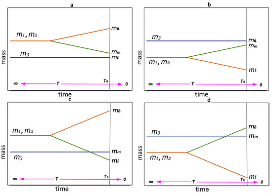
Figure 1. Four scenarios showing how two initially degenerate eigenvalues ($m_1=m_2$) split as parameter $\gamma$ increases from zero, plotted against temperature T (where $T\to \infty$ at the beginning of the universe, $T_0$ is the present temperature, and $T\to 0$ as the universe expands). The scenarios are grouped by initial mass hierarchy: Group A where $m_2=m_1\ge m_3$ (a,c) and Group B where $m_3\ge m_2=m_1$ (b,d). Within each group, splitting occurs in two ways: Type I where $m_1$ and $m_2$ diverge but maintain the original mass ordering (a,b), and Type II where one degenerate mass crosses $m_3$, creating a new hierarchy (c,d). The $m_3$ trajectories are schematic illustrations since parameter $\beta$ also vary with temperature.

In Figure 1, the evolution of fermion masses shows that the relative relationships among the three-generation fermion masses may change throughout cosmic evolution. For example, when two originally degenerate generations of particles (such as $m_1$ and $m_2$) just begin to split, they are very close to each other. However, as $\mathbf{C}$ (or $\gamma$) increases, the two masses gradually diverge, and one of them may gradually approach $m_3$. In this case, the original normal ordering (inverted ordering) would transform into the opposite inverted ordering (normal ordering). It is even possible that the mass hierarchy of all three generations of fermions could change. These issues will be discussed in detail in Section 2.

According to Big Bang cosmology, the universe’s temperature was extremely high in its earliest moments. Since higher temperatures generally correspond to greater symmetry, it is reasonable to infer that the primordial universe was so hot that all symmetries were conserved. As the universe expanded and cooled, these symmetries broke one after another. For instance, spontaneous symmetry breaking (SSB) of electroweak gauge symmetry occurred at approximately 159.5 GeV [40], generating particle masses. Under such conditions, assuming only three fermion generations, an $S_3$ symmetry among them could have existed in the very early universe.

Our previous CPVSM studies revealed a direct connection between CP violation and $S_N$ symmetry breaking. When fermion ${\mathbf{M}}^{\mathbf{2}}$ matrices in weak interactions respect $S_3$ symmetry, CP symmetry remains conserved. However, when $S_3$ symmetry breaks down to $S_2$ symmetry for particular fermion types, complex phases appear in the CKM matrix. As $S_2$ symmetries further break into completely asymmetric structures, both magnitudes and phases of CKM elements vary with the parameters $\alpha$, $\beta$, and $\gamma$. Thus, CPV emerges and evolves alongside $S_N$ symmetry breaking.

Notably, whether the system exhibits $S_N$ symmetry or complete asymmetry, the three mass eigenvalues can remain non-degenerate. Eigenvalue degeneracy depends solely on whether $\gamma =0$, indicating that mass degeneracy is independent of $S_N$ symmetry. These topics will also be explored in detail in Section 2.

Section 3 is devoted to the analysis of neutrino masses and leptogenesis. At the beginning, two neutrino mass ratios are introduced to streamline the subsequent analysis: $g\equiv m_h/m_m$ and $g’\equiv m_m/m_l$. Then, in Section 3.1, all six possible correspondences between the experimentally established ${\Delta }_a$ and ${\Delta }_b$, and the theoretically derived ${\Delta }_{hm}$, ${\Delta }_{ml}$, and ${\Delta }_{hl}$ are systematically examined. Since ${\Delta }_{hm},{\Delta }_{ml}$, and ${\Delta }_{hl}$ are defined to be non-negative, any assignment resulting in a negative MSD is inherently inconsistent. Consequently, four of the six configurations are found to be logically self-consistent, while the remaining two ($\mathbf{Cases}\mathbf{3}$ and $\mathbf{6}$) are excluded.

The analysis then focuses on the four viable cases. $\mathbf{Cases}\mathbf{1}$ and $\mathbf{5}$, grouped as Class 1, both yield the hierarchy $m_h^2\sim m_m^2\gg m_l^2$, indicating that the heavier masses $m_h^2$ and $m_m^2$ are closer to each other and well separated from $m_l^2$. This configuration is usually referred to as inverted ordering (IO). In contrast, $\mathbf{Cases}\mathbf{2}$ and $\mathbf{4}$, designated as Class 2, produce the hierarchy $m_h^2\gg m_m^2\sim m_l^2$, showing that the two lighter masses $m_m^2$ and $m_l^2$ are closer to each other and distant from $m_h^2$. This configuration is usually referred to as normal ordering (NO). Following this approach, we categorize the four viable cases into two classes.

In Class 1 ($\mathbf{Cases}\mathbf{1}$ and $\mathbf{5}$), $m_m^2\sim m_h^2$, while $m_l^2$ is much smaller than both and is therefore assumed to be negligible. As a result, ${\Delta }_a$ is close in value to both $m_m^2$ and $m_h^2$, and may lie between them. Since the exact position of ${\Delta }_a$ is unknown, we adopt the midpoint ${\Delta }_a=(m_h^2+m_m^2)/2$ as a reference to compute the individual neutrino masses and the parameters g and $g’$. The results obtained using this approximation are expected to remain close to the true values. Both cases yield $m_h$ = $5.04688\times {10}^{-2}$ eV and $m_m$ = $4.97283\times {10}^{-2}$ eV. However, $\mathbf{Cases}\mathbf{5}$ results in $m_l$ = 6.09098$i\times {10}^{-3}$ eV, an unphysical imaginary value, indicating that the underlying assumption is not valid in $\mathbf{Case}\mathbf{5}$.

For Class 2 ($\mathbf{Cases}\mathbf{2}$ and $\mathbf{4}$), $m_m^2\sim m_l^2$, and both are much smaller than $m_h^2$. Therefore, we take the midpoint ${\Delta }_b=(m_l^2+m_m^2)/2$ as the reference point. Upon substitution, the two cases differ only slightly in the value of $m_h$: $5.04688\times {10}^{-2}$ eV in $\mathbf{Cases}\mathbf{2}$ and $5.11968\times {10}^{-2}$ eV in $\mathbf{Case}\mathbf{4}$. In contrast, both cases yield identical values of $m_m=1.05499\times {10}^{-2}$ eV and $m_l=6.09098\times {10}^{-3}$ eV.

In scenarios with limited experimental input, a common phenomenological approach involves selecting representative values within the theoretically allowed parameter space to facilitate further analysis. For instance, in Class 1, we impose $({\Delta }_h+{\Delta }_m)/2={\Delta }_a$, while in Class 2, the condition $({\Delta }_m+{\Delta }_l)/2={\Delta }_b$ is adopted. Under these respective assumptions, the predicted values for the intermediate neutrino mass $m_m$ are $4.97283\times {10}^{-2}$ eV in Class 1 and $1.05499\times {10}^{-2}$ eV in Class 2.

Remarkably, three of the four phenomenologically viable configurations–$\mathbf{Cases}\mathbf{1},\mathbf{2}$, and $\mathbf{4}$–yield a consistent prediction for the lightest neutrino mass, $m_l=6.09098\times {10}^{-3}$ eV. In contrast, $\mathbf{Case}\mathbf{5}$ results in a purely imaginary $m_l$, with the same absolute value. This predicted value of $m_l$ is somewhat lower than the global fit estimate $m_1=8.61\times {10}^{-3}$ eV, as reported in [34]—a discrepancy that remains to be tested by future experimental data.

This point-wise trial-and-error method is inherently limited and may overlook viable solutions; it is thus best regarded as a preliminary approach in the absence of stronger constraints. In contrast, Section 3.3 adopts a more systematic analysis by treating g as a continuous variable, thereby providing broader coverage and a more complete picture than the discrete method used in Section 3.1.

In Section 3.2, using the determined neutrino mass parameters, we analyze the mass hierarchies across the four fermion types and compute the twelve corresponding MSDs. The resulting neutrino mass ratios are found to be significantly smaller than those in the other three fermion sectors. Substituting the twelve MSDs into the Jarlskog measure of CPV (as defined in Equation (3)), we find that the product of the two MSD products in the quark sector exceeds that of the lepton sector by approximately 74 orders of magnitude. This suggests that leptogenesis driven by Dirac neutrinos and charged leptons is negligible in the present universe compared to baryogenesis from the quark sector. Even after accounting for the leptonic Jarlskog invariant $J_{\left(l\right)}$, the disparity remains larger than 71 orders of magnitude.

In Section 3.3, neutrino masses are examined from an alternative perspective, yielding results that closely corroborate those presented in Section 3.1. For each scenario considered, analytical expressions are derived to illustrate how $m_h$, $m_m$, $m_l$, and $g^{\prime }$ depend on the scaling factor g.

Among the four cases studied, in $\mathbf{Cases}\mathbf{1}$ and $\mathbf{5}$, $g^{\prime }$ increases from 1 and diverges to infinity as g approaches critical values of 1.014512 and 1.01467, respectively. Similarly, in $\mathbf{Cases}\mathbf{2}$ and $\mathbf{4}$, $g^{\prime }$ also increases from 1 and diverges as g approaches 5.81614 and 5.90148, respectively. Beyond these critical thresholds, the emergence of negative or imaginary mass values imposes physical constraints, limiting the viable parameter space.

Consequently, the neutrino masses are constrained to lie within narrow, well-defined ranges of g, offering potential guidance for the design of future experimental searches. The detailed behaviors of $m_h$, $m_m$, $m_l$, and $g^{\prime }$ as functions of g are plotted and discussed in Section 3.3.

Section 4 is dedicated to conclusions and discussions.

2. Eigenvalue Degeneracy in the CPVSM and Its Extensions

In this section, we briefly review the CP-violating Standard Model (CPVSM) along with some supplementary insights. This top-down approach begins with the most general structure of fermion mass matrices, M, and establishes a mathematical relationship between M and its square, ${\mathbf{M}}^{\mathbf{2}}\equiv M·M^{†}$. A key insight is that both matrices are diagonalized by the same unitary matrix, $\mathbf{U}$. Since ${\mathbf{M}}^{\mathbf{2}}$ is naturally Hermitian, the complexity of the problem is significantly reduced: ${\mathbf{M}}^{\mathbf{2}}$ involves only nine parameters, compared to the eighteen real parameters required for the general complex matrix M.

In top-down models, various assumptions (such as texture zeros) or symmetries (such as discrete flavor symmetries $S_N$, $Z_N$, supersymmetry, etc.) are often introduced to simplify the construction of mass matrices. However, since the actual empirical matrices do not possess these idealized symmetries, the resulting M and $\mathbf{U}$ matrices become overly constrained and fail to reproduce the experimental values.

Our previous research on CP violation in the quark sector demonstrated that lower symmetry leads to better agreement between theoretical predictions and experimental data. This relationship manifests clearly in the behavior of mass eigenvalues and CKM matrix elements. For instance, in $S_N$ symmetric models with $N=3$, the CKM matrix contains only real elements, resulting in complete CP conservation [41]. When $N=2$, the CKM matrix can accommodate complex phases, indicating CP symmetry breaking, though the matrix elements still deviate significantly from experimental values [2,3]. In contrast, when the mass matrix M possesses no imposed symmetry, the resulting CKM matrix elements can reproduce experimental values to $O\left({10}^{-2}\right)$ accuracy [4] at tree level.

The absence of artificial symmetries represents the true situation in our universe. This progression illustrates a fundamental principle in top-down model building: the more restrictive the imposed assumptions and constraints, the greater the deviation from physical reality. Such behavior is both expected and instructive for theoretical construction.

During this process, we encountered a fundamental dilemma: excessive assumptions (i.e., overly strong constraints) cause the structure of M to become oversimplified and detached from reality, while reducing assumptions makes the structure of M too complex to be analytically diagonalizable. Ultimately, we systematically weakened the symmetry of M from $S_3$ and $S_2$ symmetric forms to a completely asymmetric structure. In the following, we briefly introduce these results and extend them to the lepton sector to study CP violation in Dirac neutrinos and their contribution to the baryon asymmetry of the universe (BAU).

As mentioned in the first paragraph of this section, even when M is fully asymmetric, the ${\mathbf{M}}^{\mathbf{2}}$ matrix is necessarily Hermitian and thus contains only nine independent parameters. However, even such a nine-parameter ${\mathbf{M}}^{\mathbf{2}}$ matrix remains too complex for direct analytical diagonalization. Therefore, we introduced the assumption that the real and imaginary parts of ${\mathbf{M}}^{\mathbf{2}}$ can be simultaneously diagonalized by the same unitary matrix $\mathbf{U}$. This is the only simplifying assumption employed throughout our entire investigation and reduces the number of independent parameters to five. Crucially, such a five-parameter matrix is analytically diagonalizable.

As the ${\mathbf{M}}^{\mathbf{2}}$ matrix becomes analytically diagonalizable, both the eigenvalues and the $\mathbf{U}$ matrix can be explicitly derived, and a complex phase naturally emerges in the resulting CKM matrix [3,4]. This provides a specific solution to the problem of the origin of CP violation in the Standard Model, though the framework remains incomplete. Therefore, it is natural to extend this approach to the lepton sector to investigate whether a similar mechanism could generate CP violation in neutrino oscillations. Furthermore, this extension opens the possibility of exploring how leptogenesis might contribute to the observed baryon asymmetry of the universe.

As shown in [2,3,4], the most general $3\times 3$ mass matrix can be expressed as

$$\begin{array}{ccc}\hfill M& =& \left(\begin{array}{ccc}{A}_1+i{D}_1& B_1+i{C}_1& B_2+i{C}_2\\ B_4+i{C}_4& A_2+i{D}_2& B_3+i{C}_3\\ B_5+i{C}_5& B_6+i{C}_6& A_3+i{D}_3\end{array}\right)\hfill \\ & =& M_R+i{M}_I=\left(\begin{array}{ccc}{A}_1& B_1& B_2\\ B_4& A_2& B_3\\ B_5& B_6& A_3\end{array}\right)+i\left(\begin{array}{ccc}{D}_1& C_1& C_2\\ C_4& D_2& C_3\\ C_5& C_6& D_3\end{array}\right),\hfill \end{array}$$

(5)

where there are eighteen independent parameters in total: nine real coefficients and nine imaginary coefficients from the matrix elements. This general form is clearly too complex for analytical diagonalization.

However, the eigenvectors of the M matrix (or, equivalently, the unitary matrix that diagonalizes the M matrix) are identical to those of the mass-squared matrix ${\mathbf{M}}^{\mathbf{2}}\equiv M·M^{†}$. The general form of ${\mathbf{M}}^{\mathbf{2}}$ is given by

$$\begin{array}{ccc}\hfill {\mathbf{M}}^{\mathbf{2}}& =& \left(\begin{array}{ccc}{\mathbf{A}}_{\mathbf{1}}& {\mathbf{B}}_{\mathbf{1}}+\mathbf{i}{\mathbf{C}}_{\mathbf{1}}& {\mathbf{B}}_{\mathbf{2}}+\mathbf{i}{\mathbf{C}}_{\mathbf{2}}\\ {\mathbf{B}}_{\mathbf{1}}-\mathbf{i}{\mathbf{C}}_{\mathbf{1}}& {\mathbf{A}}_{\mathbf{2}}& {\mathbf{B}}_{\mathbf{3}}+\mathbf{i}{\mathbf{C}}_{\mathbf{3}}\\ {\mathbf{B}}_{\mathbf{2}}-\mathbf{i}{\mathbf{C}}_{\mathbf{2}}& {\mathbf{B}}_{\mathbf{3}}-\mathbf{i}{\mathbf{C}}_{\mathbf{3}}& {\mathbf{A}}_{\mathbf{3}}\end{array}\right)\hfill \\ & =& {\mathbf{M}}_{\mathbf{R}}^{\mathbf{2}}+i{\mathbf{M}}_{\mathbf{I}}^{\mathbf{2}}=\left(\begin{array}{ccc}{\mathbf{A}}_{\mathbf{1}}& {\mathbf{B}}_{\mathbf{1}}& {\mathbf{B}}_{\mathbf{2}}\\ {\mathbf{B}}_{\mathbf{1}}& {\mathbf{A}}_{\mathbf{2}}& {\mathbf{B}}_{\mathbf{3}}\\ {\mathbf{B}}_{\mathbf{2}}& {\mathbf{B}}_{\mathbf{3}}& {\mathbf{A}}_{\mathbf{3}}\end{array}\right)+i\left(\begin{array}{ccc}0& {\mathbf{C}}_{\mathbf{1}}& {\mathbf{C}}_{\mathbf{2}}\\ -{\mathbf{C}}_{\mathbf{1}}& 0& {\mathbf{C}}_{\mathbf{3}}\\ -{\mathbf{C}}_{\mathbf{2}}& -{\mathbf{C}}_{\mathbf{3}}& 0\end{array}\right),\hfill \end{array}$$

(6)

where the boldface parameters $\mathbf{A}$, $\mathbf{B}$, and $\mathbf{C}$ are composite functions of the original parameters in M:

$$\begin{array}{ccc}\hfill {\mathbf{A}}_{\mathbf{1}}& =& A_1^2+D_1^2+B_1^2+C_1^2+B_2^2+C_2^2,\hfill \end{array}$$

(7)

$$\begin{array}{ccc}\hfill {\mathbf{A}}_{\mathbf{2}}& =& A_2^2+D_2^2+B_3^2+C_3^2+B_4^2+C_4^2,\hfill \end{array}$$

(8)

$$\begin{array}{ccc}\hfill {\mathbf{A}}_{\mathbf{3}}& =& A_3^2+D_3^2+B_5^2+C_5^2+B_6^2+C_6^2,\hfill \end{array}$$

(9)

$$\begin{array}{ccc}\hfill {\mathbf{B}}_{\mathbf{1}}& =& A_1{B}_4+D_1{C}_4+B_1{A}_2+C_1{D}_2+B_2{B}_3+C_2{C}_3,\hfill \end{array}$$

(10)

$$\begin{array}{ccc}\hfill {\mathbf{B}}_{\mathbf{2}}& =& A_1{B}_5+D_1{C}_5+B_1{B}_6+C_1{C}_6+B_2{A}_3+C_2{D}_3,\hfill \end{array}$$

(11)

$$\begin{array}{ccc}\hfill {\mathbf{B}}_{\mathbf{3}}& =& B_4{B}_5+C_4{C}_5+B_6{A}_2+C_6{D}_2+A_3{B}_3+D_3{C}_3,\hfill \end{array}$$

(12)

$$\begin{array}{ccc}\hfill {\mathbf{C}}_{\mathbf{1}}& =& D_1{B}_4-A_1{C}_4+A_2{C}_1-B_1{D}_2+B_3{C}_2-B_2{C}_3,\hfill \end{array}$$

(13)

$$\begin{array}{ccc}\hfill {\mathbf{C}}_{\mathbf{2}}& =& D_1{B}_5-A_1{C}_5+B_6{C}_1-B_1{C}_6+A_3{C}_2-B_2{D}_3,\hfill \end{array}$$

(14)

$$\begin{array}{ccc}\hfill {\mathbf{C}}_{\mathbf{3}}& =& C_4{B}_5-B_4{C}_5+D_2{B}_6-A_2{C}_6+A_3{C}_3-B_3{D}_3.\hfill \end{array}$$

(15)

The Hermitian structure of ${\mathbf{M}}^{\mathbf{2}}$ (guaranteed by its construction as $M·M^{†}$) ensures that only nine real parameters remain independent: the three real diagonal elements ${\mathbf{A}}_{\mathbf{1}}$, ${\mathbf{A}}_{\mathbf{2}}$, ${\mathbf{A}}_{\mathbf{3}}$, the three real parts of the off-diagonal elements ${\mathbf{B}}_{\mathbf{1}}$, ${\mathbf{B}}_{\mathbf{2}}$, ${\mathbf{B}}_{\mathbf{3}}$, and the three imaginary parts ${\mathbf{C}}_{\mathbf{1}}$, ${\mathbf{C}}_{\mathbf{2}}$, and ${\mathbf{C}}_{\mathbf{3}}$ (which form an antisymmetric matrix). This represents a reduction from the original eighteen parameters in the general non-Hermitian matrix M.

Clearly, diagonalizing the nine-parameter ${\mathbf{M}}^{\mathbf{2}}$ matrix analytically remains impractical due to the complexity of solving the characteristic polynomial of a general $3\times 3$ matrix. However, as demonstrated in [3], if we assume that both the real and imaginary parts ${\mathbf{M}}_{\mathbf{R}}^{\mathbf{2}}$ and ${\mathbf{M}}_{\mathbf{I}}^{\mathbf{2}}$ can be simultaneously diagonalized by the same unitary matrix $\mathbf{U}$, four additional constraints emerge among the nine parameters. This assumption reduces the number of independent parameters from nine to five, making analytical diagonalization feasible.

While this approach yields an analytic solution, it necessarily sacrifices generality by imposing the simultaneous diagonalizability constraint. The assumption requires that ${\mathbf{M}}_{\mathbf{R}}^{\mathbf{2}}$ and ${\mathbf{M}}_{\mathbf{I}}^{\mathbf{2}}$ commute (i.e., $[{\mathbf{M}}_{\mathbf{R}}^{\mathbf{2}},{\mathbf{M}}_{\mathbf{I}}^{\mathbf{2}}]=\mathbf{0}$), which is a non-trivial restriction on the parameter space. Nevertheless, this constraint represents the weakest assumption currently known that enables analytical treatment while preserving physical relevance in neutrino mass matrix studies.

Defining $\mathbf{A}\equiv {\mathbf{A}}_{\mathbf{3}}$, $\mathbf{B}\equiv {\mathbf{B}}_{\mathbf{3}}$, $\mathbf{C}\equiv {\mathbf{C}}_{\mathbf{3}}$, $\mathbf{x}\equiv {\displaystyle \frac{{\mathbf{B}}_{\mathbf{2}}}{{\mathbf{B}}_{\mathbf{3}}}}$, and $\mathbf{y}\equiv {\displaystyle \frac{{\mathbf{B}}_{\mathbf{1}}}{{\mathbf{B}}_{\mathbf{3}}}}$ as the five remaining free parameters and expressing all other parameters in terms of these, the eigenvalues are given by:

$$\begin{array}{ccc}\hfill {\mathbf{m}}_{\mathbf{1}}^{\mathbf{2}}& =& (\mathbf{A}-{\displaystyle \frac{\mathbf{x}}{\mathbf{y}}}\mathbf{B})-{\displaystyle \frac{\sqrt{{\mathbf{x}}^{\mathbf{2}}+{\mathbf{y}}^{\mathbf{2}}+{\mathbf{x}}^{\mathbf{2}}{\mathbf{y}}^{\mathbf{2}}}}{\mathbf{x}\mathbf{y}}}\mathbf{C},\hfill \end{array}$$

(16)

$$\begin{array}{ccc}\hfill {\mathbf{m}}_{\mathbf{2}}^{\mathbf{2}}& =& (\mathbf{A}-{\displaystyle \frac{\mathbf{x}}{\mathbf{y}}}\mathbf{B})+{\displaystyle \frac{\sqrt{{\mathbf{x}}^{\mathbf{2}}+{\mathbf{y}}^{\mathbf{2}}+{\mathbf{x}}^{\mathbf{2}}{\mathbf{y}}^{\mathbf{2}}}}{\mathbf{x}\mathbf{y}}}\mathbf{C},\hfill \end{array}$$

(17)

$$\begin{array}{ccc}\hfill {\mathbf{m}}_{\mathbf{3}}^{\mathbf{2}}& =& \mathbf{A}+{\displaystyle \frac{({\mathbf{x}}^{\mathbf{2}}+\mathbf{1})\mathbf{y}}{\mathbf{x}}}\mathbf{B}\hfill \\ & =& (\mathbf{A}-{\displaystyle \frac{\mathbf{x}}{\mathbf{y}}}\mathbf{B})+{\displaystyle \frac{{\mathbf{x}}^{\mathbf{2}}{\mathbf{y}}^{\mathbf{2}}+{\mathbf{x}}^{\mathbf{2}}+{\mathbf{y}}^{\mathbf{2}}}{\mathbf{x}\mathbf{y}}}\mathbf{B},\hfill \end{array}$$

(18)

where we introduce the convenient notation $\sigma \equiv \sqrt{{\mathbf{x}}^2+{\mathbf{y}}^2}$ and $\rho \equiv \sqrt{{\mathbf{x}}^2+{\mathbf{y}}^2+{\mathbf{x}}^2{\mathbf{y}}^2}$ to simplify the expressions.

The corresponding unitary matrix $\mathbf{U}$ that diagonalizes ${\mathbf{M}}^{\mathbf{2}}$ is:

$$\begin{array}{ccc}\hfill \mathbf{U}& =& {\displaystyle \frac{1}{\sqrt{2}}}\left(\begin{array}{ccc}{\displaystyle \frac{-\sigma }{\rho }}& {\displaystyle \frac{\mathbf{x}({\mathbf{y}}^2-i\rho )}{\sigma \rho }}& {\displaystyle \frac{\mathbf{y}({\mathbf{x}}^2+i\rho )}{\sigma \rho }}\\ {\displaystyle \frac{-\sigma }{\rho }}& {\displaystyle \frac{\mathbf{x}({\mathbf{y}}^2+i\rho )}{\sigma \rho }}& {\displaystyle \frac{\mathbf{y}({\mathbf{x}}^2-i\rho )}{\sigma \rho }}\\ {\displaystyle \frac{\sqrt{2}\mathbf{x}\mathbf{y}}{\rho }}& {\displaystyle \frac{\sqrt{2}\mathbf{y}}{\rho }}& {\displaystyle \frac{\sqrt{2}\mathbf{x}}{\rho }}\end{array}\right)\hfill \\ & =& \left(\begin{array}{ccc}{\displaystyle \frac{-\sqrt{{\mathbf{x}}^{\mathbf{2}}+{\mathbf{y}}^{\mathbf{2}}}}{\sqrt{\mathbf{2}({\mathbf{x}}^{\mathbf{2}}+{\mathbf{y}}^{\mathbf{2}}+{\mathbf{x}}^{\mathbf{2}}{\mathbf{y}}^{\mathbf{2}})}}}& {\displaystyle \frac{\mathbf{x}({\mathbf{y}}^{\mathbf{2}}-\mathbf{i}\sqrt{{\mathbf{x}}^{\mathbf{2}}+{\mathbf{y}}^{\mathbf{2}}+{\mathbf{x}}^{\mathbf{2}}{\mathbf{y}}^{\mathbf{2}}})}{\sqrt{\mathbf{2}}\sqrt{{\mathbf{x}}^{\mathbf{2}}+{\mathbf{y}}^{\mathbf{2}}}\sqrt{{\mathbf{x}}^{\mathbf{2}}+{\mathbf{y}}^{\mathbf{2}}+{\mathbf{x}}^{\mathbf{2}}{\mathbf{y}}^{\mathbf{2}}}}}& {\displaystyle \frac{\mathbf{y}({\mathbf{x}}^{\mathbf{2}}+\mathbf{i}\sqrt{{\mathbf{x}}^{\mathbf{2}}+{\mathbf{y}}^{\mathbf{2}}+{\mathbf{x}}^{\mathbf{2}}{\mathbf{y}}^{\mathbf{2}}})}{\sqrt{\mathbf{2}}\sqrt{{\mathbf{x}}^{\mathbf{2}}+{\mathbf{y}}^{\mathbf{2}}}\sqrt{{\mathbf{x}}^{\mathbf{2}}+{\mathbf{y}}^{\mathbf{2}}+{\mathbf{x}}^{\mathbf{2}}{\mathbf{y}}^{\mathbf{2}}}}}\\ {\displaystyle \frac{-\sqrt{{\mathbf{x}}^{\mathbf{2}}+{\mathbf{y}}^{\mathbf{2}}}}{\sqrt{\mathbf{2}({\mathbf{x}}^{\mathbf{2}}+{\mathbf{y}}^{\mathbf{2}}+{\mathbf{x}}^{\mathbf{2}}{\mathbf{y}}^{\mathbf{2}})}}}& {\displaystyle \frac{\mathbf{x}({\mathbf{y}}^{\mathbf{2}}+\mathbf{i}\sqrt{{\mathbf{x}}^{\mathbf{2}}+{\mathbf{y}}^{\mathbf{2}}+{\mathbf{x}}^{\mathbf{2}}{\mathbf{y}}^{\mathbf{2}}})}{\sqrt{\mathbf{2}}\sqrt{{\mathbf{x}}^{\mathbf{2}}+{\mathbf{y}}^{\mathbf{2}}}\sqrt{{\mathbf{x}}^{\mathbf{2}}+{\mathbf{y}}^{\mathbf{2}}+{\mathbf{x}}^{\mathbf{2}}{\mathbf{y}}^{\mathbf{2}}}}}& {\displaystyle \frac{\mathbf{y}({\mathbf{x}}^{\mathbf{2}}-\mathbf{i}\sqrt{{\mathbf{x}}^{\mathbf{2}}+{\mathbf{y}}^{\mathbf{2}}+{\mathbf{x}}^{\mathbf{2}}{\mathbf{y}}^{\mathbf{2}}})}{\sqrt{\mathbf{2}}\sqrt{{\mathbf{x}}^{\mathbf{2}}+{\mathbf{y}}^{\mathbf{2}}}\sqrt{{\mathbf{x}}^{\mathbf{2}}+{\mathbf{y}}^{\mathbf{2}}+{\mathbf{x}}^{\mathbf{2}}{\mathbf{y}}^{\mathbf{2}}}}}\\ {\displaystyle \frac{\mathbf{x}\mathbf{y}}{\sqrt{{\mathbf{x}}^{\mathbf{2}}+{\mathbf{y}}^{\mathbf{2}}+{\mathbf{x}}^{\mathbf{2}}{\mathbf{y}}^{\mathbf{2}}}}}& {\displaystyle \frac{\mathbf{y}}{\sqrt{{\mathbf{x}}^{\mathbf{2}}+{\mathbf{y}}^{\mathbf{2}}+{\mathbf{x}}^{\mathbf{2}}{\mathbf{y}}^{\mathbf{2}}}}}& {\displaystyle \frac{\mathbf{x}}{\sqrt{{\mathbf{x}}^{\mathbf{2}}+{\mathbf{y}}^{\mathbf{2}}+{\mathbf{x}}^{\mathbf{2}}{\mathbf{y}}^{\mathbf{2}}}}}\end{array}\right).\hfill \end{array}$$

(19)

Notably, in such a model, the $\mathbf{U}$ matrix depends on only two of the five remaining parameters ($\mathbf{x}$ and $\mathbf{y}$), while being independent of the other three ($\mathbf{A}$, $\mathbf{B}$, and $\mathbf{C}$). This remarkable feature significantly simplifies the diagonalization procedure and provides insight into the structure of the mass matrix.

It should be emphasized that the mass-squared eigenvalues ${\mathbf{m}}_{\mathbf{1}}^{\mathbf{2}}$, ${\mathbf{m}}_{\mathbf{2}}^{\mathbf{2}}$, and ${\mathbf{m}}_{\mathbf{3}}^{\mathbf{2}}$ may correspond to the physical fermion masses in various ways. As previously noted, the heaviest, intermediate, and lightest fermions of a given type are denoted by $m_h$, $m_m$, and $m_l$, respectively. Since the eigenvalues can be ordered differently depending on the parameter values, all possible permutations relating the three eigenvalues to the three physical masses must be systematically investigated to ensure complete coverage of the parameter space.

In such a parameterization, the ${\mathbf{M}}^{\mathbf{2}}$ matrix can be explicitly expressed as

$$\begin{array}{ccc}\hfill {\mathbf{M}}^{\mathbf{2}}& =& \left(\begin{array}{ccc}\mathbf{A}+(\mathbf{x}\mathbf{y}-{\displaystyle \frac{\mathbf{x}}{\mathbf{y}}})\mathbf{B}& \mathbf{y}\mathbf{B}& \mathbf{x}\mathbf{B}\\ \mathbf{y}\mathbf{B}& \mathbf{A}+({\displaystyle \frac{\mathbf{y}}{\mathbf{x}}}-{\displaystyle \frac{\mathbf{x}}{\mathbf{y}}})\mathbf{B}& \mathbf{B}\\ \mathbf{x}\mathbf{B}& \mathbf{B}& \mathbf{A}\end{array}\right)\hfill \\ & +& i\left(\begin{array}{ccc}0& {\displaystyle \frac{\mathbf{1}}{\mathbf{y}}}\mathbf{C}& -{\displaystyle \frac{\mathbf{1}}{\mathbf{x}}}\mathbf{C}\\ -{\displaystyle \frac{\mathbf{1}}{\mathbf{y}}}\mathbf{C}& 0& \mathbf{C}\\ {\displaystyle \frac{\mathbf{1}}{\mathbf{x}}}\mathbf{C}& -\mathbf{C}& 0\end{array}\right).\hfill \end{array}$$

(20)

In Equations (16)–(18), there are five free parameters appearing in the three eigenvalue expressions, but only three measured masses are available for each fermion type. Thus, it is clearly impossible to determine all parameters uniquely from the mass data alone.

However, we can establish a more direct connection between theory and experiment by introducing three physically meaningful combinations. Let us define $\alpha$ as the $\mathbf{A}$- and $\mathbf{B}$-dependent terms in the leading brackets of Equations (16)–(18), $\gamma$ as the $\mathbf{C}$-dependent terms, and $\beta \equiv {\mathbf{m}}_{\mathbf{3}}^{\mathbf{2}}-\alpha$. The eigenvalues can then be rewritten in the simplified form:

$$\begin{array}{ccc}\hfill {\mathbf{m}}_{\mathbf{1}}^{\mathbf{2}}=\alpha -\gamma ,{\mathbf{m}}_{\mathbf{2}}^{\mathbf{2}}& =& \alpha +\gamma ,{\mathbf{m}}_{\mathbf{3}}^{\mathbf{2}}=\alpha +\beta ,\hfill \end{array}$$

(21)

with the useful relation:

$$\begin{array}{c}\hfill {\mathbf{m}}_{\mathbf{1}}^{\mathbf{2}}+{\mathbf{m}}_{\mathbf{2}}^{\mathbf{2}}+{\mathbf{m}}_{\mathbf{3}}^{\mathbf{2}}=3\alpha +\beta .\end{array}$$

(22)

The parameters $\alpha$, $\beta$, and $\gamma$ can be calculated directly from the measured masses:

$$\begin{array}{ccc}\hfill \alpha & =& {\displaystyle \frac{({\mathbf{m}}_{\mathbf{1}}^{\mathbf{2}}+{\mathbf{m}}_{\mathbf{2}}^{\mathbf{2}})}{\mathbf{2}}}=\mathbf{A}-{\displaystyle \frac{\mathbf{x}}{\mathbf{y}}}\mathbf{B},\hfill \end{array}$$

(23)

$$\begin{array}{ccc}\hfill \beta & =& {\mathbf{m}}_{\mathbf{3}}^{\mathbf{2}}-{\displaystyle \frac{({\mathbf{m}}_{\mathbf{1}}^{\mathbf{2}}+{\mathbf{m}}_{\mathbf{2}}^{\mathbf{2}})}{\mathbf{2}}}={\displaystyle \frac{({\mathbf{x}}^{\mathbf{2}}{\mathbf{y}}^{\mathbf{2}}+{\mathbf{x}}^{\mathbf{2}}+{\mathbf{y}}^{\mathbf{2}})}{\mathbf{x}\mathbf{y}}}\mathbf{B},\hfill \end{array}$$

(24)

$$\begin{array}{ccc}\hfill \gamma & =& {\displaystyle \frac{({\mathbf{m}}_{\mathbf{2}}^{\mathbf{2}}-{\mathbf{m}}_{\mathbf{1}}^{\mathbf{2}})}{\mathbf{2}}}={\displaystyle \frac{\sqrt{{\mathbf{x}}^{\mathbf{2}}+{\mathbf{y}}^{\mathbf{2}}+{\mathbf{x}}^{\mathbf{2}}{\mathbf{y}}^{\mathbf{2}}}}{\mathbf{x}\mathbf{y}}}\mathsf{C}.\hfill \end{array}$$

(25)

These three quantities establish a direct connection between the theoretical framework ($\alpha$, $\beta$, $\gamma$) and experimental data (${\mathbf{m}}_{\mathbf{1}}^{\mathbf{2}},{\mathbf{m}}_{\mathbf{2}}^{\mathbf{2}},{\mathbf{m}}_{\mathbf{3}}^{\mathbf{2}}$). While $\alpha$, $\beta$, and $\gamma$ themselves depend on the five underlying parameters ($\mathbf{A},\mathbf{B},\mathbf{C},\mathbf{x},\mathbf{y}$) through Equations (21) and (22), their values are experimentally determined, providing three constraints that reduce but do not eliminate the parameter space.

This approach obviously applies to the quark sector and charged leptons and potentially to Dirac neutrinos as well. Such a simplification will be helpful in the coming analyses to be shown below.

In Equation (22), it is evident that the sum of the three mass-squares depends only on the parameters $\alpha$ and $\beta$. The variation of $\gamma$, if it does vary, does not affect the sum of the three mass-squares for a given fermion type. Interestingly, two of the eigenvalues become degenerate when $\mathbf{C}$ = 0 (which makes $\gamma =0$), with splitting occurring only when $\gamma$ becomes non-trivial.

It is evident from Equation (25) that the first term of $\gamma$ satisfies ${\displaystyle \frac{\sqrt{x^2+y^2+x^2{y}^2}}{xy}}>1$ for arbitrary values of $\mathbf{x}$ and $\mathbf{y}$. This inequality implies that $\gamma$ vanishes if and only if $\mathbf{C}=\mathbf{0}$. Therefore, non-zero $\mathbf{C}$ leads to eigenvalue splitting, lifting the degeneracy. However, the underlying mechanism responsible for generating a non-trivial $\mathbf{C}$ remains unclear. It is plausible that this mechanism is related to the temperature of the universe, as many physical phenomena exhibit symmetry breaking below certain critical temperature thresholds.

Regardless of how the eigenvalues lose their degeneracy, the evolution pattern is constrained by the initial configuration ($\gamma =0$) and subsequent splitting dynamics. This yields four possible scenarios, as illustrated in Figure 1, which shows the evolution of the eigenvalues with temperature. These configurations can be categorized into two distinct groups, which represent limiting cases that occur when $\gamma$ = 0—that is, before full mass splitting:

Group 1: $m_2=m_1>m_3$ (Figure 1a,c)

Group 2: $m_3>m_2=m_1$ (Figure 1b,d)

Within each group, there are two distinct ways in which the initially degenerate states can further split:

(i) In one scenario, $m_1$ and $m_2$ split, and one of them evolves to surpass $m_3$; this can occur whether the initially degenerate pair lies above (Figure 1c) or below (Figure 1d) $m_3$.

(ii) In the other scenario, $m_1$ and $m_2$ split but remain on the same side of $m_3$, never intersecting its trajectory (Figure 1a,b).

In this way, the parameters $\alpha$, $\beta$, and $\gamma$ can be determined unambiguously by substituting experimentally measured fermion masses into Equations (23)–(25). For example, when applied to the charged lepton sector, the input values are $m_l=m_e$ = 0.000511 GeV, $m_m=m_{\mu }$ = 0.1057 GeV, and $m_h=m_{\tau }$ = 1.7768 GeV. However, there are six distinct ways to assign the eigenvalues $m_1^2$, $m_2^2$, and $m_3^2$ to the physical squared masses $m_l^2$, $m_m^2$, and $m_h^2$, as listed below:

$$\begin{array}{ccc}\hfill \mathrm{Case}\mathrm{A}.(m_1^2,m_2^2,m_3^2)& \to & (m_l^2,m_m^2,m_h^2),\hfill \end{array}$$

(26)

$$\begin{array}{ccc}\hfill \mathrm{Case}\mathrm{B}.(m_1^2,m_2^2,m_3^2)& \to & (m_l^2,m_h^2,m_m^2),\hfill \end{array}$$

(27)

$$\begin{array}{ccc}\hfill \mathrm{Case}\mathrm{C}.(m_1^2,m_2^2,m_3^2)& \to & (m_m^2,m_l^2,m_h^2),\hfill \end{array}$$

(28)

$$\begin{array}{ccc}\hfill \mathrm{Case}\mathrm{D}.(m_1^2,m_2^2,m_3^2)& \to & (m_m^2,m_h^2,m_l^2),\hfill \end{array}$$

(29)

$$\begin{array}{ccc}\hfill \mathrm{Case}\mathrm{E}.(m_1^2,m_2^2,m_3^2)& \to & (m_h^2,m_m^2,m_l^2),\hfill \end{array}$$

(30)

$$\begin{array}{ccc}\hfill \mathrm{Case}\mathrm{F}.(m_1^2,m_2^2,m_3^2)& \to & (m_h^2,m_l^2,m_m^2),\hfill \end{array}$$

(31)

Each of these cases will be discussed in detail in the following analysis.

2.1. $(m_1^2,m_2^2,m_3^2)\to (m_l^2,m_m^2,m_h^2)$

Taking the charged leptons as an example, $m_l=m_e$ = 0.000511 GeV, $m_m=m_{\mu }$= 0.1057 GeV, and $m_h=m_{\tau }$ = 1.7768 GeV. In this case

$$\begin{array}{ccc}\hfill {\alpha }_{\mathcal{l}1}& =& {\displaystyle \frac{m_{\mu }^2+m_e^2}{2}}=5.58638\times {10}^{-3}{\mathrm{GeV}}^2,\hfill \end{array}$$

(32)

$$\begin{array}{ccc}\hfill {\beta }_{\mathcal{l}1}& =& m_{\tau }^2-{\alpha }_{\mathcal{l}1}={\displaystyle \frac{({{\mathbf{x}}^{\mathbf{2}}}_{\mathcal{l}}{{\mathbf{y}}^{\mathbf{2}}}_{\mathcal{l}}+{{\mathbf{x}}^{\mathbf{2}}}_{\mathcal{l}}+{{\mathbf{y}}^{\mathbf{2}}}_{\mathcal{l}})}{{\mathbf{x}}_{\mathcal{l}}{\mathbf{y}}_{\mathcal{l}}}}{\mathbf{B}}_{\mathcal{l}}=3.15214{\mathrm{GeV}}^2,\hfill \end{array}$$

(33)

$$\begin{array}{ccc}\hfill {\gamma }_{\mathcal{l}1}& =& {\displaystyle \frac{m_{\mu }^2-m_e^2}{2}}={\displaystyle \frac{\sqrt{{{\mathbf{x}}^{\mathbf{2}}}_{\mathcal{l}}+{{\mathbf{y}}^{\mathbf{2}}}_{\mathcal{l}}+{{\mathbf{x}}^{\mathbf{2}}}_{\mathcal{l}}{{\mathbf{y}}^{\mathbf{2}}}_{\mathcal{l}}}}{{\mathbf{x}}_{\mathcal{l}}{\mathbf{y}}_{\mathcal{l}}}}{\mathbf{C}}_{\mathcal{l}}=5.58611\times {10}^{-3}{\mathrm{GeV}}^2,\hfill \end{array}$$

(34)

where the subscript ℓ denotes charged leptons. Note that while $\alpha$, $\beta$, and $\gamma$ are now determined from the measured masses, the underlying parameters ${\mathbf{A}}_{\mathcal{l}}$, ${\mathbf{B}}_{\mathcal{l}}$, ${\mathbf{C}}_{\mathcal{l}}$, ${\mathbf{x}}_{\mathcal{l}}$, and ${\mathbf{y}}_{\mathcal{l}}$ remain undetermined—a situation common to all six cases.

2.2. $(m_1^2,m_2^2,m_3^2)\to (m_l^2,m_h^2,m_m^2)$

$$\begin{array}{ccc}\hfill {\alpha }_{\mathcal{l}2}& =& {\displaystyle \frac{m_{\tau }^2+m_e^2}{2}}=1.57886{\mathrm{GeV}}^2,\hfill \end{array}$$

(35)

$$\begin{array}{ccc}\hfill {\beta }_{\mathcal{l}2}& =& m_{\mu }^2-{\alpha }_{\mathcal{l}2}=-1.56769{\mathrm{GeV}}^2,\hfill \end{array}$$

(36)

$$\begin{array}{ccc}\hfill {\gamma }_{\mathcal{l}2}& =& {\displaystyle \frac{m_{\tau }^2-m_e^2}{2}}=1.57886{\mathrm{GeV}}^2.\hfill \end{array}$$

(37)

2.3. $(m_1^2,m_2^2,m_3^2)\to (m_m^2,m_l^2,m_h^2)$

$$\begin{array}{ccc}\hfill {\alpha }_{\mathcal{l}3}& =& {\displaystyle \frac{m_e^2+m_{\mu }^2}{2}}=5.58638\times {10}^{-3}{\mathrm{GeV}}^2,\hfill \end{array}$$

(38)

$$\begin{array}{ccc}\hfill {\beta }_{\mathcal{l}3}& =& m_{\tau }^2-{\alpha }_{\mathcal{l}3}=3.15214{\mathrm{GeV}}^2,\hfill \end{array}$$

(39)

$$\begin{array}{ccc}\hfill {\gamma }_{\mathcal{l}3}& =& {\displaystyle \frac{m_e^2-m_{\mu }^2}{2}}=-5.58611\times {10}^{-3}{\mathrm{GeV}}^2.\hfill \end{array}$$

(40)

2.4. $(m_1^2,m_2^2,m_3^2)\to (m_m^2,m_h^2,m_l^2)$

$$\begin{array}{ccc}\hfill {\alpha }_{\mathcal{l}4}& =& {\displaystyle \frac{m_{\tau }^2+m_{\mu }^2}{2}}=1.58445{\mathrm{GeV}}^2,\hfill \end{array}$$

(41)

$$\begin{array}{ccc}\hfill {\beta }_{\mathcal{l}4}& =& m_e^2-{\alpha }_{\mathcal{l}4}=-1.58445{\mathrm{GeV}}^2,\hfill \end{array}$$

(42)

$$\begin{array}{ccc}\hfill {\gamma }_{\mathcal{l}4}& =& {\displaystyle \frac{m_{\tau }^2-m_{\mu }^2}{2}}=1.57328{\mathrm{GeV}}^2.\hfill \end{array}$$

(43)

2.5. $(m_1^2,m_2^2,m_3^2)\to (m_h^2,m_m^2,m_l^2)$

$$\begin{array}{ccc}\hfill {\alpha }_{\mathcal{l}5}& =& {\displaystyle \frac{m_{\mu }^2+m_{\tau }^2}{2}}=1.58445{\mathrm{GeV}}^2,\hfill \end{array}$$

(44)

$$\begin{array}{ccc}\hfill {\beta }_{\mathcal{l}5}& =& m_e^2-{\alpha }_{\mathcal{l}5}=-1.58445{\mathrm{GeV}}^2,\hfill \end{array}$$

(45)

$$\begin{array}{ccc}\hfill {\gamma }_{\mathcal{l}5}& =& {\displaystyle \frac{m_{\mu }^2-m_{\tau }^2}{2}}=-1.57328{\mathrm{GeV}}^2.\hfill \end{array}$$

(46)

2.6. $(m_1^2,m_2^2,m_3^2)\to (m_h^2,m_l^2,m_m^2)$

$$\begin{array}{ccc}\hfill {\alpha }_{\mathcal{l}6}& =& {\displaystyle \frac{m_e^2+m_{\tau }^2}{2}}=1.57886{\mathrm{GeV}}^2,\hfill \end{array}$$

(47)

$$\begin{array}{ccc}\hfill {\beta }_{\mathcal{l}6}& =& m_{\mu }^2-{\alpha }_{\mathcal{l}6}=-1.56769{\mathrm{GeV}}^2,\hfill \end{array}$$

(48)

$$\begin{array}{ccc}\hfill {\gamma }_{\mathcal{l}6}& =& {\displaystyle \frac{m_e^2-m_{\tau }^2}{2}}=-1.57886{\mathrm{GeV}}^2.\hfill \end{array}$$

(49)

Similarly, the $\alpha$, $\beta$, and $\gamma$ parameters for other fermion types can be determined in the same manner. For instance, these parameters for the charged leptons, up-type quarks, and down-type quarks are provided in Table 1, Table 2, and Table 3, respectively. Note that in Cases C, E, and F, the negative values of $\gamma$ indicate a reversed mass ordering between $m_1$ and $m_2$ relative to the positive-$\gamma$ cases. In the next section, we will also examine these parameters in the neutrino sector.

Although the parameters $\mathbf{A}$, $\mathbf{B}$, $\mathbf{C}$, $\mathbf{x}$, and $\mathbf{y}$ are not conclusively determined by the fermion masses at this stage, the parameters $\alpha$, $\beta$, and $\gamma$ are fixed. These parameters exhibit a degeneracy between two of the three eigenvalues when $\mathbf{C}=0$, and an even more pronounced degeneracy involving all three generations when $\beta =\gamma =0$, resulting in ${\mathbf{m}}_{\mathbf{1}}^{\mathbf{2}}={\mathbf{m}}_{\mathbf{2}}^{\mathbf{2}}={\mathbf{m}}_{\mathbf{3}}^{\mathbf{2}}=\alpha$. The evolution of $\gamma$ and $\beta$ (and consequently the eigenvalues) with temperature or cosmological time could be of significant interest and warrants further investigation.

3. Neutrino Masses and Leptogenesis

In the earliest development of the electroweak Standard Model, neutrinos were assumed to be massless particles. Moreover, since they are the only neutral fermions, they could potentially differ from the other three types of Dirac fermions and might be Majorana particles. Consequently, many behaviors or characteristics that exist in other fermion sectors cannot be directly extended to the neutrino sector.

When neutrino oscillation experiments confirmed that neutrinos have mass, the Standard Model required important modifications. First, neutrino mass terms must be added to the Lagrangian and a mass matrix must be constructed. Second, it must be determined whether they are Dirac particles or Majorana particles, since the mass generation mechanisms for these two cases are fundamentally different—if neutrinos are Majorana particles, their mass terms would violate lepton number conservation and require physics beyond the minimal Standard Model.

Furthermore, generating neutrino masses in a way consistent with their observed smallness poses a theoretical challenge. If one introduces right-handed neutrinos to enable Dirac mass terms via the Higgs mechanism, additional mechanisms such as the seesaw are typically invoked to explain why neutrino masses are orders of magnitude smaller than other fermion masses. Alternatively, Majorana mass terms can be generated through higher-dimensional operators, which also require physics beyond the Standard Model.

It should be noted that in the CPVSM framework, we approach our research from the perspective of how a general mass matrix M can be diagonalized. Although the mass generation in our discussion proceeds through the Higgs mechanism, the mathematical formalism does not inherently restrict it to this source alone. Even if other mass terms, such as Majorana-type contributions, are discovered in the future, the matrix diagonalization methodology presented here represents fundamental mathematics that will equally apply to those cases.

For consistency with our treatment of quarks and charged leptons in the CPVSM framework, and to establish a baseline analysis using the same diagonalization formalism, this work treats neutrinos as Dirac particles. We recognize that Majorana neutrinos remain a viable and important possibility; investigating CP violation in a Majorana framework would require modifications to the mass matrix structure and represents a natural extension of this work.

Among the four fermion sectors in the Standard Model, three—up-type quarks, down-type quarks, and charged leptons—have experimentally well-determined masses. However, for neutrinos, only two mass-squared differences (MSDs) are currently measured, making it impossible to determine the absolute values of the three neutrino masses. This section presents a detailed investigation of the neutrino sector, aimed at constraining the possible mass ranges of the three neutrino mass eigenstates within our theoretical framework.

We establish notational conventions to streamline the subsequent analysis. As previously defined, we denote the masses of the heaviest, intermediate, and lightest fermions of a given type are denoted by $m_h$, $m_m$, and $m_l$, respectively. To facilitate the calculations, we introduce two dimensionless mass ratios:

$$\begin{array}{ccc}\hfill g& =& m_h/m_m(\mathrm{heavy}-\mathrm{to}-\mathrm{medium}\mathrm{ratio}),\hfill \\ \hfill g^{\prime }& =& m_m/m_l(\mathrm{medium}-\mathrm{to}-\mathrm{light}\mathrm{ratio}),\hfill \end{array}$$

(50)

where g and $g^{\prime }$ are positive parameters that quantify the mass hierarchies between successive states. These ratios will prove instrumental in the phenomenological analysis that follows.

3.1. Analysis of Neutrino Mass-Squared Differences

The two experimentally obtained MSDs are denoted as

$$\begin{array}{c}\hfill {\Delta }_a=2.51\times {10}^{-3}{\mathrm{eV}}^2\mathrm{and}{\Delta }_b=7.42\times {10}^{-5}{\mathrm{eV}}^2.\end{array}$$

(51)

The three theoretical defined MSDs are expressed as ${\Delta }_{hm}=(m_h^2-m_m^2)\ge 0$, ${\Delta }_{hl}=(m_h^2-m_l^2)\ge 0$, and ${\Delta }_{ml}=(m_m^2-m_l^2)\ge 0$, all of which are non-negative by definition. These quantities satisfy the relation ${\Delta }_{hm}+{\Delta }_{ml}={\Delta }_{hl}$, as stated in Equation (2).

There are six possible correspondences between the experimental MSDs, ${\Delta }_a$ and ${\Delta }_b$, and the three theoretical MSDs, ${\Delta }_{hl}$, ${\Delta }_{ml}$, and ${\Delta }_{hm}$, as outlined below:

$\mathbf{Case}\mathbf{1}$: ${\Delta }_{hl}\iff {\Delta }_a$ and ${\Delta }_{hm}\iff {\Delta }_b$. Then ${\Delta }_{ml}={\Delta }_a-{\Delta }_b>0$.

$\mathbf{Case}\mathbf{2}$: ${\Delta }_{hl}\iff {\Delta }_a$ and ${\Delta }_{ml}\iff {\Delta }_b$. Then ${\Delta }_{hm}={\Delta }_a-{\Delta }_b>0$.

$\mathbf{Case}\mathbf{3}$: ${\Delta }_{hm}\iff {\Delta }_a$ and ${\Delta }_{hl}\iff {\Delta }_b$. This case is excluded since it would imply ${\Delta }_{hm}={\Delta }_b-{\Delta }_a<0$, contradicting the definition given above.

$\mathbf{Case}\mathbf{4}$: ${\Delta }_{hm}\iff {\Delta }_a$ and ${\Delta }_{ml}\iff {\Delta }_b$. Then ${\Delta }_{hl}={\Delta }_a+{\Delta }_b>0$.

$\mathbf{Case}\mathbf{5}$: ${\Delta }_{ml}\iff {\Delta }_a$ and ${\Delta }_{hm}\iff {\Delta }_b$. Then ${\Delta }_{hl}={\Delta }_a+{\Delta }_b>0$.

$\mathbf{Case}\mathbf{6}$: ${\Delta }_{ml}\iff {\Delta }_a$ and ${\Delta }_{hl}\iff {\Delta }_b$. This case is excluded since it would imply ${\Delta }_{hm}={\Delta }_b-{\Delta }_a<0$, contradicting the definition given above.

Among these, $\mathbf{Cases}\mathbf{3}\mathrm{and}\mathbf{6}$ are excluded based on the non-negativity constraints and the relation ${\Delta }_{hm}+{\Delta }_{ml}={\Delta }_{hl}$. We now proceed to analyze the remaining four viable cases individually, as follows.

Case 1

In this case, we set ${\Delta }_{hl}={\Delta }_a$ and ${\Delta }_{hm}={\Delta }_b$. This yields:

$$\begin{array}{c}\hfill {\Delta }_{ml}={\Delta }_a-{\Delta }_b=2.4358\times {10}^{-3}{\mathrm{eV}}^2.\end{array}$$

(52)

The resulting hierarchy is ${\Delta }_{hl}\sim {\Delta }_{ml}\gg {\Delta }_{hm}$, or equivalently, $m_h^2\sim m_m^2\gg m_l^2$. This mass pattern corresponds to the inverted ordering (IO) by definition.

Since $m_h^2-m_l^2={\Delta }_a\approx m_m^2-m_l^2$ and assuming $m_l^2$ is negligible compared to $m_h^2$ and $m_m^2$, it follows that ${\Delta }_a$ must be approximately equal to both $m_h^2$ and $m_m^2$. Therefore, we can reasonably approximate ${\Delta }_a$ as the midpoint between these two values: $(m_h^2+m_m^2)/2\approx {\Delta }_a$. Under this assumption, the predicted neutrino masses should closely match their actual values.

Combining the midpoint approximation $(m_h^2+m_m^2)/2\approx {\Delta }_a$ with the difference $(m_h^2-m_m^2)={\Delta }_b$, we obtain:

$$\begin{array}{ccc}\hfill m_h& =& 5.04688\times {10}^{-2}\mathrm{eV},m_m=4.97283\times {10}^{-2}\mathrm{eV},\hfill \\ \hfill m_l& =& 6.09098\times {10}^{-3}\mathrm{eV},g=1.01489,\hfill \\ \hfill g^{\prime }& =& 8.16425,g·g^{\prime }=8.28583.\hfill \end{array}$$

(53)

The mass ratios $g\sim 1$ and $g^{\prime }\gg 1$ are consistent with the inverted ordering constraint $m_h\sim m_m\gg m_l$.

Case 2

In this case, let ${\Delta }_{hl}={\Delta }_a$ and ${\Delta }_{ml}={\Delta }_b$. Then

$$\begin{array}{c}\hfill {\Delta }_{hm}={\Delta }_a-{\Delta }_b=2.4358\times {10}^{-3}{\mathrm{eV}}^2.\end{array}$$

(54)

This indicates that ${\Delta }_{hl}\sim {\Delta }_{hm}\gg {\Delta }_{ml}$, or equivalently, $m_h^2\gg m_m^2\sim m_l^2$. This is the normal ordering (NO) by definition.

Following a similar approach as in $\mathbf{Case}\mathbf{1}$, let ${\Delta }_b$ be the midpoint between $m_m^2$ and $m_l^2$, i.e., $(m_m^2+m_l^2)/2\approx {\Delta }_b$. Combining this with $(m_m^2-m_l^2)={\Delta }_b$, we obtain:

$$\begin{array}{ccc}\hfill m_h& =& 5.04688\times {10}^{-2}\mathrm{eV},m_m=1.05499\times {10}^{-2}\mathrm{eV},\hfill \\ \hfill m_l& =& 6.09098\times {10}^{-3}\mathrm{eV},g=4.78383,\hfill \\ \hfill g^{\prime }& =& 1.73205,g·g^{\prime }=8.28583.\hfill \end{array}$$

(55)

The ratios g and $g^{\prime }$ do not align well with the expected mass hierarchy $m_h\gg m_m\sim m_l$. In particular, they are significantly smaller than those observed in the other three fermion types, and the value $g^{\prime }=1.73205$ suggests that $m_m$ is not particularly close to $m_l$.

Case 4

In this case, let ${\Delta }_{hm}={\Delta }_a$ and ${\Delta }_{ml}={\Delta }_b$. Then

$$\begin{array}{c}\hfill {\Delta }_{hl}={\Delta }_a+{\Delta }_b=2.5842\times {10}^{-3}{\mathrm{eV}}^2.\end{array}$$

(56)

This indicates ${\Delta }_{hl}\sim {\Delta }_{hm}\gg {\Delta }_{ml}$, or equivalently, $m_h^2\gg m_m^2\sim m_l^2$, similar to $\mathbf{Case}\mathbf{2}$. This is also the normal ordering (NO) by definition.

Following the same approach as in $\mathbf{Case}\mathbf{2}$, let ${\Delta }_b$ be the midpoint between $m_m^2$ and $m_l^2$, i.e., $(m_m^2+m_l^2)/2\approx {\Delta }_b$. Combining this with $(m_m^2-m_l^2)={\Delta }_b$, we obtain:

$$\begin{array}{ccc}\hfill m_h& =& 5.11968\times {10}^{-2}\mathrm{eV},m_m=1.05499\times {10}^{-2}\mathrm{eV},\hfill \\ \hfill m_l& =& 6.09098\times {10}^{-3}\mathrm{eV},g=4.85301,\hfill \\ \hfill g^{\prime }& =& 1.73205,g·g^{\prime }=8.405.\hfill \end{array}$$

(57)

The masses of the lighter two neutrinos are identical to those in $\mathbf{Case}\mathbf{2}$; however, the heavier mass is slightly larger, with $m_h=5.11968\times {10}^{-2}$ eV.

Case 5

In this case, let ${\Delta }_{ml}={\Delta }_a$ and ${\Delta }_{hm}={\Delta }_b$. Then

$$\begin{array}{c}\hfill {\Delta }_{hl}={\Delta }_a+{\Delta }_b=2.5842\times {10}^{-3}{\mathrm{eV}}^2.\end{array}$$

(58)

This indicates ${\Delta }_{ml}\sim {\Delta }_{hl}\gg {\Delta }_{hm}$, or $m_h^2\sim m_m^2\gg m_l^2$, similar to $\mathbf{Case}\mathbf{1}$. This is also the inverted ordering (IO) by definition.

Following the same considerations as in $\mathbf{Case}\mathbf{1}$, ${\Delta }_a$ is treated as the midpoint between $m_h^2$ and $m_m^2$, i.e., $(m_h^2+m_m^2)/2\approx {\Delta }_a$. Combining this with $(m_h^2-m_m^2)={\Delta }_b$, we obtain:

$$\begin{array}{ccc}\hfill m_h& =& 5.04688\times {10}^{-2}\mathrm{eV},m_m=4.97283\times {10}^{-2}\mathrm{eV},\hfill \\ \hfill m_l& =& 6.09098i\times {10}^{-3}\mathrm{eV},g=1.01489,\hfill \\ \hfill g^{\prime }& =& 8.16425i,g·g^{\prime }=8.28583i.\hfill \end{array}$$

(59)

The results obtained here are similar to those in $\mathbf{Case}\mathbf{1}$, except that $m_l$ is imaginary, which is unphysical. This indicates that the assumption ${\displaystyle \frac{m_h^2+m_m^2}{2}}\approx {\Delta }_a$ must be rejected for this case. However, it lies close to the boundary of the physically allowed region, as will be confirmed through an alternative analytical approach in Section 3.3 and visualized in Figure 9.

As a summary, the predicted value of $m_l\approx 6.09098\times {10}^{-3}$ eV remains across three of the four cases. This value differs from the naive estimate $m_1\approx \sqrt{{\Delta }_b}=8.61\times {10}^{-3}$ eV, which would be obtained by assuming $m_2\gg m_1$ and neglecting $m_1^2$ in ${\Delta }_b=m_2^2-m_1^2$ [34]. Alongside the earlier prediction of $m_3=5.01\times {10}^{-2}$ eV, we now also predict various values for $m_h$ and the intermediate mass $m_m$.

There are primarily two groups of predictions for $m_m$: one suggests $m_m\approx 4.97283\times {10}^{-2}$ eV, assumed to be closer to $m_h$, while the other proposes $m_m\approx 1.05499\times {10}^{-2}$ eV, assumed to be closer to $m_l$. In either case, the neutrino mass ratios are significantly smaller compared to those of the other three fermion types. The details are summarized in Table 4.

Table 4. Case 5 yields an imaginary value for $m_l$, making it unphysical and excluding it from further consideration. The remaining three cases are noteworthy for future investigations.

$\mathbf{Case}$	${\mathit{m}}_{\mathit{h}}\left(\mathbf{eV}\right)$	${\mathit{m}}_{\mathit{m}}\left(\mathbf{eV}\right)$	${\mathit{m}}_{\mathit{l}}\left(\mathbf{eV}\right)$	g	${\mathit{g}}^{\prime }$	$\mathbf{Physical}$
$\begin{array}{c}\mathbf{1}\\ \mathbf{5}\\ \mathbf{2}\\ \mathbf{4}\end{array}$	$\begin{array}{c}5.05\times {10}^{-2}\\ 5.05\times {10}^{-2}\\ 5.05\times {10}^{-2}\\ 5.12\times {10}^{-2}\end{array}$	$\begin{array}{c}4.97\times {10}^{-2}\\ 4.97\times {10}^{-2}\\ 1.05\times {10}^{-2}\\ 1.05\times {10}^{-2}\end{array}$	$\begin{array}{c}6.09\times {10}^{-3}\\ 6.09i\times {10}^{-3}\\ 6.09\times {10}^{-3}\\ 6.09\times {10}^{-3}\end{array}$	$\begin{array}{c}1.01\\ 1.01\\ 4.78\\ 4.85\end{array}$	$\begin{array}{c}8.16\\ 8.16i\\ 1.73\\ 1.73\end{array}$	$\begin{array}{c}\mathrm{Yes}\\ \mathrm{No}\\ \mathrm{Possibly}\\ \mathrm{Possibly}\end{array}$

In $\mathbf{Cases}\mathbf{1}\mathrm{and}\mathbf{5}$ (IO), where $g=1.01489$, this ratio suggests that $m_h\approx m_m$, and the value ${\Delta }_a=2.51\times {10}^{-3}$ eV² may represent a combination of ${\Delta }_{hl}$ and ${\Delta }_{ml}$. If this interpretation is correct, future experiments with improved precision could potentially resolve the difference between these two MSDs. The predicted values presented here may serve as a useful reference for guiding the design of such experiments.

In contrast, for the other group (NO) with $g^{\prime }\approx 1.73205$, the difference between $m_m$ and $m_l$ is substantial, making them easier to distinguish compared to the previous group. While this scenario is mathematically viable, the relatively small mass ratio $g^{\prime }\approx 1.73$ differs notably from the hierarchical patterns seen in other fermion sectors, making it a less natural prediction within our framework.

3.2. Mass Hierarchy, Leptonic CP Violation and Leptogenesis

Among the four fermion types in the Standard Model, three sectors—up-type quarks, down-type quarks, and charged leptons—each contain three generations whose masses are well established experimentally. For neutrinos, considering only their Dirac component, only two mass-squared differences (MSDs) have been measured experimentally, rather than the three absolute masses that would fully characterize the sector.

The third neutrino MSD can be determined from the two experimental values using the constraint Equations (1) or (2). However, ambiguity arises because there are four viable ways to pair the three theoretical mass-squared differences ${\Delta }_{ij}$ with the two experimental values ${\Delta }_{(a,b)}$. This yields four candidate sets of twelve MSDs across all fermion sectors, which can be used to calculate the Jarlskog measure of CP violation in both quark and lepton sectors—corresponding to baryogenesis and leptogenesis processes, respectively—allowing us to compare their contributions to the observed baryon asymmetry of the universe.

Investigation of all four candidate pairings yields nearly identical conclusions: leptogenesis from Dirac neutrinos is at least 71 orders of magnitude weaker than baryogenesis in the current universe, even accounting for Jarlskog invariants in both quark and lepton sectors. However, within the Standard Model and its minimal extension with sterile right-handed neutrinos, there exists the potential for leptogenesis to dominate over baryogenesis during certain critical phases of $S_N$ flavor symmetry breaking in the primordial universe.

We substitute the nine well-established fermion masses and the three predicted neutrino masses into Equation (50) to estimate mass hierarchies across different fermion types and generations. This analysis reveals that mass ratios in the neutrino sector are much smaller than those in the other three fermion sectors. Especially in $\mathbf{Cases}\mathbf{1}$ and $\mathbf{5}$, the two heavier neutrino generations are nearly degenerate.

The analysis of mass ratios across the three charged fermion sectors follows:

• 1. For up-type quarks

$$\begin{array}{ccc}\hfill g_{\left(u\right)}& \equiv & {\displaystyle \frac{m_t}{m_c}}>{\displaystyle \frac{(172.0-0.9-1.3)}{(1.27+0.07)}}\sim 126.7,\hfill \\ \hfill g_{\left(u\right)}^{\prime }& \equiv & {\displaystyle \frac{m_c}{m_u}}>{\displaystyle \frac{(1.27-0.09)}{0.0033}}\sim 357.6.\hfill \end{array}$$

(60)

• 2. For down-type quarks

$$\begin{array}{ccc}\hfill g_{\left(d\right)}& \equiv & {\displaystyle \frac{m_b}{m_s}}>{\displaystyle \frac{(4.19-0.06)}{(0.101+0.029)}}\sim 31.77,\hfill \\ \hfill g_{\left(d\right)}^{\prime }& \equiv & {\displaystyle \frac{m_s}{m_d}}>{\displaystyle \frac{(0.101-0.021)}{0.0058}}\sim 13.79.\hfill \end{array}$$

(61)

• 3. For charged leptons

$$\begin{array}{ccc}\hfill g_{\left(\mathcal{l}\right)}& & {\displaystyle \frac{m_{\tau }}{m_{\mu }}}>{\displaystyle \frac{1777}{105.7}}\sim 16.81,\hfill \\ \hfill g_{\left(\mathcal{l}\right)}^{\prime }& \equiv & {\displaystyle \frac{m_{\mu }}{m_e}}>{\displaystyle \frac{105.7}{0.511}}\sim 206.8.\hfill \end{array}$$

(62)

Note: In the equations above, the maximum of the masses in the denominator and the minimum in the numerator are chosen to ensure the “>” signs always hold true. Among these six ratios, the smallest one is $g_{\left(d\right)}^{\prime }\approx 13.79$. This value is much larger than the comparable ratios obtained for neutrinos, as shown below.

• 4. For neutrinos

The candidate ratio sets are:

$\mathbf{Case}\mathbf{1}$, $g_{\left(\nu \right)}=1.01489$, $g_{\left(\nu \right)}^{\prime }=8.16425$, and $g_{\left(\nu \right)}·g_{\left(\nu \right)}^{\prime }=8.28583$.

$\mathbf{Case}\mathbf{2}$, $g_{\left(\nu \right)}=4.78383$, $g_{\left(\nu \right)}^{\prime }=1.73205$, and $g_{\left(\nu \right)}·g_{\left(\nu \right)}^{\prime }=8.28583$.

$\mathbf{Case}\mathbf{4}$, $g_{\left(\nu \right)}=4.85301$, $g_{\left(\nu \right)}^{\prime }=1.73205$, and $g_{\left(\nu \right)}·g_{\left(\nu \right)}^{\prime }=8.40500$.

Considering the mass ratios in the quark sector and in charged leptons, $g_{\left(d\right)}^{\prime }\equiv {\displaystyle \frac{m_s}{m_d}}\approx 13.79$ is the smallest among these three fermion types. The difference between $(m_s^2-m_d^2)$ and $m_s^2$ is only about ${\displaystyle \frac{1}{g_{\left(d\right)}^{\prime 2}}}\approx {\displaystyle \frac{1}{190.2}}$ of $m_s^2$. It is therefore reasonable to ignore the mass of the lighter fermion in such a MSD. However, the ratios $g_{\left(\nu \right)}$ and $g_{\left(\nu \right)}^{\prime }$ obtained in Section 3.1 do not justify such approximations in any of the neutrino cases.

In each of the remaining three viable cases, the product $g·g^{\prime }\equiv {\displaystyle \frac{m_h}{m_l}}$ range between 8.28583 and 8.40500, which are significantly smaller than the corresponding ratios in the other three fermion types. These values are clearly too small to disregard any $m_l$ in the subsequent derivations for neutrinos.

In the quark sector, Jarlskog suggested a measure for the strength of CP violation [35]:

$$\begin{array}{ccc}\hfill {\Delta }_{CP}& =& \mathrm{Im}\mathrm{Det}[m_u{m}_u^{†},m_d{m}_d^{†}]T^{-12}\hfill \\ & =& \mathit{J}\prod _{i<j}(m_{u,i}^2-m_{u,j}^2)\prod _{i<j}(m_{d,i}^2-m_{d,j}^2)T^{-12}\hfill \\ & =& \mathit{J}\Delta m_{\left(u\right)}^2\Delta m_{\left(d\right)}^2{T}^{-12},\hfill \end{array}$$

(63)

where J is the Jarlskog invariant, $T\approx$ 100 GeV is the temperature of the electroweak phase transition, and $m^2$ represents squares of quark masses.

In the last line of Equation (63), $\Delta m_{\left(u\right)}^2$ and $\Delta m_{\left(d\right)}^2$ are the products of three MSDs in the up- and down-type quarks, defined as:

$$\begin{array}{ccc}\hfill \Delta m_{\left(u\right)}^2& =& (m_t^2-m_c^2)(m_c^2-m_u^2)(m_u^2-m_t^2)\hfill \end{array}$$

$$\begin{array}{ccc}& =& -(m_t^2-m_c^2)(m_c^2-m_u^2)(m_t^2-m_u^2)<0,\hfill \end{array}$$

(64)

$$\begin{array}{ccc}\hfill \Delta m_{\left(d\right)}^2& =& (m_b^2-m_s^2)(m_s^2-m_d^2)(m_d^2-m_b^2)\hfill \\ & =& -(m_b^2-m_s^2)(m_s^2-m_d^2)(m_b^2-m_d^2)<0,\hfill \end{array}$$

(65)

respectively.

In the lepton sector, the maximally allowed CP-violating Jarlskog invariant was estimated to be [31]:

$$\begin{array}{c}\hfill J_{\left(l\right)}^{max}=0.033\pm 0.010\pm \left(0.027\right).\end{array}$$

(66)

In the expression for CP violation in Equation (63), six MSDs appear in the quark sector: three from up-type quarks and three from down-type quarks. Similarly, there should be three MSDs from charged leptons and three from neutrinos in the lepton sector. From recent global analyses of three-flavor neutrino oscillations, the neutrino MSDs are given by:

$$\begin{array}{ccc}\hfill \Delta m_{31}^2& =& {2.517}_{-0.028}^{+0.026}·{10}^{-3}{\mathrm{eV}}^2,\left(\mathrm{NO}\right)\hfill \end{array}$$

(67)

$$\begin{array}{ccc}\hfill \Delta m_{32}^2& =& -{2.498}_{-0.028}^{+0.026}·{10}^{-3}{\mathrm{eV}}^2,\left(\mathrm{IO}\right)\hfill \end{array}$$

(68)

$$\begin{array}{ccc}\hfill \Delta m_{21}^2& =& {7.42}_{-0.20}^{+0.21}·{10}^{-5}{\mathrm{eV}}^2,\hfill \end{array}$$

(69)

where $\Delta m_{ij}^2=m_i^2-m_j^2$ denotes the MSD between neutrinos i and j, NO (IO) is the abbreviation for Normal ordering (Inverted ordering), defined by $m_3\gg m_2\sim m_1$ ($m_3\sim m_2\gg m_1$) as described in [42]. However, only two of the MSDs are obtained experimentally.

In general, two given values are insufficient to analytically determine three unknowns. However, in the case of mass-squared differences (MSDs), the third MSD can be determined unambiguously due to the constraint:

$$\begin{array}{c}\hfill {\Delta }_{hm}+{\Delta }_{ml}\equiv (m_h^2-m_m^2)+(m_m^2-m_l^2)=(m_h^2-m_l^2)\equiv {\Delta }_{hl}.\end{array}$$

(70)

This identity ensures that any two of the MSDs uniquely determine the third. The remaining question is how the two experimentally measured quantities ${\Delta }_{(a,b)}$ correspond to the three theoretical ${\Delta }_{ij}$.

As discussed in Section 3.1, there are six possible correspondences between ${\Delta }_{(a,b)}$ and ${\Delta }_{ij}$. Among these, only four candidates are logically self-consistent:

• $\mathbf{Case}\mathbf{1}:$ Let ${\Delta }_a={\Delta }_{hl}=(m_h^2-m_l^2)$ and ${\Delta }_b={\Delta }_{hm}=$$(m_h^2-m_m^2)$, then ${\Delta }_{ml}=(m_m^2-m_l^2)={\Delta }_a-{\Delta }_b=2.4358·{10}^{-3}$ eV².

• $\mathbf{Case}\mathbf{2}:$ Let ${\Delta }_a={\Delta }_{hl}=(m_h^2-m_l^2)$ and ${\Delta }_b={\Delta }_{ml}=$$(m_m^2-m_l^2)$, then ${\Delta }_{hm}=(m_h^2-m_m^2)={\Delta }_a-{\Delta }_b=2.4358·{10}^{-3}$ eV².

• $\mathbf{Case}\mathbf{4}:$ Let ${\Delta }_a={\Delta }_{hm}=(m_h^2-m_m^2)$ and ${\Delta }_b={\Delta }_{ml}=$$(m_m^2-m_l^2)$, then ${\Delta }_{hl}=(m_h^2-m_l^2)={\Delta }_a+{\Delta }_b=2.5842·{10}^{-3}$ eV².

• $\mathbf{Case}\mathbf{5}:$ Let ${\Delta }_a={\Delta }_{ml}=(m_m^2-m_l^2)$ and ${\Delta }_b={\Delta }_{hm}=$$(m_h^2-m_m^2)$, then ${\Delta }_{hl}=(m_h^2-m_l^2)={\Delta }_a+{\Delta }_b=2.5842·{10}^{-3}$ eV².

There is a particularly interesting quantity, $\Delta m_{\left(\nu \right)}^2$, the product of three MSDs for neutrinos, defined by:

$$\begin{array}{ccc}\hfill \Delta m_{\left(\nu \right)}^2& \equiv & {(m_h^2-m_m^2)}_{\left(\nu \right)}{(m_m^2-m_l^2)}_{\left(\nu \right)}{(m_l^2-m_h^2)}_{\left(\nu \right)}\hfill \\ & =& {({\Delta }_{hm}·{\Delta }_{ml}·{\Delta }_{lh})}_{\left(\nu \right)}=-2{\gamma }_{\left(\nu \right)}({\beta }_{\left(\nu \right)}^2-{\gamma }_{\left(\nu \right)}^2),\hfill \end{array}$$

(71)

which is almost the same in all cases. Besides, it indicates that $\Delta m_{\left(\nu \right)}^2$ is independent of the parameter ${\alpha }_{\left(\nu \right)}$.

Upon substituting the results obtained in the neutrino sector into Equation (71), the following outcomes are derived:

In Cases 1 and 2:

$$\begin{array}{c}\hfill |\Delta m_{\left(\nu \right)}^2|={\Delta }_a{\Delta }_b({\Delta }_a-{\Delta }_b)=4.8129\times {10}^{-64}{\mathrm{GeV}}^6.\end{array}$$

(72)

In Cases 4 and 5:

$$\begin{array}{c}\hfill |\Delta m_{\left(\nu \right)}^2|={\Delta }_a{\Delta }_b({\Delta }_a+{\Delta }_b)=4.5365\times {10}^{-64}{\mathrm{GeV}}^6.\end{array}$$

(73)

These products of neutrino MSDs are remarkably similar regardless of how ${\Delta }_a$ and ${\Delta }_b$ correspond to the three ${\Delta }_{ij}$. However, the $\Delta m_{\left(\nu \right)}^2$ values are dramatically smaller than the similar quantities in the other three fermion types:

For up-type quarks:

$$\begin{array}{c}\hfill |\Delta m_{\left(u\right)}^2|\approx 1.463\times {10}^9{\mathrm{GeV}}^6,\end{array}$$

(74)

(Using $m_t$ = 173.21 GeV, $m_c$ = 1.275 GeV, and $m_u$ = 0.0023 GeV).

For down-type quarks:

$$\begin{array}{c}\hfill |\Delta m_{\left(d\right)}^2|\approx 2.747{\mathrm{GeV}}^6,\end{array}$$

(75)

(Using $m_b$ = 4.180 GeV, $m_s$ = 0.095 GeV, and $m_d$ = 0.0048 GeV).

For charged leptons:

$$\begin{array}{c}\hfill |\Delta m_{\left(\mathcal{l}\right)}^2|\approx 0.1107{\mathrm{GeV}}^6,\end{array}$$

(76)

(Using $m_{\tau }$ = 1.7768 GeV, $m_{\mu }$ = 0.1056 GeV, and $m_e$ = 0.000511 GeV).

The MSD products for the other three fermion types are at least 62 orders of magnitude larger than that of neutrinos, representing a vast hierarchy that remains an unexplained mystery in physics. By substituting the MSD products for the quark sector into the CPV measure Equation (63), we obtain:

$$\begin{array}{c}\hfill |{\Delta }_{CP\left(q\right)}|\approx J_{\left(q\right)}·4.019\times {10}^9{\mathrm{GeV}}^6{T}^{-12},\end{array}$$

(77)

while for the lepton sector:

$$\begin{array}{c}\hfill \left|{\Delta }_{CP\left(l\right)}\right|\approx J_{\left(l\right)}·{(}_{5.0219}^{5.3279})\times {10}^{-65}{\mathrm{GeV}}^6{T}^{-12}.\end{array}$$

(78)

Taking the Jarlskog invariant in the quark sector as $J_{\left(q\right)}=3.0\times {10}^{-5}$ [43] and the maximally allowed CP-violating Jarlskog invariant in the lepton sector, $J_{\left(l\right)}\approx 0.033$ [31], the CPV measure in the quark sector is still at least 71 orders of magnitude greater than that in the lepton sector. This stark difference in CP violation measures at the electroweak scale suggests that, within the framework of Dirac neutrinos and the minimal Standard Model, leptogenesis contributions would be suppressed by at least 71 orders of magnitude compared to quark-driven baryogenesis. However, this conclusion applies to the low-energy CP violation parameters; a complete assessment of leptogenesis would require analyzing high-temperature dynamics, decay processes, and washout effects in the early universe.

3.3. An Alternative Approach to Studying Neutrino Masses

In this subsection, we employ a different approach from Section 3.1 to study the relationships among the three Dirac neutrino masses. Here we treat the two mass ratios $g’$ and g as continuous variables rather than as discrete test points as in Section 3.1, making the results more complete and reasonable.

First, we replace $m_h$ and $m_m$ with g, $g’$, and $m_l$, then substitute them into ${\Delta }_a$ and ${\Delta }_b$. By using the ratio ${\displaystyle \frac{{\Delta }_a}{{\Delta }_b}}=33.8275$, we completely eliminate $m_l$ to obtain the relationship between $g^{\prime }$ and g. Next, we express $g^{\prime }$ as a function of g. Natural constraints—such as both ratios being positive real numbers greater than or equal to 1—can then be used to strictly limit their possible ranges.

Subsequently, according to the definitions of ${\Delta }_b$ in different cases, substituting $g^{\prime }$ as a function of g allows $m_l$, $m_n$, and $m_h$ to all become functions of the single variable g. Thus, by studying their variation with g, we can determine the mass ratio relationships among the various neutrinos. Interestingly, in all four possible scenarios, when g approaches the test values used in Section 3.1, the lightest neutrino mass consistently converges to $m_l=6.09098\times {10}^{-3}$ eV, which shows significant deviation from the previous prediction of $m_1=8.61\times {10}^{-3}$ eV. These discrepancies are important considerations for future experiments.

We now present the detailed analysis for each case. In $\mathbf{Case}\mathbf{1}$ of Section 3.1, the following relationships hold:

$$\begin{array}{ccc}\hfill {\displaystyle \frac{{\Delta }_a}{{\Delta }_b}}& =& 33.8275={\displaystyle \frac{(g^2{g}^{\prime 2}-1)m_l^2}{(g^2{g}^{\prime 2}-g^{\prime 2})m_l^2}},\hfill \end{array}$$

(79)

$$\begin{array}{ccc}\hfill g^{\prime }& =& \sqrt{{\displaystyle \frac{1}{33.8275-32.8275g^2}}},\hfill \end{array}$$

(80)

$$\begin{array}{ccc}\hfill m_l& =& \sqrt{{\displaystyle \frac{{\Delta }_b}{g^{\prime 2}(g^2-1)}}}.\hfill \end{array}$$

(81)

Figure 2 illustrates the variation of $g^{\prime }$ with respect to g, showing that $g^{\prime }$ increases sharply toward infinity as g approaches 1.01512. This divergence occurs as the denominator of Equation (80) approaches zero.

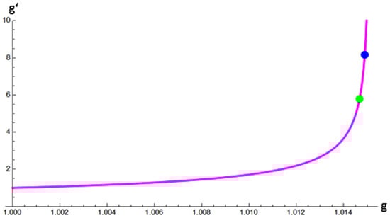
Figure 2. The variation of $g^{\prime }$ with g reveals that $g^{\prime }$ increases sharply toward infinity as g approaches 1.01512. Consequently, the self-consistent range in this case is restricted to a very narrow interval, $1<g<1.01512$. For reference, two points are marked in the figure: the blue point at $(g,g^{\prime })=(1.01489,8.16425)$ represents the result obtained in Equation (53) of Section 3.1, while the green point at $(g,g^{\prime })=(1.01467,5.79514)$ is obtained by substituting the predicted value $m_1=8.61\times {10}^{-3}$ eV from [34] into Equation (81). The region between these two points is an area that future experimental designs should focus on investigating.

Furthermore, Figure 3 presents the variation of $m_h$, $m_m$, and $m_l$ with respect to g. In this figure, when g approaches 1, $m_h\approx m_m\approx m_l$. However, as g increases beyond 1, $m_l$ diverges from the other two and decreases rapidly to zero as g approaches 1.01512. Beyond that point, $m_h$ and $m_m$ become negative and $m_l$ becomes imaginary, which are obviously unphysical.

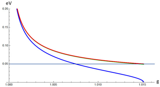
Figure 3. In this figure, the red, green, and blue curves represent the variations of $m_h$, $m_m$, and $m_l$ with respect to g, respectively. These variations reveal that the three neutrino masses are nearly degenerate when g is close to 1, with the red and green curves ($m_h$ and $m_m$) remaining almost overlapping throughout the entire physically allowed range. As g increases toward the critical value of 1.01512, $m_l$ (blue curve) gradually separates from the other two masses and approaches zero, while $m_m$ continues to track closely with $m_h$. Beyond $g=1.01512$, the mass eigenvalues become unphysical, marking the boundary of the physically meaningful parameter space.

Consequently, physically meaningful neutrino masses that satisfy $m_h>m_m>m_l>0$ are only allowed within a very narrow range $1<g<1.01512$. In Figure 2, two reference points are plotted: a blue point at $(g,g^{\prime })=(1.01489,8.16425)$, where $g·g^{\prime }\approx 8.28583$, corresponds to the results obtained in Equation (53); and a green point at $(g,g^{\prime })=(1.01467,5.79514)$, which is obtained by substituting the value $m_1=8.61\times {10}^{-3}$ eV predicted in [34] into Equation (81). With these reference points established, the range between these two points will be a primary focus of our attention in the future.

In $\mathbf{Case}\mathbf{2}$ of Section 3.1, the following relationships are observed:

$$\begin{array}{ccc}\hfill {\displaystyle \frac{{\Delta }_a}{{\Delta }_b}}& =& 33.8275={\displaystyle \frac{(g^2{g}^{\prime 2}-1)m_l^2}{(g^{\prime 2}-1)m_l^2}},\hfill \end{array}$$

(82)

$$\begin{array}{ccc}\hfill g^{\prime }& =& \sqrt{{\displaystyle \frac{32.8275}{33.8275-g^2}}},\hfill \end{array}$$

(83)

$$\begin{array}{ccc}\hfill m_l& =& \sqrt{{\displaystyle \frac{{\Delta }_b}{g^{\prime 2}-1}}}.\hfill \end{array}$$

(84)

Figure 4 illustrates the variation of $g^{\prime }$ with respect to g, showing that $g^{\prime }$ increases sharply toward infinity as g approaches 5.81614. This divergence occurs as the denominator of Equation (83) approaches zero.

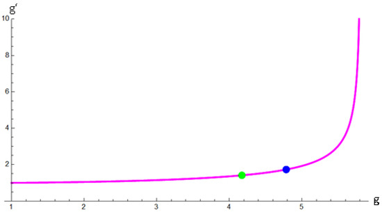
Figure 4. This figure shows that $g^{\prime }$ increases sharply toward infinity as g approaches 5.81614. Consequently, the physically meaningful range for this case lies within $1<g<5.81614$. For reference, two points are marked. The blue point at $(g,g^{\prime })=(4.78383,1.73205)$ represents the result obtained in Equation (55) of Section 3.1, while the green point at $(g,g^{\prime })=(4.17388,1.41454)$ is obtained by substituting the predicted value $m_1=8.61\times {10}^{-3}$ eV from [34] into Equation (84). The region between these two points is an area that future experimental designs should pay closer attention to.

Furthermore, Figure 5 presents the variation of $m_h$, $m_m$, and $m_l$ with respect to g. In this figure, when g approaches 1, we have $m_h\approx m_m\approx m_l$. However, as g increases beyond 1, $m_h$ diverges from the other two. As g further increases, $m_h$ approaches a constant value of approximately $5.01\times {10}^{-2}$ eV. Meanwhile, $m_m$ and $m_l$ remain very close to each other, decreasing gradually until g approaches 5.81614. At this point, where $g^2={\displaystyle \frac{{\Delta }_a}{{\Delta }_b}}$, $m_l$ drops to zero. Beyond that point, unphysical negative and imaginary neutrino masses emerge.

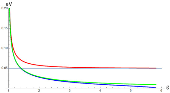
Figure 5. In this figure, the red, green, and blue lines represent the variations of $m_h$, $m_m$, and $m_l$ with respect to g, respectively. These variations show that the three neutrino masses are nearly degenerate when g is close to 1. As g increases, $m_h$ (red line) begins to deviate from the other two masses, while $m_l$ (blue line) approaches zero as g approaches 5.81614. At this critical value, $m_m$ (green line) approaches the constant value $1.055\times {10}^{-2}$ eV, as derived in Section 3.1. Beyond $g=5.81614$, the mass eigenvalues become unphysical, defining the upper boundary of the physically meaningful parameter space.

Consequently, physically meaningful neutrino masses that satisfy $m_h>m_m>m_l>0$ occur only within the range $1<g<5.81614$. In Figure 4, two reference points are plotted: a blue point at $(g,g^{\prime })=(4.78383,1.73205)$, which corresponds to the results from Equation (55) and aligns well with the curve; and a green point at $(g,g^{\prime })=(4.17388,1.41454)$, obtained by substituting the predicted value $m_1=8.61\times {10}^{-3}$ eV from [34] into Equation (84). The range between these two points will be a primary focus of our attention in the future.

In Case 4 of Section 3.1, the following relationships are observed:

$$\begin{array}{ccc}\hfill {\displaystyle \frac{{\Delta }_a}{{\Delta }_b}}& =& 33.8275={\displaystyle \frac{g^{\prime 2}(g^2-1)m_l^2}{(g^{\prime 2}-1)m_l^2}},\hfill \end{array}$$

(85)

$$\begin{array}{ccc}\hfill g^{\prime }& =& \sqrt{{\displaystyle \frac{33.8275}{34.8275-g^2}}},\hfill \end{array}$$

(86)

$$\begin{array}{ccc}\hfill m_l& =& \sqrt{{\displaystyle \frac{{\Delta }_b}{g^{\prime 2}-1}}}.\hfill \end{array}$$

(87)

Figure 6 illustrates the variation of $g^{\prime }$ with respect to g, showing that $g^{\prime }$ increases sharply to infinity as g approaches 5.90148, where the denominator of Equation (86) approaches zero. This critical value is close to the value 5.81614 obtained in Case 2, with both cases exhibiting similar qualitative behavior at large g.

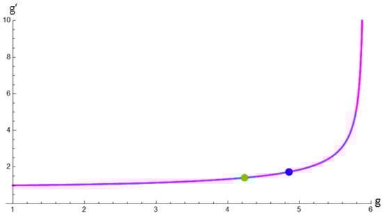
Figure 6. The variation of $g^{\prime }$ with g reveals that $g^{\prime }$ increases sharply towards infinity as g approaches 5.90148. Consequently, the self-consistent range for this case lies within $1<g<5.90148$. For reference, two points are marked in the figure: the blue point at ($g,g^{\prime }$) = (4.85301, 1.73205) represents the result obtained in Equation (57) of Section 3.1, while the green point at ($g,g^{\prime }$) = (4.23338, 1.41454) is obtained by substituting the predicted value $m_1=8.61\times {10}^{-3}$ eV from [34] into Equation (87). The region between these two points represents a key parameter space that future experimental designs should target for investigation.

Furthermore, Figure 7 presents the variation of $m_h$, $m_m$, and $m_l$ with respect to g. In this figure, when g approaches 1, we have $m_h\approx m_m\approx m_l$. However, as g increases beyond 1, $m_h$ diverges from the other two. As g increases further, $m_h$ approaches a constant value of approximately $5.01\times {10}^{-2}$ eV, while $m_m$ and $m_l$ remain very close to each other and decrease slowly until g approaches 5.90148, at which point $g^2={\displaystyle \frac{{\Delta }_a}{{\Delta }_b}}$ and $m_l$ drops to zero sharply. Beyond that point, unphysical negative and imaginary neutrino masses emerge.

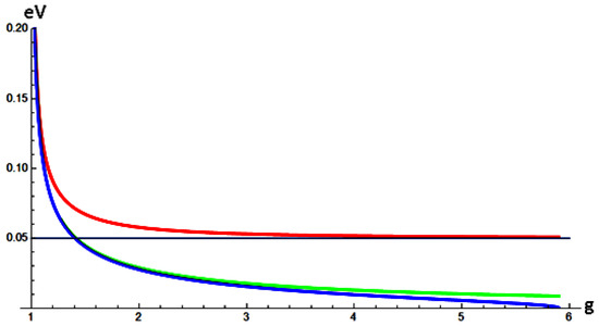
Figure 7. As g increases, $m_h$ (red line) starts to deviate from the other two masses, while $m_l$ (blue line) approaches zero as g approaches the critical value of 5.90148. Meanwhile, $m_m$ (green line) remains relatively stable throughout this range. Beyond $g=5.90148$, the mass eigenvalues become unphysical, marking the boundary of the physically meaningful parameter space.

Consequently, physically meaningful neutrino masses satisfying $m_h>m_m>m_l>0$ occur only within the range $1<g<5.90148$. In Figure 6, two reference points are plotted: a blue point at $(g,g^{\prime })=(4.85301,1.73205)$, which corresponds to the results from Equation (57) and aligns well with the curve; and a green point at $(g,g^{\prime })=(4.23338,1.41454)$, obtained by substituting the predicted value $m_1=8.61\times {10}^{-3}$ eV from [34] into Equation (87).

In $\mathbf{Case}\mathbf{5}$ of Section 3.1, the following relationships are observed:

$$\begin{array}{ccc}\hfill {\displaystyle \frac{{\Delta }_a}{{\Delta }_b}}& =& 33.8275={\displaystyle \frac{(g^{\prime 2}-1)m_l^2}{g^{\prime 2}(g^2-1)m_l^2}},\hfill \end{array}$$

(88)

$$\begin{array}{ccc}\hfill g^{\prime }& =& \sqrt{{\displaystyle \frac{1}{34.8275-33.8275g^2}}},\hfill \end{array}$$

(89)

$$\begin{array}{ccc}\hfill m_l& =& \sqrt{{\displaystyle \frac{{\Delta }_a}{g^{\prime 2}-1}}}.\hfill \end{array}$$

(90)

Figure 8 illustrates the variation of $g^{\prime }$ with respect to g, showing that $g^{\prime }$ increases sharply to infinity as g approaches 1.01467, where the denominator of Equation (89) approaches zero. This critical value is close to the value 1.01512 obtained in Case 1, indicating similar behavior in both cases.

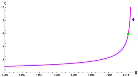
Figure 8. The variation of $g^{\prime }$ with g reveals that $g^{\prime }$ increases sharply toward infinity as g approaches 1.01467. Consequently, the self-consistent range in this case is restricted to a very narrow interval, $1<g<1.01467$. For reference, two points are marked in the figure: the blue point at ($g,g^{\prime }$) = (1.01489, 8.16425) represents the result obtained in Equation (59) of Section 3.1, while the green point at ($g,g^{\prime }$) = (1.01426, 5.93918) is obtained by substituting the predicted value $m_1=8.61\times {10}^{-3}$ eV from [34] into Equation (90). Notably, the blue point does not lie on the curve as in other cases $\mathbf{1},\mathbf{2}$, and 4; rather, it falls slightly to the right of the curve. This indicates that the test assumption employed in $\mathbf{Case}\mathbf{5}$ in Section 3.1 is inadequate. However, the region between these two points represents a key parameter space that future experimental designs should target for investigation.

Furthermore, Figure 9 presents the variation of $m_h$, $m_m$, and $m_l$ with respect to g. In this figure, when g approaches 1, we have $m_h\approx m_m\approx m_l$. However, as g increases beyond 1, $m_l$ begins to diverge from the other two. While $m_h$ and $m_m$ remain very close to each other, both soon approach approximately $5.01\times {10}^{-2}$ eV as g increases. In contrast, $m_l$ decreases rapidly to zero when g approaches 1.01467, at which point $g^2={\displaystyle \frac{{\Delta }_a}{{\Delta }_b}}$. Beyond this point, unphysical negative and imaginary neutrino masses appear.

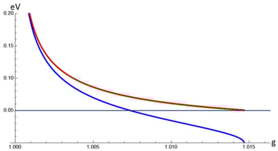
Figure 9. In this figure, the red, green, and blue curves represent the variations of $m_h$, $m_m$, and $m_l$ with respect to g, respectively. These variations reveal that the three neutrino masses are nearly degenerate when g is close to 1, with the red and green curves ($m_h$ and $m_m$) remaining almost overlapping throughout the entire physically allowed range. As g increases toward the critical value of 1.01467, $m_l$ (blue curve) separates from the other two and approaches zero. Beyond $g=1.01467$, the mass eigenvalues become unphysical, marking the boundary of the physically meaningful parameter space.

Consequently, physically reasonable neutrino masses satisfying $m_h>m_m>m_l>0$ arise only within a very narrow range $1<g<1.01467$. Two reference points are plotted in Figure 9: a blue point at $(g,g^{\prime })=(1.01489,8.16425)$, corresponding to the results obtained in Equation (59); and a green point at $(g,g^{\prime })=(1.01426,5.93918)$, obtained by substituting the previously predicted value $m_1=8.61\times {10}^{-3}$ eV into Equation (90). Unlike the previous cases, the blue point lies slightly to the right of the curve. At this point, Equation (59) yields an imaginary value for $m_l$, which indicates that the assumption ${\displaystyle \frac{m_h^2+m_m^2}{2}}\approx {\Delta }_a$ breaks down in this region. However, this discrepancy does not rule out the scenario; rather, it implies that the theoretically allowed upper bound of g is more tightly constrained. Therefore, the region of interest should be further restricted to the narrower interval $1.01426<g<1.01467$.

The preceding discussion has primarily focused on the region between the blue and green points in Figure 2, Figure 4, Figure 6, and Figure 8. However, there is no compelling reason to exclude the domain to the left of the green points, as it may conceal novel and intriguing possibilities. As shown in Figure 3, Figure 5, Figure 7, and Figure 9, when g approaches unity from the right, all three neutrino masses increase simultaneously. This behavior ensures consistency with the observed values of ${\Delta }_a$ and ${\Delta }_b$. This implies that even if individual neutrino masses are substantially large, the empirical MSDs, ${\Delta }_a$ and ${\Delta }_b$, can still remain small. Conversely, the observation of small MSDs does not preclude the possibility of neutrinos possessing very large individual masses, which would significantly enhance their overall contribution to the total mass of the Universe. This opens an especially promising avenue for future investigation.

Section Summary

The findings from all three subsections can be summarized as follows: This section explores various approaches to investigate neutrino masses. In Section 3.1, two of the six possible ways to match the two experimentally given values, ${\Delta }_a$ and ${\Delta }_b$, with the three theoretically defined MSDs ${\Delta }_{hm},{\Delta }_{ml}$, and ${\Delta }_{hl}$ are excluded due to inconsistencies. Among the remaining four viable cases, two exhibit $m_m\approx m_h$, while the other two exhibit $m_m\approx m_l$. Accordingly, we tested two approximations: (1) the midpoint approximation ${\Delta }_a\approx {\displaystyle \frac{m_h^2+m_m^2}{2}}$ for cases where $m_h\approx m_m$ (IO), and (2) ${\Delta }_b\approx {\displaystyle \frac{m_m^2+m_l^2}{2}}$ for cases where $m_m\approx m_l$ (NO).

As a result, $m_l$ is consistently predicted to be 6.09098 $\times {10}^{-3}$ eV in all cases, differing from previous analyses in [34]. The predictions for $m_h$ converge around $5.01\times {10}^{-2}$ eV in all cases. However, predictions for $m_m$ fall into two groups:

In $\mathbf{Cases}\mathbf{1}$ and $\mathbf{5}$, $m_m=4.97283\times {10}^{-2}$ eV is closer to $m_h$ (IO).

In $\mathbf{Cases}\mathbf{2}$ and $\mathbf{4}$, $m_m=1.05499\times {10}^{-2}$ eV is closer to $m_l$ (NO).

In Section 3.2, through analysis of the MSDs, all four viable cases predict an almost identical value for $\Delta m_{\left(\nu \right)}^2{=}_{4.5365}^{4.8129}\times {10}^{-64}$ GeV⁶, which is approximately 62 orders of magnitude smaller than the smallest $\Delta m_{\left(\mathcal{l}\right)}^2\approx 0.1107$ GeV⁶ of the charged leptons. With all four MSD products determined, the Jarlskog measure of CPV is also calculated, revealing that leptogenesis driven by Dirac neutrinos in the Standard Model and its minimal extension with sterile right-handed neutrinos is around 71 orders of magnitude smaller than baryogenesis in the current universe. This underscores the need for Beyond Standard Model (BSM) physics if we expect leptogenesis to play a significant role in resolving the Baryon Asymmetry of the Universe.

In Section 3.3, a more comprehensive analysis on the neutrino masses is provided. The self-consistent ranges of g and $g^{\prime }$ for each case are studied, and the variations of $g^{\prime }$, $m_h$, $m_m$, and $m_l$ with respect to g are plotted. The results can be summarized as follows:

1. Two Inverted ordering cases (1 and 5) suggest that $m_h\sim m_m\approx 5.01\times {10}^{-2}$ eV and $m_l\approx 6.09098\times {10}^{-3}$ eV, with g constrained to very narrow ranges:

$$\begin{array}{ccc}\hfill 1& <& g<1.01512\mathrm{in}\mathbf{Case}\mathbf{1},\hfill \end{array}$$

(91)

$$\begin{array}{ccc}\hfill 1& <& g<1.01467\mathrm{in}\mathbf{Case}\mathbf{5}.\hfill \end{array}$$

(92)

2. The other two Normal ordering cases (2 and 4) indicate wider ranges:

$$\begin{array}{ccc}\hfill 1& <& g<5.81614\mathrm{in}\mathbf{Case}\mathbf{2},\hfill \end{array}$$

(93)

$$\begin{array}{ccc}\hfill 1& <& g<5.90148\mathrm{in}\mathbf{Case}\mathbf{4}.\hfill \end{array}$$

(94)

In addition, two reference points are plotted in Figure 2, Figure 4, Figure 6 and Figure 8, respectively, to illustrate the results previously analyzed. The intervals between each pair of points highlight the significant ranges of the variable g in the corresponding cases:

$$\begin{array}{ccc}\hfill 1.01467& <& g<1.01489\mathrm{in}\mathbf{Case}\mathbf{1},\hfill \end{array}$$

(95)

$$\begin{array}{ccc}\hfill 4.17388& <& g<4.78383\mathrm{in}\mathbf{Case}\mathbf{2},\hfill \end{array}$$

(96)

$$\begin{array}{ccc}\hfill 4.23338& <& g<4.85301\mathrm{in}\mathbf{Case}\mathbf{4},\hfill \end{array}$$

(97)

$$\begin{array}{ccc}\hfill 1.01426& <& g<1.01467\mathrm{in}\mathbf{Case}\mathbf{5}.\hfill \end{array}$$

(98)

These ranges correspond to the following intervals of the lightest neutrino mass $m_l$:

$$\begin{array}{ccc}\hfill 8.64611\times {10}^{-3}\mathrm{eV}& >& m_l>6.11487\times {10}^{-3}\mathrm{eV},\hfill \end{array}$$

(99)

$$\begin{array}{ccc}\hfill 8.60999\times {10}^{-3}\mathrm{eV}& >& m_l>6.09096\times {10}^{-3}\mathrm{eV},\hfill \end{array}$$

(100)

$$\begin{array}{ccc}\hfill 8.60999\times {10}^{-3}\mathrm{eV}& >& m_l>6.09096\times {10}^{-3}\mathrm{eV},\hfill \end{array}$$

(101)

$$\begin{array}{ccc}\hfill 8.55943\times {10}^{-3}\mathrm{eV}& >& m_l>7.45159\times {10}^{-4}\mathrm{eV},\hfill \end{array}$$

(102)

respectively. These intervals represent parameter regions that warrant closer attention in future analyses. Notably, the lower bound $7.45159\times {10}^{-4}$ eV of $m_l$ in Equation (102) (Case 5) extends to a value significantly lower than those in the other three cases.

4. Conclusions and Discussion

In conclusion, this article has analyzed the neutrino mass spectrum within an analytically solvable CP-Violating Standard Model (CPVSM). By employing two experimentally measured mass squared differences (MSDs) alongside the fundamental relationship ${\Delta }_{hm}+{\Delta }_{ml}\equiv {\Delta }_{hl}$ defined in Equation (2), we have successfully determined the third MSD across various scenarios. This methodology enables calculation of the MSD product in the neutrino sector, $\Delta m_{\left(\nu \right)}^2\equiv {({\Delta }_{hm}·{\Delta }_{ml}·{\Delta }_{hl})}_{\left(\nu \right)}$ as defined in Equation (71), facilitating an estimation of leptogenesis magnitude and its comparison with baryogenesis.

In Section 3.1, we examined six potential correspondences between two experimentally determined MSDs, ${\Delta }_a$ and ${\Delta }_b$, and the three theoretically defined quantities ${\Delta }_{hm}$, ${\Delta }_{ml}$, and ${\Delta }_{hl}$. Two correspondences were ruled out due to inconsistencies, leaving four viable cases for detailed investigation.

Section 3.2 presented a comprehensive analysis of MSDs across all four viable cases. With all twelve MSDs determined for the four fermion types, we evaluated leptogenesis in the lepton sector and baryogenesis in the quark sector. By incorporating these results into the Jarlskog measure of CP violation along with the current experimental estimate of the leptonic Jarlskog invariant $J_{\left(l\right)}$, we found that leptogenesis is at least 71 orders of magnitude weaker than baryogenesis within this CPVSM framework. This striking disparity reveals a critical need for physics Beyond the Standard Model if leptogenesis is expected to contribute significantly to the observed Baryon Asymmetry of the Universe.

Section 3.3 derived analytical expressions describing how the masses $m_h$, $m_m$, $m_l$, and the ratio $g^{\prime }\equiv {\displaystyle \frac{m_m}{m_l}}$ vary as functions of the mass ratio $g\equiv {\displaystyle \frac{m_h}{m_m}}$. The four cases divide into two classes with distinct predictions. Class 1 ($\mathbf{Cases}\mathbf{1}$ and $\mathbf{5}$) yields narrow ranges, $1<g<1.01512$ and $1<g<1.01467$ respectively, suggesting $m_m$ is closer to $m_h$ (IO). Class 2 ($\mathbf{Cases}\mathbf{2}$ and $\mathbf{4}$) allows broader ranges, $1<g<5.81614$ and $1<g<5.90148$ respectively, suggesting $m_m$ is closer to $m_l$ (NO).

All four cases predict similar values for the heaviest neutrino mass, $m_h\approx 5.01\times {10}^{-2}$ eV, and the lightest neutrino mass, $m_l\approx 6.09098\times {10}^{-3}$ eV. For the middle neutrino mass, the model offers two possibilities: either $m_m\approx 4.973\times {10}^{-2}$ eV if $m_m$ is closer to $m_h$ (Class 1, IO), or $m_m\approx 1.015\times {10}^{-2}$ eV if $m_m$ is closer to $m_l$ (Class 2, NO). The predicted lightest mass differs slightly from the value $m_1=8.61\times {10}^{-3}$ eV reported in [34], which corresponds to the square root of ${\Delta }_b$. Each case contains a distinct region of interest between the blue and green points shown in Figure 2, Figure 4, Figure 6, and Figure 8.

Regarding mass degeneracy, we found that as $\mathbf{C}$ approaches zero, two eigenvalues become degenerate, while all three eigenvalues become degenerate when both $\mathbf{B}$ and $\mathbf{C}$ (equivalently, $\beta$ and $\gamma$) approach zero and g tends to unity. This indicates that CP symmetry violation is intrinsically linked to the breaking of $S_N$ symmetry, though not necessarily to mass degeneracy itself. The mechanism by which $\mathbf{C}$ acquires its non-trivial value remains under investigation and may be related to the universe’s cooling during expansion. Combining the discussions regarding mass degeneracy and MSDs, the eigenvalue patterns obtained in such a framework hint at the possibility that absolute neutrino masses could be very large even the MSDs remain small.

These theoretical predictions are expected to be testable in the near future through ongoing and planned neutrino experiments, offering valuable insights into neutrino mass hierarchies and CP violation in the lepton sector.

References

- Christenson, J.H.; Cronin, J.; Fitch, V.L.; Turlay, R. Evidence for the 2 π Decay of the Meson. Phys. Rev. Lett. 1964, 13, 138. [Google Scholar] [CrossRef]
- Lin, C.L. An Improved Standard Model Comes with Explicit CPV and Productive of BAU. J. Mod. Phys. 2020, 11, 1157–1169. [Google Scholar] [CrossRef]
- Lin, C.L. Exploring the Origin of CP Violation in the Standard Model. Lett. High Energy Phys. 2021, 221, 1. [Google Scholar] [CrossRef]
- Lin, C.L. BAU Production in the SN-Breaking Standard Model. Symmetry 2023, 15, 1051. [Google Scholar] [CrossRef]
- Cabibbo, N. Unitary symmetry and leptonic decays. Phys. Rev. Lett. 1963, 10, 531. [Google Scholar] [CrossRef]
- Kobayashi, M.; Maskawa, T. CP-violation in the renormalizable theory of weak interaction. Prog. Theor. Phys. 1973, 49, 652–657. [Google Scholar] [CrossRef]
- Davis, R., Jr.; Harmer, D.S.; Hoffman, K.C. Search for neutrinos from the sun. Phys. Rev. Lett. 1968, 20, 1205. [Google Scholar] [CrossRef]
- Davis, R., Jr. A review of the Homestake solar neutrino experiment. Prog. Part. Nucl. Phys. 1994, 32, 13–32. [Google Scholar] [CrossRef]
- Abdurashitov, J.N.; Gavrin, V.N.; Gorbachev, V.V.; Gurkina, P.P.; Ibragimova, T.V.; Kalikhov, A.V.; Khairnasov, N.G.; Knodel, T.V.; Mirmov, I.N.; SAGE Collaboration; et al. Measurement of the solar neutrino capture rate with gallium metal. III. Results for the 2002–2007 data-taking period. Phys. Rev. C 2009, 80, 015807. [Google Scholar] [CrossRef]
- Hampel, W.; Handt, J.; Heusser, G.; Kiko, J.; Kirsten, T.; Laubenstein, M.; Pernicka, E.; Rau, W.; Wojcik, M.; Zakharov, Y.; et al. GALLEX solar neutrino observations: Results for GALLEX IV. Phys. Lett. B 1999, 447, 127–133. [Google Scholar] [CrossRef]
- Altmann, M.; Balata, M.; Belli, P.; Bellotti, E.; Bernabei, R.; Burkert, E.; Cattadori, C.; Cerulli, R.; Chiarini, M.; Cribier, M.; et al. Complete results for five years of GNO solar neutrino observations. Phys. Lett. B 2005, 616, 174. [Google Scholar] [CrossRef]
- Ahmad, Q.R.; Allen, R.C.; Andersen, T.C.; Anglin, J.D.; Bühler, G.; Barton, J.C.; Beier, E.W.; Bercovitch, M.; Bigu, J.; Biller, S.; et al. Measurement of the Rate of ve + d → p + p + e− Interactions Produced by 8B Solar Neutrinos at the Sudbury Neutrino Observatory. Phys. Rev. Lett. 2001, 87, 071301. [Google Scholar] [CrossRef] [PubMed]
- Ahmad, Q.R.; Allen, R.C.; Andersen, T.C.; Anglin, J.D.; Barton, J.C.; Beier, E.W.; Bercovitch, M.; Bigu, J.; Biller, S.D.; Black, R.A.; et al. Direct evidence for neutrino flavor transformation from neutral-current interactions in the Sudbury Neutrino Observatory. Phys. Rev. Lett. 2002, 89, 011301. [Google Scholar] [CrossRef] [PubMed]
- Hirata, K.S.; Kajita, T.; Koshiba, M.; Nakahata, M.; Ohara, S.; Oyama, Y.; Sato, N.; Suzuki, A.; Takita, M.; Totsuka, Y.; et al. Experimental study of the atmospheric neutrino flux. Phys. Lett. B 1988, 205, 416–420. [Google Scholar] [CrossRef]
- Hirata, K.S.; Inoue, K.; Ishida, T.; Kajita, T.; Kihara, K.; Nakahata, M.; Ohara, S.; Sakai, A.; Sato, N.; Suzuki, Y.; et al. Observation of a small atmospheric νμ/νe ratio in Kamiokande. Phys. Lett. B 1992, 280, 146–152. [Google Scholar] [CrossRef]
- Fukuda, Y.; Hayakawa, T.; Ichihara, E.; Inoue, K.; Ishihara, K.; Ishino, H.; Itow, Y.; Kajita, T.; Kameda, J.; Kasuga, S.; et al. Evidence for oscillation of atmospheric neutrinos. Phys. Rev. Lett. 1998, 81, 1562. [Google Scholar] [CrossRef]
- Fukuda, S.; Fukuda, Y.; Ishitsuka, M.; Itow, Y.; Kajita, T.; Kameda, J.; Kaneyuki, K.; Kobayashi, K.; Koshio, Y.; Miura, M.; et al. Tau neutrinos favored over sterile neutrinos in atmospheric muon neutrino oscillations. Phys. Rev. Lett. 2000, 85, 3999. [Google Scholar] [CrossRef]
- Eguchi, K.; Enomoto, S.; Furuno, K.; Goldman, J.; Hanada, H.; Ikeda, H.; Ikeda, K.; Inoue, K.; Ishihara, K.; Itoh, W.; et al. First results from KamLAND: Evidence for reactor antineutrino disappearance. Phys. Rev. Lett. 2003, 90, 021802. [Google Scholar] [CrossRef]
- Araki, T.; Eguchi, K.; Enomoto, S.; Furuno, K.; Ichimura, K.; Ikeda, H.; Inoue, K.; Ishihara, K.; Iwamoto, T.; Kawashima, T.; et al. Measurement of neutrino oscillation with KamLAND: Evidence of spectral distortion. Phys. Rev. Lett. 2005, 94, 081801. [Google Scholar] [CrossRef]
- An, F.P.; Bai, J.Z.; Balantekin, A.B.; Band, H.R.; Beavis, D.; Beriguete, W.; Bishai, M.; Blyth, S.; Boddy, K.; Brown, R.L.; et al. Observation of electron-antineutrino disappearance at Daya Bay. Phys. Rev. Lett. 2012, 108, 171803. [Google Scholar] [CrossRef]
- An, F.P.; Balantekin, A.B.; Band, H.R.; Bishai, M.; Blyth, S.; Cao, D.; Cao, G.F.; Cao, J.; Cen, W.R.; Chan, Y.L.; et al. Measurement of electron antineutrino oscillation based on 1230 days of operation of the Daya Bay experiment. Phys. Rev. D 2017, 95, 072006. [Google Scholar] [CrossRef]
- Ahn, J.K.; Chebotaryov, S.; Choi, J.H.; Choi, S.; Choi, W.; Choi, Y.; Jang, H.I.; Jang, J.S.; Jeon, E.J.; Jeong, I.S.; et al. Observation of reactor electron antineutrinos disappearance in the RENO experiment. Phys. Rev. Lett. 2012, 108, 191802. [Google Scholar] [CrossRef]
- Abe, Y.; Aberle, C.; Akiri, T.; dos Anjos, J.C.; Ardellier, F.; Barbosa, A.F.; Baxter, A.; Bergevin, M.; Bernstein, A.; Bezerra, T.J.C.; et al. Indication of Reactor Disappearance in the Double Chooz Experiment. Phys. Rev. Lett. 2012, 108, 131801. [Google Scholar] [CrossRef] [PubMed]
- Ahn, M.H.; Aliu, E.; Andringa, S.; Aoki, S.; Aoyama, Y.; Argyriades, J.; Asakura, K.; Ashie, R.; Berghaus, F.; Berns, H.G.; et al. Measurement of neutrino oscillation by the K2K experiment. Phys. Rev. D 2006, 74, 072003. [Google Scholar] [CrossRef]
- Michael, D.G.; Adamson, P.; Alexopoulos, T.; Allison, W.W.M.; Alner, G.J.; Anderson, K.; Andreopoulos, C.; Andrews, M.; Andrews, R.; Arms, K.E.; et al. Observation of Muon Neutrino Disappearance with the MINOS Detectors in the NuMI Neutrino Beam. Phys. Rev. Lett. 2006, 97, 191801. [Google Scholar] [CrossRef] [PubMed]
- Adamson, P.; Andreopoulos, C.; Arms, K.E.; Armstrong, R.; Auty, D.J.; Ayres, D.S.; Baller, B.; Barnes, P.D., Jr.; Barr, G.; Barrett, W.L.; et al. Measurement of neutrino oscillations with the MINOS detectors in the NuMI beam. Phys. Rev. Lett. 2008, 101, 131802. [Google Scholar] [CrossRef]
- Abe, K.; Abgrall, N.; Ajima, Y.; Aihara, H.; Albert, J.B.; Andreopoulos, C.; Andrieu, B.; Aoki, S.; Araoka, O.; Argyriades, J.; et al. Indication of Electron Neutrino Appearance from an Accelerator-Produced Off-Axis Muon Neutrino Beam. Phys. Rev. Lett. 2011, 107, 041801. [Google Scholar] [CrossRef]
- Abe, K.; Amey, J.; Andreopoulos, C.; Antonova, M.; Aoki, S.; Ariga, A.; Ashida, Y.; Ban, S.; Barbi, M.; Barker, G.J.; et al. Measurement of neutrino and antineutrino oscillations by the T2K experiment including a new additional sample of ve interactions at the far detector. Phys. Rev. D 2017, 96, 092006. [Google Scholar] [CrossRef]
- Adamson, P.; Ader, C.; Andrews, M.; Anfimov, N.; Anghel, I.; Arms, K.; Arrieta-Diaz, E.; Aurisano, A.; Ayres, D.S.; Backhouse, C.; et al. First measurement of electron neutrino appearance in NOvA. Phys. Rev. Lett. 2016, 116, 151806. [Google Scholar] [CrossRef]
- Adamson, P.; Aliaga, L.; Ambrose, D.; Anfimov, N.; Antoshkin, A.; Arrieta-Diaz, E.; Augsten, K.; Aurisano, A.; Backhouse, C.; Baird, M.; et al. Search for active-sterile neutrino mixing using neutral-current interactions in NOvA. Phys. Rev. D 2017, 96, 072006. [Google Scholar] [CrossRef]
- Gonzalez-Garcia, M.C.; Maltoni, M.; Schwetz, T. Updated fit to three neutrino mixing: Status of leptonic CP violation. JHEP 2014, 11, 052. [Google Scholar] [CrossRef]
- Ambrosio, M.; Antolini, R.; Auriemma, G.; Bakari, D.; Baldini, A.; Barbarino, G.C.; Barish, B.C.; Battistoni, G.; Becherini, Y.; Bellotti, R.; et al. Matter effects in upward-going muons and sterile neutrino oscillations. Phys. Lett. B 2001, 517, 59. [Google Scholar] [CrossRef]
- Sanchez, M.; Allison, W.W.M.; Alner, G.J.; Ayres, D.S.; Barrett, W.L.; Border, P.M.; Cobb, J.H.; Cockerill, D.J.A.; Courant, H.; Demuth, D.M.; et al. Measurement of the L/E distributions of atmospheric ν in Soudan 2 and their interpretation as neutrino oscillations. Phys. Rev. D 2003, 68, 113004. [Google Scholar] [CrossRef]
- Esteban, I.; Gonzalez-Garcia, M.C.; Maltoni, M.; Schwetz, T.; Zhou, T. The fate of hints: Updated global analysis of three-flavor neutrino oscillations. JHEP 2020, 9, 178. [Google Scholar] [CrossRef]
- Jarlskog, C. Commutator of the quark mass matrices in the standard electroweak model and a measure of maximal CP nonconservation. Phys. Rev. Lett. 1985, 55, 1039. [Google Scholar] [CrossRef] [PubMed]
- Pontecorvo, B. Mesonium and antimesonium. Sov. Phys. JETP 1957, 6, 429. [Google Scholar]
- Pontecorvo, B. Neutrino experiments and the problem of conservation of leptonic charge. Sov. Phys. JETP 1968, 26, 165. [Google Scholar]
- Maki, Z.; Nakagawa, M.; Sakata, S. Remarks on the unified model of elementary particles. Prog. Theor. Phys. 1962, 28, 870–880. [Google Scholar] [CrossRef]
- Shaposhnikov, M.E. Baryon asymmetry of the universe in standard electroweak theory. Nucl. Phys. B 1987, 287, 757–775. [Google Scholar] [CrossRef]
- D’Onofrio, M.; Ummukainen, K. Standard model cross-over on the lattice. Phys. Rev. D 2016, 93, 025003. [Google Scholar] [CrossRef]
- Lin, C.L.; Lee, C.E.; Yang, Y.W. The Two Higgs-Doublet Extension of the Standard Model and S3 Symmetry. Chin. J. Phys. 1988, 26, 180. [Google Scholar]
- Almumin, Y.; Chen, M.C.; Cheng, M.; Knapp-Perez, V.; Li, Y.; Mondol, A.; Ramos-Sanchez, S.; Ratz, M.; Shukla, S. Neutrino Flavor Model Building and the Origins of Flavor and CP Violation: A Snowmass White Paper. arXiv 2022, arXiv:2204.08668. [Google Scholar] [CrossRef]
- Zyla, P.A.; Barnett, R.M.; Beringer, J.; Dahl, O.; Dwyer, D.A.; Groom, D.E.; Lin, C.-J.; Lugovsky, K.S.; Pianori, E.; Robinson, D.J.; et al. Review of Particle Physics. Prog. Theor. Exp. Phys. 2020, 2020, 083C01. [Google Scholar] [CrossRef]
Disclaimer/Publisher’s Note: The statements, opinions and data contained in all publications are solely those of the individual author(s) and contributor(s) and not of MDPI and/or the editor(s). MDPI and/or the editor(s) disclaim responsibility for any injury to people or property resulting from any ideas, methods, instructions or products referred to in the content. |
© 2025 by the author. Licensee MDPI, Basel, Switzerland. This article is an open access article distributed under the terms and conditions of the Creative Commons Attribution (CC BY) license (https://creativecommons.org/licenses/by/4.0/).