DdONN-PINNs: Complex Optical Wavefield Reconstruction by Domain Decomposition of Optical Neural Networks and Physics-Informed Information

Abstract

To address the challenges of poor adaptability to spatial heterogeneity, easy breakage of amplitude–phase coupling relationships, and insufficient physical consistency in complex optical wavefield reconstruction, this paper proposes the DdONN-PINNs hybrid framework. Focused on preserving the intrinsic symmetries of wave physics, the framework achieves deep integration of optical neural networks and physics-informed information. Centered on an architecture of “SIREN shared encoding–domain-specific output”, it utilizes the periodic activation property of SIREN encoders to maintain the spatial symmetry of wavefield distribution, incorporates learnable Fourier diffraction layers to model physical propagation processes, and adopts native complex-domain modeling to avoid splitting the real and imaginary parts of complex amplitudes—effectively adapting to spatial heterogeneity while fully preserving amplitude-phase coupling in wavefields. Validated on rogue wavefields governed by the Nonlinear Schrödinger Equation (NLSE), experimental results demonstrate that DdONN-PINNs achieve an amplitude Mean Squared Error (MSE) of $2.94\times {10}^{-3}$ and a phase MSE of $5.86\times {10}^{-4}$, outperforming non-domain-decomposed models and ReLU-activated variants significantly. Robustness analysis shows stable reconstruction performance even at a noise level of $\sigma =0.1$. This framework provides a balanced solution for wavefield reconstruction that integrates precision, physical interpretability, and robustness, with potential applications in fiber-optic communication and ocean optics.

1. Introduction

Optical Neural Networks (ONNs), as a novel computational paradigm integrating optical propagation mechanisms with deep learning frameworks, exhibit unique advantages in tasks such as image recognition, wavefield reconstruction, and optical inversion, utilizing the inherent parallelism, low energy consumption, and complex-domain modeling capabilities of photons [1,2]. Unlike traditional electronic neural networks, ONNs utilize light’s amplitude, phase, and polarization as information carriers, performing computations through optical processes like diffraction and interference rather than relying on voltage and current. This physical mechanism enables them to directly adapt to parallel processing of two-dimensional wavefield data. For instance, real-time Fourier transforms can be achieved via 4f systems, leading to an order-of-magnitude acceleration in inference speed compared to electronic chips [3,4]. In some experiments on photonics-based ONNs, energy efficiency has been improved by up to three orders of magnitude compared to traditional GPUs, providing a new pathway for energy-efficient physical field modeling [5,6].

Despite ONNs’ advantages in parallelism and low energy consumption, their inherent limitations have been highlighted in modern reviews [7,8]. Ma et al. [7] noted ONNs’ energy efficiency is bounded by noise. Kazanskiy et al. [8] further summarized core ONN bottlenecks: difficulty in effective optical nonlinearity, high noise sensitivity, and poor integration with electronic systems. Though hybrid electro-optic platforms or meta-materials are explored as solutions, they often increase complexity or reduce compactness.

In recent years, the development of ONNs has shown a trend of collaborative innovation between algorithms and hardware. At the algorithmic level, Lin et al. pioneered the Diffractive Deep Neural Networks (D2NNs), realizing all-optical information processing through deep learning-designed multi-layer diffractive layers, which provided a purely optical solution for tasks such as image classification and laid the foundation for modern diffractive optical networks [9]. Building on this, Rahman et al. further improved the robustness and generalization ability of networks by integrating multiple diffractive optical subnetwork models [10]. Jagtap et al. proposed Extended Physics-Informed Neural Networks (XPINNs), which verified the effectiveness of allocating model capacity according to regional characteristics for complex system modeling through generalized spatiotemporal domain decomposition, providing theoretical support for the domain decomposition strategy [11]. In terms of hardware, Zhong et al. designed a graphene/silicon heterojunction structure to achieve reconfigurable phase response functions, breaking the fixed limitation of traditional optical activation functions [12]. Gu et al. proposed the planar diffractive neural network (pla-NN), which solved the alignment deviation problem of diffractive systems based on printed circuit technology, promoting the integration and practical application of ONNs [13]. These advancements have collectively driven ONNs to evolve from static architectures to end-to-end trainable intelligent systems.

Meanwhile, the rise of Physics-Informed Neural Networks (PINNs) has injected physical interpretability into neural networks. The PINNs framework proposed by Raissi et al. realizes collaborative modeling of data-driven and physical constraints by embedding partial differential equation residuals into the loss function [14]. Subsequent studies have further developed mechanisms such as multi-level domain decomposition (Dolea et al.) and gradient enhancement (Barbulescu et al.) to improve modeling accuracy for strongly nonlinear systems [15,16]. Chong et al.’s Physics-Guided Neural Network (PGNN) verified the principle that physical constraints enhance model robustness in the estimation of tissue optical properties, providing practical references for physics–data fusion in the optical field [17].

Existing diffractive ONNs and PINNs encounter certain structural challenges when addressing complex wavefield reconstruction tasks. Specifically, diffractive ONNs typically employ a global diffractive layer for unified modeling, which may not fully account for the spatial heterogeneity of wavefields, such as the high-frequency characteristics in core regions and the low-frequency characteristics in edge regions. This approach could potentially lead to the loss of high-frequency details and overfitting in low-frequency areas. Meanwhile, PINNs apply uniform physical constraints across the entire field through a single residual loss, which may be less effective in strongly nonlinear regions and could result in over-penalization in flat regions. These observations suggest that there may be room for further optimization in existing methods to better accommodate the characteristics of different regions. More critically, existing methods generally split complex amplitudes into real and imaginary parts for independent processing, severing the intrinsic coupling between amplitude and phase. This fails to meet the structure-preserving requirements of wave equations and neglects the advantages of the complex domain in higher expressive capacity and noise-robust memory [18].

Notably, even advanced complex-valued PINN variants face this trade-off: Sinusoidal Representation Network (SIREN)-based complex models [19] uses periodic activations to inherently retain amplitude-phase coupling and ensure high-order derivative continuity—key for NLSE wavefields—but their unified network architecture lacks adaptability to spatial heterogeneity, failing to prioritize nonlinear dynamics in high-gradient core regions. Conversely, complex-valued PINNs (CV-PINNs) with domain-adapted sampling [20] improve spatial fitting for heterogeneous wavefields, yet their real–imaginary split representations (adopted for optimization simplicity) disrupt amplitude-phase integrity, leading to phase mean squared error over $2\times$ higher than native complex SIRENs and violating NLSE analyticity.

To address these issues, this paper proposes a hybrid framework of DdONN-PINNs:; it precisely characterizes spatial through a domain decomposition strategy, embeds physical propagation processes via learnable Fourier diffraction layers, realizes data–physics dual-driven optimization using adaptive sampling [21] and gradient enhancement mechanisms [22], and completely preserves amplitude-phase coupling through native complex-domain modeling, thereby achieving the unification of numerical accuracy and physical conservation within the same framework.

The structure of this paper is as follows:. Section 2 details the architectural design of DdONN-PINNs, including the domain decomposition strategy, physical embedding mechanism, loss function, and training optimization. Section 3 presents the key modules of the algorithm in the form of pseudocode. Section 4 verifies the accuracy, physical consistency, and noise resistance of the method based on the reconstruction task of nonlinear Schrödinger equation (NLSE) rogue wavefields, and compares the numerical results with those of the non-domain-decomposed ONN-PINNs and DdONN-PINNs with ReLU activation function. Section 5 summarizes the research findings and prospects its application in fields such as optical fiber communication and ocean optics.

In what follows, the following notations are used throughout the paper. $\mathbf{x}$ denotes the 2D spatial coordinate vector of the optical wavefield ($\mathbf{x}=(x,y)$), with x and y representing horizontal and vertical coordinates in the optical propagation plane; t represents the time variable, describing the temporal evolution of the complex optical wavefield. $u(\mathbf{x},t)$ is the true complex optical wavefield, expressed as $u(\mathbf{x},t)=A(\mathbf{x},t)e^{i\varphi (\mathbf{x},t)}$—where $A(\mathbf{x},t)$ is the non-negative amplitude and $\varphi (\mathbf{x},t)$ is the phase (real value in $[-\pi ,\pi ]$). $u^{\mathrm{obs}}(\mathbf{x},t)$ denotes noisy observed data (Gaussian noise added to $u(\mathbf{x},t)$, consistent with optical measurements); $\widehat{u}(\mathbf{x},t)$ is the DdONN-PINNs-predicted wavefield, with amplitude $\widehat{A}(\mathbf{x},t)=\left|\widehat{u}(\mathbf{x},t)\right|$ and phase $\widehat{\varphi }(\mathbf{x},t)=arg\left(\widehat{u}(\mathbf{x},t)\right)$. $\mathcal{N}[·]$ is the physical residual operator, quantifying $\widehat{u}$’s deviation from fundamental optical laws (e.g., diffraction, energy conservation); $\mathbb{E}[·]$ is the spatial expectation operator (spatial average) for global wavefield properties; ${\parallel ·\parallel }^2$ is the squared $L_2$ norm, quantifying discrepancies between wavefields. ${\mathcal{L}}_{\mathrm{data}}={\parallel \widehat{u}-u^{\mathrm{obs}}\parallel }^2$ is the data fitting loss, minimizing prediction–observation gaps. ${\mathcal{L}}_{\mathrm{constraint}}={\mathcal{L}}_{\mathrm{phys}}+{\mathcal{L}}_{\mathrm{grad}}+{\mathcal{L}}_{\mathrm{scale}}+{\mathcal{L}}_{\mathrm{smooth}}$ is the physical constraint set: ${\mathcal{L}}_{\mathrm{phys}}={\parallel \mathcal{N}\left[\widehat{u}\right]\parallel }^2$ enforces optical law compliance; ${\mathcal{L}}_{\mathrm{grad}}={\parallel \nabla \mathcal{N}\left[\widehat{u}\right]\parallel }^2$ enhances residual smoothness; ${\mathcal{L}}_{\mathrm{scale}}=|{\overline{A}}_{\mathrm{pred}}-{\overline{A}}_{\mathrm{true}}|$ maintains energy scale (${\overline{A}}_{\mathrm{pred}}=\mathbb{E}\left[\right|\widehat{u}\left|\right]$, ${\overline{A}}_{\mathrm{true}}=\mathbb{E}\left[\right|u^{\mathrm{obs}}\left|\right]$); ${\mathcal{L}}_{\mathrm{smooth}}=\mathbb{E}\left[\right|\nabla \widehat{\varphi }\left|\right]$ suppresses phase discontinuities. ${\mathcal{L}}_{\mathrm{total}}={\mathcal{L}}_{\mathrm{data}}+\alpha \left(t\right){\mathcal{L}}_{\mathrm{constraint}}$ is the total training loss, where $\alpha \left(t\right)$ is a dynamic weight balancing data fitting and physical consistency.

2. DdONN-PINNs

To clearly elaborate on the design philosophy and working mechanism of DdONN-PINNs, this section starts from the overall architecture, first intuitively presenting its core framework and closed-loop process through a block diagram, and then delving into the composition principles of each key module layer by layer.

2.1. DdONN-PINNs Framework

Figure 1 shows the hybrid training framework integrating DdONN and PINNs, clearly depicting the complete closed-loop process from physical input to model optimization. Through the synergistic constraints of physical information and data-driven mechanisms, this framework achieves high-precision modeling of complex wavefields $\widehat{u}(\mathbf{x},t)$.

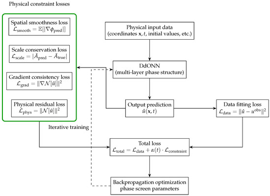
Figure 1. DdONN-PINNs training closed-loop: Physical input generates the wavefield $\widehat{u}(\mathbf{x},t)$ through the complex-domain DdONN. The total loss ${\mathcal{L}}_{\mathrm{total}}$ integrates two parts: (1) the data fitting loss ${\mathcal{L}}_{\mathrm{data}}$ to match observations, and (2) a set of physical constraint losses, ${\mathcal{L}}_{\mathrm{constraint}}$ including ${\mathcal{L}}_{\mathrm{phys}}$, ${\mathcal{L}}_{\mathrm{grad}}$, ${\mathcal{L}}_{\mathrm{scale}}$, ${\mathcal{L}}_{\mathrm{smooth}}$, weighted by $\alpha \left(t\right)$.

Forward propagation starts with physical input data (including spatial coordinates $\mathbf{x}$, time t, and initial conditions). The input is fed into DdONN, where feature mapping and nonlinear transformation are performed through multi-layer phase modulation, ultimately outputting the wavefield prediction result $\widehat{u}(\mathbf{x},t)$. The loss function adopts a dual-constraint mechanism, including the physical residual loss ${\mathcal{L}}_{\mathrm{phys}}={\parallel \mathcal{N}\left[\widehat{u}\right]\parallel }^2$ and the data fitting loss ${\mathcal{L}}_{\mathrm{data}}={\parallel \widehat{u}-u^{\mathrm{obs}}\parallel }^2$. These two losses are aggregated to form the total loss ${\mathcal{L}}_{\mathrm{total}}={\mathcal{L}}_{\mathrm{data}}+\alpha \left(t\right)·{\mathcal{L}}_{\mathrm{constraint}}$, ensuring that the model output satisfies both physical laws and observed data. The optimization process optimizes the core parameters of DdONN (phase screen parameters) through backpropagation, forming an iterative training closed-loop of prediction–loss calculation–parameter update until the model converges to a stable state.

The core innovation of this framework lies in the deep integration of optical neural networks and physical constraints. The multi-layer phase structure of DdONN is naturally adapted to the spatial modulation characteristics of wavefields, while the dual loss functions constrain the prediction results from the two dimensions of physical rationality and data consistency. Finally, through iterative optimization, the unification of high precision–physical self-consistency in wavefield modeling is achieved, providing a solution with both physical interpretability and modeling flexibility for numerical simulation of complex nonlinear wavefields.

Next, we will introduce the architecture of each module in DdONN-PINNs one by one, including DdONN, SIREN [19] encoding network, domain-specific output heads, domain fusion and complex assembly, multi-layer learnable diffraction propagation, and loss function design.

2.2. DdONN Architecture

Figure 2 presents the general structural framework of DdONN, clearly embodying the progressive design concept of encoding–domain decomposition–complex field assembly–diffraction.

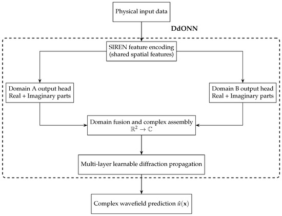
Figure 2. DdONN pipeline: SIREN encoding → regional heads → complex fusion → learnable diffraction, yielding $\widehat{u}(\mathbf{x},t)$.

DdONN concatenates a shared SIREN encoder with region-specific decoders. Coordinates $(\mathbf{x},t)$ are first mapped to a continuous latent space $\mathbf{f}(\mathbf{x},t)$ by SIREN; two parallel heads then generate real and imaginary components for Domain A and Domain B, respectively. These components are fused into a single complex amplitude field and propagated through learnable diffractive layers to obtain $\widehat{u}(\mathbf{x},t)$. This hierarchy—shared features, regional specialization, complex recombination, and physics-aware propagation—delivers accurate, interpretable wavefield reconstructions across scales.

2.3. SIREN Encoding Network

Figure 3 illustrates the scalable hierarchical architecture of the SIREN feature encoding module, intuitively presenting its structural design and flexibility.

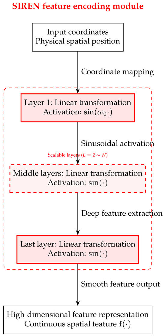
Figure 3. SIREN encoding: fixed $sin({\omega }_0·)$ layer for low-frequency anchoring, scalable $sin(·)$ layers for high-frequency detail, yielding continuous spatial features.

SIREN serves as the shared encoder of DdONN. Input coordinates $(\mathbf{x},t)$ are first mapped by a fixed initial layer with modulation frequency ${\omega }_0$ to establish the low-frequency backbone. A cascade of $N-2$ intermediate layers—each parameterized by learnable linear transforms followed by sinusoidal activations—progressively refines the representation to encode high-order spatial correlations. The final fixed layer aggregates these intermediate features into a continuous, differentiable, high-dimensional embedding $\mathbf{f}(\mathbf{x},t)\in {\mathbb{R}}^D$ that retains global smoothness while capturing fine-scale structures. This architecture circumvents the spectral bias of piece-wise linear activations and supplies domain-specific decoders with physically consistent features for subsequent wavefield reconstruction.

SIREN employs $sin(·)$ activations to construct an infinitely differentiable, globally smooth latent space $\mathbf{f}(\mathbf{x},t)$ from $(\mathbf{x},t)$, eliminating spectral bias and enabling region-specific decoders to produce physically-consistent wavefield estimates.

2.4. Domain-Specific Output Heads

Figure 4 illustrates the general architecture of domain-specific output heads and their mechanism for region-differentiated modeling of complex optical wavefields. For this modeling, the domain decomposition relies on a predefined fixed spatial mask—its design rooted in experimental observations of complex optical wave behaviors; in practical optical systems (e.g., laser propagation, holographic imaging), optical wavefields (including optical rogue waves) concentrate most energy (light intensity) and interference gradients (fringe density) in a central region, while the surrounding edge area exhibits smooth dynamics dominated by diffraction effects. This mask is fixed once determined and not adjusted epoch-wise, ensuring alignment with real optical physics and avoiding training instability from dynamic changes; it also serves as the basis for separating the two parallel heads described below.

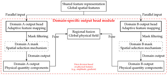
Figure 4. Parallel domain heads: global features → masked regional outputs → fused field $\widehat{u}(\mathbf{x},t)$.

Global features from SIREN are routed in parallel to Domain A and Domain B heads, each restricted by a spatial mask derived from amplitude and gradient thresholds. Domain A resolves high-gradient cores; Domain B handles smooth peripheries. Masks enforce disjoint support, eliminating cross-talk, while the fusion layer reassembles regional predictions into a single, continuous complex wavefield.

2.5. Domain Fusion and Complex Assembly

To maintain boundary continuity of the Complex Optical Wavefield, the fusion layer adopts a distance-weighted kernel to combine domain-specific complex outputs. The mathematical formulation is:

$$\begin{array}{c}\hfill {\widehat{u}}_{\mathrm{fusion}}\left(\mathbf{x}\right)=w_A\left(\mathbf{x}\right)·{\widehat{u}}_A\left(\mathbf{x}\right)+w_B\left(\mathbf{x}\right)·{\widehat{u}}_B\left(\mathbf{x}\right)\end{array}$$

(1)

where: $w_A\left(\mathbf{x}\right)=exp(-\lambda ·d(\mathbf{x},\partial {\Omega }_A))$,  $w_B\left(\mathbf{x}\right)=1-w_A\left(\mathbf{x}\right)$ ($\lambda =0.1$, a calibrated smoothing coefficient); $d(\mathbf{x},\partial {\Omega }_A)$ is the Euclidean distance from spatial coordinate $\mathbf{x}$ to the core-edge boundary ($\partial {\Omega }_A$); $w_A+w_B=1$ ensures no energy distortion, preserving the amplitude–phase coupling of the Complex Optical Wavefield. The exponential weight function realizes smooth boundary transition; it prioritizes ${\widehat{u}}_A$ (high-detail) in the core, ${\widehat{u}}_B$ (noise-robust) in the edge, and blends weights near the boundary to eliminate discontinuities.

Figure 5 illustrates the core process of the domain fusion module integrating domain-specific outputs to construct a global physical field.

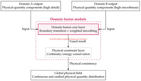
Figure 5. Domain fusion module: Fusion of Domain A (high-detail) and Domain B (smooth) outputs via boundary-weighted smoothing and physical constraints, yielding a continuous global field $\widehat{u}(\mathbf{x},t)$.

Region-specific outputs enter the fusion layer in parallel. A confidence-weighted kernel blends the two fields across their boundary, while phase-gradient and energy-conservation constraints eliminate discontinuities. The result is a single, globally consistent complex wavefield that preserves local detail and obeys physical laws.

2.6. Multi-Layer Learnable Diffraction Propagation

Figure 6 shows the core workflow of the multi-layer learnable diffraction propagation module, a hybrid “physical model-framework, learnable parameters-essence” design that maps the domain-fused initial field to the observation-matching reconstructed wavefield, acting as DdONN’s key physics-driven component bridging domain fusion and data alignment.

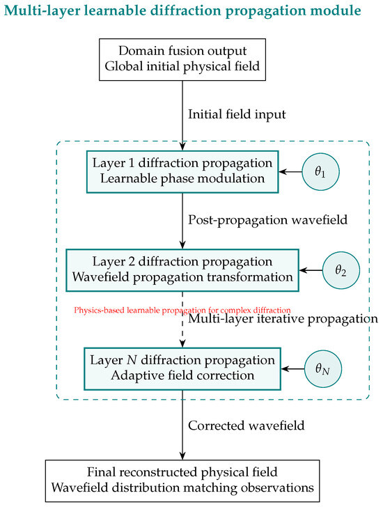
Figure 6. Learnable diffraction cascade: initial field → N phase–propagation layers → observation-matched $\widehat{u}(\mathbf{x},t)$.

The domain-fusion output ${\widehat{u}}_0(\mathbf{x},t)$ is propagated through N learnable diffraction layers. Each layer k applies a parameterized phase screen ${\theta }_k$ and a physical diffraction kernel, producing ${\widehat{u}}_k={\mathcal{D}}_{{\theta }_k}\left[{\widehat{u}}_{k-1}\right]$. The cascade progressively corrects unknown perturbations while respecting diffraction physics, yielding a final field ${\widehat{u}}_N(\mathbf{x},t)$ that simultaneously fits observations and satisfies conservation laws.

2.7. Loss Function Design

Figure 7 illustrates the overall framework and integration process of the loss function module, intuitively reflecting the constraint logic of data–physics dual-driven modeling.

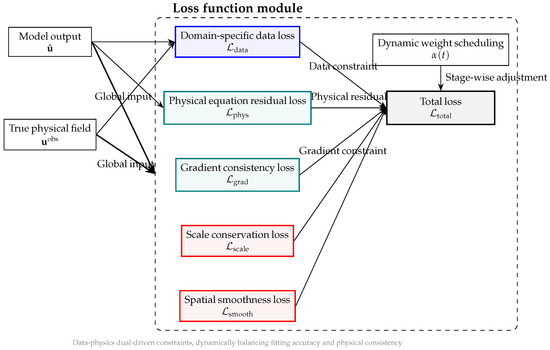
Figure 7. Loss composition: data, residual, gradient, scale and smoothness terms driven by dynamic weight $\alpha \left(t\right)$.

The total loss

$${\mathcal{L}}_{\mathrm{total}}={\mathcal{L}}_{\mathrm{data}}+\alpha \left(t\right)\left({\mathcal{L}}_{\mathrm{phys}}+{\mathcal{L}}_{\mathrm{grad}}+{\mathcal{L}}_{\mathrm{scale}}+{\mathcal{L}}_{\mathrm{smooth}}\right)$$

balances data fidelity with physical priors. ${\mathcal{L}}_{\mathrm{data}}$ uses region-aware masks to weight high-gradient cores more heavily; ${\mathcal{L}}_{\mathrm{phys}}$ penalizes NLSE residuals; ${\mathcal{L}}_{\mathrm{grad}}$ enforces phase-gradient continuity; ${\mathcal{L}}_{\mathrm{scale}}$ and ${\mathcal{L}}_{\mathrm{smooth}}$ constrain global energy and suppress noise. The schedule $\alpha \left(t\right)\in [0,1]$ starts at 0 for data-dominated learning and rises monotonically to impose physical consistency, ensuring high-precision, physically self-consistent reconstructions.

2.8. Backpropagation Optimization and Phase Screen Parameter Learning

Figure 8 illustrates the overall framework of the backpropagation optimization module and the update process of learnable parameters, intuitively reflecting the core logic of the model’s iterative parameter optimization through gradient feedback.

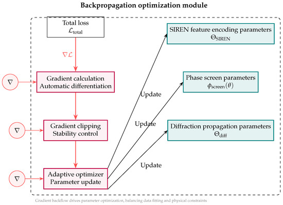
Figure 8. Gradient flow: $\nabla {\mathcal{L}}_{\mathrm{total}}\to$ optimizer → phase, SIREN, and diffraction parameters.

The gradient $\nabla {\mathcal{L}}_{\mathrm{total}}$ is back-propagated through an Amos optimizer [23] to update the shared SIREN encoder ${\Theta }_{\mathrm{SIREN}}$, the phase screens ${\varphi }_{\mathrm{screen}}\left(\theta \right)={\varphi }_{\mathrm{base}}+\Delta \varphi \left(\theta \right)$, and the diffraction-layer parameters ${\Theta }_{\mathrm{diff}}$. Here, ${\varphi }_{\mathrm{base}}$ is a fixed, pre-computed phase term derived from the Fresnel diffraction physical model—its value is determined by the spatial grid step, propagation distance, and initial wavelength before training. It encodes the ideal phase evolution of the wavefield in a disturbance-free environment, serving as the physical anchor to avoid unconstrained parameter learning. In contrast, $\Delta \varphi \left(\theta \right)$ (learnable correction term) corresponds to the trainable parameter in the Fourier diffraction layer, which specifically models unknown system perturbations or aberrations (e.g., slight inhomogeneities of the propagation medium, residual errors from numerical discretization of the diffraction kernel). This “physical base + learnable correction” design balances interpretability and adaptability, ensuring the reconstructed wavefield adheres to fundamental propagation laws while fitting observed data.

A dynamic weight $\alpha \left(t\right)$ balances data and physics contributions, while gradient clipping and weight decay ensure stable convergence. The composite phase-screen design retains physical interpretability while correcting scenario-specific aberrations.

3. Implementation Logic of Key Modules

This section introduces the core implementation mechanisms of DdONN-PINNs, including the overall architecture, feature encoding, physical propagation modeling, and training optimization strategies. All modules are implemented based on PyTorch, and the complete source code and details have been publicly released (see Figshare (DOI: https://doi.org/10.6084/m9.figshare.30384433)).

3.1. Overall Architecture of DdONN

DdONN is designed for the spatial heterogeneity of wavefields, adopting a three-layer structure of global shared encoding–regional domain-specific adaptation–physical propagation coupling. The pseudocode is as Listing 1.

Listing 1. Pseudocode for the main structure of DdONN.

Here, feature_extractor extracts continuous wavefield features; domain_heads model the characteristics of high-frequency core regions and low-frequency edge regions, respectively; and diffraction_layers serve as physical propagation modules to ensure that the output complex wavefield conforms to wave laws. The outputs of the two regions are dynamically fused via masks to guarantee boundary continuity.

3.2. SIREN Encoding Module

DdONN employs SIREN as the shared encoder, which is suitable for modeling high-frequency interference and phase variations in continuous fields. The sinusoidal activation function provides richer spectral response capability, and weight initialization adopts the SIREN-recommended strategy to ensure training stability, see Listing 2.

Listing 2. Structure of the SIREN feature extractor.

This module outputs a unified high-dimensional feature tensor, which is used by domain-specific output heads to map the real and imaginary parts of complex amplitudes, respectively.

3.3. Fourier Diffraction Propagation Modeling

To align domain-specific reconstruction results with free-space propagation, DdONN integrates a Fourier diffraction propagation layer, see Listing 3.

Listing 3. Pseudocode for the Fourier propagation layer.

The propagation kernel is derived from the Fresnel model, where wavelength and phase_screen are learnable parameters. These parameters are used to correct medium perturbations and model errors, implementing a fusion mechanism of physical model anchoring + data-driven compensation.

3.4. Training Strategy and Physical Constraints

During training, DdONN adopts a data–physics dual-driven mechanism, optimizing through dynamic fusion of data fitting errors and wave equation residuals. To address the issue of training stagnation caused by local minima—especially in the middle stage when physical constraints start to take effect—we introduce the Stochastic Gradient Descent with Warm Restarts (SGDR) strategy [24] to adjust the learning rate. This strategy periodically resets the learning rate to a higher initial value, which helps the model escape local minima while maintaining the convergence trend of the loss function. The optimization process is as Listing 4.

Listing 4. Pseudocode for the main training loop.

Here, the data loss assigns higher weights to high-frequency core regions via spatial masks; the physical term uses NLSE residuals to guide the convergence direction; the scheduling factor $\alpha \left(t\right)$ smoothly increases from 0 to 1 from the early to late training stages, enabling progressive optimization from data-driven fitting to physical consistency.

In summary, DdONN extracts continuous wavefield features through the SIREN encoder, adapts to regional differences using a domain-specific structure, introduces learnable Fourier propagation layers to model physical mechanisms, and balances data and physical terms via dynamic loss scheduling. This architecture exhibits strong interpretability and physical consistency, making it suitable for high-precision reconstruction tasks of complex optical fields.

4. Experimental Validation and Result Analysis

To rigorously benchmark DdONN-PINNs, we reconstruct rogue-wave solutions of the NLSE. These waves exhibit steep crests, pronounced spatial heterogeneity, and multi-scale interference—demanding both numerical accuracy and NLSE compliance. We address four questions: (1) amplitude and phase accuracy under noise; (2) NLSE and energy-conservation fidelity; (3) impact of domain decomposition and sinusoidal activation against ONN-PINNs without regions and DdONN-PINNs with ReLU; (4) robustness at noise levels $\sigma =0.01$, $0.05$, $0.10$.

4.1. Experimental Parameter Settings

Experimental parameters were selected via grid-search pre-studies and grouped by function. Training, structural, physical, and loss-function settings are listed in Table 1, Table 2, Table 3, and Table 4, respectively.

Table 1. Training parameters.

Parameter	Value	Purpose
Epochs	3000	total training length
Initial LR	$3\times {10}^{-4}$	cosine decay to $1\times {10}^{-7}$
Weight decay	$1\times {10}^{-5}$	regularization
Warm-up	100 epochs	data-loss only
$\alpha \left(t\right)$ ramp	500 epochs	0$\to$1 linear
Seed	42	reproducibility

Note: LR denotes learning rate.

Table 2. Model structure parameters.

Parameter	Value	Description
Spatial grid	$64\times 64$	Rogue wave range: $x\in [-5,5]$, $y\in [-3,3]$
Hidden dim	512	Balances expressiveness/cost
SIREN layers	4 (3 hidden)	Sinusoidal activation for high-frequency features
Diffraction layers	2 series	$dz=0.5$ (near), $1.5$ (far)
Complex conv kernel	$3\times 3$	Smoothing; padding = 1 (size-conserving)

Table 3. Physical modeling parameters.

Parameter	Value/Range	Description
Wavelength	1.0 (learnable)	Init = 1.0, adaptively adjusted
Core mask range	$\left|x\right|<3$, $\left|y\right|<1.5$	High-gradient regions
Noise $\sigma$	0.05 (main); 0.01 0.1	Measurement noise; robustness testing range
Grid step $dx$	$0.156$	From x-range/sampling

Table 4. Loss function parameters.

Parameter	Value	Description
Domain data loss weights	1.5 (core), 1.0 (edge)	Prioritize key structures
Phase smoothness coeff	$0.1$	Balance phase continuity
gPINN gradient weight	$0.1$	Enhance residual smoothness
Scale conservation weight	$0.2$	Control amplitude deviation

Technical notes: Training parameters (learning rate, weight decay) were optimized via grid search to balance convergence speed and stability. Model structure parameters match wavefield complexity, with 512-dimensional hidden layers sufficient to capture rogue wave high-frequency components. For physical parameters, the core region mask is based on real wavefield priors, and noise levels reference actual optical measurement scenarios. Loss function parameters were adjusted using the control variable method to prevent dominance of a single optimization objective.

4.2. Governing Equation for Rogue Wave Evolution

Rogue wave generation and propagation in experiments are governed by the NLSE, with its normalized 2D form:

$$i{\displaystyle \frac{\partial u}{\partial t}}+{\displaystyle \frac{1}{2}}{\nabla }^{2}u+{\left|u\right|}^{2}u=0$$

(2)

where $u(\mathbf{x},t)=A(\mathbf{x},t)e^{i\varphi (\mathbf{x},t)}$ is the complex wavefield; i is the imaginary unit; ${\nabla }^2={\displaystyle \frac{{\partial }^2}{\partial x^2}}+{\displaystyle \frac{{\partial }^2}{\partial y^2}}$ is the 2D Laplacian. The second-order derivative term describes dispersion, while the nonlinear term ${\left|u\right|}^{2}u$ models self-focusing—critical for energy aggregation in rogue waves.

This equation forms the core of the physical constraint loss ${\mathcal{L}}_{\mathrm{phys}}$, requiring the reconstructed wavefield $\widehat{u}$ to satisfy:

$${\mathcal{L}}_{\mathrm{phys}}=\mathbb{E}\left[{∥i{\displaystyle \frac{\partial \widehat{u}}{\partial t}}+{\displaystyle \frac{1}{2}}{\nabla }^2\widehat{u}+{\left|\widehat{u}\right|}^2\widehat{u}∥}^2\right]$$

(3)

ensuring reconstructed results conform to the physical laws of wavefield evolution.

4.3. Experimental Environment and Evaluation Metrics

Experiments were conducted on an Intel(R) Core(TM) i9-10885H CPU with 32 GB RAM (Intel Corporation, Santa Clara, CA, USA), using Python 3.10.18, Matplotlib 3.10.0, Numpy 2.2.5, Scipy 1.15.3, and PyTorch 2.5.1.

Evaluation metrics are categorized into three types:

• Numerical accuracy: Amplitude Mean Squared Error, ${\mathrm{MSE}}_A=\mathbb{E}\left[|\widehat{A}-A_{\mathrm{true}}{|}^2\right]$ and Phase Mean Squared Error, ${\mathrm{MSE}}_{\varphi }=\mathbb{E}\left[|\widehat{\varphi }-{\varphi }_{\mathrm{true}}{|}^2\right],\mathrm{where}\varphi =argu,$ quantifying numerical deviation from the true field, where ${\varphi }_i$ is obtained directly from the standard library function for complex phase.
• Physical consistency: Mean NLSE residual $\mathbb{E}\left[|\mathcal{N}[\widehat{u}]|\right]$ and Mean residual gradient $\mathbb{E}\left[|\nabla ·\mathcal{N}[\widehat{u}]|\right]$, evaluating compliance with physical laws.
• Robustness: Noise sensitivity $S={\displaystyle \frac{{\mathrm{MSE}}_A\left({\sigma }_i\right)-{\mathrm{MSE}}_A\left({\sigma }_j\right)}{{\sigma }_i-{\sigma }_j}}$, measuring MSE growth rate with noise level $\sigma$ (smaller values indicate stronger robustness).

4.4. Experimental Results and Analysis

We first present the performance of DdONN-PINNs at a noise level of $\sigma =0.05$, then compare it with ONN-PINNs variants, and finally present robustness results across noise levels.

4.4.1. Domain Decomposition, Residuals, and Point Errors

Figure 9 validates DdONN-PINNs’ performance in NLSE rogue wave reconstruction across three key aspects: spatial domain decomposition, physical consistency, and reconstruction accuracy.

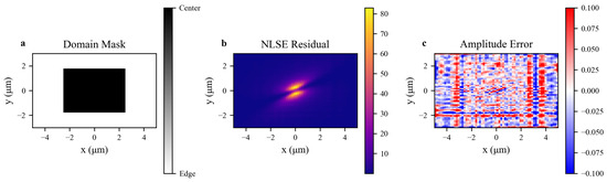
Figure 9. Spatial validation of DdONN-PINNs for NLSE rogue-wave reconstruction. (a) Domain mask: black = high-gradient core; white = low-gradient edge. (b) NLSE residual $\left|\mathcal{N}\right[\widehat{u}\left]\right|$: concentrated in the core, confirming targeted physical constraints. (c) Amplitude error map: errors within $\pm 0.1$ and spatially uniform, demonstrating balanced core-edge accuracy.

Figure 9a illustrates the decomposition strategy. This strategy applies strong NLSE constraints to the core and smoothness constraints to the edge, enabling differentiated multi-scale modeling.

Figure 9b shows that the residuals concentrate in the high-dynamic core and near-zero in the edge domain, reflecting synergies between domain decomposition and physical constraints.

Figure 9c shows that the overall error stays within $\pm 0.1$, with minimal core-edge discrepancy—verifying that domain decomposition balances fitting difficulty in high-gradient regions and stability in low-gradient regions, unifying accuracy and robustness.

In general, these results validate the domain decomposition–physical constraint synergistic mechanism, supporting DdONN-PINNs’ advantages in nonlinear wavefield modeling.

4.4.2. Rogue Wave Reconstruction

Figure 10 validates DdONN-PINNs’ robustness in wavefield reconstruction under noise via amplitude (a–c) and phase (d–f) comparisons: true field → noisy input → reconstructed result, highlighting noise suppression and feature recovery capabilities.

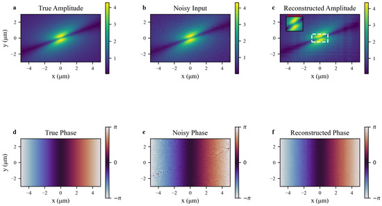
Figure 10. Amplitude (top) and phase (bottom) reconstruction of the NLSE rogue wave. (a,d) Ground truth. (b,e) Noisy input ($\sigma =0.05$). (c,f) DdONN-PINNs reconstruction. Insets in (c): $2\times 1$ $\mathsf{\mu }$m peak zoom, showing accurate recovery of steep gradients and continuous phase fronts despite noise.

True amplitude (a) exhibits the rogue wave’s high-energy double-lobe core with hierarchical spatial distribution, reflecting nonlinear evolution dynamics. Noisy amplitude (b) introduces background granular artifacts, while the core retains structure—mimicking real measurements where signal-dominated regions resist noise better. Reconstructed amplitude (c) suppresses background noise, matches the true core’s double-lobe structure, and restores edge smoothness. This stems from domain decomposition: NLSE constraints in the core preserve nonlinear features, while edge smoothness constraints filter noise, balancing structure preservation and artifact suppression.

True phase (d) shows continuous gradients from $-\pi$ to $\pi$, a hallmark of physical consistency. Noisy phase (e) suffers local fluctuations, disrupting continuity—a key challenge given phase’s noise sensitivity. Reconstructed phase (f) corrects fluctuations and recovers smooth gradients, enabled by NLSE constraints + phase smoothness loss; NLSE enforces amplitude-phase coupling for physical rationality, while smoothness loss suppresses non-physical mutations.

These results confirm DdONN-PINNs’ anti-noise strengths, rooted in domain decomposition-driven multi-constraint synergy; the core prioritizes NLSE constraints for physical accuracy, the edge uses smoothness constraints to suppress noise. This balances noise resistance, physical consistency, and robustness—critical for high-precision wavefield reconstruction in noisy scenarios.

4.4.3. Loss Curves

Figure 11 illustrates the multi-constraint training dynamics of DdONN-PINNs, showing staged evolution of global loss (a) and refined convergence of auxiliary constraints (b), revealing progressive optimization of fitting accuracy, physical consistency, and feature regularity.

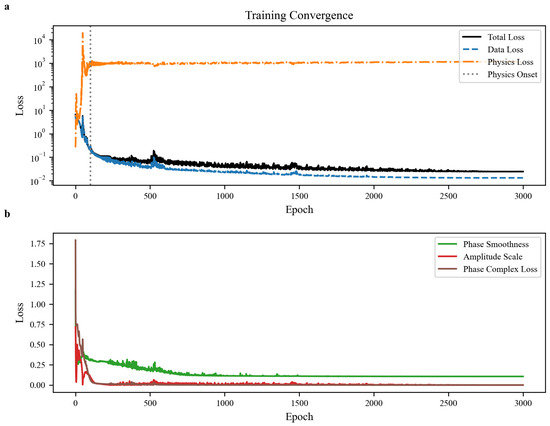
Figure 11. Training convergence of DdONN-PINNs: (a) total loss and its data/physics components; (b) auxiliary phase-smooth and scale losses.

In Figure 11a exhibits a two-stage convergence: data-driven initialization → physical constraint fine-tuning. Within 200 epochs, data loss dominates the rapid decline, as the model approximates noisy observations to construct initial wavefield distributions, while high physical loss indicates deviation from NLSE. Post-activation of physical constraints, physical loss converges gradually, aligning outputs with nonlinear evolution laws. Data loss continues to decrease but at a slower rate, reflecting synergistic optimization where physical constraints correct apparent deviations. Final stabilization of total loss confirms complementarity of the ”data fitting-physical constraint” dual architecture.

Figure 11b details auxiliary constraints refining physical features. Phase smoothness loss drops rapidly early and stabilizes at ∼0.2, indicating suppression of non-physical fluctuations and recovery of continuous phase gradients (consistent with Figure 10 phase continuity). Amplitude scale loss converges quickly and stabilizes at near-zero, verifying accurate energy conservation. Their rapid convergence reveals hierarchical optimization: phase constraints repair local mutations, amplitude constraints calibrate global energy, jointly supporting physical consistency.

Loss evolution follows apparent fitting → law alignment → feature refinement: data loss enables rapid approximation of observations; physical loss anchors NLSE laws to correct deviations; auxiliary constraints refine local/global features. This hierarchical mechanism avoids overfitting and convergence inertia, unifying fitting accuracy and physical consistency in complex wavefield reconstruction.

4.4.4. Residual Contours and Their Correlation with Gradients

Figure 12 examines the distribution of physical residuals in DdONN-PINNs reconstructions, via residual spatial patterns (a) and their quantitative correlation with physical quantities (b), validating targeted constraint effectiveness and residual interpretability.

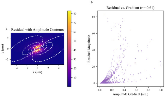
Figure 12. Residual correlation analysis for NLSE rogue-wave reconstruction. (a) NLSE residual $\left|\mathcal{N}\right[\widehat{u}\left]\right|$ overlaid with amplitude contours (dashed white lines); high residuals concentrate in high-gradient regions. (b) Scatter plot of residual magnitude vs. amplitude gradient magnitude (Pearson $r=0.61$), confirming residuals align with regions of strong spatial variation and high physical complexity.

Figure 12a shows residuals $\left|\mathcal{N}\right[\widehat{u}\left]\right|$ overlaid with amplitude contours. High residuals localize to high-gradient regions (dense contours), while edge regions with low amplitude/gradient exhibit minimal residuals. This confirms the model’s design logic: physical constraints focus on key regions—high-gradient areas naturally accumulate residuals due to fitting difficulty, while low-gradient regions satisfy constraints more easily. Residuals here are not random but tied to inherent wavefield physics, guiding adaptive sampling of high-residual regions for targeted optimization.

Figure 12b quantifies this relationship, with a significant positive correlation ($r=0.61$) between residuals and amplitude gradients. Higher gradients indicate complex structures, where balancing data fitting and physical laws is harder—explaining elevated residuals. Lower gradients correspond to simpler physics and reduced residuals. This aligns with DdONN-PINNs’ domain decomposition; region-specific heads use complex mappings for high-gradient areas, while loss functions weight high-residual regions more heavily, enabling “precise constraint in complex regions, stable fitting in simple ones”.

In summary, residuals strongly correlate with wavefield physical features, confirming their interpretability. DdONN-PINNs naturally focuse constraints on high-gradient regions, synergizing with residual-gradient enhancement mechanisms to ensure reconstruction consistency.

4.5. Quantitative Result Comparison and Analysis

At a fixed noise level of $\sigma =0.05$, three comparative experiments were designed: DdONN-PINNs, a non-domain-decomposition variant (NoDdONN-PINNs), and a ReLU-activated variant (ReLUDdONN-PINNs) to analyze the impacts of domain decomposition and activation functions on wavefield reconstruction.

Furthermore, we denote the Mean Error of Amplitude as ${\mathrm{ME}}_A$, the Mean of the Physical Residual as ${\mathrm{M}}_{\mathrm{Phys}.\mathrm{Res}}$, and the Standard Deviation of the Physical Residual as ${\mathrm{Std}}_{\mathrm{Phys}.\mathrm{Res}}$.

Table 5 and Figure 13 show synergistic effects of activation functions and domain decomposition. For reconstruction accuracy, activation function properties drive significant divergence: ReLUDdONN-PINNs’ Amp MSE is $3.31\times$ that of DdONN-PINNs and $6.2\times$ that of NoDdONN-PINNs, as ReLU’s piecewise linearity fails to capture smooth, periodic wavefield variations—introducing large errors in steep-gradient crests and interference details. Phase MSE contrasts are starker: ReLUDdONN-PINNs’ value ($3.18\times {10}^{-3}$) far exceeds DdONN-PINNs’ ($5.86\times {10}^{-4}$, $5.43\times$ lower) and NoDdONN-PINNs’ ($1.68\times {10}^{-3}$, $1.89\times$ lower), verifying sinusoidal activation’s inherent advantage in modeling phase continuity versus ReLU’s hard saturation, which causes phase jumps even with domain decomposition.

Table 5. Quantitative comparison of NLSE rogue wave reconstruction.

Model	${\mathbf{MSE}}_{\mathit{A}}$	${\mathbf{MSE}}_{\mathit{\varphi }}$	${\mathbf{ME}}_{\mathit{A}}$	${\mathbf{M}}_{\mathbf{Phys}.\mathbf{Res}}$	${\mathbf{Std}}_{\mathbf{Phys}.\mathbf{Res}}$
DdONN-P	$2.94\times {10}^{-3}$	$5.86\times {10}^{-4}$	$2.90\times {10}^{-5}$	$3.10\times {10}^0$	$8.18\times {10}^0$
NoDdONN-P	$1.57\times {10}^{-3}$	$1.68\times {10}^{-3}$	$2.40\times {10}^{-5}$	$3.07\times {10}^0$	$7.96\times {10}^0$
ReLUDdONN-P	$9.74\times {10}^{-3}$	$3.18\times {10}^{-3}$	$1.04\times {10}^{-3}$	$3.05\times {10}^0$	$7.62\times {10}^0$

Abbreviations: -P = -PINNs; ${\mathrm{ME}}_A$ = Amplitude Mean Error.

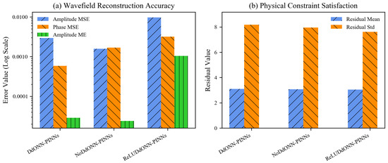
Figure 13. Quantitative performance comparison of three variants: (a) reconstruction accuracy; (b) physical residual statistics. Results reveal impacts of domain decomposition and activation functions on modeling fidelity.

For physical consistency, all models show comparable mean residuals ($\sim 3.05\times {10}^0$–$3.10\times {10}^0$) and standard deviations ($\sim 7.62\times {10}^0$–$8.18\times {10}^0$), indicating ReLU variants still satisfy basic wave evolution laws. However, residual spatial patterns reveal that ReLUDdONN-PINNs’ high residuals concentrate in high-gradient crests—its overall mean reflects large residuals in key regions + small residuals in flat regions, contrasting with DdONN-PINNs’ focus on reducing residuals in critical areas.

Regarding the learnable wavelength parameter (Table 3), its final learned value ($1.02$) deviates slightly from the initial $1.0$. This deviation is attributed to numerical discretization error correction (e.g., grid sampling and diffraction kernel approximation biases) rather than physical model adjustment, as the ≤2% variation maintains compliance with NLSE physics.

In summary, matching domain decomposition + activation function properties is critical. DdONN-PINNs achieve high detail precision and physical robustness via domain-specific modeling + sinusoidal activation. ReLUDdONN-PINNs’ bottleneck confirms ReLU’s inherent mismatch with wavefields’ smooth periodicity—domain decomposition alone cannot replace sinusoidal activation in wave system modeling, providing guidance for activation function selection.

4.6. Robustness Verification

Table 6 summarizes DdONN-PINNs’ numerical accuracy, physical consistency, and robustness metrics across different noise levels, with Figure 14 further characterizing its noise robustness.

Table 6. Evaluation metrics under different noise levels.

Evaluation Metric	$\mathit{\sigma }=0.01$	$\mathit{\sigma }=0.05$	$\mathit{\sigma }=0.10$
${\mathrm{MSE}}_A$ (Amplitude MSE)	0.002303	0.002936	0.004738
${\mathrm{MSE}}_{\varphi }$ (Phase MSE)	0.000374	0.000586	0.001646
${\mathrm{M}}_{\mathrm{Phys}.\mathrm{Res}}$ (Residual Mean)	$3.0933\times {10}^0$	$3.0996\times {10}^0$	$3.1095\times {10}^0$
Mean Residual Gradient	$0.0\times {10}^0$	$0.0\times {10}^0$	$0.0\times {10}^0$
Amp Mean Error	0.000065	0.000029	0.000115
Learned center_phi	0.000115	0.000022	0.000454
Learned edge_phi	−0.000586	0.001290	0.001921
Noise Sensitivity (S)
Low-noise interval ($\sigma =0.01\to 0.05$)	0.0158
High-noise interval ($\sigma =0.05\to 0.10$)	0.0360
Full interval ($\sigma =0.01\to 0.10$)	0.0271

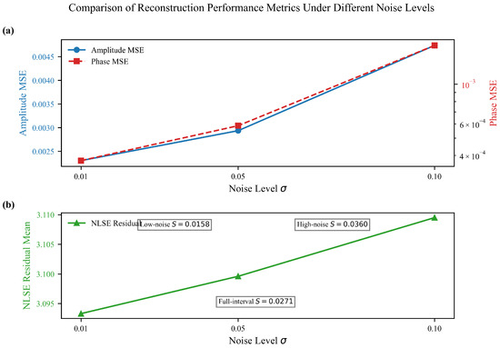
Figure 14. Noise robustness of DdONN-PINNs across $\sigma \in \{0.01,0.05,0.10\}$. (a) Amplitude MSE (blue) rises monotonically with mild nonlinearity; phase MSE (red) increases steadily, highlighting phase sensitivity to noise. (b) Mean NLSE residual (green) shows slight monotonic growth yet remains stable, confirming sustained physical consistency. Noise sensitivity S (full-interval $S=0.0271$, low-noise $S=0.0158$, high-noise $S=0.0360$) underscores robust amplitude recovery with interval-dependent error growth.

Table 6 shows that ${\mathrm{MSE}}_A$ increases monotonically with noise, from $2.30\times {10}^{-3}$ ($\sigma =0.01$) to $4.74\times {10}^{-3}$ ($\sigma =0.10$), reflecting a systematic degradation in amplitude reconstruction accuracy. In contrast, ${\mathrm{MSE}}_{\varphi }$ rises from $3.74\times {10}^{-4}$ to $1.65\times {10}^{-3}$, growing at a faster rate, which is attributed to the high-frequency nature of phase information—noise amplifies errors through the phase unwrapping process, highlighting the high sensitivity of phase reconstruction to measurement noise.

In terms of physical consistency, the mean NLSE residual remains stable across all noise levels with only minor fluctuations (from $3.0933\times {10}^0$ to $3.1095\times {10}^0$, coefficient of variation $<0.5\%$), indicating that the model’s physical constraint mechanisms (including NLSE residual loss and adaptive sampling) effectively resist noise interference, ensuring the reconstructed wavefield complies with the NLSE. Notably, the mean residual gradient remains $0.0\times {10}^0$ throughout, an ideal result reflecting that the gradient constraint successfully enhances the spatial continuity of physical residuals, avoiding noise-induced local mutations in residuals and further verifying the role of gradient consistency constraints in ensuring compliance with physical laws.

The full-interval noise sensitivity $S=0.0271$ indicates a low growth rate of amplitude error with noise level, demonstrating good overall noise resistance. Further analysis reveals that sensitivity varies across intervals. It is $0.0158$ in the low-noise interval ($\sigma =0.01\to 0.05$) and $0.0360$ in the high-noise interval ($\sigma =0.05\to 0.10$), reflecting the model’s behavior under different noise intensities—under low noise, interference is mitigated by precise fitting in core regions; under high noise, error diffusion is suppressed by constraints in edge regions, though sensitivity still increases. This fitting-constraint dynamic confirms the synergistic effect of the domain decomposition strategy and physical constraints, supporting reconstruction stability in medium- to high-noise scenarios.

Figure 14 clarifies the trends of these metrics: (a) ${\mathrm{MSE}}_A$ (blue line) exhibits a monotonic nonlinear increase with noise level $\sigma$, while ${\mathrm{MSE}}_{\varphi }$ (red line) rises steadily with $\sigma$, highlighting the inherent sensitivity of phase to noise. The quantified noise sensitivity S (full-interval $S=0.0271$, low-noise $S=0.0158$, high-noise $S=0.0360$) confirms interval-dependent amplitude error growth, where high-noise sensitivity increases—attributed to the trade-off between domain-specific fitting and noise-induced interference. (b) The mean NLSE residual (green line) shows slight monotonic growth yet remains stable, verifying the effectiveness of constraint mechanisms in suppressing noise-induced error diffusion while maintaining physical consistency.

In summary, the experimental results confirm three key advantages of the DdONN-PINNs model under noise interference. First, amplitude reconstruction exhibits strong robustness, meeting the accuracy requirements for amplitude information in engineering applications; second, physical constraint mechanisms effectively ensure the physical rationality of the wavefield, which is not significantly affected by noise levels; finally, the synergistic effect of the domain decomposition strategy and gradient constraints provides a feasible path for high-precision reconstruction of complex wavefields in noisy environments.

4.7. Ablation Study

We conducted ablation experiments on Dynamic Weight Scheduling and Auxiliary Physical Constraints, respectively. All experiments were carried out with identical hyperparameters, including network architecture, learning rate, noise level ($\sigma =0.05$), and total training epochs (3000). For performance evaluation, three key metrics were adopted: ${\mathrm{MSE}}_A$, ${\mathrm{MSE}}_{\varphi }$, and ${\mathrm{M}}_{\mathrm{Phys}.\mathrm{Res}}$

4.7.1. Dynamic Weight Scheduling

To validate the fixed linear schedule of $\alpha \left(t\right)$ against adaptive weighting mechanisms, we compare three strategies—fixed linear $\alpha$, gradient-norm adaptive $\alpha$, and loss-ratio adaptive $\alpha$—under consistent experimental conditions, isolating the impact of $\alpha \left(t\right)$ on performance.

The fixed linear strategy increases $\alpha$ from 0 to 1 over 500 epochs after a 100-epoch warmup; the gradient-norm strategy uses $\alpha = \parallel \nabla L_{\mathrm{phys}}\parallel /(\parallel \nabla L_{\mathrm{data}}\parallel + \parallel \nabla L_{\mathrm{phys}}\parallel )$; the loss-ratio strategy adopts $\alpha =L_{\mathrm{data}}/(L_{\mathrm{data}}+L_{\mathrm{phys}})$.

Table 7 and Figure 15 evaluate different $\alpha$ scheduling strategies. Adaptive $\alpha$ improves amplitude MSE ($0.001359$ vs. fixed linear $\alpha$’s $0.002936$) but compromises phase fidelity (${\mathrm{MSE}}_{\varphi }=0.001595$ vs. $0.000586$) and physical consistency (learned wavelength $0.9887$ vs. $0.9957$). Adaptive $\alpha$ (Loss Ratio) further exacerbates phase error while preserving residual similarity to fixed linear $\alpha$, highlighting trade-offs between reconstruction accuracy and physical constraint adherence.

Table 7. Quantitative comparison of different $\alpha$ scheduling strategies.

Strategy	${\mathbf{MSE}}_{\mathit{A}}$	${\mathbf{MSE}}_{\mathit{\varphi }}$	Mean Residual	Amplitude Mean Error	Learned Wavelength
Fixed Linear $\alpha$	0.002936	0.000586	$3.0996\times {10}^0$	0.000029	0.9957
Adaptive $\alpha$ (Gradient Norm)	0.001359	0.001595	$3.0854\times {10}^0$	0.000046	0.9887
Adaptive $\alpha$ (Loss Ratio)	0.001888	0.002286	$3.0918\times {10}^0$	0.000067	0.9757

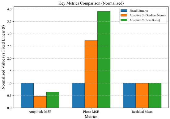
Figure 15. Training dynamics and performance of different $\alpha$ scheduling strategies.

4.7.2. Auxiliary Physical Constraints

To validate the necessity of auxiliary physical constraints in the total loss, we conduct ablation experiments by systematically removing key components—specifically $L_{\mathrm{grad}}$ and $L_{\mathrm{scale}}$—and evaluating their impact on phase accuracy and physical fidelity. These experiments use the proposed fixed linear $\alpha \left(t\right)$ schedule and maintain identical hyperparameters to isolate the effect of each constraint.

Three configurations are tested: (1) full loss (all constraints: $L_{\mathrm{phys}}+L_{\mathrm{grad}}+L_{\mathrm{scale}}+L_{\mathrm{smooth}}$); (2) without $L_{\mathrm{grad}}$; (3) without $L_{\mathrm{scale}}$. Performance is evaluated using four key metrics to comprehensively reflect wavefield reconstruction quality: ${\mathrm{MSE}}_A$ for amplitude accuracy, ${\mathrm{MSE}}_{\varphi }$ for phase consistency, $\Delta E=|\mathbb{E}[|\widehat{u}{|}^2]-\mathbb{E}[|u_{\mathrm{true}}{|}^2]|$ for energy fidelity, and ${\mathrm{M}}_{\mathrm{Phys}.\mathrm{Res}}$ for physical compliance.

Table 8 presents the ablation results of two key auxiliary physical constraints in the full loss function, with the full loss serving as the baseline. Removing $L_{\mathrm{grad}}$ reduces the phase error $MS{E}_{\varphi }$ from $0.000586$ to $0.000438$ but increases the amplitude mean error from $0.000029$ to $0.000171$. In contrast, omitting $L_{\mathrm{scale}}$ leads to a more significant rise in amplitude mean error, to $0.001001$, and a noticeable deviation in the learned wavelength $\lambda$, from $0.995741$ to $0.969825$, while $MS{E}_{\varphi }$ decreases moderately to $0.000463$. These results confirm that $L_{\mathrm{grad}}$ and $L_{\mathrm{scale}}$ play non-trivial roles: $L_{\mathrm{grad}}$ balances phase accuracy and energy conservation, and $L_{\mathrm{scale}}$ is critical for maintaining energy fidelity and stable learning of physical parameters, justifying their inclusion and weighting in the final model.

Table 8. Ablation of auxiliary physical constraints ($L_{\mathrm{grad}}$ and $L_{\mathrm{scale}}$).

Ablation Case	${\mathit{MSE}}_{\mathit{A}}$	${\mathit{MSE}}_{\mathit{\varphi }}$	Amp Mean Err.	Res. Mean	Learned $\mathit{\lambda }$
Full Loss (Baseline)	0.002936	0.000586	0.000029	$3.0996\times {10}^0$	0.995741
W/O $L_{\mathrm{grad}}$	0.002295	0.000438	0.000171	$3.0857\times {10}^0$	0.993743
W/O $L_{\mathrm{scale}}$	0.001808	0.000463	0.001001	$3.0880\times {10}^0$	0.969825

4.8. Scaling Analysis for Higher-Resolution Wavefield Reconstruction

High-resolution sampling is critical for capturing steep-gradient features like rogue wave crests. This subsection evaluates the proposed method across $64\times 64$ and $128\times 128$ grids, analyzing how reconstruction quality and computational cost scale to validate applicability in large-scale, high-fidelity simulations.

Spatial resolution experiments investigate the effect of scaling spatial resolution (from $64\times 64$ to $128\times 128$, a $4\times$ increase in grid size) on DdONN-PINNs. As shown in Table 9 and Figure 16a, key training cost metrics—total training time, average time per epoch, and time ratio—rise by $5.5\times$, outpacing the $4\times$ grid expansion. For reconstruction performance (Table 10 and Figure 16b), amplitude MSE (Amp MSE) increases by $3.94\times$ (closely matching the $4\times$ resolution scaling), whereas phase MSE ($1.76\times$) and residual mean ($1.02\times$) exhibit smaller growth, revealing metric-dependent sensitivity to resolution. Table 11 further demonstrates that DdONN-PINNs adaptively adjust learned parameters (wavelength, center_phi, and edge_phi) to accommodate fine-grained structures at higher resolutions.

Table 9. Training cost.

Res.	Total Time	Avg per Epoch	Time Ratio
	(min)	(s)	(vs. 64 × 64)
64 × 64	16.49	0.3298	1.00
128 × 128	91.18	1.8237	5.50
4×	5.52×	5.53×	5.50×

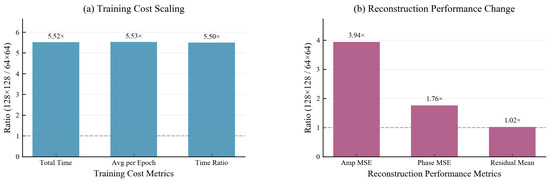
Figure 16. Resolution scaling analysis of DdONN-PINNs. (a) Training cost scaling with spatial resolution. (b) Reconstruction performance change with spatial resolution.

Table 10. Reconstruction performance of DdONN-PINNs.

Res.	Amp MSE	Phase MSE	Residual Mean
64 × 64	0.001116	0.000275	3.0748
128 × 128	0.004393	0.000483	3.1464
4×	3.94×	1.76×	1.02×

Table 11. Learned parameters of DdONN-PINNs.

Res.	Wavelength	Center_phi	Edge_phi
64 × 64	0.973789	0.001627	0.000516
128 × 128	0.975377	−0.000641	0.001316

center_phi/edge_phi = Domain-specific phase compensation offsets (core/edge regions).

5. Conclusions

To address limitations of traditional methods in reconstructing complex optical wavefields (e.g., rogue waves)—where balancing spatial heterogeneity adaptation, physical law constraints, and complex-domain modeling remains challenging—this paper proposes DdONN-PINNs. By integrating wavefield physical properties with deep learning, it achieves high-precision, physically consistent reconstruction through synergistic multi-dimensional designs.

Utilizing wavefield spatial heterogeneity—high-frequency complexity in core regions and low-frequency smoothness in edges—a SIREN shared encoder + domain-specific output heads architecture with spatial masks dynamically allocates model capacity, resolving accuracy imbalances in global fitting by a single network. Complementing this, a dual mechanism of physical process embedding + constraint enhancement is adopted: Fourier diffraction layers simulate propagation, while gradient-enhanced and adaptive sampling PINNs strengthen physical constraints for inhomogeneous fields. Physically guided loss functions, including domain-specific data loss and amplitude scale conservation terms, reinforce amplitude-phase correlations, while native complex-domain modeling directly outputs real and imaginary parts for joint optimization—with complex convolution smoothing preserving wavefield coupling that separate real–imaginary processing would disrupt.

Experiments on NLSE-described rogue wavefields show that DdONN-PINNs outperform non-domain-decomposed models and ReLU-activated variants, accurately restoring steep crests and interference fringes. Synergies of domain decomposition (focusing on high-gradient cores) and sinusoidal activation (ensuring phase continuity) enable robust modeling of complex structures.

Robustness tests confirm stable performance across noise levels; amplitude errors grow gently, physical constraints resist noise to maintain energy conservation and phase continuity, and strong residual-gradient correlations verify targeted constraint action on critical regions.

DdONN-PINNs advance complex optical wavefield reconstruction via domain adaptation + physical fusion + complex modeling, with potential applications in fiber-optic pulses and ocean waves. Future work will explore dynamic domain decomposition, efficient physical operators, and multi-modal data fusion to enhance generalization.

References

- Wetzstein, G.; Ozcan, A.; Gigan, S.; Fan, S.; Englund, D.; Soljačić, M.; Denz, C.; Miller, D.A.B.; Psaltis, D. Inference in artificial intelligence with deep optics and photonics. Nature 2020, 588, 39–47. [Google Scholar] [CrossRef]
- Hu, J.; Mengu, D.; Tzarouchis, D.C.; Edwards, B.; Engheta, N.; Ozcan, A. Diffractive optical computing in free space. Nat. Commun. 2024, 15, 1525. [Google Scholar] [CrossRef]
- Goodman, J.W. Introduction to Fourier Optics; Roberts and Company Publishers: Greenwood Village, CO, USA, 2005. [Google Scholar]
- Li, G.H.Y.; Wang, Z.; Marandi, A. Deep learning with photonic neural cellular automata. Light Sci. Appl. 2025, 14, 283. [Google Scholar] [CrossRef]
- Fu, T.; Zhang, J.; Sun, R.; Huang, Y.; Xu, W.; Yang, S.; Zhu, Z.; Chen, H. Optical neural networks: Progress and challenges. Light Sci. Appl. 2024, 13, 263. [Google Scholar] [CrossRef] [PubMed]
- Xue, Z.; Zhou, T.; Xu, Z.; Yu, S.; Dai, Q.; Fang, L. Fully forward mode training for optical neural networks. Nature 2024, 632, 280–286. [Google Scholar] [CrossRef]
- Ma, S.Y.; Wang, T.; Laydevant, J.; Wright, L.G.; McMahon, P.L. Quantum-limited stochastic optical neural networks operating at a few quanta per activation. Nat. Commun. 2025, 16, 359. [Google Scholar] [CrossRef]
- Kazanskiy, N.L.; Golovastikov, N.V.; Khonina, S.N. The Optic Brain: Foundations, frontiers, and the future of photonic artificial intelligence. Mater. Today Phys. 2025, 58, 101856. [Google Scholar] [CrossRef]
- Lin, X.; Rivenson, Y.; Yardimci, N.T.; Veli, M.; Luo, Y.; Jarrahi, M.; Ozcan, A. All-optical machine learning using diffractive deep neural networks. Science 2018, 361, 1004–1008. [Google Scholar] [CrossRef] [PubMed]
- Rahman, M.S.S.; Li, J.; Mengu, D.; Luo, Y.; Rivenson, Y.; Ozcan, A. Ensemble learning of diffractive optical networks. Light Sci. Appl. 2021, 10, 14. [Google Scholar] [CrossRef] [PubMed]
- Jagtap, A.D.; Karniadakis, G.E. Extended Physics-Informed Neural Networks (XPINNs): A Generalized Space-Time Domain Decomposition Based Deep Learning Framework for Nonlinear Partial Differential Equations. Commun. Comput. Phys. 2020, 28, 2282003. [Google Scholar] [CrossRef]
- Zhong, C.; Liao, K.; Dai, T.; Yu, X.; Xie, H.; Liu, J. Graphene/silicon heterojunction for reconfigurable phase-relevant activation function in coherent optical neural networks. Nat. Commun. 2023, 14, 6939. [Google Scholar] [CrossRef]
- Gu, Z.; Ma, Q.; Gao, X.; You, J.W.; Cui, T.J. Direct electromagnetic information processing with planar diffractive neural network. Sci. Adv. 2024, 10, eado3937. [Google Scholar] [CrossRef]
- Raissi, M.; Perdikaris, P.; Karniadakis, G.E. Physics-informed neural networks: A deep learning framework for solving forward and inverse problems involving nonlinear partial differential equations. J. Comput. Phys. 2019, 378, 686–707. [Google Scholar] [CrossRef]
- Barbulescu, R.; Ciuprina, G.; Duca, A.; Machado, P.; Silveira, L.M. Physics-informed neural networks for a highly nonlinear dynamic system. J. Math. Ind. 2025, 15, 7. [Google Scholar] [CrossRef]
- Dolea, V.; Heinlein, A.; Mishra, S.; Moseley, B. Multilevel domain decomposition-based architectures for physics-informed neural networks. Comput. Methods Appl. Mech. Eng. 2024, 429, 117116. [Google Scholar] [CrossRef]
- Chong, K.C.; Pramanik, M. Physics-guided neural network for tissue optical properties estimation. Biomed. Opt. Express 2023, 14, 2576–2590. [Google Scholar] [CrossRef]
- Trabelsi, C.; Bilaniuk, O.; Zhang, Y.; Serdyuk, D.; Subramanian, S.; Santos, J.F.; Mehri, S.; Rostamzadeh, N.; Benigo, Y.; Pal, C. Deep complex networks. In Proceedings of the International Conference on Learning Representations (ICLR) 2018, Vancouver, BC, Canada, 30 April–3 May 2018. [Google Scholar]
- Sitzmann, V.; Martel, J.N.P.; Bergman, A.W.; Lindell, D.B.; Wetzstein, G. Implicit Neural Representations with Periodic Activation Functions. In Proceedings of the 34th Conference on Neural Information Processing Systems (NeurIPS 2020), Vancouver, BC, Canada, 6–12 December 2020. [Google Scholar]
- Zhang, L.; Du, M.; Bai, X.; Chen, Y.; Zhang, D. Complex-valued physics-informed machine learning for efficient solving of quintic nonlinear Schrödinger equations. Phys. Rev. Res. 2025, 7, 013164. [Google Scholar] [CrossRef]
- McClenny, L.M.; Braga-Neto, U. Self-adaptive physics-informed neural networks. J. Comput. Phys. 2023, 471, 111712. [Google Scholar] [CrossRef]
- Yu, J.; Lu, L.; Meng, X.; Karniadakis, G.E. Gradient-enhanced physics-informed neural networks for forward and inverse PDE problems. Comput. Methods Appl. Mech. Eng. 2022, 393, 114823. [Google Scholar] [CrossRef]
- Tian, R.; Parikh, A.P. Amos: An Adam-style Optimizer with Adaptive Weight Decay towards Model-Oriented Scale. arXiv 2022, arXiv:2210.11693. [Google Scholar]
- Loshchilov, I.; Hutter, F. SGDR: Stochastic Gradient Descent with Warm Restarts. arXiv 2017, arXiv:1608.03983. [Google Scholar] [CrossRef]
Disclaimer/Publisher’s Note: The statements, opinions and data contained in all publications are solely those of the individual author(s) and contributor(s) and not of MDPI and/or the editor(s). MDPI and/or the editor(s) disclaim responsibility for any injury to people or property resulting from any ideas, methods, instructions or products referred to in the content. |
© 2025 by the authors. Licensee MDPI, Basel, Switzerland. This article is an open access article distributed under the terms and conditions of the Creative Commons Attribution (CC BY) license (https://creativecommons.org/licenses/by/4.0/).