High-Accuracy Solutions to the Time-Fractional KdV–Burgers Equation Using Rational Non-Polynomial Splines

Abstract

A non-polynomial spline is a technique that utilizes information from symmetric functions to solve mathematical or physical models numerically. This paper introduces a novel non-polynomial spline construct incorporating a rational function term to develop an efficient numerical scheme for solving time-fractional differential equations. The proposed method is specifically applied to the time-fractional KdV–Burgers (TFKdV) equation. and time-fractional differential equations are crucial in physics as they provide a more accurate description of various complex processes, such as anomalous diffusion and wave propagation, by capturing memory effects and non-local interactions. Using Taylor expansion and truncation error analysis, the convergence order of the numerical scheme is derived. Stability is analyzed through the Fourier stability criterion, confirming its conditional stability. The accuracy and efficiency of the rational non-polynomial spline (RNPS) method are validated by comparing numerical results from a test example with analytical and previous solutions, using norm errors. Results are presented in $2D$ and $3D$ graphical formats, accompanied by tables highlighting performance metrics. Furthermore, the influences of time and the fractional derivative are examined through graphical analysis. Overall, the RNPS method has demonstrated to be a reliable and effective approach for solving time-fractional differential equations.

1. Introduction

In recent years, fractional derivatives have garnered significant interest due to their capacity to capture memory effects and hereditary characteristics, which traditional integer-order derivatives cannot model. Fractional calculus extends the classical framework by permitting differentiation and integration to occur at non-integer orders, making it particularly well-suited for systems that exhibit complex or anomalous behaviors. This advanced mathematical approach provides a more nuanced and precise depiction of real-world processes, especially in contexts where non-local interactions and long-term dependencies play a critical role [1].

The versatility of fractional calculus is evident in its wide range of applications. In signal processing and dynamical systems, fractional operators enhance the modeling of systems with frequency-dependent behavior, improving precision in areas such as control theory and filtering [2]. In engineering and mechanics, fractional models offer better accuracy for systems with viscoelasticity, damping, and diffusion processes [3]. Fractional calculus also plays a critical role in solving physical problems, particularly those involving diffusion and wave propagation [4], as well as in fluid mechanics for describing non-Newtonian fluid flows [5]. Additionally, in biological modeling, fractional derivatives capture complex biological processes like population dynamics and memory effects in tissue modeling, leading to more realistic models of biological systems [6]. Several formulations of fractional derivatives have been developed, including the Riemann–Liouville, Grünwald–Letnikov, Hadamard, Weyl, Caputo, and conformable derivatives, each offering distinct advantages for mathematical modeling and analysis [7,8,9,10].

In recent times, solving FDEs numerically has become an area of great interest due to their critical role in representing complex systems. This section outlines key research that has pushed the boundaries of the field. For instance, cubic B-splines have been applied to solve the Painlevé and Bagley–Torvik equations with varying fractional derivatives [11]. Non-polynomial splines have been explored for the KdV equation with a time-fractional derivative [12], while the finite difference method has been widely used for various FDEs [13]. Furthermore, the finite element method has been effectively utilized for three-dimensional fractional differential equations [14], and the fractional-order Chelyshkov wavelet method has been employed to solve variable-order fractional equations [15]. Among the prominent techniques for tackling FDEs, the non-polynomial spline method has been extensively applied, addressing several fractional differential equations such as the fourth-order time-fractional differential equation [16], time-fractional advection-diffusion equation [17], nonlinear Schrödinger equation [18], time-fractional Burgers–Fisher equation [19], and nonlinear coupled Burgers’ equations [20]. Building on this foundation, the present study introduces a novel RNPS approach to solve the TFKdVB equation.

The TFKdVB equation incorporates a fractional temporal derivative and finds applications in various fields, including plasma wave dynamics [21], wave propagation in elastic tubes filled with viscous fluids [22], and long-wave movement in shallow waters [23]. Several numerical methods have been proposed to solve this equation, such as the Petrov–Galerkin method [24], natural transform decomposition method [25], finite difference method [26], double Laplace transform [27], spectral collocation method [28], and residual power series method [29].

This work is motivated by the need for efficient methods to solve time-fractional equations, which model complex phenomena with memory effects. The proposed RNPS method enhances accuracy and stability, addressing challenges in traditional approaches, particularly for the TFKdV equation, a key model in nonlinear wave dynamics.

The RNPS method differs from previous approaches by being the first to use a non-polynomial spline with a rational function term, instead of the commonly used exponential, hyperbolic, or trigonometric functions [8,12].

This work aims to enhance the precision and efficiency of numerical methods for time-fractional differential equations, which play a key role in modeling complex physical systems. The primary contribution is the development and application of the RNPS technique for solving the TFKdVB equation, achieving high convergence and conditional stability. The uniqueness of this approach lies in the incorporation of rational functions within the spline structure, delivering improved performance compared to standard numerical techniques. Comprehensive error analysis and comparisons validate the RNPS method, showcasing its higher accuracy and resilience, as reflected in both 2D and 3D graphical results.

The structure of this paper is as follows: Section 2 introduces the mathematical framework, detailing the general form of the TFKdV equation along with its associated initial and boundary conditions. Section 3 outlines the development of the new non-polynomial spline construction, which includes a rational function term. In Section 4, the order of convergence is determined through truncation error analysis and Taylor expansion. Section 5 demonstrates the application of the proposed numerical method to the TFKdV equation. Section 6 provides a stability analysis of the RNPS method. Section 7 presents examples with corresponding figures, tables, and a comparison of results, followed by an in-depth discussion. Lastly, Section 8 concludes with a summary of the findings, highlighting the advantages of the proposed method and its broader implications.

2. Mathematical Model

This section introduces an extended form of the TFKdVB equation, incorporating conformable fractional-order derivatives, as follows:

$$T_{\vartheta }^{\alpha }u+{\sigma }_{1}u\left(\phi ,\vartheta \right){\displaystyle \frac{\partial u\left(\phi ,\vartheta \right)}{\partial \phi }}-{\sigma }_2{\displaystyle \frac{{\partial }^{2}u\left(\phi ,\vartheta \right)}{\partial {\phi }^2}}+{\sigma }_3{\displaystyle \frac{{\partial }^{3}u\left(\phi ,\vartheta \right)}{\partial {\phi }^3}}=F\left(\phi ,\vartheta \right),0<\alpha \le 1,$$

(1)

with boundaries and initial conditions as follows:

$$\begin{array}{cc}\hfill & u\left(a,\vartheta \right)={\varphi }_1\left(\vartheta \right),\hfill \\ \hfill & u\left(b,t\right)={\varphi }_2\left(\vartheta \right),\hfill \\ \hfill & u_{\phi }\left(b,\vartheta \right)={\varphi }_3\left(\vartheta \right),\hfill \\ \hfill & u\left(\phi ,0\right)=\Psi \left(\phi \right),\hfill \end{array}$$

(2)

where ${\sigma }_1\ne 0$ and ${\sigma }_2,{\sigma }_3$ are specified positive constants and $T_{\vartheta }^{\alpha }$ denotes conformable fractional derivative defined as follows [10]:

$$T_{\vartheta }^{\alpha }u\left(\vartheta \right)=\underset{ϵ\to \infty }{lim}{\displaystyle \frac{u(\vartheta +ϵ{\vartheta }^{1-\alpha })-u\left(\vartheta \right)}{ϵ}}.$$

(3)

3. A Non-Polynomial Spline with Rational-Term Construction

This section explores a novel construction involving a non-polynomial spline that incorporates a rational function. This innovative approach provides greater flexibility and precision in modeling complex behaviors that traditional polynomial splines cannot easily capture. By investigating the properties and applications of this new spline construction, the study aims to demonstrate its effectiveness and potential advantages in various mathematical and practical contexts. Uniform sub-intervals are applied to the spatial and temporal domains, with ${\phi }_j=j\mathfrak{h}$ for $j=0,1,\dots ,M$, and ${\vartheta }_n=nk$ for $n=0,1,\dots ,N$, respectively. Here, the uniform spatial step size is $\mathfrak{h}={\displaystyle \frac{b-a}{M}}$, and the uniform temporal step size is $k={\displaystyle \frac{\vartheta }{N}}$. This method facilitates the handling of uniformly distributed data points.

$$\begin{array}{c}\hfill R_{j,n}\left(\phi ,{\vartheta }_n\right)={\displaystyle \frac{a_j^n}{{\left(\phi -{\phi }_j+1\right)}^3}}+{\displaystyle \frac{b_j^n}{{\left(\phi -{\phi }_j+1\right)}^2}}+{\displaystyle \frac{c_j^n}{\left(\phi -{\phi }_j+1\right)}}+d_j^n.\end{array}$$

(4)

Let $R_{j,n}(\phi ,\vartheta n)$ represent a rational non-polynomial spline function, designed as an approximation to the solution where $u_j^n=u({\phi }_j,{\vartheta }_n)$. Initially, the coefficients $a_j^n$, $b_j^n$, $c_j^n$, and $d_j^n$ remain undetermined. These parameters are computed by imposing specific conditions on the spline function, which typically involve satisfying continuity, as well as aligning function values and their derivatives at designated spatial and temporal points, ensuring a smooth and accurate approximation of the desired solution.

$$\begin{array}{c}\hfill \begin{array}{c}{R}_{j,n}\left({\phi }_j,{\vartheta }_n\right)=u_j^n,R_{j,n}\left({\phi }_{j+1},{\vartheta }_n\right)=u_{j+1}^n,\hfill \\ \\ {R_{j,n}}^{\left(3\right)}\left({\phi }_j,{\vartheta }_n\right)={u_j^n}^{\left(3\right)}=M_j^n,{R_{j,n}}^{\left(3\right)}\left({\phi }_{j+1},{\vartheta }_n\right)={u_{j+1}^n}^{\left(3\right)}=M_{j+1}^n.\hfill \end{array}\end{array}$$

(5)

By implementing the conditions specified in (5) and leveraging the expression given in Equation (4), the following results can be obtained:

$$\begin{array}{cc}\hfill a_j^n& =-{\displaystyle \frac{{(\mathfrak{h}+1)}^2\left((\mathfrak{h}+1)\left({(\mathfrak{h}+1)}^3(3\mathfrak{h}+2)M_{j+1}^n+24\left(u_j^n-u_{j+1}^n\right)\right)+(\mathfrak{h}-2)M_j^n\right)}{36\mathfrak{h}\left((\mathfrak{h}-2)\mathfrak{h}-2\right)}},\hfill \end{array}$$

(6)

$$\begin{array}{cc}{b}_j^n& ={\displaystyle \frac{(\mathfrak{h}+1)\left((\mathfrak{h}+1)\left({(\mathfrak{h}+1)}^3(\mathfrak{h}(9\mathfrak{h}+17)+7)M_{j+1}^n+60(\mathfrak{h}+2)\left(u_j^n-u_{j+1}^n\right)\right)\right)}{36\mathfrak{h}\left((\mathfrak{h}-2)\mathfrak{h}-2\right)}}\\ \hfill & +{\displaystyle \frac{(\mathfrak{h}+1)\left((\mathfrak{h}(\mathfrak{h}+3)-7)M_j^n\right)}{36\mathfrak{h}\left((\mathfrak{h}-2)\mathfrak{h}-2\right)}},\hfill \end{array}$$

(7)

$$\begin{array}{cc}\hfill c_j^n& =-{\displaystyle \frac{\left(2{\mathfrak{h}}^2+\mathfrak{h}-4\right)M_j^n+{(\mathfrak{h}+1)}^2\left({(\mathfrak{h}+1)}^3(3\mathfrak{h}(\mathfrak{h}+3)+4)M_{j+1}^n+120\left(u_j^n-u_{j+1}^n\right)\right)}{18\mathfrak{h}\left((\mathfrak{h}-2)\mathfrak{h}-2\right)}}\hfill \end{array}$$

(8)

$$\begin{array}{cc}\hfill d_j^n& ={\displaystyle \frac{(\mathfrak{h}-1)M_j^n+{(\mathfrak{h}+1)}^5(2\mathfrak{h}+1)M_{j+1}^n+12\left((5\mathfrak{h}+4)u_j^n+(\mathfrak{h}-4){(\mathfrak{h}+1)}^2{u}_{j+1}^n\right)}{12\mathfrak{h}\left((\mathfrak{h}-2)\mathfrak{h}-2\right)}}.\hfill \end{array}$$

(9)

By applying the continuity equation, that is,

$$R_{j,n}^{\prime }(x_j,t_n)=R_{j-1,n}^{\prime }(x_j,t_n),$$

a direct relationship between the spatial and temporal variables is established as follows:

$$-3a_j^n-2b_j^n-c_j^n=-{\displaystyle \frac{3a_{j-1}^n}{{(\mathfrak{h}+1)}^4}}-{\displaystyle \frac{2b_{j-1}^n}{{(\mathfrak{h}+1)}^3}}-{\displaystyle \frac{c_{j-1}^n}{{(\mathfrak{h}+1)}^2}}.$$

(10)

By grouping the terms and simplifying Equation (10), while incorporating the variables from (6) to (9), the resulting expression is obtained.

$$\begin{array}{c}\hfill {\delta }_1{u}_{j-1}^n-{\delta }_2{u}_j^n+{\delta }_3{u}_{j+1}^n=-{\beta }_1{M}_{j-1}^n+{\beta }_2{M}_j^n-{\beta }_3{M}_{j+1}^n,\end{array}$$

(11)

where

$$\begin{array}{cc}\hfill {\delta }_1& ={\displaystyle \frac{1-2\mathfrak{h}}{36{(\mathfrak{h}+1)}^2((\mathfrak{h}-2)\mathfrak{h}-2)}},\hfill \\ \hfill {\delta }_2& ={\displaystyle \frac{\mathfrak{h}(\mathfrak{h}+2)\left({\mathfrak{h}}^2+\mathfrak{h}+1\right)}{6\left(\right(\mathfrak{h}-2)\mathfrak{h}-2)}},\hfill \\ \hfill {\delta }_3& ={\displaystyle \frac{{(\mathfrak{h}+1)}^5(3\mathfrak{h}+1)}{36(2-(\mathfrak{h}-2\left)\mathfrak{h}\right)}},\hfill \\ \hfill {\beta }_1& ={\displaystyle \frac{10\mathfrak{h}+6}{3\mathfrak{h}\left(\mathfrak{h}\left(-{\mathfrak{h}}^2+\mathfrak{h}+4\right)+2\right)}},\hfill \\ \hfill {\beta }_2& ={\displaystyle \frac{2}{\mathfrak{h}}}-{\displaystyle \frac{4{\mathfrak{h}}^3}{3\left(\mathfrak{h}\left(-{\mathfrak{h}}^2+\mathfrak{h}+4\right)+2\right)}},\hfill \\ \hfill {\beta }_3& ={\displaystyle \frac{7\mathfrak{h}+6}{3\left(\right(\mathfrak{h}-2)\mathfrak{h}-2)}}+{\displaystyle \frac{1}{\mathfrak{h}}}+{\displaystyle \frac{4}{3}}.\hfill \end{array}$$

4. Truncation Error and Order of Convergent

This section derives the order of convergence for the numerical scheme (11) by analyzing the $j^{\mathrm{th}}$ term using a Taylor expansion. Expanding the terms around ${\phi }_j$ and ${\vartheta }_n$ allows the approximation of the unknown values ${\delta }_j$ and ${\beta }_j$ for $j=1,2,3$. The Taylor expansion provides an estimate of the truncation errors associated with the scheme, enabling a systematic determination of the coefficients ${\delta }_j$ and ${\beta }_j$; thus, it is possible to find the order of convergence for the obtained scheme (11). According to the local truncation error, we have the following:

$$\begin{array}{cc}\hfill {\Theta }_j& ={\delta }_1{u}_{j-1}^n-{\delta }_2{u}_j^n+{\delta }_3{u}_{j+1}^n+{\beta }_1{M}_{j-1}^n-{\beta }_2{M}_j^n+{\beta }_3{M}_{j+1}^n.\hfill \end{array}$$

(12)

By utilizing the Taylor expansion and collecting the coefficients of the derivatives, the following expression is obtained as follows:

$$\begin{array}{cc}\hfill {\Theta }_j& =\left({\delta }_1-{\delta }_2+{\delta }_3\right)u_j^n+\left(-{\delta }_1+{\delta }_3\right)\mathfrak{h}{u_j^n}^{\prime }+\left({\displaystyle \frac{{\delta }_1}{2}}+{\displaystyle \frac{{\delta }_3}{2}}+{\displaystyle \frac{{\beta }_1}{{\mathfrak{h}}^2}}-{\displaystyle \frac{{\beta }_2}{{\mathfrak{h}}^2}}+{\displaystyle \frac{{\beta }_3}{{\mathfrak{h}}^2}}\right){\mathfrak{h}}^2{u_j^n}^{\left(2\right)}\hfill \\ \hfill & +\left({\displaystyle \frac{-{\delta }_1}{6}}+{\displaystyle \frac{{\delta }_3}{6}}-{\displaystyle \frac{{\beta }_1}{{\mathfrak{h}}^2}}+{\displaystyle \frac{{\beta }_3}{{\mathfrak{h}}^2}}\right){\mathfrak{h}}^3{u_j^n}^{\left(3\right)}+\left({\displaystyle \frac{{\delta }_1}{24}}+{\displaystyle \frac{{\delta }_3}{24}}+{\displaystyle \frac{{\beta }_1}{2{\mathfrak{h}}^2}}+{\displaystyle \frac{{\beta }_3}{2{\mathfrak{h}}^2}}\right){\mathfrak{h}}^4{u_j^n}^{\left(4\right)}\hfill \\ \hfill & +\left(-{\displaystyle \frac{{\delta }_1}{120}}+{\displaystyle \frac{{\delta }_3}{120}}-{\displaystyle \frac{{\beta }_1}{6{\mathfrak{h}}^2}}+{\displaystyle \frac{{\beta }_3}{6{\mathfrak{h}}^2}}\right){\mathfrak{h}}^5{u_j^n}^{\left(5\right)}+\left({\displaystyle \frac{{\delta }_1}{720}}+{\displaystyle \frac{{\delta }_3}{720}}+{\displaystyle \frac{{\beta }_1}{24{\mathfrak{h}}^2}}+{\displaystyle \frac{{\beta }_3}{{24\mathfrak{h}}^2}}\right){\mathfrak{h}}^6{u_j^n}^{\left(6\right)}\hfill \\ \hfill & +O(k^{2-\alpha }+{\mathfrak{h}}^6).\hfill \end{array}$$

By considering Equation (13) and setting the coefficients of ${u_j^n}^{\left(\lambda \right)}$ equal to each other for $\lambda =0,1,2,3,4,5$, we obtain the following matrices:

$$\left[\begin{array}{cccccc}1& -1& 1& 0& 0& 0\\ -1& 0& 1& 0& 0& 0\\ {\displaystyle \frac{1}{2}}& 0& {\displaystyle \frac{1}{2}}& {\displaystyle \frac{1}{{\mathfrak{h}}^2}}& -{\displaystyle \frac{1}{{\mathfrak{h}}^2}}& {\displaystyle \frac{1}{{\mathfrak{h}}^2}}\\ -{\displaystyle \frac{1}{6}}& 0& {\displaystyle \frac{1}{6}}& -{\displaystyle \frac{1}{{\mathfrak{h}}^2}}& 0& {\displaystyle \frac{1}{{\mathfrak{h}}^2}}\\ {\displaystyle \frac{1}{24}}& 0& {\displaystyle \frac{1}{24}}& {\displaystyle \frac{1}{2{\mathfrak{h}}^2}}& 0& {\displaystyle \frac{1}{2{\mathfrak{h}}^2}}\\ -{\displaystyle \frac{1}{120}}& 0& {\displaystyle \frac{1}{120}}& -{\displaystyle \frac{1}{6{\mathfrak{h}}^2}}& 0& {\displaystyle \frac{1}{6{\mathfrak{h}}^2}}\end{array}\right]\left[\begin{array}{c}{\delta }_1\\ {\delta }_2\\ {\delta }_3\\ {\beta }_1\\ {\beta }_2\\ {\beta }_3\end{array}\right]=\left[\begin{array}{c}0\\ 0\\ 0\\ 0\\ 0\\ 0\end{array}\right].$$

(13)

Solving System (13) using the Gaussian elimination method, we have the following:

$$\begin{array}{c}\hfill {\delta }_1={\delta }_3={\displaystyle \frac{1}{10}},{\delta }_2={\displaystyle \frac{1}{5}},{\beta }_1={\beta }_3=-{\displaystyle \frac{{\mathfrak{h}}^2}{120}},{\beta }_2={\displaystyle \frac{10{\mathfrak{h}}^2}{120}}.\end{array}$$

Once the coefficients are substituted, the local truncation error is expressed as follows, clearly demonstrating that the obtained scheme (11) converges with sixth-order accuracy.

$${\Theta }_j={\displaystyle \frac{11}{1440}}{\mathfrak{h}}^6{u_j^n}^{\left(6\right)}+\mathcal{O}(k^{2-\alpha }+{\mathfrak{h}}^6).$$

Then, Equation (11) is represented as follows:

$$\begin{array}{c}\hfill u_{j-1}^n-2u_j^n+u_{j+1}^n={\mathfrak{h}}^2\left({\displaystyle \frac{1}{12}}{M}_{j-1}^n+{\displaystyle \frac{10}{12}}{M}_j^n+{\displaystyle \frac{1}{12}}{M}_{j+1}^n\right).\end{array}$$

(14)

5. Application Conformable RNPSM to the TFKdVB Equation

In this section, a novel numerical scheme is applied to the time-fractional Korteweg–de Vries–Burgers equation, utilizing the conformable derivative within the framework of the rational non-polynomial spline combined with finite difference techniques. The application of this scheme requires the following lemma and corollary:

Lemma 1

([10]). Assume that both u and Φ are α-differentiable at $\vartheta >0$, and let $\alpha \in (0,1]$. Then, the following is true:

1. 

$T_{\vartheta }^{\alpha }\left({\vartheta }^A\right)=A{\vartheta }^{A-\alpha }$ for all $A\in \mathbb{R}$.

2. 

$T_{\vartheta }^{\alpha }(Au+B\Phi )=A{T}_{\vartheta }^{\alpha }u+B{T}_{\vartheta }^{\alpha }\Phi$ for $A,B\in \mathbb{R}$.

3. 

$T_{\vartheta }^{\alpha }(u\Phi )=u(T_{\vartheta }^{\alpha }\Phi )+\Phi \left(T_{\vartheta }^{\alpha }u\right)$.

4. 

$T_{\vartheta }^{\alpha }u\left(\vartheta \right)=0$ for constant function.

5. 

$T_{\vartheta }^{\alpha }u\left(\vartheta \right)={\vartheta }^{1-\alpha }{\displaystyle \frac{\partial u\left(\vartheta \right)}{\partial \vartheta }},$ if $u\left(\vartheta \right)$ is differentiable.

6. 

$T_{\vartheta }^{\alpha }\left({\displaystyle \frac{u}{\Phi }}\right)={\displaystyle \frac{\Phi \left(T_{\vartheta }^{\alpha }u\right)-u(T_{\vartheta }^{\alpha }\Phi )}{{\Phi }^2}}$.

Corollary 1.

Let k represent the time step size in the finite difference scheme. The term ${\displaystyle \frac{\partial u}{\partial \vartheta }}$ is expressed as follows:

$${\displaystyle \frac{\partial u}{\partial \vartheta }}\approx {\displaystyle \frac{u_j^{n+1}-u_j^n}{k}},\mathit{where}u\left(\phi ,\vartheta \right)=u_j^n.$$

(15)

Using Lemma 1 properties (5) and Equation (15), we have the following:

$$T_{\vartheta }^{\alpha }u\left(\phi ,\vartheta \right)\approx {\vartheta }^{1-\alpha }{\displaystyle \frac{\partial u}{\partial \vartheta }}=\omega {\displaystyle \frac{u_j^{n+1}-u_j^n}{k}}.$$

(16)

where $\omega ={\vartheta }^{1-\alpha }$.

By substituting $M_j^n$ in place of ${u_j^n}^{\left(3\right)}$ in Equation (1), and using the relation from Equation (16), we express the following:

$$M_j^n=-{\displaystyle \frac{\omega }{{\sigma }_3}}{\displaystyle \frac{u_j^{n+1}-u_j^n}{k}}-{\displaystyle \frac{{\sigma }_1}{{\sigma }_3}}{u}_j^n{\displaystyle \frac{u_{j+1}^n-u_j^n}{\mathfrak{h}}}+{\displaystyle \frac{{\sigma }_2}{{\sigma }_3}}{\displaystyle \frac{u_{j+1}^n-2u_j^n+u_{j-1}^n}{{\mathfrak{h}}^2}}+{\displaystyle \frac{1}{{\sigma }_3}}{f}_j^n,$$

(17)

using Equation (17) and replacing j by $j-1$ and $j+1$, we have the following:

$$\begin{array}{c}\hfill M_{j-1}^n=-{\displaystyle \frac{\omega }{{\sigma }_3}}{\displaystyle \frac{u_{j-1}^{n+1}-u_{j-1}^n}{k}}-{\displaystyle \frac{{\sigma }_1}{{\sigma }_3}}{u}_{j-1}^n{\displaystyle \frac{u_j^n-u_{j-1}^n}{\mathfrak{h}}}+{\displaystyle \frac{{\sigma }_2}{{\sigma }_3}}{\displaystyle \frac{u_j^n-2u_{j-1}^n+u_{j-2}^n}{{\mathfrak{h}}^2}}+{\displaystyle \frac{1}{{\sigma }_3}}{f}_{j-1}^n,\end{array}$$

(18)

$$\begin{array}{c}\hfill M_{j+1}^n=-{\displaystyle \frac{\omega }{{\sigma }_3}}{\displaystyle \frac{u_{j+1}^{n+1}-u_{j+1}^n}{k}}-{\displaystyle \frac{{\sigma }_1}{{\sigma }_3}}{u}_{j+1}^n{\displaystyle \frac{u_{j+2}^n-u_{j+1}^n}{\mathfrak{h}}}+{\displaystyle \frac{{\sigma }_2}{{\sigma }_3}}{\displaystyle \frac{u_{j+2}^n-2u_{j+1}^n+u_j^n}{{\mathfrak{h}}^2}}+{\displaystyle \frac{1}{{\sigma }_3}}{f}_{j+1}^n.\end{array}$$

(19)

Equation (14) can be represented through Equations (17)–(19), leading to the following:

$$\begin{array}{cc}\hfill {\displaystyle \frac{1}{{\mathfrak{h}}^2}}& \left(u_{j-1}^n-2u_j^n+u_{j+1}^n\right)\hfill \\ \hfill & ={\displaystyle \frac{1}{12}}\left(-{\displaystyle \frac{\omega }{{\sigma }_3}}{\displaystyle \frac{u_{j-1}^{n+1}-u_{j-1}^n}{k}}-{\displaystyle \frac{{\sigma }_1}{{\sigma }_3}}{u}_{j-1}^n{\displaystyle \frac{u_j^n-u_{j-1}^n}{\mathfrak{h}}}+{\displaystyle \frac{{\sigma }_2}{{\sigma }_3}}{\displaystyle \frac{u_j^n-2u_{j-1}^n+u_{j-2}^n}{{\mathfrak{h}}^2}}+{\displaystyle \frac{1}{{\sigma }_3}}{f}_{j-1}^n\right)\hfill \\ \hfill & +{\displaystyle \frac{10}{12}}\left(-{\displaystyle \frac{\omega }{{\sigma }_3}}{\displaystyle \frac{u_j^{n+1}-u_j^n}{k}}-{\displaystyle \frac{{\sigma }_1}{{\sigma }_3}}{u}_j^n{\displaystyle \frac{u_{j+1}^n-u_j^n}{\mathfrak{h}}}+{\displaystyle \frac{{\sigma }_2}{{\sigma }_3}}{\displaystyle \frac{u_{j+1}^n-2u_j^n+u_{j-1}^n}{{\mathfrak{h}}^2}}+{\displaystyle \frac{1}{{\sigma }_3}}{f}_j^n\right)\hfill \\ \hfill & +{\displaystyle \frac{1}{12}}\left(-{\displaystyle \frac{\omega }{{\sigma }_3}}{\displaystyle \frac{u_{j+1}^{n+1}-u_{j+1}^n}{k}}-{\displaystyle \frac{{\sigma }_1}{{\sigma }_3}}{u}_{j+1}^n{\displaystyle \frac{u_{j+2}^n-u_{j+1}^n}{\mathfrak{h}}}+{\displaystyle \frac{{\sigma }_2}{{\sigma }_3}}{\displaystyle \frac{u_{j+2}^n-2u_{j+1}^n+u_j^n}{{\mathfrak{h}}^2}}+{\displaystyle \frac{1}{{\sigma }_3}}{f}_{j+1}^n\right).\hfill \end{array}$$

(20)

After simplifying and combining like terms from Equation (20), the resulting expression is given by the following:

$$\begin{array}{cc}\hfill \theta u_{j-1}^{n+1}+10\theta u_j^{n+1}+\theta u_{j+1}^{n+1}& =A_j{u}_{j-2}^n+B_j{u}_{j-1}^n+C_j{u}_j^n+D_j{u}_{j+1}^n+E_j{u}_{j+2}^n\hfill \\ \hfill & -{\displaystyle \frac{1}{12{\sigma }_3}}{f}_{i-1}^n-{\displaystyle \frac{10}{12{\sigma }_3}}{f}_i^n-{\displaystyle \frac{1}{12{\sigma }_3}}{f}_{i+1}^n,\hfill \end{array}$$

(21)

where

$$\begin{array}{cc}\hfill \theta =& {\displaystyle \frac{\omega }{12{\sigma }_{3}k}},A_j={\displaystyle \frac{{\sigma }_2}{12{\sigma }_3{\mathfrak{h}}^2}},\hfill \\ \hfill B_j& =-{\displaystyle \frac{1}{{\mathfrak{h}}^2}}+{\displaystyle \frac{\omega }{12{\sigma }_{3}k}}+{\displaystyle \frac{{\sigma }_1}{12{\sigma }_3\mathfrak{h}}}{u}_{j-1}^n+{\displaystyle \frac{8{\sigma }_2}{12{\sigma }_3{\mathfrak{h}}^2}},\hfill \\ \hfill C_j& ={\displaystyle \frac{2}{{\mathfrak{h}}^2}}-{\displaystyle \frac{{\sigma }_1}{12{\sigma }_3\mathfrak{h}}}{u}_{j-1}^n+{\displaystyle \frac{10\omega }{12{\sigma }_{3}k}}+{\displaystyle \frac{10{\sigma }_1}{12{\sigma }_3\mathfrak{h}}}{u}_j^n-{\displaystyle \frac{18{\sigma }_2}{12{\sigma }_3{\mathfrak{h}}^2}},\hfill \\ \hfill D_j& ={\displaystyle \frac{10{\sigma }_2}{12{\sigma }_3{\mathfrak{h}}^2}}-{\displaystyle \frac{1}{{\mathfrak{h}}^2}}-{\displaystyle \frac{10{\sigma }_1}{12{\sigma }_3\mathfrak{h}}}{u}_j^n+{\displaystyle \frac{\omega }{12{\sigma }_{3}k}}{u}_{j+1}^n-{\displaystyle \frac{2{\sigma }_2}{12{\sigma }_3{\mathfrak{h}}^2}}+{\displaystyle \frac{{\sigma }_1}{12{\sigma }_3\mathfrak{h}}}{u}_{j+1}^n,\hfill \\ \hfill E_j& ={\displaystyle \frac{{\sigma }_2}{12{\sigma }_3{\mathfrak{h}}^2}}-{\displaystyle \frac{{\sigma }_1}{12{\sigma }_3\mathfrak{h}}}{u}_{j+1}^n.\hfill \end{array}$$

Equation (21) contains $n+1$ unknowns but only $n-1$ equations. To resolve this, boundary and initial conditions are applied.

6. Stability Analysis of RNPS Method

In this section, the stability of the numerical scheme obtained in (21) for solving the TFKdVB equation is thoroughly analyzed using Fourier stability techniques. This approach involves examining the behavior of perturbations in the numerical solution by applying the Fourier method to assess how errors propagate over time:

$$u_j^n={\mu }^n{e}^{i\Omega \mathfrak{h}j}.$$

(22)

In this context, the imaginary unit i is defined as $i=\sqrt{-1}$, and $\Omega$ represents the wave number in space. The following results are derived by linearizing the nonlinear term and substituting the expression from Equation (22) into Equation (21) as follows:

$$\begin{array}{cc}\hfill \theta {\mu }^{n+1}{e}^{i\Omega \mathfrak{h}\left(j-1\right)}& +10\theta {\mu }^{n+1}{e}^{i\Omega \mathfrak{h}j}+\theta {\mu }^{n+1}{e}^{i\Omega \mathfrak{h}\left(j+1\right)}\hfill \\ \hfill & =A_j{\mu }^n{e}^{i\Omega \mathfrak{h}\left(j-2\right)}+B_j{\mu }^n{e}^{i\Omega \mathfrak{h}\left(j-1\right)}+C_j{\mu }^n{e}^{i\Omega \mathfrak{h}j}+D_j{\mu }^n{e}^{i\Omega \mathfrak{h}\left(j+1\right)}+E_j{\mu }^n{e}^{i\Omega \mathfrak{h}\left(j+2\right)}.\hfill \end{array}$$

(23)

Dividing both sides of Equation (23) by ${\mu }^n{e}^{i\Omega \mathfrak{h}j}$, and simplifying, we have the following:

$$\begin{array}{c}\hfill \mu ={\displaystyle \frac{A_j{e}^{-2i\Omega \mathfrak{h}}+B_j{e}^{-i\Omega \mathfrak{h}}+C_j+D_j{e}^{i\Omega \mathfrak{h}}+E_j{e}^{2i\Omega \mathfrak{h}}}{\theta e^{-i\Omega \mathfrak{h}}+10\theta +\theta e^{i\Omega \mathfrak{h}}}}.\end{array}$$

(24)

Collecting some terms and using Euler’s formula, we obtain the following:

$$\begin{array}{c}\hfill \mu ={\displaystyle \frac{S_1-i{S}_2}{S_3}},\end{array}$$

(25)

where

$$\begin{array}{cc}\hfill S_1& =C_j+\left(B_j+D_j\right)cos(\mathfrak{h}\Omega )+\left(A_j+E_j\right)cos(2\mathfrak{h}\Omega ),\hfill \\ \hfill S_2& =\left(B_j-D_j+2cos(\mathfrak{h}\Omega )\left(A_j-E_j\right)\right)sin(\mathfrak{h}\Omega ),\hfill \\ \hfill S_3& =10+2\theta cos\left(\mathfrak{h}\Omega \right).\hfill \end{array}$$

This implies the following:

$$\begin{array}{c}\hfill \left|\mu \right|=\sqrt{{\left({\displaystyle \frac{S_1}{S_3}}\right)}^2-{\left({\displaystyle \frac{S_2}{S_3}}\right)}^2}.\end{array}$$

(26)

Then, if ${S_1}^2\le {S_2}^2+{S_3}^2$, the obtained numerical scheme (21) is stable.

The numerical schemes (21) meet the aforementioned stability criteria, demonstrating that they are conditionally stable. □

7. Numerical Results and Discussion

In this section, the conformable RNPS method is applied to the TFKdVB equation using various examples. The results are then compared with previous studies to demonstrate the accuracy and effectiveness of the proposed method. The comparison is based on the following norm errors:

$${\mathcal{L}}_{\infty }=\underset{1\le j\le M}{max}\left|u_j-{\overline{u}}_j\right|$$

(27)

and

$${\mathcal{L}}_2=\sqrt{\mathfrak{h}\sum _{j=1}^M{\left|u_j-{\overline{u}}_j\right|}^2},$$

(28)

where $u_j$ and ${\overline{u}}_j$ are exact and approximation solutions, respectively.

Example 1.

The following TFKdVB equation [26], where ${\sigma }_1={\sigma }_2={\sigma }_3=1$, is considered:

$$T_{\vartheta }^{\alpha }u+u\left(\phi ,\vartheta \right){\displaystyle \frac{\partial u\left(\phi ,\vartheta \right)}{\partial \phi }}-{\displaystyle \frac{{\partial }^{2}u\left(\phi ,\vartheta \right)}{\partial {\phi }^2}}+{\displaystyle \frac{{\partial }^{3}u\left(\phi ,\vartheta \right)}{\partial {\phi }^3}}=F\left(\phi ,\vartheta \right),0<\alpha \le 1.$$

(29)

We have the following boundary and initial conditions:

$$\begin{array}{cc}\hfill u\left(0,\vartheta \right)& =u\left(1,\vartheta \right)=u_{\phi }\left(1,\vartheta \right)=0,\phi \in (0,1]\hfill \\ \hfill u\left(\phi ,0\right)& =0,\vartheta \in (0,1],\hfill \end{array}$$

(30)

with source term function $f(\phi ,\vartheta )$ specified by Equations (5) and (29) with the following exact solution

$$\begin{array}{c}\hfill u(\phi ,\vartheta )=sin\left(\pi \phi \right){\vartheta }^{\alpha }{(\phi -1)}^4.\end{array}$$

(31)

The results obtained from applying the RPSM to solve Example 1 provide a comprehensive understanding of the behavior of the solution under different conditions. First, Figure 1 illustrates the 3D surface plot of $u(\phi ,\vartheta )$ for Equation (29) with the initial and boundaries conditions defined in (30) for $\alpha =0.5$ and $\phi ,\vartheta \in [0,1]$. The surface plot reveals the dynamic evolution of $u(\phi ,\vartheta )$, demonstrating how the solution behaves over the spatial and temporal domains. In Figure 2, the comparisons between the RPSM solutions and the exact solutions for different time values are depicted. The results show that in the interval $[0,0.78]$, the value of $u\left(\phi \right)$ increases with time, reflecting a time-dependent growth in this region. Beyond this interval, the solution becomes stable, indicating no significant change in $u\left(\phi \right)$ as time progresses. Similarly, Figure 3 presents the comparisons between RPSM and the exact solutions for varying values of the fractional derivative $\alpha$. It is evident that as $\alpha$ increases, the value of $u\left(\phi \right)$ decreases in the range $[0,0.78]$, and remains stable beyond this interval. This demonstrates the sensitivity of the solution to the fractional order of the derivative, where increasing $\alpha$ leads to a reduction in the solution’s magnitude. Table 1 offers a quantitative comparison between the conformable RPSM and the high-order difference method from previously published work [26] for $\alpha =0.4$ and $M=100$. The maximum error for RPSM is significantly smaller, indicating that the method provides a more accurate solution with better precision. Lastly, the norm error comparison in Table 2 shows that as the fractional derivative $\alpha$ increases, the error between the exact and RPSM solutions decreases. This result illustrates the accuracy of the RPSM in approximating the exact solution, especially for larger values of the fractional derivative. Overall, the conformable RPSM exhibits superior accuracy and effectiveness in solving the TFKdVB equation in Example 1, outperforming previously established methods.

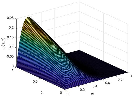
Figure 1. Three-dimensional solution profiles for Example 1.

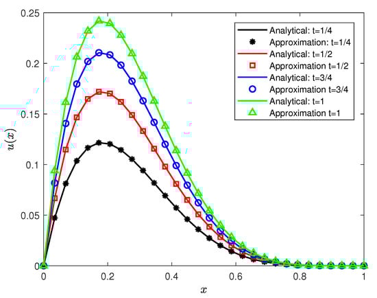
Figure 2. Comparison of the exact and numerical solutions for $u\left(\phi \right)$ at various time values for Example 1.

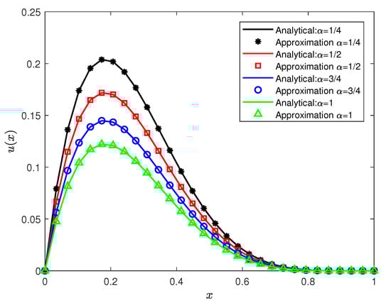
Figure 3. Effect of the fractional derivative ($\alpha$) on $u\left(\phi \right)$ for Example 1.

Table 1. Comparison of maximum errors: Conformable RNPSM with a high-order difference method for Example 1, where $M=100$ and $\alpha =0.4$.

$\mathit{\vartheta }$	RNPSM	High-Order Difference Method [26]
$0.25$	$2.1265\times {10}^{-07}$	$1.1873\times {10}^{-02}$
$0.125$	$1.2387\times {10}^{-08}$	$2.0365\times {10}^{-03}$
$0.0625$	$3.9521\times {10}^{-09}$	$4.7068\times {10}^{-04}$

Table 2. Comparison of error norms for Example 1 using the conformable RNPSM across various values of the fractional derivative ($\alpha$).

	$\mathit{\alpha }=0.5$		$\mathit{\alpha }=1.0$
$\mathbf{\vartheta }$	${\mathit{L}}_{\mathbf{\infty }}$	${\mathit{L}}_{\mathbf{2}}$	${\mathit{L}}_{\infty }$	${\mathit{L}}_{\mathbf{2}}$
$0.25$	$1.2322\times {10}^{-06}$	$1.7643\times {10}^{-07}$	$1.002\times {10}^{-06}$	$1.4398\times {10}^{-07}$
$0.5$	$2.2387\times {10}^{-06}$	$3.4531\times {10}^{-07}$	$2.1267\times {10}^{-06}$	$3.2365\times {10}^{-07}$
$0.75$	$4.6592\times {10}^{-06}$	$5.3212\times {10}^{-07}$	$4.3265\times {10}^{-06}$	$5.0936\times {10}^{-07}$
$1.0$	$6.7213\times {10}^{-06}$	$7.6555\times {10}^{-07}$	$6.1113\times {10}^{-06}$	$7.2012\times {10}^{-07}$

Example 2.

The following TFKdVB equation [29], where ${\sigma }_1=-6$, ${\sigma }_2=0$ and ${\sigma }_3=1$, is considered:

$$T_{\vartheta }^{\alpha }u-6u\left(\phi ,\vartheta \right){\displaystyle \frac{\partial u\left(\phi ,\vartheta \right)}{\partial \phi }}+{\displaystyle \frac{{\partial }^{3}u\left(\phi ,\vartheta \right)}{\partial {\phi }^3}}=0,0<\alpha \le 1,\phi \in [-10,10],\vartheta \in (0,1].$$

(32)

We have the following boundary and initial conditions:

$$\begin{array}{cc}\hfill & u\left(-10,\vartheta \right)=-{\displaystyle \frac{2e^{(-10-\vartheta )}}{1+e^{(-10-\vartheta )}}}\hfill \\ \hfill & u\left(10,\vartheta \right)=-{\displaystyle \frac{2e^{(10-\vartheta )}}{1+e^{(10-\vartheta )}}}\hfill \\ \hfill & u_{\phi }\left(10,\vartheta \right)={\displaystyle \frac{2e^{20-2\vartheta }}{{\left(1+e^{10-\vartheta }\right)}^2}}-{\displaystyle \frac{2e^{10-\vartheta }}{1+e^{10-\vartheta }}},\hfill \\ \hfill & u\left(\phi ,0\right)=-{\displaystyle \frac{2e^{\phi }}{1+e^{\phi }}},\hfill \end{array}$$

(33)

with the following exact solution

$$\begin{array}{c}\hfill u(\phi ,\vartheta )=-{\displaystyle \frac{2e^{(\phi -\vartheta )}}{1+e^{(\phi -\vartheta )}}}.\end{array}$$

(34)

In this section, the RPSM is employed to solve Example 2. The results demonstrate the effectiveness of RPSM in handling the fractional differential equation under study. Figure 4 provides a 3D surface plot of $u(\phi ,\vartheta )$ for Equation (32) with the initial conditions described in (33), where $\alpha =1.0$, $\phi \in [-10,10]$, and $\vartheta \in [0,1]$. The surface plot clearly shows the evolution of the solution over both spatial and temporal domains, giving insight into the behavior of $u(\phi ,\vartheta )$ as time progresses. Figure 5 presents a comparison between the exact solution of Example 2 and the RPSM solution at different time values. It can be observed that within the interval $\phi \in [-5,5]$ as time increases, the value of $u\left(\phi \right)$ also increases. Outside this range, the solution stabilizes and shows no significant change with respect to time, indicating a time-invariant behavior in these regions. Table 3 provides a quantitative comparison of norm errors between the exact solution and the RPSM solution. The results confirm that the present method is highly suitable for solving the TFKdVB equation. The RPSM shows good agreement with the exact solution, making it an accurate and reliable approach for this type of fractional differential equation. Overall, the conformable RPSM demonstrates excellent accuracy and stability in solving the TFKdVB equation, providing reliable solutions across both spatial and temporal domains.

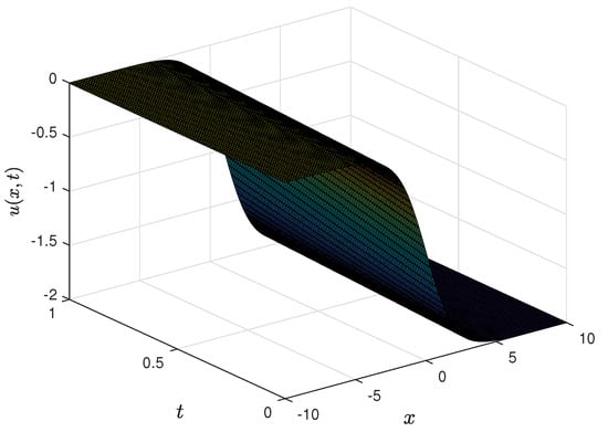
Figure 4. Three-dimensional solution profiles for Example 2.

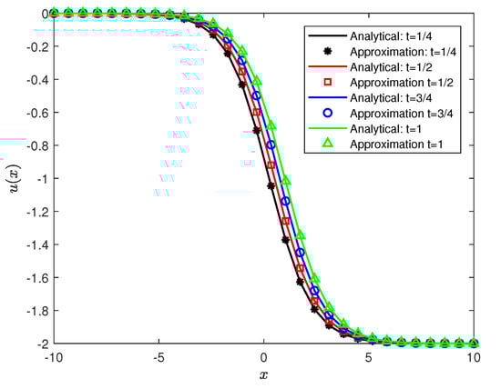
Figure 5. Comparison of the exact and numerical solutions for $u\left(\phi \right)$ at different time values in Example 2.

Table 3. Comparison of error norms for Example 2 using the conformable RNPSM where $\alpha =1$.

$\mathit{\vartheta }$	${\mathit{L}}_{\mathit{\infty }}$	${\mathit{L}}_2$
$0.25$	$2.3417\times {10}^{-07}$	$2.5411\times {10}^{-08}$
$0.5$	$3.6583\times {10}^{-07}$	$4.3376\times {10}^{-08}$
$0.75$	$5.6591\times {10}^{-07}$	$6.7980\times {10}^{-08}$
$1.0$	$7.6513\times {10}^{-07}$	$8.6042\times {10}^{-08}$

8. Conclusions

• The RNPSM was developed to solve the TFKdV equation, demonstrating both accuracy and efficiency.
• The method was applied to the time-fractional KdV–Burgers equation, showing conditional stability and a high convergence order.
• A comparison with the high-order difference method revealed that RNPSM offers superior accuracy, as confirmed by the norm error analysis.
• Results were presented in $2D$ and $3D$ formats, highlighting the robustness of the RNPS method.
• The effects of time and the fractional derivative were examined graphically, showcasing the method’s adaptability to a wide range of time-fractional problems.
• Overall, the RNPS method provides significant advantages over traditional numerical methods for solving TFDEs.

8.1. The Key Advantages of Using the RNPS Method

• Higher-order convergence: Ensures greater accuracy in numerical approximations.
• Ease of application: Simple implementation without complex computational requirements.
• Effective results: Delivers reliable and precise solutions for a wide range of problems.
• Adaptability: Well-suited for addressing the non-local and memory-dependent features of time-fractional differential equations.
• Improved stability: Demonstrates conditional stability verified through Fourier stability analysis.
• Versatility: Capable of handling various initial and boundary conditions effectively.
• Enhanced flexibility: Incorporates a rational function term, offering better adaptability than traditional polynomial-based methods.

8.2. The Limitations of the RNPS Method

The acknowledged limitations of the RNPS method include handling nonlinear terms in FDEs, solving high-degree FDEs, and addressing complex initial and boundary conditions. Future research could focus on refining the method to better accommodate these challenges, such as developing adaptive techniques or integrating hybrid approaches for enhanced versatility.

References

- Debnath, L. A brief historical introduction to fractional calculus. Int. J. Math. Educ. Sci. Technol. 2004, 35, 487–501. [Google Scholar] [CrossRef]
- Tepljakov, A. Fractional-Order Modeling and Control of Dynamic Systems; Springer: Berlin/Heidelberg, Germany, 2017. [Google Scholar]
- Chen, W.; Sun, H.; Li, X. Fractional Derivative Modeling in Mechanics and Engineering; Springer: Berlin/Heidelberg, Germany, 2022. [Google Scholar]
- Uchaikin, V.V. Fractional Derivatives for Physicists and Engineers: Volume I Background and Theory; Springer: Berlin/Heidelberg, Germany, 2013. [Google Scholar]
- Kulish, V.V.; Lage, J.L. Application of fractional calculus to fluid mechanics. ASME J. Fluids Eng. 2002, 124, 803–806. [Google Scholar] [CrossRef]
- Ionescu, C.; Lopes, A.; Copot, D.; Machado, J.A.T.; Bates, J.H.T. The role of fractional calculus in modeling biological phenomena: A review. Commun. Nonlinear Sci. Numer. Simul. 2017, 51, 141–159. [Google Scholar] [CrossRef]
- Agarwal, P.; Baleanu, D.; Chen, Y.; Momani, S.; Machado, T. Fractional Calculus; Springer: Berlin/Heidelberg, Germany, 2018. [Google Scholar]
- Vivas-Cortez, M.; Yousif, M.A.; Mohammed, P.O.; Lupas, A.A.; Ibrahim, I.S.; Chorfi, N. Hyperbolic non-polynomial spline approach for time-fractional coupled KdV equations: A computational investigation. Symmetry 2024, 16, 1610. [Google Scholar] [CrossRef]
- Vivas-Cortez, M.; Mohammed, P.O.; Guirao, J.L.G.; Yousif, M.A.; Ibrahim, I.S.; Chorfi, N. Improved fractional differences with kernels of delta Mittag–Leffler and exponential functions. Symmetry 2024, 16, 1562. [Google Scholar] [CrossRef]
- Khalil, R.; Al Horani, M.; Yousef, A.; Sababheh, M. A new definition of fractional derivative. J. Comput. Appl. Math. 2014, 264, 65–70. [Google Scholar] [CrossRef]
- Shi, L.; Tayebi, S.; Arqub, O.A.; Osman, M.S.; Agarwal, P.; Mahamoud, W.; Abdel-Aty, M.; Alhodaly, M. The novel cubic B-spline method for fractional Painlevé and Bagley-Trovik equations in the Caputo, Caputo-Fabrizio, and conformable fractional sense. Alex. Eng. J. 2023, 65, 413–426. [Google Scholar] [CrossRef]
- Yousif, M.A.; Hamasalh, F.K. The fractional non-polynomial spline method: Precision and modeling improvements. Math. Comput. Simul. 2024, 218, 512–525. [Google Scholar] [CrossRef]
- Vargas, A.M. Finite difference method for solving fractional differential equations at irregular meshes. Math. Comput. Simul. 2022, 193, 204–216. [Google Scholar] [CrossRef]
- Yang, Z.; Nie, Y.; Yuan, Z.; Wang, J. Finite element methods for fractional PDEs in three dimensions. Appl. Math. Lett. 2020, 100, 106041. [Google Scholar] [CrossRef]
- Ngo, H.T.B.; Razzaghi, M.; Vo, T.N. Fractional-order Chelyshkov wavelet method for solving variable-order fractional differential equations and an application in variable-order fractional relaxation system. Numer. Algorithms 2023, 92, 1571–1588. [Google Scholar] [CrossRef]
- Amin, M.; Abbas, M.; Iqbal, M.K.; Baleanu, D. Non-polynomial quintic spline for numerical solution of fourth-order time fractional partial differential equations. Adv. Differ. Equ. 2019, 2019, 183. [Google Scholar] [CrossRef]
- Khalid, N.; Abbas, M.; Iqbal, M.K.; Singh, J.; Ismail, A.I.M. A computational approach for solving time fractional differential equation via spline functions. Alex. Eng. J. 2020, 59, 3061–3078. [Google Scholar] [CrossRef]
- Li, M.; Ding, X.; Xu, Q. Non-polynomial spline method for the time-fractional nonlinear Schrödinger equation. Adv. Differ. Equ. 2018, 2018, 318. [Google Scholar] [CrossRef]
- Yousif, M.A.; Hamasalh, F.K. A hybrid non-polynomial spline method and conformable fractional continuity equation. Mathematics 2023, 11, 3799. [Google Scholar] [CrossRef]
- Hadhoud, A.R.; Srivastava, H.M.; Rageh, A.A.M. Non-polynomial B-spline and shifted Jacobi spectral collocation techniques to solve time-fractional nonlinear coupled Burgers’ equations numerically. Adv. Differ. Equ. 2021, 2021, 439. [Google Scholar] [CrossRef]
- Grad, H.; Hu, P.N. Unified shock profile in a plasma. Phys. Mech. 1967, 10, 2596–2601. [Google Scholar] [CrossRef]
- Jonson, R.S. Shallow water waves in a viscous fluid–the undular bore. Phys. Fluids 1972, 15, 1693–1699. [Google Scholar] [CrossRef]
- Jonson, R.S. A nonlinear equation incorporating damping and dispersion. J. Phys. Mech. 1970, 42, 49–60. [Google Scholar]
- Gupta, A.K.; Ray, S.S. On the solution of time-fractional KdV–Burgers equation using Petrov–Galerkin method for propagation of long wave in shallow water. Chaos Solitons Fractals 2018, 116, 376–380. [Google Scholar] [CrossRef]
- Ganie, A.H.; Mofarreh, F.; Khan, A. On new computations of the time-fractional nonlinear KdV-Burgers equation with exponential memory. Phys. Scr. 2024, 99, 045217. [Google Scholar] [CrossRef]
- Cen, D.; Wang, Z.; Mo, Y. Second order difference schemes for time-fractional KdV–Burgers’ equation with initial singularity. Appl. Math. Lett. 2021, 112, 106829. [Google Scholar] [CrossRef]
- Khan, A.; Akram, T.; Khan, A.; Ahmad, S.; Nonlaopon, K. Investigation of time fractional nonlinear KdV-Burgers equation under fractional operators with nonsingular kernels. AIMS Math. 2022, 8, 1251–1268. [Google Scholar] [CrossRef]
- Khader, M.M.; Saad, K.M.; Hammouch, Z.; Baleanu, D. A spectral collocation method for solving fractional KdV and KdV-Burgers equations with non-singular kernel derivatives. Appl. Numer. Math. 2021, 161, 137–146. [Google Scholar] [CrossRef]
- El-Ajou, A.; Al-Zhour, Z.; Oqielat, M.; Momani, S.; Hayat, T. Series solutions of nonlinear conformable fractional KdV-Burgers equation with some applications. Eur. Phys. J. Plus 2019, 134, 402. [Google Scholar] [CrossRef]
Disclaimer/Publisher’s Note: The statements, opinions and data contained in all publications are solely those of the individual author(s) and contributor(s) and not of MDPI and/or the editor(s). MDPI and/or the editor(s) disclaim responsibility for any injury to people or property resulting from any ideas, methods, instructions or products referred to in the content. |
© 2024 by the authors. Licensee MDPI, Basel, Switzerland. This article is an open access article distributed under the terms and conditions of the Creative Commons Attribution (CC BY) license (https://creativecommons.org/licenses/by/4.0/).