Prediction of Marine Shaft Centerline Trajectories Using Transformer-Based Models

Abstract

The accurate prediction of marine shaft centerline trajectories is essential for ensuring the operational performance and safety of ships. In this study, we propose a novel Transformer-based model to forecast the lateral and longitudinal displacements of ship main shafts. A key challenge in this prediction task is capturing both short-term fluctuations and long-term dependencies in shaft displacement data, which traditional models struggle to address. Our Transformer-based model integrates Bidirectional Splitting–Agg Attention and Sequence Progressive Split–Aggregation mechanisms to efficiently process bidirectional temporal dependencies, decompose seasonal and trend components, and handle the inherent symmetry of the shafting system. The symmetrical nature of the shafting system, with left and right shafts experiencing similar dynamic conditions, aligns with the bidirectional attention mechanism, enabling the model to better capture the symmetric relationships in displacement data. Experimental results demonstrate that the proposed model significantly outperforms traditional methods, such as Autoformer and Informer, in terms of prediction accuracy. Specifically, for 96 steps ahead, the mean absolute error (MAE) of our model is 0.232, compared to 0.235 for Autoformer and 0.264 for Informer, while the mean squared error (MSE) of our model is 0.209, compared to 0.242 for Autoformer and 0.286 for Informer. These results underscore the effectiveness of Transformer-based models in accurately predicting long-term marine shaft centerline trajectories, leveraging both temporal dependencies and structural symmetry, thus contributing to maritime monitoring and performance optimization.

1. Introduction

The prediction of ship main shaft centerline trajectories is a critical task in the maritime industry, as the alignment of the main shaft directly affects ship performance and safety [1,2]. Any misalignment in the main shaft can lead to significant mechanical problems, including increased wear, higher fuel consumption, and even potential failures in the propulsion system [3,4,5]. This, in turn, impacts the operational efficiency and reliability of the vessel, leading to higher maintenance costs and safety risks. The accurate prediction of the main shaft’s displacement and trajectory is essential for the early diagnosis of misalignments, which can prevent costly repairs and improve overall vessel performance [6,7].

Predicting the trajectory of the ship’s main shaft centerline is a complex challenge due to the dynamic nature of maritime environments. The main shaft is affected by a combination of internal mechanical factors and external forces such as sea states, currents, and vessel maneuvers [8]. These factors introduce long-term dependencies and non-linear behaviors in the displacement data, which are difficult to model accurately using traditional methods. Approaches such as autoregressive models and basic neural networks often struggle to capture both the short-term variations and the long-term trends in the data, resulting in decreased accuracy for extended predictions [9]. Transformer models have gained significant attention in recent years for their ability to handle sequential data, making them ideal candidates for predicting time series like the trajectory of a ship’s main shaft centerline [10,11,12,13,14,15,16,17]. Transformer architectures, particularly their self-attention mechanism, have been successfully applied in various time-series forecasting tasks, including energy consumption prediction, traffic flow forecasting, and mechanical system monitoring. These models excel at capturing long-range dependencies and dynamic patterns in sequential data, which are challenging for traditional methods like ARIMA and LSTM. However, standard Transformer models face significant challenges when applied to systems with inherent periodicity or symmetry, such as a ship’s shafting system. For instance, the self-attention mechanism struggles to efficiently capture cyclical patterns over long horizons, and the quadratic computational complexity of the attention mechanism can become prohibitive for large-scale time-series data. Furthermore, existing Transformer models are not inherently designed to leverage structural symmetries in data, such as the mirrored displacement patterns of left and right shafts in a marine propulsion system. These limitations highlight the need for architectural innovations to address these specific challenges in symmetry-aware time-series forecasting. One of the key strengths of Transformer architectures is their attention mechanism, which allows the model to focus on the most relevant parts of the input data sequence. This is especially useful for tasks that involve long-term dependencies, such as predicting shaft displacement over time. Unlike traditional models that struggle with sequential data or require large computational resources, Transformer models provide a more efficient and scalable solution for handling complex time series forecasting tasks.

While these advanced models have proven effective in capturing dynamic dependencies, another inherent feature of ships’ shafting systems is the structural symmetry between the left and right shafts. In most maritime vessels, the shafts operate under similar dynamic conditions and exhibit bilateral symmetry in their movements. This symmetry plays a significant role in the behavior of the shafting system, as both shafts typically experience similar forces and vibrations, which leads to synchronized displacements. From a modeling perspective, leveraging the symmetry of the shafting system presents an opportunity to enhance the predictive accuracy of Transformer-based models. The bilateral symmetry means that the displacement patterns of the left and right shafts are not only dynamically similar but also mirror each other. This mirror-like behavior implies that the displacement data for each side of the shaft are not entirely independent but exhibit certain spatial–temporal correlations. Recognizing and utilizing this symmetry can improve model efficiency by reducing the complexity of the input space and allowing the model to predict both forward and backward temporal dependencies more effectively. However, existing Transformer-based models lack the ability to explicitly encode such symmetry-aware relationships. Current approaches, such as Autoformer and Informer, focus primarily on improving efficiency through sparsity or auto-correlation mechanisms, but they do not address the unique challenges posed by systems with structural symmetries. Furthermore, these models often struggle to maintain accuracy over extended forecasting horizons, particularly in scenarios with significant periodic or mirrored displacement patterns. To bridge these gaps, our proposed BSAA and SPSA mechanisms extend the Transformer architecture to incorporate symmetry-aware learning and temporal decomposition. By explicitly modeling the spatial–temporal correlations and leveraging the bilateral symmetry of the shafting system, our approach offers a novel solution to long-term forecasting challenges in marine engineering systems.

Transformer models, with their ability to capture bidirectional dependencies, are particularly suited to account for mirrored displacement patterns. To address the limitations of standard Transformers in symmetry-aware systems, we propose two novel mechanisms: the Bidirectional Splitting–Agg Attention (BSAA) and the Sequence Progressive Split–Aggregation (SPSA). The BSAA mechanism extends the self-attention framework by splitting the input sequence into forward and backward temporal segments, enabling the model to learn bidirectional dependencies more effectively. This design is particularly suited for systems like ships’ shafting systems, where the bilateral symmetry of the left and right shafts results in mirrored displacement patterns. Mathematically, BSAA calculates separate attention weights for forward and backward sequences, which are then aggregated to enhance the model’s ability to capture spatial–temporal correlations. By doing so, BSAA directly leverages the structural symmetry inherent in the system, improving both prediction accuracy and computational efficiency. By incorporating Bidirectional Splitting–Agg Attention (BSAA) and Sequence Progressive Split–Aggregation (SPSA) mechanisms, we can enhance the model’s ability to capture both forward and backward temporal dependencies. The bidirectional attention mechanism mirrors the bilateral symmetry of the shaft system, thus enabling the model to consider both the past and future displacements of the shaft in a more balanced and synchronized manner. Furthermore, the symmetry of the shafting system can be encoded into the model by emphasizing spatial symmetry through the BSAA mechanism. This allows the model to better capture correlations between the displacement data of the left and right shafts, providing a more accurate and efficient prediction of their trajectories.

The primary objective of this research is to apply and modify Transformer-based models to accurately predict the lateral and longitudinal displacements of a ship’s main shaft, which define the shaft centerline trajectory. By introducing specific adjustments to the Transformer architecture—such as the Bidirectional Splitting–Agg Attention (BSAA) mechanism and the Sequence Progressive Split–Aggregation (SPSA) module—we aim to improve the model’s ability to capture the complex dependencies inherent in the displacement data. These modifications are designed not only to improve the model’s performance in handling long-term time-series data but also to exploit the inherent symmetry in the ship’s shaft system.

This research will demonstrate how these models can be effectively applied to predict long-term shaft centerline trajectories, offering a robust solution to a critical problem in the maritime industry.

2. Related Work

In this section, we present an overview of related work on ship main shaft trajectory prediction and time-series forecasting. First, we review traditional approaches, including Kalman filters, ARIMA, and classical neural network-based methods, highlighting their strengths and limitations. Next, we discuss the evolution of Transformer-based models and their applications in long-term forecasting tasks, particularly in handling complex temporal dependencies and long-range patterns. Finally, we introduce the key innovations of our proposed Transformer-based model and its ability to address the limitations of prior methods. This section sets the foundation for understanding the challenges in this domain and how our work builds upon and extends the current state of the art.

2.1. Traditional Approaches

Traditional methods for predicting ship main shaft centerline trajectories include Kalman filters [18], ARIMA models [19,20], and neural network-based approaches. Kalman filters are widely used for real-time state estimation in dynamic systems due to their efficiency in handling linear systems and measurement noise. However, their performance deteriorates in the face of non-linear dynamics typical of marine environments. Extensions like the Extended Kalman Filter (EKF) [21] and Unscented Kalman Filter (UKF) [22] attempt to mitigate these limitations by linearizing non-linear systems or applying statistical transformations, but they introduce computational complexity and still struggle with highly dynamic data. Similarly, ARIMA and its seasonal variant SARIMA [23] have been applied to time-series forecasting, effectively capturing short-term trends and periodic patterns. Despite this, ARIMA models are less effective in handling non-stationary data and long-term dependencies, which are critical in modeling shaft displacements influenced by changing sea conditions and mechanical vibrations.

It is essential to understand the structure and function of ships’ shafting systems, as illustrated in Figure 1. The shafting system is a critical component of a ship’s propulsion mechanism, linking the main propulsion motor to the propeller and ensuring efficient transmission of mechanical power [24]. This system comprises several interconnected elements, including the propeller, shaft bearings, thrust bearings, flexible coupling, intermediate bearings, and main shaft. The main shaft, in particular, plays a vital role in ensuring smooth power transmission and thrust generation. Any misalignment or deviation in the trajectory of the main shaft centerline, however minor, can cause excessive stress on the bearings, thrust bearing, and stern tube, leading to uneven wear, increased friction, and potential operational failures. The shafting system must continuously adapt to variable loads, changes in sea conditions, hull deformations, and vibrations caused by wave impacts and machinery operations. These factors introduce non-linear dynamics to the shaft movement, complicating the use of traditional linear models to capture the true behavior of the system. Deviations in the centerline of the shaft can also cause cavitation at the propeller, adversely affecting fuel efficiency and increasing the risk of mechanical failure.

Figure 1. Shafting system of a ship, illustrating key components involved in the power transmission from the main propulsion motor to the propeller.

In recent years, Convolutional Neural Networks (CNNs) [25] have emerged as powerful tools for time-series forecasting, particularly due to their ability to capture local patterns through convolutional operations. CNNs have been applied to mechanical systems and predictive maintenance tasks, such as predicting shaft trajectory and monitoring engine performance. With appropriate hyperparameter tuning, CNNs can achieve competitive accuracy. However, the primary limitation of CNNs lies in their inability to effectively capture long-term dependencies and sequential patterns, which are essential for tasks like ship main shaft trajectory prediction. While CNN-based models excel in detecting short-term patterns and anomalies, they struggle with tasks that require integrating both past and future dependencies over long periods. Recurrent Neural Networks (RNNs) [26,27,28,29,30,31], Long Short-Term Memory (LSTM) [32,33,34] networks, and LogTrans [35] networks have been employed to model sequence data for shaft trajectory prediction, offering the ability to capture both short-term fluctuations and long-term dependencies.

While LSTMs improve upon traditional RNNs by addressing the vanishing gradient problem, they require extensive computational resources and careful tuning to achieve optimal results in long-term prediction tasks. Other approaches, such as Support Vector Regression (SVR) [36], leverage kernel functions to handle non-linear relationships in displacement data, but their scalability and performance depend heavily on the selection of appropriate kernels. Frequency-based methods, such as Fourier analysis and wavelet transforms, are also used to identify periodic patterns in shaft movements but are less effective in modeling non-linear and stochastic behaviors. These limitations highlight the need for advanced models that can handle both the short-term and long-term complexities inherent in ship main shaft trajectory prediction, a gap that can be addressed by Transformer-based models.

2.2. Prediction Accuracy and Comparative Experiments

In recent years, Transformer-based models have gained significant attention for their ability to process time-series data, as seen in Figure 2, especially for long-term forecasting tasks. However, standard Transformer architectures face limitations when dealing with complex temporal dependencies and long-range patterns, primarily due to their quadratic computational complexity and inefficiency in handling extended sequences. Our work builds upon the strengths of the Transformer architecture and introduces several key modifications specifically designed to enhance its performance for predicting the trajectory of a ship’s main shaft centerline. We developed a novel model, which incorporates two significant innovations: the Bidirectional Splitting–Agg Attention (BSAA) mechanism and the Sequence Progressive Split–Aggregation (SPSA) module. These mechanisms were designed to address the challenges of capturing both forward and backward temporal dependencies and to improve the model’s ability to handle long-term time series data efficiently.

Figure 2. The architecture of time series forecasting based on Transformer models.

The BSAA mechanism enables the model to capture both forward and backward temporal dependencies simultaneously. By splitting the sequence into subcomponents and applying an attention mechanism bidirectionally, the model can more effectively learn from both past and future data points. This is crucial in accurately predicting the dynamic behavior of a ship’s main shaft, where both historical trends and future conditions influence trajectory. The BSAA also leverages Fourier transformation [37] to capture cyclical patterns within the data, enhancing the model’s ability to detect periodicities and long-range dependencies. The SPSA module was introduced to further improve the model’s ability to decompose time series data into trend and seasonal components. It progressively splits the input data into finer granularity and aggregates the information across different time scales. This not only reduces noise but also enhances the model’s ability to distinguish between short-term fluctuations and long-term trends, which is critical for accurately predicting the shaft centerline trajectory over extended periods. Empirical results from our experiments show that the SPSA module significantly boosts the model’s accuracy, particularly in scenarios involving long-term forecasting. The shafting system of a ship exhibits inherent bilateral symmetry, with left and right shafts operating under similar dynamic conditions. This structural symmetry provides a natural alignment with the bidirectional attention mechanism of the proposed Transformer-based model, allowing the model to leverage symmetric dependencies both in forward and backward directions. Such symmetry ensures a more accurate prediction of the axial displacements and enhances operational safety through precise long-term forecasting. In our comparative experiments, we demonstrated that our modified Transformer-based model, equipped with BSAA and SPSA, outperformed other state-of-the-art models such as Autoformer and Informer in terms of prediction accuracy and computational efficiency. The incorporation of these mechanisms led to a substantial reduction in Mean Squared Error (MSE) across multiple benchmark datasets, particularly for long-term predictions. Additionally, our visualization experiments, which mapped the predicted lateral and longitudinal displacements into a visual trajectory of the ship’s main shaft, showcased the practical applicability of our model in maritime operations. The model’s ability to handle complex temporal dependencies and efficiently predict the shaft centerline trajectory was clearly demonstrated through these visualizations.

2.3. Visualization of Shaft Centerline Trajectories

A critical component of our research involved not only improving the accuracy of ship main shaft centerline trajectory predictions but also providing comprehensive visualizations of these trajectories [38]. By plotting the predicted lateral and longitudinal displacement data, we generated detailed visual representations of the ship’s shaft movements, facilitating a direct comparison between predicted and actual trajectories.

These visualizations were instrumental in validating the Transformer-based model’s effectiveness. By transforming the displacement data into trajectory plots, we demonstrated how closely the model’s forecasts aligned with real-world shaft behavior. The visual comparisons highlighted both short-term fluctuations and long-term trends, showcasing the model’s ability to capture complex temporal dependencies and providing insights into its performance over extended periods. In our comparative studies, the accuracy of the Transformer-based model was benchmarked against traditional methods like ARIMA and LSTM, as well as more recent Transformer variants such as Informer and Autoformer. The visualized trajectories clearly indicated that our modified Transformer model consistently outperformed these alternatives, particularly in long-term forecasting, where other models struggled to maintain precision due to their limited capacity to capture long-range dependencies and non-linear dynamics. These visualizations also underscored the practical benefits of our model. By mapping predicted trajectories, we could easily identify periods of potential misalignment or mechanical stress on the shaft, offering valuable insights for real-time monitoring and predictive maintenance in maritime operations. This visualization approach improved both the interpretability and applicability of the model’s predictions, demonstrating its capacity to support advanced operational decision-making. In summary, the visualization of shaft centerline trajectories played a pivotal role in verifying the prediction accuracy of our model. It provided a clear and impactful method for comparing model outputs with actual data and highlighted the superior performance of our Transformer-based approach in capturing both short-term dynamics and long-term patterns in ship shaft trajectories.

In Table 1, To facilitate a clearer understanding of the symbols, abbreviations, and terminologies used throughout this study, a comprehensive Nomenclature and Symbols section is provided. This section aims to define all key mathematical symbols, technical terms, and abbreviations that appear in the subsequent chapters, particularly in the methodology and experimental analysis. By referring to this table, readers can efficiently interpret the equations, models, and concepts discussed in the paper. The Nomenclature and Symbols section is presented below before the detailed explanation of the proposed methodology.

Table 1. Nomenclature and symbols used in this study.

Symbol	Description	Unit
xd	Lateral displacement of the shaft centerline	mm
yd	Longitudinal displacement of the shaft centerline	mm
rd	Radial displacement	mm
ω	Rotational velocity of the shaft	RPM
T	Torque applied to the shaft	Nm
f	Frequency of the shaft’s oscillations	Hz
P	Power transmitted through the shaft	kW
δ	Angular displacement or misalignment	Degrees
Q	Query matrix used in the attention mechanism	-
K	Key matrix used in the attention mechanism	-
V	Value matrix used in the attention mechanism	-
ht	Hidden state vector at time t	-
xt	Input feature vector at time t	-
yt	Output prediction vector at time t	-
BSAA	Bidirectional Splitting–Agg Attention, a novel attention mechanism proposed in this study	-
SPSA	Sequence Progressive Split–Aggregation, a module designed to improve model efficiency and accuracy	-
MAE	Mean Absolute Error, a commonly used evaluation metric for time-series predictions	-
MSE	Mean Squared Error, another commonly used evaluation metric for time-series predictions	-
FFT	Fast Fourier Transform, used for frequency-domain analysis	-
ARIMA	Auto-Regressive Integrated Moving Average, a traditional time-series forecasting method	-
LSTM	Long Short-Term Memory, a type of recurrent neural network (RNN)	-
RNN	Recurrent Neural Network, commonly used for sequential data modeling	-
R2	Coefficient of Determination, a measure of the proportion of variance explained by the model	-

3. Methods

This study tackles the inherent complexities in predicting the trajectory of a ship’s main shaft centerline, specifically the challenge of accurately capturing both short-term fluctuations and long-term dependencies in displacement data. Traditional models often fall short in their ability to integrate both past and future dependencies in time series forecasting. To address these challenges, we propose an innovative approach that enhances model performance by employing sequence dimension splitting and aggregation mechanisms tailored to the dynamics of ship shaft trajectories. The development of the BSAA and SPSA mechanisms was inspired by advancements in attention mechanisms and time-series decomposition techniques. BSAA builds upon the foundation of the Transformer model’s self-attention mechanism introduced by Vaswani et al. [10], emphasizing bidirectional temporal processing to capture both past and future dependencies. This design was influenced by approaches such as Informer [11] and Autoformer [12], which highlighted the importance of efficient attention mechanisms for long-range time-series forecasting.

Additionally, the Fourier-based enhancements in BSAA are inspired by frequency-domain decomposition methods discussed in prior studies like Fedformer [16], which demonstrated the effectiveness of integrating spectral analysis to model cyclical patterns in data. On the other hand, the SPSA mechanism leverages concepts from multi-scale decomposition and aggregation as outlined in classical time-series techniques, including wavelet analysis [35], and recent innovations such as the auto-correlation approach in Autoformer [12]. These references collectively underscore the importance of combining temporal and frequency-domain insights to address the challenges of predicting complex marine shaft trajectories. By synergizing these methodologies, BSAA and SPSA ensure robust handling of both short-term fluctuations and long-term dependencies, thereby advancing the state of the art in Transformer-based time-series forecasting.

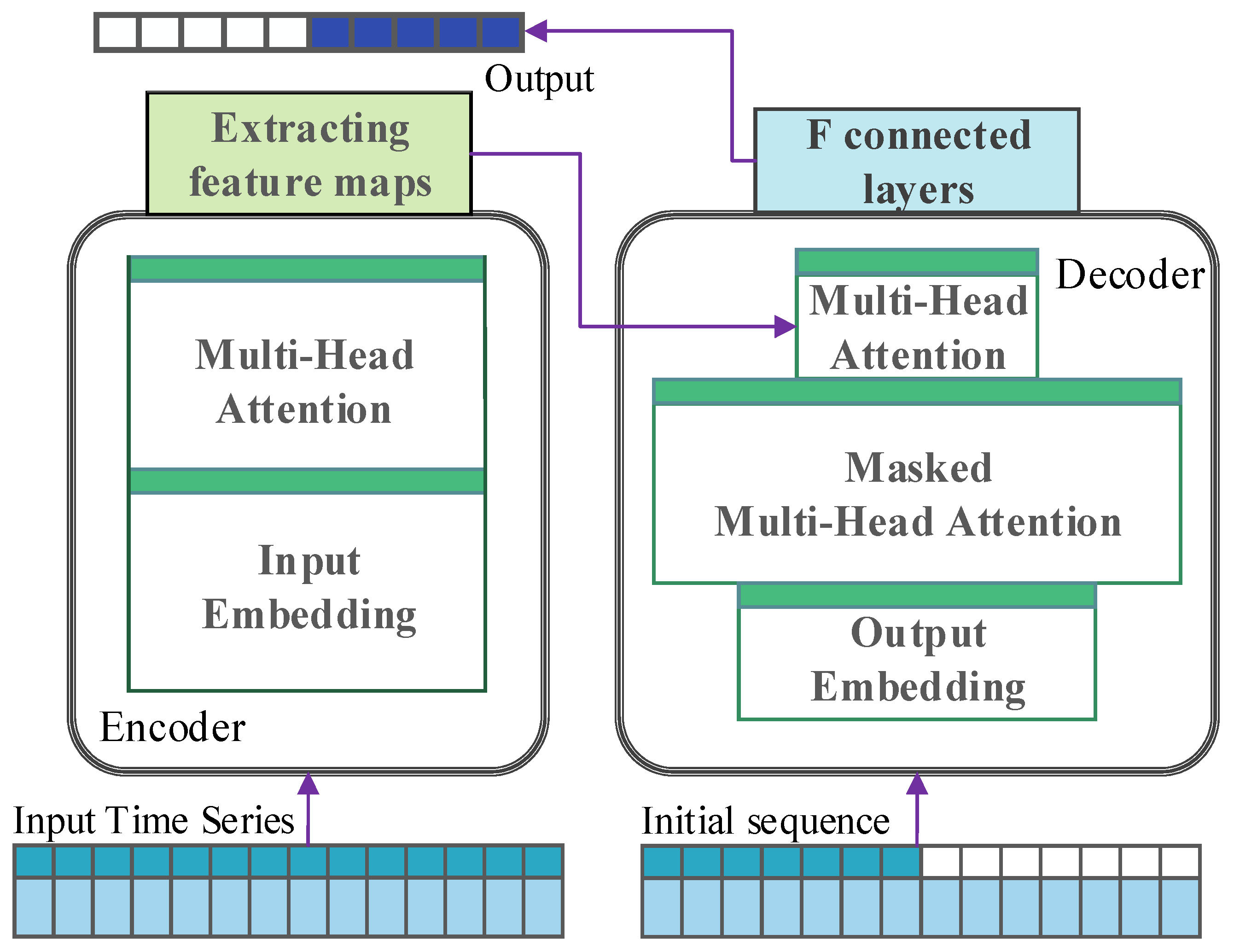
3.1. Model Architecture

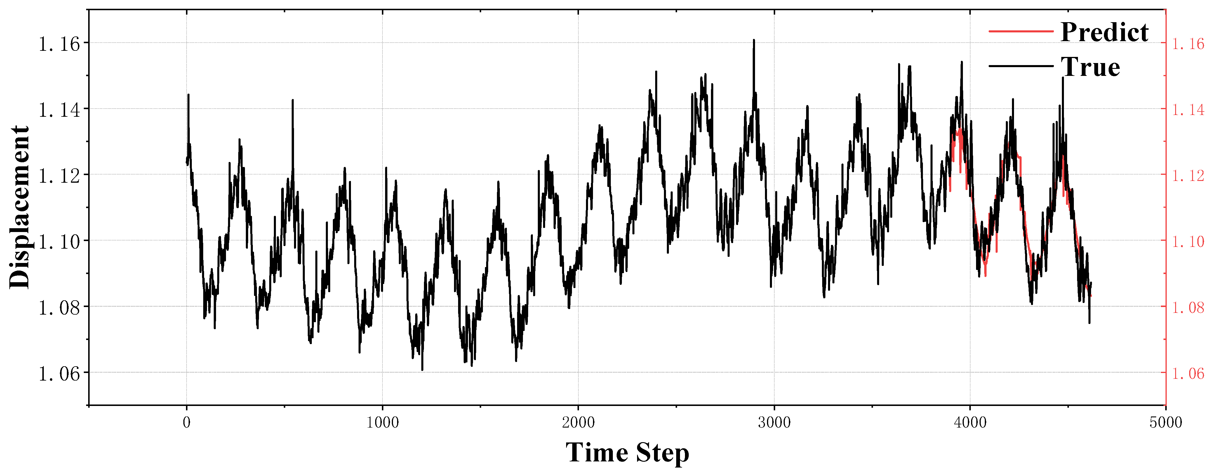
Accurately predicting ship main shaft centerline trajectories requires an effective approach to multivariate time-series forecasting, particularly in deciphering and leveraging critical signals to anticipate future trends. Each variable involved in the prediction process, such as lateral and longitudinal displacement, environmental conditions, and operational factors, plays a distinct role in shaping the trajectory forecast. A heatmap, shown in Figure 2, highlights the correlation patterns between each variable and the target forecast. These correlations are dynamic, shifting over time due to the complex interactions between mechanical and environmental factors. Capturing these temporal shifts is essential for enhancing the model’s predictive performance. Moreover, identifying and analyzing the interdependencies between these variables is crucial for improving prediction accuracy. The dynamic interplay between multiple variables adds depth to the analysis, enabling the model to better account for both short-term variations and long-term trends in the data. By incorporating these interdependencies into the proposed model, we significantly enhance its ability to produce more accurate and reliable forecasts. As detailed in the architectural diagram of the model (Figure 3), this study focuses on improving the model’s handling of complex temporal patterns, particularly those involving seasonal variations and trend-cyclical behaviors, to ensure robust long-term forecasting of the ship’s main shaft centerline trajectory. The key structural enhancements in this model are specifically designed to optimize its capacity for interpreting intricate temporal data in maritime applications.

Figure 3. Overall architecture diagram of BSAA algorithm model.

Figure 3 illustrates the architecture of the proposed BSAA algorithm model, highlighting the critical components and their roles in data processing. The workflow can be described in the following steps:

(1)

Input Embedding: The raw input time-series data (e.g., ship displacement signals) are first transformed into a high-dimensional feature space using an embedding layer. This step ensures the raw data are represented in a format suitable for downstream processing.

(2)

Encoder Processing:

(1)

Bidirectional Splitting–Agg Attention (BSAA): The encoder applies the BSAA mechanism to capture both past (backward attention) and future (forward attention) dependencies using a frequency-domain analysis.

(2)

Split Sequence and Convolution: The time-series data are then split into smaller temporal units and processed using sequential convolution operations. This step enhances feature extraction by isolating finer temporal components.

(3)

Feed-Forward Layer: Aggregates and refines the extracted features from the previous stages. These steps are repeated across multiple encoder blocks (N) to progressively improve the model’s ability to capture complex temporal patterns.

(3)

Decoder Initialization: The output of the encoder is split into two distinct components:

(1)

Seasonal Component: Captures periodic or cyclical patterns, such as vibrations or oscillations, in the ship’s shaft movement.

(2)

Trend Component: Represents long-term variations, such as changes in shaft displacement due to mechanical wear or external factors.

From a practical perspective, we consider the following:

Seasonal Component: Represents recurring mechanical patterns in the ship’s shaft system, such as vibrations induced by propulsion systems or regular operational maneuvers. For instance, during steady cruising, the propulsion shaft experiences consistent periodic oscillations, which are captured as seasonal variations.

Trend Component: Reflects long-term structural changes or operational shifts, such as gradual displacement caused by wear and tear in the mechanical system, or environmental factors like sea state and weather conditions.

(4)

Decoder Processing: The seasonal and trend components pass through separate BSAA mechanisms to further enhance their representations. Split Sequence and ADD Blocks are refined iteratively through multiple decoder layers (M), ensuring the precise modeling of both cyclical and long-term trends.

In the decoder, the seasonal component is passed through the BSAA mechanism to focus on high-frequency periodic patterns, effectively capturing the short-term cyclical variations critical for understanding mechanical vibrations. The trend component undergoes a smoothing and aggregation process through the BSAA mechanism to highlight long-term patterns and remove noise, ensuring the model captures gradual shifts caused by operational changes or environmental factors. By refining these two components separately and iteratively, the decoder achieves a precise balance between short-term responsiveness and long-term stability in its predictions.

(5)

Prediction Output: The refined seasonal and trend components are combined to generate the final prediction, which accurately captures both short-term fluctuations and long-term dependencies in the time-series data.

This modular architecture ensures the model is highly effective in modeling complex temporal patterns, enabling robust predictions of the ship’s main shaft trajectory. Each step in the workflow is carefully designed to optimize both computational efficiency and predictive accuracy, making the model suitable for real-world applications.

In the model architecture, the input to the encoder consists of the sequence $X_{\mathit{enc}}\in R^{I\times d}$, where $I$ denotes the time steps and $d$ represents the feature dimension. This sequence includes past time steps that encode historical data related to the ship’s displacement and other influencing factors. The input to the decoder, however, is split into two distinct components: the seasonal component $X_{\mathit{des}}$ and the trend-cyclical component $X_{\mathit{det}}$. These two components are extracted from the latter half of the encoder input and initialized using placeholders that account for both recent data and future trends. This process ensures that the model maintains sensitivity to recent information while providing a stable baseline for long-term forecasting. The mathematical representation of this process is as follows: Let the encoder input be $X_{\mathit{enc}}$. Then, the initialization process for the seasonal part $X_{\mathit{des}}$ and the trend-cyclical part $X_{\mathit{det}}$ of the decoder can be represented as

$$\begin{array}{c}{X}_{{\mathit{enc}}_{-}s}{,X}_{{\mathit{enc}}_{-}t}=\mathit{Split}(X_{\mathit{enc}}\left[\frac{I}{2}:I\right])\\ X_{\mathit{des}}=\mathit{Merge}(X_{{\mathit{enc}}_{-}s},Z_0)\\ X_{\mathit{det}}=\mathit{Merge}(X_{{\mathit{enc}}_{-}t},M_{\mathit{Xen}},)\end{array}$$

(1)

where $X_{{\mathit{enc}}_{-}s}{,X}_{{\mathit{enc}}_{-}t}\in R^{\frac{I}{2}\times d}$ represent the seasonal and trend-cyclical parts of $X_{\mathit{enc}}$, respectively; $Z_0{,M}_{\mathit{Xen}},\in R^{O\times d}$ represent placeholders filled with zeros and the mean of $X_{\mathit{enc}}$, respectively; and $O$ is the length of the placeholder. This design allows the model to be more responsive to recent data while also providing a more stable foundation for predicting future trends. By separating and processing the seasonal and trend-cyclical components in this manner, the architecture ensures that the model can efficiently handle the temporal variability inherent in ship main shaft trajectories.

Within the architecture, the encoder is tasked with modeling seasonal patterns in the data. The output of the encoder encapsulates past seasonal information, which is then utilized as cross-information to assist the decoder in refining prediction outcomes. This design is especially beneficial for capturing seasonal variations that frequently occur in time-series data related to ship movements, such as periodic fluctuations caused by mechanical vibrations or regular operational patterns. Summarizing the overall expression for the l-th layer of the encoder, let $X_{\mathit{enc}}^{(l)}$ be the output of the l-th layer, and $X_{\mathit{enc}}^{(l-1)}$ be the output of the (l-1)-th layer, as seen in the following formula:

$$X_{\mathit{enc}}^{(l)}=\mathit{EncLayer}(X_{\mathit{enc}}^{(l-1)})$$

(2)

This multi-layer design allows the model to progressively extract more complex temporal features as data move through each layer, improving the model’s ability to capture both short-term fluctuations and long-term trends in the ship main shaft’s trajectory. In the formula, EncLayer represents the operation of the encoder layer. For each layer of the encoder, its internal processing can be detailed as follows:

$$\begin{array}{c}{S}_{\mathit{enc}}^{(l,1)},\_=\mathit{SequenceSplitting}(\mathit{Bidirectional}-\mathit{Splitting}-\mathit{Agg}(X_{\mathit{enc}}^{(l-1)})+X_{\mathit{enc}}^{(l-1)})\\ S_{\mathit{enc}}^{(l,2)},\_=\mathit{SequenceSplitting}(FFN(S_{\mathit{enc}}^{(l,1)})+S_{\mathit{enc}}^{(l,1)})\end{array}$$

(3)

where Bidirectional-Splitting-Agg represents the BSAA mechanism, FFN refers to the Feed-Forward Neural Network, and Sequence Splitting corresponds to the Sequence Progressive Split–Agg operation. Specifically, $S_{\mathit{enc}}^{(l,i)}$ denotes the seasonal component of the l-th layer encoder after the i-th splitting block. The detailed implementation of the Bidirectional Splitting–Agg mechanism, which serves as a replacement for the traditional self-attention mechanism, will be described in the following section. This enhanced encoder architecture, which incorporates both frequency-domain Sequence Progressive Split–Agg operations and an advanced attention mechanism, empowers the model to more effectively capture and process seasonal variations in time-series data, specifically tailored to the dynamic behavior of ship shaft centerline displacement.

The decoder plays a critical role, comprising two key components: the accumulative structure for the trend-cyclical component and the enhanced BSAA mechanism designed for the seasonal component. Each decoder layer is constructed with both an improved internal BSA attention mechanism and the BSAA, facilitating communication between the encoder and decoder. This dual attention structure effectively refines predictions by leveraging historical seasonal data and extracting emerging trends and patterns from intermediate hidden variables. By focusing on cyclical dependencies, the decoder minimizes noise interference and hones in on crucial periodic trends. Structured in ’M’ layers, the decoder processes input from the encoder. For instance, considering a latent variable X1 received from the encoder, the operational dynamics of the l-th layer in the decoder can be articulated, focusing on the progressive refinement of trend predictions and the nuanced extraction of seasonal features. This layer-wise bidirectional approach allows the model to efficiently decompose and utilize complex time-series data, improving both prediction accuracy and the interpretability of forecasts. The process is mathematically expressed as

$$X_{\mathit{dec}}^{(l)}=DecLayer(X_{\mathit{dec}}^{(l-1)},X_{\mathit{enc}}^{(N)})$$

(4)

where DecLayer represents the operation of the decoder layer. The internal processing of each decoder layer can be described as

$$\begin{array}{c}{S}_{\mathit{dec}}^{(l,1)},T_{\mathit{dec}}^{(l,1)}=\mathit{SequenceSplitting}(\mathit{Bidirectional}-\mathit{Splitting}-\mathit{Agg}(X_{\mathit{dec}}^{(l-1)})+X_{\mathit{dec}}^{(l-1)})\\ S_{\mathit{dec}}^{(l,2)},T_{\mathit{dec}}^{(l,2)}=\mathit{SequenceSplitting}(\mathit{Bidirectional}-\mathit{Splitting}-\mathit{Agg}(S_{\mathit{dec}}^{(l,1)},X_{enc}^{(N)})+S_{\mathit{dec}}^{(l,1)})\\ S_{\mathit{dec}}^{(l,3)},T_{\mathit{dec}}^{(l,3)}=\mathit{SequenceSplitting}(FFN(S_{\mathit{dec}}^{(l,2)})+S_{\mathit{dec}}^{(l,2)})\end{array}$$

(5)

$$T_{\mathit{dec}}^{(l)}=T_{\mathit{dec}}^{(l-1)}+{\displaystyle \sum }_{i=1}^3{W}^{(l,i)}\cdot T_{\mathit{dec}}^{(l,i)}$$

(6)

where $T_{\mathit{dec}}^{(l)}$ is the trend-cyclical component accumulated by the l-th layer decoder; $S_{\mathit{dec}}^{(l,i)},T_{\mathit{dec}}^{(l,i)}$, respectively, represent the seasonal component and trend-cyclical component after the i-th splitting block of the l-th layer decoder; and $W^{(l,i)}$ is the projector of the i-th extracted trend $T_{\mathit{dec}}^{(l,i)}$. The final prediction result is the sum of these two split components, which can be represented as

$$FinalPrediction=W_S\cdot X_{\mathit{dec}}^{(M)}+T_{\mathit{dec}}^{(M)}$$

(7)

where $W_S$ is the weight matrix used to project the deeply transformed seasonal component $X_{\mathit{dec}}^{(M)}$ onto the target dimension. These enhancements allow the decoder to more effectively process both trend-cyclical and seasonal information, significantly improving the model’s accuracy in long-term time-series forecasting, particularly for predicting ship main shaft centerline trajectories.

To handle the complexities inherent in long-term forecasting, especially in maritime applications, the model adopts a Sequence Progressive Split–Agg strategy. This block progressively distills stable long-term trends from intermediate hidden variables, allowing for a more precise analysis of the time series. By mitigating cyclical noise through a moving average approach, the model highlights persistent trends, leading to improved projection accuracy and reliability in forecasting future sequences. For any given input sequence with length L, this splitting and smoothing operation can be mathematically delineated as

$${\tilde{\mathrm{X}}}_t=Smooth(\tilde{\mathrm{X}})=\tilde{\mathrm{X}}-{\tilde{\mathrm{X}}}_s$$

(8)

where ${\tilde{\mathrm{X}}}_t$ and ${\tilde{\mathrm{X}}}_s$ represent the trend-cyclical and seasonal parts, respectively, separated from the original sequence $\tilde{\mathrm{X}}$. This methodology enhances the predictive accuracy by isolating these components, thereby improving the model’s ability to capture and predict distinct patterns in the time series. A correlational pooling method is employed during the moving average process, and padding operations ensure that the sequence length remains unchanged. The bidirectional nature of the Splitting–Agg Attention mechanism introduces symmetry in the temporal processing of sequence data. By analyzing both past and future states, the model captures symmetrical patterns in the temporal structure, leading to more accurate and stable predictions, particularly for complex systems such as marine shafts that exhibit cyclic behavior over time.

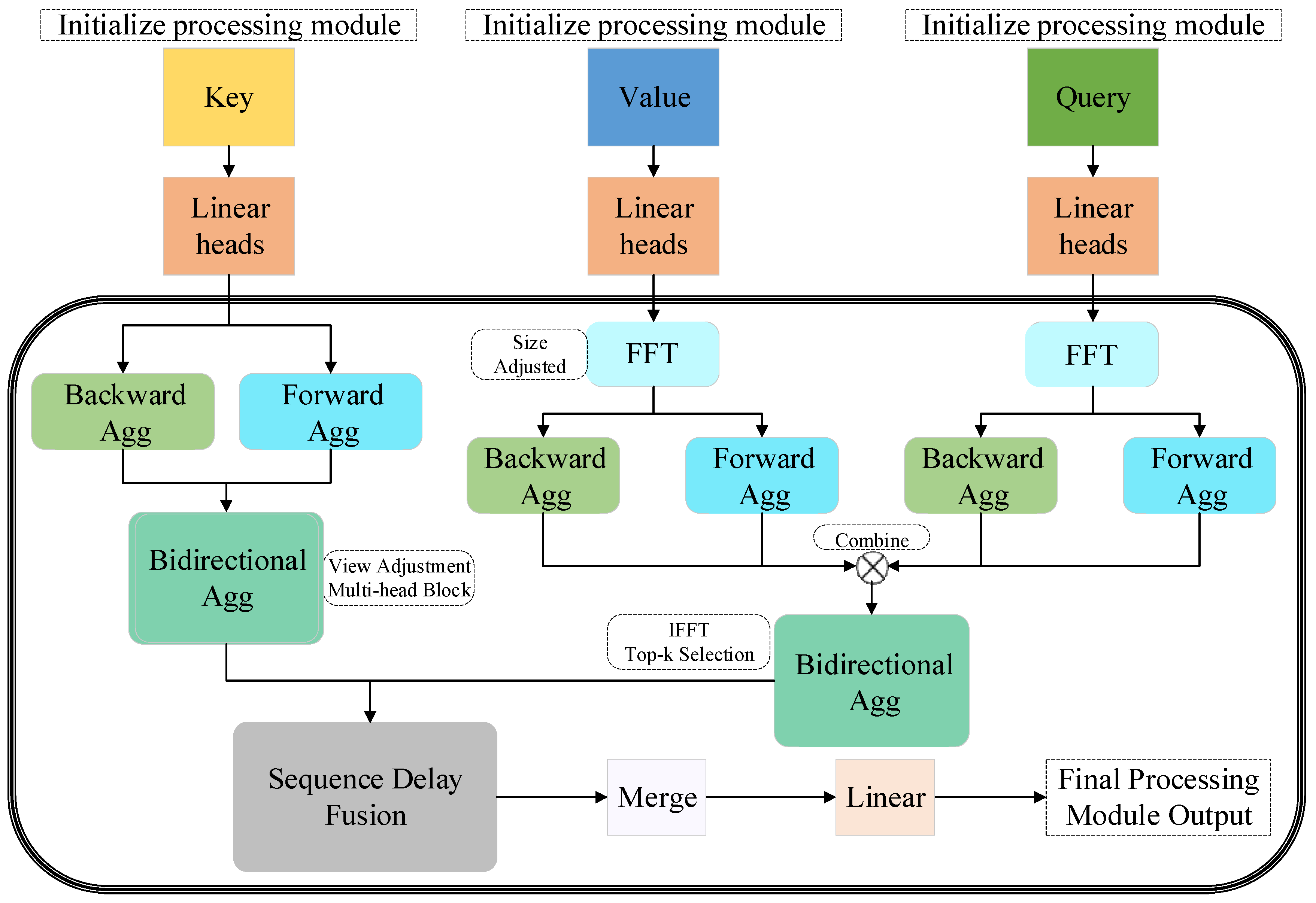
3.2. Bidirectional Splitting–Agg Attention Layer

This study advances time-series data analysis by introducing a BSAA layer, as shown in Figure 4. The BSAA layer enhances the model’s interpretative capability by processing both forward and backward temporal dependencies. This bidirectional mechanism is crucial for accurately predicting the trajectory of the ship’s main shaft, as it allows the model to capture complex cyclical and long-term dependencies inherent in the time-series data. By simultaneously calculating and aggregating attention across sub-sequences in both temporal directions, the model significantly improves its ability to understand and forecast the trajectory’s future behavior.

Figure 4. Bidirectional Splitting–Agg Attention mechanism diagram.

At the core of the BSAA layer are three distinct computational stages. The first stage involves calculating forward attention, achieved by applying a FFT to the query (Q) and value (V) components of the input time-series data. The FFT effectively transforms the data from the time domain into the frequency domain, enabling the model to detect periodic behaviors and cyclical patterns more efficiently. This frequency-domain processing is particularly suited for identifying long-term trends and seasonal variations within the ship’s shaft movement data. The computation for forward attention can be expressed as

$$\begin{array}{c}{Q}_{fft}^{forward}=FFT(Q_{permute})\\ V_{fft}^{forward}=FFT(V_{permute})\\ Cor{r}_{forward}=IFFT(Q_{fft}^{forward}\times V_{fft}^{forward})\end{array}$$

(9)

Here, $Q_{permute}$ and $V_{permute}$ are specifically arranged query and value matrices, adapted for FFT operations. $Cor{r}_{forward}$ represents forward correlation. In the proposed model, the initial step transitions time-series data from the time domain into the frequency domain using FFT. Following this transformation, the FFT results of both components are combined and subsequently reverted using an inverse FFT to delineate forward correlations, thereby unveiling the cyclical dependencies characteristic of the time series.

Following the forward attention computation, the model proceeds to calculate backward attention. This is achieved by reversing the sequence of the query and value components before applying FFT. This stage is essential for capturing temporal dependencies that flow from future states back to the past, a critical factor in modeling complex interactions in ship shaft trajectory data. The backward attention calculations are represented as follows:

$$\begin{array}{c}{Q}_{fft}^{backward}=FFT(flip{(Q)}_{permute})\\ V_{fft}^{backward}=FFT(flip{(V)}_{permute})\\ Cor{r}_{backward}=IFFT(Q_{fft}^{backward}\times V_{fft}^{backward})\end{array}$$

(10)

where $flip(Q)$ and $flip(V)$ represent the results of reversing the query and key matrices along the time axis, aiming to capture temporal dependencies from the future to the past, and $Cor{r}_{backward}$ is the forward–backward correlation. This process allows the model to discern backward temporal dependencies, effectively identifying future states that influence previous time steps, which is particularly important for long-term predictive accuracy in time-series forecasting.

Post these computations, the results derived from both forward and backward attention processes are synthesized. The fusion of these directional attentions is executed using a specific formula designed to amalgamate insights from both the past and the future of the series. The resultant aggregated output, denoted as R, is formulated as

$$R=w_f\cdot R_{forward}+w_b\cdot R_{forward}$$

(11)

where $w_f$ and $w_b$ are the weight coefficients for forward and backward attention, used to adjust the impact of attention in both directions on the final output. Through this BSAA mechanism, the model can more comprehensively capture the forward and backward dependencies in time series, thus providing a more accurate perspective for long-term time series prediction. By leveraging the BSAA mechanism, the model effectively captures the complex interactions between cyclical dependencies and long-term trends in ship shaft trajectory data. This approach enhances the model’s capacity for long-term forecasting by providing a more comprehensive understanding of the temporal structure, which is essential for accurate predictions of the ship’s main shaft centerline trajectory.

3.3. Exploration of Periodic Dependence and Aggregation Mechanism

Identifying these periodic dependencies is crucial for enhancing prediction accuracy, as ship operations often exhibit recurring patterns influenced by mechanical vibrations, operational conditions, and environmental factors. In Figure 5, building on the foundations of models such as Autoformer, this research refines the process of identifying and utilizing these cyclical variations through an advanced delayed split–aggregate analysis.

Figure 5. Sequence Progressive Split–Agg mechanism.

At the core of this approach is the calculation of the BSAA function, denoted as $B_{XX}^{\ast }(\delta )$, which provides a robust mechanism for recognizing and leveraging cyclical dependencies. This function captures the similarity between a sequence $\left\{X_t\right\}$ and itself over a lag $\delta$, identifying repeating patterns within the data that play a critical role in the trajectory prediction task. The correlation function is mathematically defined as

$$B_{XX}^{\ast }(\delta )=\underset{N\to \infty }{\lim }\frac{1}{N}{\displaystyle {\sum }_{t=1}^N((X_t\cdot X_{t-\delta })+ϵ)}$$

(12)

where $B_{XX}^{\ast }(\delta )$ captures the similarity of the sequence $\left\{X_t\right\}$ with its time series in an $\delta$-step delay. This BSAA function $B^{\ast }(\delta )$ is used as the basis for assessing the period length N. From a set of candidate period lengths, the k most likely period lengths ${\delta }_1\dots {\delta }_k$ are selected.

Using the insights gained from the periodic correlation function, this study further develops a method to balance forward and backward temporal dependencies through BSAA values across the selected period lengths. This mechanism allows the model to better discern and capture long-term cyclical dependencies that are often observed in ship shaft trajectory data, thus improving the accuracy of long-term forecasts. We enhanced the Time-Delayed Aggregation (TDA) mechanism, as illustrated in Figure 5. The Sequence Progressive Split–Agg Mechanism capitalizes on the temporal dependencies of the series, aligning and connecting subsequences within each cycle more effectively than traditional pointwise aggregations found in self-attention mechanisms. It determines the alignment of similar subsequences by leveraging selected parameters ${\delta }_1\dots {\delta }_k$, ensuring coherence within the estimated periods. Prior to aggregation, the importance of each subsequence is ascertained via an optimized SoftMax function, which takes into account not only the BSAA function values but also additional cyclical influences.

For the case of a single attention head, in the original time series, with the query Q, key K, and value V as preconditions, the time-delayed aggregation operation is defined as follows:

$$\begin{array}{c}{\delta }_1,\cdots ,{\delta }_k=\mathit{argTop}\left(B_{Q,K}\left(\delta \right)\right),\delta \in \left\{1,\dots \dots ,k\right\},k=\left[c\times \log L\right]\\ {\dot{B}}_{Q,K}({\delta }_1),\cdots ,{\dot{B}}_{Q,K}({\delta }_k)=\mathit{SoftMax}(B_{Q,K}({\delta }_1),\cdots ,B_{Q,K}({\delta }_k))\\ \mathit{Bidirectional}-\mathit{Splitting}-\mathit{Agg}(Q,K,V)={\displaystyle \sum _{i=1}^k}\mathit{For}-\mathit{Back}-\mathit{Agg}(V,{\delta }_i){\dot{B}}_{Q,K}({\delta }_i),\end{array}$$

(13)

Here, $B_{Q,K}\left(\delta \right)$ represents the BSAA function for query $Q$ and key $K$. As indicated by the mathematical expression, the function argTop(k) selects the top k values of the aggregate function, where c is a hyperparameter. The time-delayed aggregation mechanism includes aggregating the time series X forward and backward based on these parameters with the For-Back-Agg operation. In this operation, elements moved beyond the first position are reintroduced at the end of the series, where $K$ and $V$ are from the encoder $X_{\mathit{enc}}^{(N)}$, adjusted to length $O$, and $Q$ is from the previous block of the decoder.

To fully utilize the multi-head attention mechanism, a multi-head version is introduced to process hidden variables, which have $d_{\mathrm{model}}$ channels and are distributed across h different heads. For the $Q_i,K_i,V_i$ in the i-th head, the range is $Q_i,K_i,V_i\in R^{L\times \frac{d_{model}}{h}},i\in \left\{1,\cdots ,h\right\}$. This multi-head processing can be described as follows:

$$\begin{array}{c}\mathit{MultiHead}(Q,K,V)=W_{\mathit{output}}\times \mathit{Concat}({\mathit{head}}_1,\dots ,{\mathit{head}}_h)\\ {\mathit{head}}_i=\mathit{Bidirectional}-\mathit{Splitting}-\mathit{Agg}(Q_i,K_i,V_i)\end{array}$$

(14)

The above formulas use the FFT method for calculation. For the calculation of BSAA function values, given the time series $\left\{X_t\right\}$, $B_{XX}^{\ast }(\delta )$ is calculated using FFT. Let $A_{XX}(f)$ be the signal in the frequency domain; then, the calculation can be represented as

$$A_{XX}(f)=F(X_t)\cdot F^{*}(X_t)={{\displaystyle \int }}_{-\infty }^{\infty }{X}_t{e}^{-i2\pi tf}dt\overline{{{\displaystyle \int }}_{-\infty }^{\infty }{X}_t{\mathrm{e}}^{-i2\pi tf}dt}$$

(15)

where $F$ represents FFT, and $F^{*}$ is its conjugate operation. $B_{XX}(f)$ is in the frequency domain. Then, $B_{XX}^{\ast }(\delta )$ can be calculated through an inverse FFT operation:

$$B_{XX}^{\ast }(\delta )=F^{-1}(A_{XX}(f))={{\displaystyle \int }}_{-\infty }^{\infty }{A}_{XX}(f)e^{i2\pi f\delta }df$$

(16)

where $\delta \in \left\{1,\cdots \cdots ,L\right\}$ represents different time delays, and L is the length of the sequence. The model can quickly and accurately process long-term time-series data, especially when dealing with data characterized by significant cyclicity and seasonality. Through this method, the model’s performance is not only enhanced, but also the demand for computational resources is reduced, making the model more suitable for large-scale time-series forecasting tasks.

Our approach allows the model to efficiently process long-term time-series data, even in cases where significant periodicity and seasonality are present. By leveraging FFT and inverse FFT, the model can quickly detect and utilize periodic structures in the data, enhancing both its accuracy and computational efficiency. The ability to capture and process these long-term cyclical patterns makes the model particularly well suited for large-scale forecasting tasks such as predicting ship main shaft centerline trajectories.

3.4. Model Analysis

Within the proposed model framework, this study introduces a novel BSAA mechanism specifically designed to enhance the model’s capacity to capture both forward and backward temporal dependencies. Unlike traditional self-attention models, which primarily focus on current and past data, the BSAA mechanism offers a comprehensive, bidirectional analysis of time-series data. This approach is critical in accurately predicting the trajectory of the ship’s main shaft centerline, as it captures dynamic shifts and recurring cyclical patterns that may occur in both past and future time steps.

The BSAA mechanism operates by utilizing FFT in a bidirectional manner, transforming the input data into the frequency domain. By doing so, the model can detect and capitalize on key cyclical patterns and reverse temporal dependencies that are often difficult to discern using standard time-domain techniques. FFT allows the BSAA mechanism to efficiently handle complex frequency components within the displacement data, revealing long-term trends, periodic behaviors, and latent cyclical patterns that are critical for predicting ship shaft trajectories over extended periods. For instance, consider a univariate time-series input sequence $X=\left\{x_1, x_2, \dots , x_T\right\}$, representing the lateral displacement of a ship’s main shaft. The BSAA mechanism first splits the sequence into two sub-sequences: a forward sequence $X_f=\left\{x_1, x_2, \dots , x_T\right\}$ and a backward sequence $X_b=\left\{x_1, x_2, \dots , x_T\right\}$. The FFT is applied separately to each sequence, transforming them into the frequency domain as $\left\{FFT\right\}\left(X_f\right)$. This transformation captures periodic components and frequency-domain dependencies. The next step involves computing forward and backward attention weights using these transformed sequences. For example, forward attention identifies dependencies in $X_f$, such as the relationship between shaft displacements at $t_1$ and $t_{\mathrm{k}+1}$, where k denotes a periodic delay. Similarly, backward attention weights capture dependencies in $X_b$, such as the influence of future displacements on previous states. After computing forward and backward correlations, the results are combined using a weighted aggregation function:

$$R=\alpha \cdot FF{T}^{-1}(FFT(X_f))+\beta \cdot FF{T}^{-1}(FFT(X_b))$$

(17)

where $\alpha$ and $\beta$ are learned parameters that balance the contributions of forward and backward attention. This aggregated result $R$ represents the refined temporal dependencies that the model uses for downstream predictions. Through this process, the BSAA mechanism effectively identifies and integrates cyclical patterns, making it well suited for time-series data with pronounced periodicity, such as ship shaft trajectories.

The key strength of the BSAA mechanism lies in its ability to integrate insights from both forward and backward attention analyses. This bidirectional approach enables the model to develop a more complete understanding of the temporal structure within the data, leading to improved predictive precision. By leveraging forward attention, the model captures the historical influences on current shaft movements, while backward attention identifies potential future impacts on past behaviors, enabling more accurate and robust predictions.

Through the segmentation and aggregation of these temporal insights, the BSAA mechanism systematically identifies and capitalizes on periodic dependencies between subsequences. This segmentation process isolates important periodic features, allowing the model to focus on the most relevant temporal patterns. The segmentation of the input data into seasonal and trend-cyclical components has significant practical implications. The seasonal component helps identify consistent periodic behaviors, which are critical for monitoring routine mechanical vibrations and propulsion system operations. The trend-cyclical component, on the other hand, provides insights into long-term structural changes in the shaft system, such as those caused by wear and tear or environmental conditions. Together, these components provide a comprehensive understanding of the temporal dynamics, enabling the precise predictions of both recurring patterns and long-term shifts in the data. By incorporating these practical examples, we demonstrate how the BSAA and SPSA mechanisms operate in real-world scenarios, effectively capturing both short-term and long-term dependencies. This ensures that the proposed model is well equipped to address the challenges inherent in complex time-series forecasting tasks, such as predicting ship main shaft trajectories. The aggregation phase then combines these insights across different time periods, effectively aligning similar subsequences and improving the overall representation of the data. This method of segmenting and aggregating time-series data enables the model to handle long-term dependencies more effectively, providing a clearer view of how cyclic patterns influence future trajectories.

BSAA equips the model with a holistic understanding of sequence data by considering both preceding (forward attention) and subsequent (backward attention) elements. As depicted in Figure 4, this approach significantly augments the model’s contextual comprehension, thereby improving both the accuracy and efficiency of predictions. In the realm of time series analysis, it translates to an enhanced capability to discern and forecast patterns, including trends and seasonal variations. By assimilating forward and backward temporal relations, bidirectional attention substantially improves the model’s proficiency in recognizing cyclicality and trends, proving particularly beneficial in long-term forecasting and intricate seasonal pattern analysis.

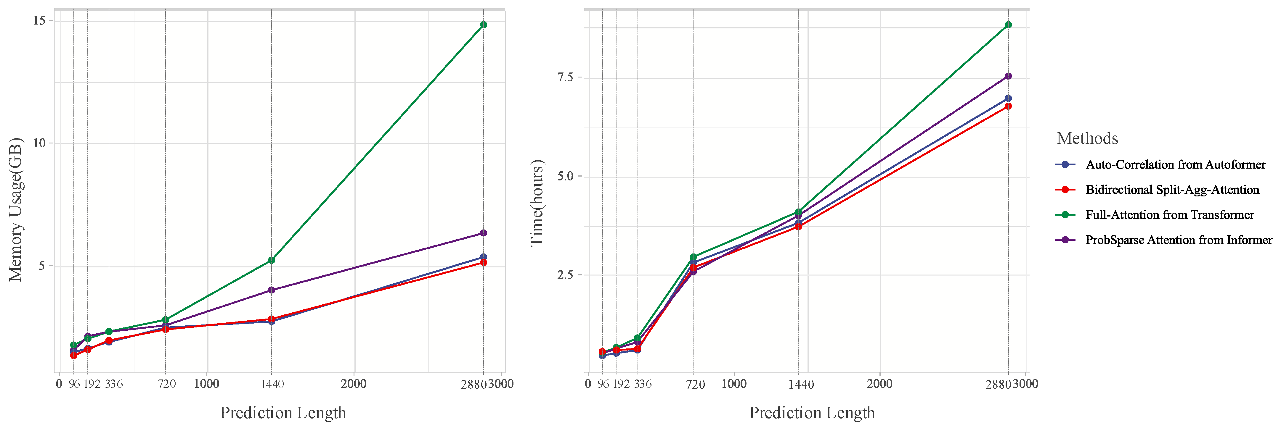
The BSAA and the SPSA module in this study notably reduce memory demands and enhance computational efficiency throughout the experimental process. Without compromising computational speed, they simultaneously refine the model’s ability to predict and delineate prominent growth trends and seasonal peaks.

Figure 6 presents a comparative analysis of memory usage and processing time across different models, including Autoformer, Informer, Transformer, and our proposed model, during the training phase. The results clearly highlight the computational efficiency of our approach:

Figure 6. Efficiency Analysis: For a fair comparison, we compared Informer, Autoformer, and Transformer models with the proposed Transformer-based model to verify its efficiency. On the ECL dataset, the output length exponentially increases with the input length of 96.

(1)

Memory Usage: For prediction lengths up to 720 steps, our model consumes 2.8 GB of memory, significantly lower than Transformer (4.2 GB) and comparable to Autoformer (2.7 GB) and Informer (2.9 GB). For longer prediction lengths (up to 3000 steps), our model maintains memory usage under 6 GB, while Transformer rises dramatically to 15 GB.

(2)

Processing Time: In terms of training time, our model demonstrates consistent improvements. For shorter prediction horizons (96 and 192 steps), the training time per epoch is 0.5 h, similar to Autoformer and Informer, and faster than Transformer. For longer prediction lengths (720 to 3000 steps), our model completes training within 5 h, compared to Transformer, which exceeds 7.5 h.

The identified time delay sizes indicate probable period lengths, aiding the model in employing the BSAA function for subsequences from corresponding or proximal stages. For the final time step, the BSAA adeptly employs analogous sequences, mitigating the shortcomings observed in self-attention models. This indicates that the model is capable of more completely and accurately capturing relevant information. Comparative assessments of operational memory and time during the training phase reveal that the BSAA-equipped Transformer-based model outshines its counterparts in both memory efficiency and long-term sequence handling, affirming its superior performance.

Table 2 presents a comparison of the time and space complexities of the models explored in this study, including the proposed Transformer-based model. Unlike the standard Transformer with $O(L^2\cdot d)$ time and $O(L^2)$ space complexity, our model achieves $O(L\log L)$ time complexity and $O(L\cdot d)$ space complexity. This improvement is due to the BSAA mechanism, which reduces computational load by processing sequences bidirectionally and leveraging Fourier transforms to capture periodic dependencies efficiently. While models such as Autoformer and Informer also achieve $O(L\log L)$ time complexity, they face specific limitations in handling complex and dynamic time-series data. Autoformer, for instance, relies on auto-correlation mechanisms that work well for stationary or quasi-stationary data but struggle with non-stationary patterns often observed in real-world datasets like ship shaft displacement. Similarly, Informer employs sparse attention to reduce computational overhead but sacrifices accuracy when dealing with sequences that exhibit intricate temporal dependencies or strong periodic components. In contrast, traditional models like LSTM and ARIMA, though effective for short-term or stationary datasets, are inherently constrained by scalability and their inability to model long-term, non-linear dynamics. For example, LSTM’s $O(L\cdot d^2)$ time complexity makes it computationally prohibitive for large-scale datasets, while ARIMA’s reliance on stationary assumptions limits its applicability to real-world scenarios with varying operational conditions. The proposed Transformer-based model overcomes these limitations by combining the BSAA and SPSA mechanisms, which are specifically designed to capture both bidirectional dependencies and complex periodic behaviors. This unique architecture ensures robustness and efficiency, making it better suited for real-world applications where long-term forecasting accuracy and computational scalability are critical.

Table 2. Comparison of time and space complexities across models.

Model	Time Complexity (T)	Space Complexity (S)	Explanation
Our Model	$O\left(L \log L\right)$	$O\left(L\cdot d\right)$	Incorporates the bidirectional splitting attention and frequency-domain aggregation for efficient long-term forecasting.
Autoformer	$O\left(L \log L\right)$	$O\left(L\cdot d\right)$	Reduces quadratic complexity via auto-correlation mechanism, but struggles with some sequence dependencies.
Informer	$O\left(L \log L\right)$	$O\left(L\cdot d\right)$	Introduces sparse attention to improve efficiency, yet limited for non-stationary data.
Transformer	$O\left(L^2\cdot d\right)$	$O\left(L^2\right)$	Suffers from quadratic complexity in long sequences.
LSTM	$O\left(L\cdot d^2\right)$	$O\left(L\cdot d+d^2\right)$	Effective in modeling dependencies but faces scalability issues in long-term predictions.
ARIMA	$O\left(L^2\right)$	$O\left(L\right)$	Limited to short-term stationary data, not effective for non-linear dynamics.

Compared to other Transformer variants like Autoformer and Informer, which offer O(LlogL) time complexity, the proposed model provides superior performance in scenarios with non-stationary and long-range dependencies. Traditional models like LSTM and ARIMA face challenges in handling such data effectively, either due to scalability issues or limitations with non-linear dynamics. The SPSA module in our model further optimizes memory usage by splitting and aggregating sequences progressively, ensuring the model remains both computationally efficient and accurate, particularly for long-term trajectory prediction in maritime applications.

The BSAA mechanism’s ability to sparsely represent and aggregate temporal data is a key contributor to the model’s superior accuracy and operational efficiency in long-term sequence forecasting. By integrating forward and backward temporal dependencies, and efficiently processing cyclical patterns, the BSAA mechanism empowers the model to provide highly accurate predictions of the ship’s main shaft centerline trajectory, even in challenging maritime environments characterized by complex temporal dynamics.

3.5. Implementation Framework for Model Construction and Training

To ensure the reproducibility of our model, we provide a comprehensive explanation of the primary components and configurations. The proposed Transformer-based model is designed to predict time-series data by leveraging our custom BSAA mechanism and SPSA module. These modules enable the model to capture both short-term fluctuations and long-term dependencies within the data, providing accurate predictions across multiple forecasting horizons.

The model begins with an embedding layer that converts the input time series into a high-dimensional space, capturing temporal features without relying on positional encoding. This design choice enables the model to process time-series data flexibly, focusing on content rather than position. The embedded data is then processed by the SPSA module, which performs seasonal and trend decomposition. This module decomposes the input sequence into seasonal and trend components through a custom moving average approach, helping the model isolate regular cyclic patterns from underlying trends. Implementing the SPSA module requires specifying parameters like the moving average window, which can be adjusted based on the dataset’s periodicity and trend characteristics. Within the encoder, the model uses the BSAA mechanism instead of the traditional self-attention mechanism. BSAA is designed specifically for time-series data, as it applies attention in both forward and backward directions, capturing temporal dependencies across multiple time scales. This bidirectional structure allows the model to understand dependencies from both past and future states, making it especially effective for complex time series with cyclical patterns. In the code, the BSAA module replaces conventional self-attention layers, with parameters tuned to optimize performance.

In the decoder, the model reconstructs the forecasted time series by combining outputs from the BSAA-encoded seasonal and trend components. The decoder utilizes cross-attention to align the seasonal and trend components, ensuring that short-term variations and long-term patterns are accurately represented in the final forecast. Additionally, the decoder incorporates the SPSA results, effectively merging short-term fluctuations with long-term trends to improve accuracy across different forecast horizons. During training, we employ the Adam optimizer with a learning rate scheduler, aiming for optimal convergence without overfitting.

4. Experiments

In this section, we evaluate the performance of our proposed model in predicting the trajectory of a ship’s main shaft centerline based on real-world displacement data. The real-world data include two key sources: publicly available datasets and confidential main shaft vibration datasets provided by our institutional collaborators. The publicly available datasets, such as ECL and Traffic, are widely used benchmarks for time-series forecasting tasks and are utilized in this study to validate the stability and generalizability of our model across various domains. For the main shaft vibration data, measurements were collected from real-world maritime environments through high-precision onboard sensors. These data capture the lateral and longitudinal displacements of the ship’s main shaft under actual operational conditions, reflecting both mechanical vibrations and external influences such as sea states and vessel maneuvers. We conducted comprehensive experiments to assess the model’s ability to capture both short-term and long-term dependencies in these complex time-series datasets. The effectiveness of the BSAA mechanism and the SPSA architecture is examined through comparisons with traditional and modern baseline models. The results highlight the robustness of our model in handling long-term forecasting challenges. The experimental setup, results, and visualizations are discussed in detail below.

4.1. Experimental Setup

All experiments in this study were computationally conducted using existing datasets. There is no physical experimental setup or laboratory apparatus involved. The computational experiments were designed to evaluate the performance of the proposed model using real-world data collected from ship operations and publicly available datasets.

4.1.1. Dataset

Our study began by evaluating the model on a variety of publicly available benchmark datasets across multiple sectors, including economics, energy, transportation, weather, and public health. This initial evaluation is crucial in demonstrating the model’s robustness and versatility across different real-world forecasting scenarios. The datasets used include the following:

(1)

ECL: Captures the hourly electricity consumption data of 321 customers over a span of two years, from 2012 to 2014. The dataset is accessible via https://archive.ics.uci.edu/dataset/321/electricityloaddiagrams20112014. Accessed on 23 March 2023.

(2)

ETT [11]: Consists of six characteristics of power load and oil temperature data in electricity transformers.

(3)

Traffic: Chronicles hourly changes in road occupancy rates via sensors on the San Francisco Bay Area highways. The dataset can be accessed at http://pems.dot.ca.gov. Accessed on 29 March 2023.

(4)

Weather: Features 21 meteorological indicators across nearly 1600 U.S. locations in 2022. Exchange: Tracks exchange rate data among eight countries from 1990 to 2016. The data are available through the Max Planck Institute for Biogeochemistry’s Weather portal at https://www.bgc-jena.mpg.de/wetter/. Accessed on 12 May 2023.

(5)

ILI: Compiles weekly influenza-like illness data from the U.S. CDC from 2002 to 2023. It is available at https://gis.cdc.gov/grasp/fluview/fluportaldashboard.html. Accessed on 24 May 2023.

All datasets were partitioned into training, validation, and test sets following standard protocols, with the ETT dataset using a 6:2:2 split and others a 7:1:2 ratio.

After validating the model on these publicly available datasets, we applied it to real-world ship main shaft displacement data to further test its effectiveness in a domain-specific context. The dataset used for this experiment comprises real-world measurements of ship main shaft displacements.

The data were collected using onboard sensors and include critical features such as rotational speed, power, axial x-displacement, axial y-displacement, and radial displacement. The main goal was to predict the future trajectory of the ship’s main shaft based on these measurements. The dataset has a sampling frequency of 51,200 Hz, ensuring high-resolution temporal data capture.

The data consist of 10 measurement tracks, each corresponding to different aspects of the shaft’s behavior, and a total of 900,608 data points, providing a robust basis for time-series forecasting. The dataset was divided into training, validation, and test sets following a 70:10:20 ratio to ensure fair model evaluation and validation. The key features of the dataset are as follows (Table 3).

Table 3. Key features of the ship main shaft displacement dataset, including displacement, velocity, and electrical parameters.

Track	Name	Unit	Description
Input 1	Axial x-displacement	mm	Axial displacement along the x-axis
Input 2	Axial y-displacement	mm	Axial displacement along the y-axis
Input 3	Radial displacement	mm	Radial displacement of the shaft
Input 4–6	Torsional velocity	RPM	Rotational speed in revolutions per minute
Ext. sync. 1	Voltage 1	V	Voltage potential difference
Ext. sync. 2	Voltage 2	V	Voltage potential difference

4.1.2. Baseline Methods

To evaluate the performance of our proposed model, we compared it against a comprehensive set of baseline models, including both traditional and advanced time-series forecasting approaches. The baseline models used in this study are as follows:

Informer [11]: A Transformer-based model optimized for long-term forecasting through sparse attention mechanisms, designed to reduce memory and computational costs.

Autoformer [12]: A Transformer-based model that enhances long-term time-series forecasting by leveraging auto-correlation mechanisms.

Pyraformer [13]: Another Transformer variant designed for improved efficiency and accuracy in handling long-sequence forecasting tasks.

Reformer [14]: A model that reduces the quadratic complexity of the original Transformer architecture, making it more suitable for large-scale time-series data.

LogTrans [35]: A logarithmic self-attention mechanism-based model, which improves the scalability and performance of Transformer models in time-series forecasting.

N-BEATS [39]: A deep learning model for time-series forecasting that focuses on trend and seasonal decomposition.

ARIMA [19]: A classical statistical model widely used for time-series prediction, particularly effective for short-term trends but limited in handling complex long-term dependencies.

LSTNet [34]: A neural network-based model that incorporates convolutional and recurrent layers to capture both short-term patterns and long-term dependencies in time-series data.

These models were trained and evaluated under the same conditions and with the same dataset splits, ensuring a fair comparison. The performance of each model was assessed using the same evaluation metrics to highlight the strengths of the proposed model in handling both short-term fluctuations and long-term dependencies in ship main shaft trajectory prediction.

4.1.3. Implementation Details

The proposed Transformer-based model was meticulously trained using a series of carefully designed strategies to ensure optimal performance. The model training utilized the L2 loss function with the Adam [40] optimizer, which is well suited for time-series forecasting tasks. The learning rate was initially set to 0.0001, and the batch size was chosen to be 32 to balance computational efficiency and memory usage during training.

To prevent overfitting, an early stopping strategy was applied, with training typically concluding after 10 epochs or earlier if no reduction in validation loss was observed for three consecutive epochs. All experiments were conducted on an NVIDIA RTX 3060 GPU, ensuring consistent and reliable computational performance across all models. The hyperparameter c, associated with the BSAA mechanism, was fine-tuned within the range of 1 to 2 to balance performance and computational efficiency. The model architecture comprises two encoder layers and one decoder layer, specifically designed to efficiently handle complex temporal dependencies in the input data.

Performance was evaluated using MSE (Mean Squared Error) and MAE (Mean Absolute Error) as the primary metrics, ensuring a comprehensive assessment of the model’s predictive accuracy. These metrics are defined as follows:

Mean Squared Error (MSE): Measures the average squared difference between the predicted and actual values. It is mathematically defined as

$$\mathit{MSE}={\displaystyle \frac{1}{n}}{\displaystyle \sum }_{i=1}^n{({\widehat{y}}_i-y_i)}^2$$

(18)

where ${\widehat{y}}_i$ represents the predicted value, $y_i$ represents the actual value, and n is the number of data points.

Mean Absolute Error (MAE): Measures the average absolute difference between the predicted and actual values. It is mathematically defined as

$$MAE={\displaystyle \frac{1}{n}}{\displaystyle \sum }_{i=1}^n|{\widehat{y}}_i-y_i|$$

(19)

Both metrics provide insights into the model’s predictive accuracy, with MSE assigning more weight to larger errors and MAE providing a more balanced view of overall error. All experiments were repeated five times to ensure the robustness of the results, with the average values across these repetitions forming the basis of the final analysis. The implementation of the model and the baseline models was carried out using the PyTorch [41] framework, known for its computational efficiency and flexible programming interface, making it ideal for handling large-scale time-series datasets and deep learning models.

4.2. Main Results

To ensure an equitable assessment across all models, we adopted uniform evaluation criteria for both the public datasets and the ship displacement data. The public datasets allowed us to validate the performance and versatility of the model across a wide range of real-world forecasting scenarios before applying it to the specific task of predicting the ship’s main shaft centerline trajectory.

The model was first evaluated on publicly available multivariate and univariate benchmark datasets. These experiments were crucial in verifying the model’s ability to generalize across different real-world domains such as energy, transportation, weather, economics, and public health.

Table 4 presents the results of the multivariate time-series forecasting for datasets such as ECL, Traffic, and ETT. Table 5 provides the results for univariate forecasting using datasets such as ETTm2 and Exchange. The performance is evaluated based on MSE across different forecast lengths. The table presents the experimental results for multivariate and univariate public datasets, respectively, comparing the performance of multiple state-of-the-art models, including our model, Autoformer, Informer, Pyraformer, Reformer, N-BEATS, ARIMA, and LogTrans. The metrics forecast horizons set at 96, 192, 336, and 720 steps. The bold font is used to represent the optimal experimental results.

Table 4. Multivariate public dataset results comparing MSE and MAE across various models.

Model		Our Model		Autoformer		Informer		Pyraformer		Reformer		LogTrans		LSTNet
Metric		MSE	MAE	MSE	MAE	MSE	MAE	MSE	MAE	MSE	MAE	MSE	MAE	MSE	MAE
ECL	96	0.192	0.300	0.201	0.317	0.274	0.368	0.386	0.449	0.986	0.779	0.840	0.677	1.100	0.806
	192	0.209	0.326	0.222	0.334	0.296	0.386	0.378	0.443	1.011	0.783	0.916	0.689	1.096	0.804
	336	0.223	0.335	0.231	0.338	0.300	0.394	0.376	0.443	1.088	0.786	0.981	0.772	1.103	0.805
	720	0.254	0.347	0.254	0.361	0.373	0.439	0.376	0.445	1.062	0.791	1.032	0.804	1.113	0.808
Traffic	96	0.579	0.362	0.613	0.388	0.719	0.391	0.684	0.393	0.732	0.423	0.684	0.384	1.107	0.685
	192	0.582	0.357	0.616	0.382	0.696	0.379	0.692	0.394	0.733	0.420	0.685	0.390	1.157	0.706
	336	0.588	0.361	0.622	0.337	0.777	0.420	0.699	0.396	0.742	0.420	0.733	0.408	1.216	0.730
	720	0.621	0.385	0.660	0.408	0.864	0.472	0.712	0.404	0.755	0.423	0.717	0.396	1.481	0.805
ETTm1	96	0.442	0.432	0.523	0.488	0.615	0.556	0.536	0.506	0.778	0.623	0.588	0.593	2.003	1.218
	192	0.487	0.461	0.543	0.498	0.723	0.620	0.539	0.520	0.929	0.707	0.769	0.793	2.764	1.544
	336	0.513	0.502	0.675	0.551	1.300	0.908	0.720	0.635	1.016	0.733	1.462	1.320	1.257	2.076
	720	0.521	0.518	0.683	0.573	0.972	0.744	0.940	0.740	1.122	0.793	1.669	1.461	1.917	2.941
ETTh1	96	0.502	0.518	0.536	0.548	0.984	0.786	0.783	0.657	0.773	0.640	0.767	0.758	1.457	0.961
	192	0.537	0.524	0.543	0.551	1.027	0.791	0.863	0.709	0.910	0.704	1.003	0.849	1.998	1.215
	336	0.543	0.537	0.615	0.592	1.032	0.774	0.941	0.753	1.000	0.760	1.362	0.952	2.655	1.369
	720	0.538	0.549	0.599	0.600	1.169	0.858	1.042	0.819	1.242	0.860	1.397	1.291	2.143	1.380

Table 5. Univariate public dataset results comparing MSE and MAE across various models.

Model		Our Model		Autoformer		Informer		Pyraformer		Reformer		N-BEATS		ARIMA		LogTrans
Metric		MSE	MAE	MSE	MAE	MSE	MAE	MSE	MAE	MSE	MAE	MSE	MAE	MSE	MAE	MSE	MAE
Exchange	96	0.226	0.348	0.241	0.387	0.591	0.615	0.290	0.439	1.327	0.944	0.247	0.312	0.112	0.245	0.237	0.377
	192	0.248	0.371	0.273	0.403	1.183	0.912	0.594	0.644	1.258	0.924	0.652	0.613	0.304	0.404	0.738	0.619
	336	0.473	0.519	0.508	0.539	1.367	0.984	0.962	0.824	2.179	1.296	0.611	0.605	0.736	0.598	2.018	1.070
	720	0.853	0.724	0.991	0.768	1.872	1.072	1.285	0.958	1.280	0.953	1.111	0.860	1.871	0.935	2.405	1.175
ETTm2	96	0.068	0.192	0.065	0.189	0.088	0.225	0.074	0.208	0.131	0.288	0.082	0.219	0.211	0.362	0.125	0.238
	192	0.103	0.228	0.118	0.256	0.132	0.283	0.116	0.252	0.186	0.354	0.120	0.268	0.261	0.406	0.179	0.295
	336	0.145	0.289	0.154	0.305	0.180	0.336	0.143	0.295	0.220	0.381	0.226	0.370	0.317	0.448	0.201	0.332
	720	0.186	0.331	0.182	0.335	0.300	0.435	0.197	0.338	0.267	0.430	0.188	0.338	0.366	0.487	0.248	0.389

All these results demonstrate that the proposed model consistently outperforms other models, particularly in long-term prediction tasks, where capturing forward and backward temporal dependencies is critical. This performance validates the robustness of the BSAA mechanism. Figure 7a and Figure 8a show our model, Figure 7b and Figure 8b show Informer, and Figure 7c and Figure 8c show Autoformer. The blue line represents the ground truth and the orange line represents the prediction. The proposed model consistently outperforms other models, particularly in long-term prediction tasks, where capturing forward and backward temporal dependencies is critical. This performance validates the robustness of the BSAA mechanism. The blue line in Figure 7 and Figure 8 represents the ground truth, which corresponds to the actual observed values of the target variable in the respective datasets. Specifically, for Figure 7, the ground truth is derived from the ETTm2 dataset, which includes real-world electricity and oil temperature data over a prediction horizon of 196 time steps. In Figure 8, the ground truth comes from the ETTm1 dataset, representing observed values over a longer prediction horizon of 720 time steps. These ground-truth values are sourced from widely recognized and publicly available datasets, which were preprocessed and validated by their authors to ensure accuracy and reliability. These datasets are commonly used in time-series forecasting research for benchmarking purposes and provide a trusted reference for evaluating model predictions. The orange line in the figures denotes the predictions generated by the respective models. The close alignment between the blue and orange lines in Figure 7a and Figure 8a highlights the superior ability of our proposed model to accurately capture both short-term variations and long-term trends. In contrast, the predictions generated by the baseline models, such as Informer (Figure 7b and Figure 8b) and Autoformer (Figure 7c and Figure 8c), demonstrate larger deviations from the ground truth, particularly in scenarios requiring long-term forecasting. By comparing the predicted values (orange line) with the ground truth (blue line), we validate the effectiveness of the BSAA mechanism and the overall architecture of our proposed model. This comparison further emphasizes the robustness and accuracy of our approach in handling complex time-series forecasting tasks.

Figure 7. Visualizes the predictions for the ETTm2 dataset across different models over 196 time steps. The horizontal axis represents the prediction time steps, while the vertical axis denotes the predicted value of the target variable., where image (a) represents the complete our model, image (b) represents our model without the SPSA mechanism, and image (c) represents the Autoformer [12] model.

Figure 8. Visualizations of univariate predictions on the ETTm1 dataset across different models over 720 time steps, where image (a) represents the complete model, image (b) represents the model without the SPSA mechanism, and image (c) represents the Autoformer [12] model.

After validating the proposed model on the public datasets, we adopted uniform evaluation criteria for each baseline and the proposed model. Specifically, the historical sequence length for the dataset was standardized at 96 steps for both the axial x-displacement and axial y-displacement data. The forecast lengths used for comparison were {96, 192, 336, 720} steps, which provided a comprehensive evaluation of the models’ ability to capture both short-term and long-term dependencies in the time-series data.

The results, presented in Table 6 and Table 7, highlight the robustness and superior performance of the proposed model across both displacement dimensions. Table 6 focuses on the axial x-displacement prediction results, while Table 7 provides the same for the axial y-displacement predictions. The proposed Transformer-based model demonstrates significant improvements over other models in terms of both MSE and MAE, particularly in long-term forecasting tasks (336 and 720 steps). In addition to MSE and MAE, we included the $R^2$ metric in both tables to provide a more comprehensive evaluation of model performance. The $R^2$ metric quantifies the proportion of variance in the ground truth explained by the predictions, with values closer to 1 indicating better alignment. Across all datasets and prediction horizons, our model consistently achieves higher $R^2$ values than baseline models, further underscoring its ability to accurately capture both short-term fluctuations and long-term dependencies. This enhancement allows for a more intuitive understanding of the model’s predictive capabilities and its superiority in time-series forecasting tasks. The bold font is used to represent the optimal experimental results.

Table 6. Axial x-displacement prediction results.

Model\Steps	96 Steps	96 Steps	96 Steps	192 Steps	192 Steps	192 Steps	336 Steps	336 Steps	336 Steps	720 Steps	720 Steps	720 Steps
MAE/MSE/R2	MAE	MSE	R2	MAE	MSE	R2	MAE	MSE	R2	MAE	MSE	R2
Our Model	0.232	0.209	0.954	0.263	0.284	0.948	0.212	0.249	0.96	0.239	0.335	0.935
Autoformer	0.235	0.242	0.951	0.231	0.298	0.944	0.221	0.234	0.959	0.245	0.339	0.93
Informer	0.264	0.286	0.935	0.376	0.385	0.92	0.275	0.297	0.94	0.326	0.397	0.91
Pyraformer	0.376	0.368	0.89	0.376	0.376	0.89	0.387	0.379	0.91	0.371	0.448	0.89
Reformer	0.489	0.433	0.85	1.188	1.262	0.74	0.439	0.463	0.83	1.082	1.138	0.72
LogTrans	0.890	0.926	0.78	0.991	1.132	0.72	0.893	0.926	0.78	0.941	0.985	0.74
LSTNet	1.133	1.291	0.71	1.123	1.243	0.69	1.174	1.086	0.7	1.008	1.176	0.7

Table 7. Axial y-displacement prediction results.

Model\Steps	96 Steps	96 Steps	96 Steps	192 Steps	192 Steps	192 Steps	336 Steps	336 Steps	336 Steps	720 Steps	720 Steps	720 Steps
MAE/MSE/R2	MAE	MSE	R2	MAE	MSE	R2	MAE	MSE	R2	MAE	MSE	R2
Our Model	0.238	0.220	0.956	0.255	0.297	0.948	0.235	0.348	0.94	0.262	0.355	0.935
Autoformer	0.248	0.320	0.95	0.258	0.319	0.945	0.237	0.352	0.938	0.263	0.364	0.93
Informer	0.261	0.362	0.94	0.355	0.397	0.92	0.314	0.441	0.91	0.384	0.442	0.9
Pyraformer	0.331	0.435	0.91	0.383	0.454	0.89	0.389	0.455	0.89	0.387	0.459	0.88
Reformer	0.485	1.692	0.73	0.440	1.058	0.75	1.123	1.146	0.71	1.076	1.079	0.74
LogTrans	0.869	0.911	0.78	0.810	0.937	0.74	0.826	0.919	0.75	1.243	1.369	0.72
LSTNet	1.183	1.207	0.72	1.029	1.194	0.69	1.123	1.298	0.7	1.045	1.291	0.69

The following figures, Figure 9 and Figure 10, illustrate the prediction performance of our model for axial x-displacement and y-displacement over 720 time steps. As shown, the predicted vibration trends align closely with the actual displacement values, demonstrating the model’s capability to capture both short-term fluctuations and long-term trends with high precision. The predicted curves follow the actual trajectories, confirming the effectiveness of our approach in handling complex dynamic behavior in the ship’s main shaft system.

Figure 9. Prediction of axial x-displacement over 720 time steps.

Figure 10. Prediction of axial y-displacement over 720 time steps.

Our model demonstrates an impressive reduction in MSE and MAE compared to the baseline models, particularly in long-term forecasts, where it captures both forward and backward temporal dependencies effectively. This is especially evident in the 336- and 720-step prediction horizons, where the proposed model consistently outperforms the other models. Across both axial x-displacement and y-displacement datasets, our approach showcases its strength in handling long-term forecasting tasks, thus demonstrating its adaptability to complex, multivariate time-series data in real-world maritime environments.

4.3. Visualization

In this section, we present the visualization of the predicted ship shaft centerline trajectory over 720 time steps. These visualizations are crucial for understanding the model’s ability to capture the intricate patterns of the shaft’s axial motion. The shaft centerline trajectory is visualized as circular motion, where both the real and predicted paths are compared. Each figure contains a horizontal and vertical reference line to mark the shaft centerline’s position, with the blue line representing the actual measured trajectory, and the red and orange lines representing the predicted trajectories.

These visualizations illustrate the axial x-displacement (horizontal axis) and y-displacement (vertical axis) of the shaft centerline. The predicted trajectories were generated using the proposed Transformer-based model over 720 time steps. The real shaft centerline movement, captured by onboard sensors, is shown in blue, while the predicted trajectories are represented by red and orange lines.

The four visualizations provide a comprehensive overview of the model’s predictive capability across different operational conditions. In both the 200 RPM and 250 RPM scenarios, the predictions closely follow the real centerline trajectories, demonstrating the model’s effectiveness in capturing complex shaft motions. In Figure 11a,b, which depict the left and right shaft movements at 200 RPM, the predicted trajectories (red or orange) align well with the actual trajectory (blue). The model successfully tracks the cyclic movement of the shaft’s centerline, accurately capturing both the short-term variations and long-term patterns in the motion.

Figure 11. Shaft centerline trajectory prediction over 720 time steps under different rotational speeds. (a): Predicted and actual trajectory of the left shaft at 200 RPM. (b): Predicted and actual trajectory of the right shaft at 200 RPM. (c): Predicted and actual trajectory of the left shaft at 250 RPM. (d): Predicted and actual trajectory of the right shaft at 250 RPM.

Similarly, Figure 11c,d show the model’s predictions at 250 RPM for the left and right shafts, respectively. Despite the increase in rotational speed, the predicted trajectories maintain high fidelity to the real shaft movement. The close correspondence between the predicted and actual trajectories under both operational conditions highlights the robustness of the model in handling different rotational speeds while predicting the shaft’s centerline motion over extended time steps. These results demonstrate the model’s capacity for high-precision forecasting in dynamic mechanical systems, providing essential insights for predictive maintenance and failure prevention in maritime applications.

4.4. Reproducibility and Implementation Summary for Experimental Results

To facilitate reproducibility, we provide a comprehensive summary of the essential steps and configurations used in the experimental pipeline. Our workflow was meticulously designed to ensure consistency and rigor in the evaluation of the proposed Transformer-based model. The model optimizes both time and space complexity while maintaining high predictive accuracy. Specifically, the BSAA and SPSA modules are implemented using parallelized operations within the PyTorch framework, leveraging GPU tensor computation to achieve an overall time complexity of $O(L\log L)$ and space complexity of $O(L\cdot d)$, where L denotes sequence length and d denotes embedding dimension.

The complete codebase, including preprocessing scripts, training routines, and evaluation metrics, is available upon request for interested researchers. This codebase was thoroughly documented to facilitate understanding and adaptation in similar research settings. To replicate our results, ensure the environment is configured with Python 3.8 or higher and that required libraries, including PyTorch 1.8.1 and FFT libraries, are installed. The steps to replicate the experiments are as follows:

• Data Preparation: Run the data preparation script to format the datasets. This script normalizes and segments the data according to the configurations described above.
• Model Training: Execute the training script with the provided default configurations. Hyperparameters can be adjusted through a configuration file for further experimentation.
• Evaluation and Visualization: Use the evaluation script to compute MSE and MAE on the test set and visualize predicted vs. true trajectories for qualitative analysis.

These resources provide a clear roadmap for reproducing our model’s performance and contribute to the transparency and rigor of our experimental process.

5. Discussion

The results of this study highlight the efficacy of the proposed Transformer-based model in predicting the trajectory of a ship’s main shaft centerline, particularly in handling complex time-series data that exhibit both long-term trends and short-term fluctuations. Compared to existing time-series forecasting models, such as LSTM and ARIMA, which are widely used in maritime applications, our model achieves superior performance in both accuracy and computational efficiency. For example, traditional ARIMA models are effective at capturing short-term trends but struggle with long-term dependencies and non-linear dynamics, as noted in previous studies. Similarly, LSTM networks have been demonstrated to handle sequential data effectively; however, their high computational cost and sensitivity to hyperparameter tuning limit their scalability in long-term prediction tasks, as highlighted by some researchers [32,33]. In contrast, our model leverages the BSAA mechanism and SPSA module to overcome these challenges, resulting in significantly reduced prediction errors, particularly for long forecast horizons. Empirical results on benchmark datasets, such as ETTm1 and ETTm2, clearly demonstrate our model’s robustness, achieving lower Mean Squared Error (MSE) values compared to Autoformer and Informer, two of the most advanced Transformer-based models. These findings validate the robustness of the BSAA mechanism in capturing forward and backward temporal dependencies while maintaining computational efficiency.

Furthermore, the structural symmetry inherent in the ship’s shafting system, where both the left and right shafts typically exhibit similar displacement patterns due to common external and internal forces, provides a natural alignment with our proposed model. This bilateral symmetry has been underexplored in existing time-series forecasting research. Our work builds on recent advancements in Transformer architectures (e.g., Informer [11] and Autoformer [12]) by explicitly incorporating this symmetry into the BSAA mechanism. This approach allows our model to learn symmetric dependencies and achieve better alignment between the predicted axial displacements of the left and right shafts. Compared to existing methods, such as CNNs or wavelet-based approaches, which primarily focus on capturing local patterns or frequency-domain features, our model ensures more accurate predictions for long-term forecasting tasks. This is particularly important for predicting the operational safety of ship shaft systems over extended periods. By leveraging both the spatial symmetry of the shaft system and the temporal dependencies in the data, our model offers a novel and effective solution for time-series forecasting in maritime applications.

While the proposed model has demonstrated significant improvements in both accuracy and efficiency for time-series forecasting, its application to the prediction of the ship’s main shaft trajectory opens up new possibilities for future work, particularly in the area of ship failure analysis and predictive maintenance. One limitation of the current study is the reliance on carefully tuned hyperparameters, such as the split factor c in the BSAA mechanism, which may require further optimization for different types of vessels or operational conditions. Additionally, while the model excels in predicting shaft centerline displacement, further enhancements may be required to extend its capabilities to more complex failure modes that involve a combination of vibration, pressure, temperature, and other mechanical signals. Another potential limitation is the reliance on high-quality, domain-specific datasets, which may not always be readily available for all maritime applications, highlighting the need for adaptable models that can perform well even in data-scarce scenarios.

Future work will focus on several key areas to address these limitations and expand the model’s practical applications:

(1)

Ship Failure Analysis and Predictive Maintenance:

Leveraging the accurate predictions of shaft trajectories, we plan to extend the model’s capabilities to conduct detailed ship failure analysis. This involves identifying patterns and anomalies that precede mechanical faults, enabling the earlier detection of potential failures. By integrating the predicted shaft trajectories with failure thresholds and mechanical diagnostics, we aim to create a comprehensive system for condition-based maintenance. This system will allow for preventive interventions based on the predicted health of critical components, reducing downtime and preventing catastrophic failures.

(2)

Integration of Additional Mechanical and Environmental Factors:

Expanding the model to incorporate additional factors such as hull condition, engine performance, environmental influences (e.g., sea state, weather conditions), and load variations will enable a more holistic approach to ship performance monitoring. These enhancements would allow the model to predict complex failure modes and provide more accurate assessments of ships’ overall health, leading to more targeted and effective maintenance strategies.

(3)

Adaptation to Real-Time Applications:

A key area of future development involves adapting the model for real-time applications, enabling continuous monitoring of ship conditions. Real-time trajectory predictions will support early warning systems and facilitate the maritime industry’s shift towards data-driven, proactive maintenance protocols. This will require further optimization of the model’s computational efficiency to ensure scalability and responsiveness in real-world scenarios.

(4)

Development of Transferable and Data-Sparse Solutions:

To address the reliance on domain-specific datasets, future work will explore transfer learning techniques and unsupervised approaches to improve the model’s adaptability to new datasets and data-scarce environments. Developing a generalized framework that can handle diverse maritime conditions without extensive retraining will enhance the model’s usability across the industry.

(5)

Addressing Hyperparameter Optimization:

To mitigate the reliance on the manual tuning of hyperparameters like the split factor c, future research will explore automated hyperparameter optimization methods, such as Bayesian optimization or evolutionary algorithms, to adapt the model more effectively to different vessel types and operational conditions.

The long-term goal of this research is to develop a real-time predictive maintenance framework that utilizes the model’s trajectory predictions for continuous monitoring and early warning systems. By integrating these advancements, this framework will support safer and more efficient maritime operations, aligning with the industry’s transition towards intelligent, data-driven maintenance strategies.

6. Conclusions

This study proposed a Transformer-based model designed to predict the trajectory of a ship’s main shaft centerline. When integrating the Bidirectional Splitting–Agg Attention (BSAA) mechanism and the Sequence Progressive Split–Aggregation (SPSA) module, the model demonstrated superior performance in accuracy and computational efficiency across various time-series forecasting tasks. Validation on publicly available datasets across domains such as energy, transportation, and weather confirmed the model’s robustness, particularly in long-term forecasting, where it outperformed state-of-the-art models like Informer, Autoformer, and LSTNet. In maritime applications, the model effectively leveraged the symmetry of the ship’s main shaft system, achieving high accuracy in predicting both x-displacement and y-displacement. The predicted values closely aligned with actual measurements, demonstrating the model’s potential for real-time predictive maintenance and ship failure analysis. The BSAA mechanism reduced computational demands while maintaining high accuracy, making it suitable for resource-constrained environments like ship monitoring systems. The model’s ability to predict shaft trajectory deviations supports condition-based maintenance strategies, enabling the early detection of mechanical faults and improving operational safety. Future work will extend the model’s capabilities for more advanced failure analysis, integrating additional sensor data to enhance real-time monitoring. The model’s unique architecture and computational efficiency make it a powerful tool for long-term time-series forecasting, with potential applications across industries such as the maritime, energy, and transportation sectors.

References

1. Huang, Q.; Liu, H.; Cao, J. Investigation of Lumped-Mass Method on Coupled Torsional-longitudinal Vibrations for a Marine Propulsion Shaft with Impact Factors. J. Mar. Sci. Eng. 2019, 7, 95. [Google Scholar] [CrossRef]
2. Low, K.H.; Lim, S.H. Propulsion shaft alignment method and analysis for surface crafts. Adv. Eng. Softw. 2004, 35, 45–58. [Google Scholar] [CrossRef]
3. Lazakis, I.; Raptodimos, Y.; Varelas, T. Predicting ship machinery system condition through analytical reliability tools and artificial neural networks. Ocean Eng. 2018, 152, 404–415. [Google Scholar] [CrossRef]
4. Cheliotis, M.; Lazakis, I.; Theotokatos, G. Machine learning and data-driven fault detection for ship systems operations. Ocean. Eng. 2020, 216, 107968. [Google Scholar] [CrossRef]
5. Vizentin, G.; Vukelic, G.; Murawski, L.; Recho, N.; Orovic, J. Marine Propulsion System Failures—A Review. J. Mar. Sci. Eng. 2020, 8, 662. [Google Scholar] [CrossRef]
6. Duarte, Y.S.; Baptista, L.A.R.; Pinto, L.A.V. Optimization applied to bearing displacement determination for ship propulsion shafts. Mar. Syst. Ocean Technol. 2021, 16, 246–254. [Google Scholar] [CrossRef]
7. Kumar, R.; Singh, M.; Khan, S.; Singh, J.; Sharma, S.; Kumar, H.; Chohan, J.S.; Aggarwal, V. A State-of-the-Art Review on the Misalignment, Failure Modes and Its Detection Methods for Bearings. MAPAN 2023, 38, 265–274. [Google Scholar] [CrossRef]
8. Vassilopoulos, L. Static and Underway Alignment of Main Propulsion Shaft Systems. Nav. Eng. J. 1988, 100, 101–116. [Google Scholar] [CrossRef]
9. Hewamalage, H.; Bergmeir, C.; Bandara, K. Recurrent Neural Networks for Time Series Forecasting: Current status and future directions. Int. J. Forecast. 2021, 37, 388–427. [Google Scholar] [CrossRef]
10. Vaswani, A.; Shazeer, N.; Parmar, N.; Uszkoreit, J.; Jones, L.; Gomez, A.N.; Kaiser, Ł.; Polosukhin, I. Attention is all you need. In Advances in Neural Information Processing Systems; The MIT Press: Cambridge, MA, USA, 2017; Volume 30. [Google Scholar]
11. Zhou, H.; Zhang, S.; Peng, J.; Zhang, S.; Li, J.; Xiong, H.; Zhang, W. Informer: Beyond Efficient Transformer for Long Sequence Time-Series Forecasting. Proc. AAAI Conf. Artif. Intell. 2021, 35, 11106–11115. [Google Scholar] [CrossRef]
12. Wu, H.; Xu, J.; Wang, J.; Long, M. Autoformer: Decomposition transformers with auto-correlation for long-term series forecasting. Adv. Neural Inf. Process. Syst. 2021, 34, 22419–22430. [Google Scholar]
13. Liu, S.; Yu, H.; Liao, C.; Li, J.; Lin, W.; Liu, A.X.; Dustdar, S. Pyraformer: Low-Complexity Pyramidal Attention for Long-Range Time Series Modeling and Forecasting. In Proceedings of the Tenth International Conference on Learning Representations, ICLR 2022, Online, 25–29 April 2022. [Google Scholar]
14. Kitaev, N.; Kaiser, A.; Levskaya, A. Reformer: The efficient transformer. arXiv 2020, arXiv:2001.04451. [Google Scholar]
15. Shen, L.; Wang, Y. TCCT: Tightly-coupled convolutional transformer on time series forecasting. Neurocomputing 2022, 480, 131–145. [Google Scholar] [CrossRef]
16. Zhou, T.; Ma, Z.; Wen, Q.; Wang, X.; Sun, L.; Jin, R. Fedformer: Frequency enhanced decomposed transformer for long-term series forecasting. In Proceedings of the 39th International Conference on Machine Learning, PMLR, Baltimore, MD, USA, 17–23 July 2022; pp. 27268–27286. [Google Scholar]
17. Beltagy, I.; Peters, M.E.; Cohan, A. Longformer: The long-document transformer. arXiv 2020, arXiv:2004.05150. [Google Scholar]
18. Soal, K.; Govers, Y.; Bienert, J.; Bekker, A. System identification and tracking using a statistical model and a Kalman filter. Mech. Syst. Signal Process. 2019, 133, 106127. [Google Scholar] [CrossRef]
19. Box, G.E.; Jenkins, G.M.; Reinsel, G.C.; Ljung, G.M. Time Series Analysis: Forecasting and Control; John Wiley & Sons: Hoboken, NJ, USA, 2015; ISBN 1118674928. [Google Scholar]
20. Newbold, P. ARIMA model building and the time series analysis approach to forecasting. J. Forecast. 1983, 2, 23–35. [Google Scholar] [CrossRef]
21. Shariati, H.; Moosavi, H.; Danesh, M. Application of particle filter combined with extended Kalman filter in model identification of an autonomous underwater vehicle based on experimental data. Appl. Ocean Res. 2019, 82, 32–40. [Google Scholar] [CrossRef]
22. Wang, Y.; Chai, S.; Nguyen, H.D. Unscented Kalman Filter trained neural network control design for ship autopilot with experimental and numerical approaches. Appl. Ocean Res. 2019, 85, 162–172. [Google Scholar] [CrossRef]
23. Chen, D.; Tang, T.; Yao, Y. Research on prediction algorithm of ship equipment heath condition. Ocean. Eng. 2022, 249, 110750. [Google Scholar] [CrossRef]
24. Hussain Aboud, A.A.; Ali, J.K. Study of Effective Parameters in Stability and Vibration of Marine Propulsion Shafting Systems. J. Phys. Conf. Ser. 2021, 1973, 12032. [Google Scholar] [CrossRef]
25. Boulaiche, A.; Haddad, S.; Lemouari, A. A Convolutional Neural Network with Hyperparameter Tuning for Packet Payload-Based Network Intrusion Detection. Symmetry 2024, 16, 1151. [Google Scholar] [CrossRef]
26. Rangapuram, S.S.; Seeger, M.W.; Gasthaus, J.; Stella, L.; Wang, Y.; Januschowski, T. Deep State Space models for Time Series Forecasting. In Advances in Neural Information Processing Systems; The MIT Press: Cambridge, MA, USA, 2018; Volume 31. [Google Scholar]
27. Liu, Y.; Gong, C.; Yang, L.; Chen, Y. DSTP-RNN: A dual-stage two-phase attention-based recurrent neural network for long-term and multivariate time series prediction. Expert. Syst. Appl. 2020, 143, 113082. [Google Scholar] [CrossRef]
28. Wen, R.; Torkkola, K.; Narayanaswamy, B.; Madeka, D. A multi-horizon quantile recurrent forecaster. arXiv 2017, arXiv:1711.11053. [Google Scholar]
29. Yu, R.; Zheng, S.; Anandkumar, A.; Yue, Y. Long-term forecasting using tensor-train RNNs. arXiv 2017, arXiv:1711.00073. [Google Scholar]
30. Venkatesan, R.; Balaji, G. Balancing composite motion optimization using R-ERNN with plant disease. Appl. Soft Comput. 2024, 154, 111288. [Google Scholar] [CrossRef]
31. Balaji, G.N.; Subashini, T.S.; Madhavi, P.; Bhavani, C.H.; Manikandarajan, A. Computer-aided detection and diagnosis of diaphyseal femur fracture. In Smart Intelligent Computing and Applications, Proceedings of the Third International Conference on Smart Computing and Informatics, Bhubaneshwar, India, 21–22 December 2018; Springer: Singapore, 2020; Volume 1, pp. 549–559. [Google Scholar]
32. Wang, F.; Mamo, T.; Cheng, X. Bi-directional long short-term memory recurrent neural network with attention for stack voltage degradation from proton exchange membrane fuel cells. J. Power Sources 2020, 461, 228170. [Google Scholar] [CrossRef]
33. Chen, Y.; Fang, R.; Liang, T.; Sha, Z.; Li, S.; Yi, Y.; Zhou, W.; Song, H. Stock Price Forecast Based on CNN-BiLSTM-ECA Model. Sci. Program. Neth. 2021, 2021, 2446543. [Google Scholar] [CrossRef]
34. Lai, G.; Chang, W.-C.; Yang, Y.; Liu, H. Modeling long-and short-term temporal patterns with deep neural networks. In Proceedings of the 41st International ACM SIGIR Conference on Research & Development in Information Retrieval, New York, NY, USA, 8–10 July 2018; pp. 95–104. [Google Scholar]
35. Li, S.; Jin, X.; Xuan, Y.; Zhou, X.; Chen, W.; Wang, Y.X.; Yan, X. Enhancing the locality and breaking the memory bottleneck of transformer on time series forecasting. In Advances in Neural Information Processing Systems; The MIT Press: Cambridge, MA, USA, 2019; Volume 32. [Google Scholar]
36. Wang, Z.; Xu, H.; Xia, L.; Zou, Z.; Soares, C.G. Kernel-based support vector regression for nonparametric modeling of ship maneuvering motion. Ocean Eng. 2020, 216, 107994. [Google Scholar] [CrossRef]
37. Ma, Y.; Maqsood, A.; Oslebo, D.; Corzine, K. Comparative Analysis of Data Driven Fault Detection using Wavelet and Fourier Transform for Dc Pulsed Power Load in the All-Electric Ship. In Proceedings of the 2021 IEEE Applied Power Electronics Conference and Exposition (APEC), Phoenix, AZ, USA, 14–17 June 2021; pp. 1343–1347. [Google Scholar]
38. Zheng, Y.; Lou, Z.; Wang, X.; Yu, Z. Laser-based precision alignment for multiple span rotary shafts. Appl. Opt. 2021, 60, 3358–3364. [Google Scholar] [CrossRef] [PubMed]
39. Oreshkin, B.N.; Carpov, D.; Chapados, N.; Bengio, Y. N-BEATS: Neural basis expansion analysis for interpretable time series forecasting. arXiv 2019, arXiv:1905.10437. [Google Scholar]
40. Kingma, D.P.; Ba, J. Adam: A method for stochastic optimization. arXiv 2014, arXiv:1412.6980. [Google Scholar]
41. Paszke, A.; Gross, S.; Massa, F.; Lerer, A.; Bradbury, J.; Chanan, G.; Killeen, T.; Lin, Z.; Gimelshein, N.; Antiga, L.; et al. Pytorch: An imperative style, high-performance deep learning library. In Advances in Neural Information Processing Systems; The MIT Press: Cambridge, MA, USA, 2019; Volume 32. [Google Scholar]
Disclaimer/Publisher’s Note: The statements, opinions and data contained in all publications are solely those of the individual author(s) and contributor(s) and not of MDPI and/or the editor(s). MDPI and/or the editor(s) disclaim responsibility for any injury to people or property resulting from any ideas, methods, instructions or products referred to in the content.
Article Metrics
Citations
Article Access Statistics
Multiple requests from the same IP address are counted as one view.