Persistence Symmetric Kernels for Classification: A Comparative Study

Abstract

The aim of the present work is a comparative study of different persistence kernels applied to various classification problems. After some necessary preliminaries on homology and persistence diagrams, we introduce five different kernels that are then used to compare their performances of classification on various datasets. We also provide the Python codes for the reproducibility of results and, thanks to the symmetry of kernels, we can reduce the computational costs of the Gram matrices.

1. Introduction

In the last two decades, with the increasing need to analyze large amounts of data, which are usually complex and of high dimension, it has been revealed as meaningful and helpful to discover further methodologies to provide new information from data. This has brought to birth Topological Data Analysis (TDA), whose aim is to extract intrinsic, topological features related to the so-called “shape of data”. Thanks to its main tool, Persistent Homology (PH), it can provide new qualitative information that would be impossible to extract in any other way. This kind of feature, which one can collect in the so-called Persistence Diagram (PD), have been gainful in many different applications, mainly related to applied science, improving the performances of models or classifiers, as in our context. Thanks to the strong basis of algebraic topology beneath it, the TDA is very versatile and can be applied to data with a priori any kind of structure, as we will explain in the following. This is the reason why there is a wide range of fields of applications, like chemistry [1], medicine [2], neuroscience [3,4], finance [5] and computer graphics [6], to name only a few.

An interesting and relevant property of this tool is its stability with regard to noise [7], which is a meaningful aspect for applications to real-world data. On the other hand, since the space of PDs is only metric, to use methods that require data to live in a Hilbert space, such as the SVM and PCA, it is necessary to introduce the notion of the kernel or, better still, the Persistence Kernel (PK), which maps PDs to space with more structure, where it is possible to apply techniques that need a proper definition of inner product. A relevant aspect to highlight is that PKs are symmetric, as usual, and, taking advantage of this symmetry, we may reduce the computational costs of the corresponding Gram matrices in our codes, since we need only to compute values onto the diagonal and below it.

In the literature, researchers have tested the PKs in the context of classification on some datasets but, to our knowledge, there is a lack of transversal analysis. For instance, the Persistence Scale-Space Kernel (PSSK) was introduced and tested in [8] on shape classification (SHREC14) and texture classification (OUTEX TC 00000), while in [9] the authors considered image classification (MNIST, HAM10000), classification of sets of points (PROTEIN) and shape classification (SHREC14, MPEG7). Ref. [10] presented the Persistence Weighted Gaussian Kernel (PWGK) and reported performances of kernels in trying to classify protein and synthetized data. In [11], the authors introduced their own kernel, the Sliced Wasserstein Kernel (SWK), and they compared it with other kernels for classification of 3D shapes, orbit recognition (linked twisted map) and texture classification (OUTEX00000). In [12], the Persistence Fisher Kernel (PFK) was tested for orbit recognition (linked twisted map) and shape classification (MPEG7). Persistence Image (PI) in [13] was used in orbit recognition (linked twisted map) and breast tumor classification [2]. Finally, in [14] there were comparisons of PWGK, SWK and PI in the context of graphs classification (PROTEIN, PTC, MUTAG, etc.…), and in [15] PSSK, PWGK, SWK, PFK were tested on classification related to Alzheimer disease, orbit recognition (linked twisted map) and classification of 3D shapes.

The goals of the present paper are as follows: first, we investigate how to choose values for parameters related to different kernels; then, we collect tools for computing PD starting from different kinds of data; finally, we compare the performances of the main kernels in the classification context. As far as we know, the content of this study is not already present in the literature.

The paper is organized as follows: in Section 2, we recall the basic notion related to persistent homology, the problem of classification and how to solve it using the Support Vector Machine (SVM) and we list the main PK available in the literature. Section 3 collects all the numerical tests that we have run, and in Section 4 we outline our conclusions.

2. Materials and Methods

2.1. Persistent Homology

This brief introduction does not claim to be exhaustive; therefore, we invite interested readers to refer, for instance, to the works [16,17,18,19,20,21]. The first ingredient needed is the concept of filtration. The most common choice in applications is to take into account a function $f:\mathit{X}\to \mathbb{R}$, where $\mathit{X}$ is a topological space that varies based on different contexts, and then to take into account the filtration based on the sub-level set given by $f^{-1}(-\infty ,a)$, $a\in \mathbb{R}$. For example, such an f can be chosen as the distance function in the case of point cloud data, the gray-scale values at each pixel for images, the heat kernel signature for datasets as SHREC14 [22], the weight function of edges for graphs, and so on. We now recall the main theoretical results related to point cloud data, but all of them can be easily applied in other contexts.

We assume a set of points $\mathcal{X}={\left\{{\mathbf{x}}_k\right\}}_{k=1,\dots ,m}$ that we suppose to live in an open set of a manifold $\mathcal{M}$. The aim is to be able to capture the relevant intrinsic properties of the manifold itself, and this is achieved through Persistent Homology (PH) being applied to such discrete information. To understand how PH has been introduced, first we have to mention simplicial homology, which represents the extension of homology theory to structures called simplicial complexes, that roughly speaking, are collections of simplices, glue togheter in a valid manner, as shown in Figure 1.

Definition 1. 

A  simplicial complex   K consists of a set of simplices of different dimensions and has to meet the following conditions:

• Every face of a simplex σ in K must belong to K;
• The non-empty intersection of any two simplices ${\sigma }_1,{\sigma }_2\in K$ is a face of both ${\sigma }_1$ and ${\sigma }_2$.

The dimension of K is the maximum dimension of simplices that belong to K.

In application, data analysts usually compute the Vietoris–Rips complex.

Definition 2. 

Let $(\mathcal{X},d)$ denote a metric space from which the samples are taken. The Vietoris–Rips complex related to $\mathcal{X}$, associated to the value of parameter ϵ, denoted by $VR(\mathcal{X},ϵ)$, is the simplicial complex whose vertex set is $\mathcal{X}$, and $\{{\mathit{x}}_0,\cdots ,{\mathit{x}}_k\}$ spans a k-simplex if and only if $d({\mathit{x}}_i,{\mathit{x}}_j)⩽2ϵ$ for all $0⩽i,j⩽k$.

If $K:=VR(\mathcal{X},\overline{ϵ})$ then we can divide all simplices of this set K into groups, based on their dimension k, and we can enumerate them using ${\Delta }_i^k$. If $G=(\mathbb{Z},+)$ is the well-known Abelian group, we may build linear combinations of simplices with coefficients in G, and so we introduce the following:

Definition 3. 

An object of the form $c={\sum }_i{a}_i{\Delta }_i^k$ with $a_i\in \mathbb{Z}$ is an integer-valued k-dimensional chain.

Linearity allows us to extend the previous definition to any subsets of simplices of K with dimension k.

Definition 4. 

The group $C_k^{\overline{ϵ}}\left(\mathcal{X}\right)$ is called the group of k-dimensional simplicial integer-valued chains of the simplicial complex K.

It is then possible to associate with each simplicial complex the corresponding set of Abelian groups $C_0^{\overline{ϵ}}\left(\mathcal{X}\right),\dots ,C_n^{\overline{ϵ}}\left(\mathcal{X}\right)$.

Definition 5. 

The boundary $\partial {\Delta }^k$ of an oriented simplex ${\Delta }^k$ is the sum of all its $(k-1)$-dimensional faces taken with a chosen orientation. More precisely,

$$\partial {\Delta }^k=\sum _{i=0}^k{(-1)}^k{\Delta }_i^{k-1}.$$

In a general setting, we can extend the boundary operator by linearity to a general element of $C_k^{\overline{ϵ}}\left(\mathcal{X}\right)$, obtaining a map ${\partial }_k:C_k^{\overline{ϵ}}\left(\mathcal{X}\right)\to C_{k-1}^{\overline{ϵ}}\left(\mathcal{X}\right)$.

For any value of k, ${\partial }_k$ is a linear map. Therefore, we can take into account its kernel: for instance, the group of k-cycles, $Z_k^{\overline{ϵ}}\left(\mathcal{X}\right):=ker\left({\partial }_k\right)$ and the image, the group of k-boundaries, $B_{k+1}^{\overline{ϵ}}\left(\mathcal{X}\right):=\mathrm{im}\left({\partial }_k\right)$. Then, $H_k^{\overline{ϵ}}\left(\mathcal{X}\right)=Z_k^{\overline{ϵ}}\left(\mathcal{X}\right)/B_{k+1}^{\overline{ϵ}}\left(\mathcal{X}\right)$ is the k-homology group and represents the k-dimensional holes that can be recovered from the simplicial structure. We briefly recall here that, for instance, zero-dimensional holes correspond to connected components, one-dimensional holes are cycles, and two-dimensional holes are cavities/voids. Since they are algebraic invariants, they collect qualitative information regarding the topology of the data. The most crucial aspect is highlighting the best value for $ϵ$ to obtain a simplicial complex K that faithfully reproduces the original manifold’s topological structure. The answer is not straightforward and the process reveals instability; therefore, the PH analyzes not only one simplicial complex but a nested sequence of them, and, following the evolution of such a structure, it notes down the features that gradually emerge. From a theoretical point of view, letting $0<{ϵ}_1<\cdots <{ϵ}_l$ be an increasing sequence of real numbers, we obtain the filtration

$$\varnothing \subset K_1\subset K_2\subset \cdots \subset K_l$$

with $K_i=VR(\mathcal{X},{ϵ}_i)$, and then

Definition 6. 

The p-persistent homology group of $K_i$ is the group defined as

$$H_k^{i,p}=Z_k^i/(B_k^{i+p}\cap Z_k^i).$$

This group contains all stable homology classes in the interval i to $i+p$: they are born before the time/index i and are still alive after p steps. The persistent homology classes that are alive for large p correspond to stable topological features of $\mathcal{S}$ (see [23]). Along the filtration, the topological information appears and disappears; thus, it means that they may be represented with a couple of indexes. If p is such a feature, it must be born in some $K_i$ and die in $K_j$, so it can be described as $(i,j)$, $i<j$. We underline here that j can be equal to $+\infty$, since some features can be alive up to the end of the filtration. Hence, all such topological invariants live in the extended positive plane that here is denoted by ${\mathbb{R}}_{+}^2={\mathbb{R}}_{\ge 0}\times \{{\mathbb{R}}_{\ge 0}\cup \{+\infty \}\}$. Another interesting aspect to highlight is that some features can appear more than once and, accordingly, such collections of points are called multisets. All of these observations are grouped into the following:

Definition 7. 

A Persistence Diagram (PD) D_r$(\mathcal{X},\epsilon )$ related to the filtration $\varnothing \subset K_1\subset K_2\subset \cdots \subset K_l$ with $\epsilon :=({ϵ}_1,\cdots ,{ϵ}_l)$ is a multiset of points defined as

$${\mathit{D}}_r(\mathcal{X},\epsilon ):=\left\{(b,d)\right|(b,d)\in P_r(\mathcal{X},\epsilon )\}\cup \Delta$$

where $P_r(\mathcal{X},\epsilon )$ denotes the set of r-dimensional birth–death couples that came out along the filtration, each $(b,d)$ is considered with its multiplicity, while points of $\Delta =\left\{\right(x,x\left)\right|x\ge 0\}$ with infinite multiplicity. One may consider all $P_r(\mathcal{X},\epsilon )$ for every r together, obtaining the total PD denoted here by $\mathit{D}(\mathcal{X},\epsilon )$, which we will usually consider in the following sections.

Each point $(b,d)\in {\mathit{D}}_r(\mathcal{X},\epsilon )$ is known as a generator of the persistent homology, and it corresponds to a topological feature that is born at $K_b$ and dies at $K_d$. The difference $d-b$ is called the persistence of the generator, which represents its lifespan and shows the robustness of the topological property.

Figure 2 is an example of a total PD collecting features of zero dimensions (in blue), one dimension (in orange), and two dimensions (in green). Points close to the diagonal represent features with a short lifetime, and so, usually, they are concerned with noise, while features far away are also relevant and meaningful and, based on applications, one can decide to consider both or only the most interesting ones. At the top of the Figure, there is a dashed line that indicates infinity and also allows us to plot couples as $(i,+\infty )$.

In the previous definition, the set $\Delta$ is added to finding out proper bijections between sets that without $\Delta$ could not have the same number of points. This makes it possible to compute the proper distance between PDs.

Stability

A key property of PDs is stability under perturbation of the data. First, we recall two famous distances for sets:

Definition 8. 

Given two non-empty sets $\mathcal{X},\mathcal{Y}\subset {\mathbb{R}}^d$ with equal cardinality, the Haussdorff distance is

$$d_H(\mathcal{X},\mathcal{Y}):=max\{\underset{x\in \mathcal{X}}{sup}\underset{y\in \mathcal{Y}}{inf}{\parallel x-y\parallel }_{\infty },\underset{y\in \mathcal{Y}}{sup}\underset{x\in \mathcal{X}}{inf}{\parallel y-x\parallel }_{\infty }\}$$

and the bottleneck distance is defined as

$$d_B(\mathcal{X},\mathcal{Y}):=\underset{\gamma }{inf}\underset{x\in \mathcal{X}}{sup}{\parallel x-\gamma \left(x\right)\parallel }_{\infty }$$

(1)

where we consider all possible bijection of multisets $\gamma :\mathcal{X}\to \mathcal{Y}$. Here, we use

$${\parallel v-w\parallel }_{\infty }=max\left\{\right|v_1-w_1|,|v_2-w_2\left|\right\},forv=(v_1,v_2),w=(w_1,w_2)\in {\mathbb{R}}^2.$$

We will now try to better explain how to compute the bottleneck distance. We have to take all possible ways to move points from $\mathcal{X}$ to $\mathcal{Y}$ in a bijective manner; then, we can compute properly the distance. Figure 3 shows two different PDs overlapped that consist of $\Delta$ joined with 2 points in red and 11 points in blue, respectively. First, in order to apply definition (1), we need two sets with the same cardinality. For this aim, it is necessary to add points of $\Delta$—more precisely, points of the diagonal obtained, projecting in an orthogonal manner 9 blue points closer to it, to reach 11. The lines between the points and $\Delta$ represent the bijection that realizes the best matching between the points in definition (1).

Proposition 1. 

Let $\mathcal{X}$ and $\mathcal{Y}$ be a finite subset in a metric space $(M,d_M)$. Then, two Persistence Diagrams, $D(\mathcal{X},\epsilon )$, $D(\mathcal{Y},\epsilon )$, satisfy

$$d_B(D(\mathcal{X},\epsilon ),D(\mathcal{Y},\epsilon ))⩽d_H(\mathcal{X},\mathcal{Y}).$$

For any further details, see, for example, in [17].

2.2. Classification with SVM

Let $\mathrm{\Omega }\subset {\mathbb{R}}^d$ and $\{{\mathbf{x}}_1,\dots ,{\mathbf{x}}_m\}\subset \mathcal{X}\subset \mathrm{\Omega }$ be the set of input data with $d,m\in \mathbb{N}.$ We have a training set composed of the couples $({\mathbf{x}}_i,y_i)$ with $i=1,\dots ,m$ and $y_i\in \mathcal{Y}=\{-1,1\}$. The binary supervised learning task consists in finding a function $f:\mathrm{\Omega }\to \mathcal{Y}$, the model, such that it can predict satisfactorily the label of an unseen $\tilde{\mathbf{x}}\in \mathrm{\Omega }\setminus \mathcal{X}$.

The goal is to define a hyperplane that can separate, in the best possible way, points that belong to different classes and, from here, name the separating hyperplane. The best possible way means that it separates the two classes with the higher margin—that is, the distance between the hyperplane and the points of both classes.

More formally, if we assume that we are in a space $\mathcal{F}$ with a dot product—for instance, $\mathcal{F}$ can be a subset of ${\mathbb{R}}^d$ with $\langle ·,·\rangle$, since a generic hyperplane can be defined as

$$\{\mathbf{x}\in \mathcal{F}|\langle \mathbf{w},\mathbf{x}\rangle +b=0\}w\in \mathcal{F},b\in \mathbb{R}$$

—then we can introduce the following definition.

Definition 9. 

We call

$${\rho }_{w,b}(\mathit{x},y):={\displaystyle \frac{y(\langle w,\mathit{x}\rangle +b)}{\parallel w\parallel }}$$

the geometrical margin of the point $(\mathit{x},y)\in \mathcal{F}\times \{-1,1\}$. The minimum value,

$${\rho }_{w,b}:=\underset{i=1,\cdots ,m}{min}{\rho }_{w,b}({\mathit{x}}_i,y_i)$$

may be called a geometrical margin of $({\mathit{x}}_1,y_1),\cdots ,({\mathit{x}}_m,y_m)$.

From a geometrical perspective, this margin measures effectively the distance between samples and the hyperplane itself. Then, the SVM is looking for a suitable hyperplane that intuitively realizes the maximum of such a margin. For any further details, see, for example, in [24]. The precise formalization brings us to an optimization problem that, thanks to the Lagrange multipliers and the Karush–Kuhn–Tucker conditions, turns out to have the following formulation, as an SVM optimization problem:

$$\begin{array}{cc}\hfill \underset{\alpha \in {\mathbb{R}}^m}{max}& \sum _{i=1}^m{\alpha }_i-{\displaystyle \frac{1}{2}}\sum _{i,j=1}^m{\alpha }_i{\alpha }_j{y}_i{y}_j\langle {\mathbf{x}}_i,{\mathbf{x}}_j\rangle \hfill \\ \hfill \mathrm{s}.\mathrm{to}& \sum _{i=1}^m{\alpha }_i{y}_i=0\hfill \\ \hfill & 0\le {\alpha }_i\le C\forall i=1,\cdots ,m\hfill \end{array}$$

where ${[0,C]}^m$ is the bounding box $C\in [0,+\infty )$ and ${\alpha }_i>0$ are called the support vectors. Henceforth, the name Support Vector Machine is shortened to SVM, and $\langle ·,·\rangle$ denotes the inner product in ${\mathbb{R}}^d$. This formulation can face satisfactorily the classification task if the data are linearly separable. In applications, this does not happen frequently, and so it is necessary to introduce some nonlinearity and to move in a higher-dimensional space where, hopefully, this can happen. This can be achieved with the use of kernels. Starting from the original dataset $\mathcal{X}$, the theory tells us to introduce a feature map $\mathrm{\Phi }:\mathcal{X}\to \mathcal{H}$ that moves data from $\mathcal{X}$ to a Hilbert space of function $\mathcal{H}$: the so-called feature space. The kernel is then defined as $\kappa (\mathbf{x},\overline{\mathbf{x}}):={\langle \mathrm{\Phi }\left(\mathbf{x}\right),\mathrm{\Phi }\left(\overline{\mathbf{x}}\right)\rangle }_{\mathcal{H}}$ (kernel trick). Thus, the optimization problem becomes

$$\begin{array}{cc}\hfill \underset{\alpha \in {\mathbb{R}}^m}{max}& \sum _{i=1}^m{\alpha }_i-{\displaystyle \frac{1}{2}}\sum _{i,j=1}^m{\alpha }_i{\alpha }_j{y}_i{y}_j\kappa ({\mathbf{x}}_i,{\mathbf{x}}_j)\hfill \\ \hfill \mathrm{s}.\mathrm{to}& \sum _{i=1}^m{\alpha }_i{y}_i=0\hfill \\ \hfill & 0\le {\alpha }_i\le C\forall i=1,\dots ,m\hfill \end{array}$$

where the kernel represents a generalization of the inner product in ${\mathbb{R}}^d$. We are interested in classifying the PDs and, obviously, we need suitable definitions for the kernels for the PDs, the so-called Persistence Kernels (PK).

2.3. Persistence Kernels

In what follows, we denote with $\mathfrak{D}$ the set of the total PDs.

2.3.1. Persistence Scale-Space Kernel (PSSK)

The first kernel was described in [8]. The main idea is to compute the feature map as the solution of the Heat equation. We consider ${\mathrm{\Omega }}_{ad}=\{\mathbf{x}=(x_1,x_2)\in {\mathbb{R}}^2:x_2⩾x_1\}$ and we denote with ${\delta }_{\mathbf{x}}$ the Dirac delta with its center at x. If $D\in \mathfrak{D}$, we take into account the solution $u:{\mathrm{\Omega }}_{ad}\times {\mathbb{R}}_{⩾0}\to \mathbb{R}$, $(\mathbf{x},t)\mapsto u(\mathbf{x},t)$ of the following PDE:

$$\begin{array}{cc}\hfill {\Delta }_{\mathbf{x}}u={\partial }_{t}u& \mathrm{in}{\mathrm{\Omega }}_{ad}\times {\mathbb{R}}_{⩾0}\hfill \\ \hfill u=0& \mathrm{on}\partial {\mathrm{\Omega }}_{ad}\times {\mathbb{R}}_{⩾0}\hfill \\ \hfill u=\sum _{\mathbf{y}\in D}{\delta }_{\mathbf{y}}& \mathrm{on}{\mathrm{\Omega }}_{ad}\times 0.\hfill \end{array}$$

The feature map ${\mathrm{\Phi }}_{\sigma }:\mathfrak{D}\to {\mathrm{L}}^2\left({\mathrm{\Omega }}_{ad}\right)$ at scale $\sigma >0$ at D is defined as ${\mathrm{\Phi }}_{\sigma }\left(D\right)=u{|}_{t=\sigma }$. This map yields the Persistence Scale-Space Kernel (PSSK) $K_{PSS}$ on $\mathfrak{D}$ as

$$K_{PSS}(D,E)={\langle {\mathrm{\Phi }}_{\sigma }\left(D\right),{\mathrm{\Phi }}_{\sigma }\left(E\right)\rangle }_{{\mathrm{L}}^2\left({\mathrm{\Omega }}_{ad}\right)}.$$

But, since it is known as an explicit formula for the solution u, the kernel takes the form

$$K_{PSS}(D,E)={\displaystyle \frac{1}{8\pi \sigma }}\sum _{\mathbf{x}\in D,\mathbf{y}\in E}exp(-{\displaystyle \frac{{\parallel \mathbf{x}-\mathbf{y}\parallel }^2}{8\sigma }})-exp(-{\displaystyle \frac{\parallel \mathbf{x}-\overline{\mathbf{y}}{\parallel }^2}{8\sigma }})$$

where $\mathbf{y}=(a,b),\overline{\mathbf{y}}=(b,a)$ for any $D,E\in \mathfrak{D}$.

2.3.2. Persistence Weighted Gaussian Kernel (PWGK)

In [10], the authors introduced a new kernel, whose idea is to replace each PD with a discrete measure. Starting with a strictly positive definite kernel—as, for example, the Gaussian one ${\kappa }_G(\mathbf{x},\mathbf{y})=e^{-{\displaystyle \frac{{\parallel \mathbf{x}-\mathbf{y}\parallel }^2}{2{\rho }^2}}}$, $\rho >0$—we indicate the corresponding Reproducing Kernel Hilbert Space ${\mathcal{H}}_{{\kappa }_G}$.

If $\mathrm{\Omega }\subset {\mathbb{R}}^d$, we denote with $M_b\left(\mathrm{\Omega }\right)$ the space of finite signed Radon measures and

$$E_{{\kappa }_G}:M_b\left(\mathrm{\Omega }\right)\to {\mathcal{H}}_{{\kappa }_G},\mu \mapsto {\int }_{\mathrm{\Omega }}{\kappa }_G(·,\mathbf{x})d\mu \left(\mathbf{x}\right).$$

For any $D\in \mathfrak{D}$, if ${\mu }_D^w={\sum }_{\mathbf{x}\in D}w\left(\mathbf{x}\right){\delta }_{\mathbf{x}}$, where the weight function satisfies $w\left(x\right)>0$ for all $\mathbf{x}\in D$, then

$$E_{{\kappa }_G}\left({\mu }_D^w\right)=\sum _{\mathbf{x}\in D}w\left(\mathbf{x}\right){\kappa }_G(·,\mathbf{x})$$

where

$$w\left(\mathbf{x}\right)=arctan\left(C_{w}pers{\left(\mathbf{x}\right)}^p\right)$$

and $pers\left(\mathbf{x}\right)=x_2-x_1$.

The Persistence Weight Gaussian Kernel (PWGK) is defined as

$$K_{PWG}(D,E)=exp\left(-{\displaystyle \frac{1}{2{\tau }^2}}{\parallel E_{{\kappa }_G}\left({\mu }_D^w\right)-E_{{\kappa }_G}\left({\mu }_E^w\right)\parallel }_{{\mathcal{H}}_{{\kappa }_G}}^2\right),\tau >0$$

for any $D,E\in \mathfrak{D}$.

2.3.3. Sliced Wasserstein Kernel (SWK)

Another possible choice for $\kappa$ was introduced in [11].

If $\mu$ and $\nu$ are two non-negative measures on $\mathbb{R}$, such that $\mu \left(\mathbb{R}\right)=r=\left|\mu \right|$ and $\nu \left(\mathbb{R}\right)=r=\left|\nu \right|$, then we recall that the 1-Wasserstein distance for non-negative measures is defined as

$$\mathcal{W}(\mu ,\nu )=\underset{P\in \Pi (\mu ,\nu )}{inf}\int {\int }_{\mathbb{R}\times \mathbb{R}}|x-y|dP(x,y)$$

where $\Pi (\mu ,\nu )$ is the set of measures on ${\mathbb{R}}^2$ with marginals $\mu$ and $\nu$.

Definition 10. 

If $\theta \in {\mathbb{R}}^2$ with ${\parallel \theta \parallel }_2=1$, let $L\left(\theta \right)$ indicate the line $\left\{\lambda \theta \right|\lambda \in \mathbb{R}\}$ and let ${\pi }_{\theta }:{\mathbb{R}}^2\to L\left(\theta \right)$ be the orthogonal projection onto $L\left(\theta \right)$. Let $D,E\in \mathfrak{D}$ and let ${\mu }_D^{\theta }:={\sum }_{\mathit{x}\in D}{\delta }_{{\pi }_{\theta }\left(\mathit{x}\right)}$ and ${\mu }_{D\Delta }^{\theta }:={\sum }_{\mathit{x}\in D}{\delta }_{{\pi }_{\theta }\circ {\pi }_{\Delta }\left(\mathit{x}\right)}$ and similarly for ${\mu }_E^{\theta }$ and ${\mu }_{E\Delta }^{\theta }$, where ${\pi }_{\Delta }$ denotes the orthogonal projection onto the diagonal. Then, the Sliced Wasserstein distance is

$$SW(D,E)={\displaystyle \frac{1}{2\pi }}{\int }_{{\mathbb{S}}_1}\mathcal{W}({\mu }_D^{\theta }+{\mu }_{E\Delta }^{\theta },{\mu }_E^{\theta }+{\mu }_{D\Delta }^{\theta })d\theta .$$

Thus, the Sliced Wasserstein Kernel (SWK) is defined as

$$K_{SW}(D,E):=exp\left(-{\displaystyle \frac{SW(D,E)}{2{\eta }^2}}\right),\eta >0$$

for any $D,E\in \mathfrak{D}$.

2.3.4. Persistence Fisher Kernel (PFK)

In [12], the authors described a kernel based on Fisher Information geometry.

Given a persistence diagram $D\in \mathfrak{D}$, it is possible to build a discrete measure ${\mu }_D={\sum }_{u\in D}{\delta }_u$, where ${\delta }_u$ is Dirac’s delta centered in u. Given a bandwidth $\sigma >0$ and a set $\Theta$, one can smooth and normalize ${\mu }_D$ as follows:

$${\rho }_D:={\displaystyle \frac{1}{Z}}\sum _{u\in D}N(\mathbf{x};u,\sigma I)$$

where N is a Gaussian function, $Z={\int }_{\theta }{\sum }_{u\in D}N(x;u,\sigma I)dx$ and I is the identity matrix. Thus, using this measure, any PD can be regarded as a point in $\mathbb{P}=\left\{\rho \right|\int \rho \left(\mathbf{x}\right)d\mathbf{x}=1,\rho \left(\mathbf{x}\right)\ge 0\}$.

Given the two elements in ${\rho }_i,{\rho }_j\in \mathbb{P}$, the Fisher Information Metric is

$$d_{\mathbb{P}}({\rho }_i,{\rho }_j)=arccos\left(\int \sqrt{{\rho }_i\left(\mathbf{x}\right){\rho }_j\left(\mathbf{x}\right)}d\mathbf{x}\right).$$

Inspired by the Sliced Wasserstein Kernel construction, we have the following definition.

Definition 11. 

Given two finite and bounded persistence diagrams $D,E$, the Fisher Information Metric between D and E is defined as

$$d_{FIM}(D,E):=d_{\mathbb{P}}({\rho }_{D\cup E_{\Delta }},{\rho }_{E\cup D_{\Delta }})$$

where $D_{\Delta }:=\left\{{\Pi }_{\Delta }\left(u\right)\right|u\in D\}$, $E_{\Delta }:=\left\{{\Pi }_{\Delta }\left(u\right)\right|u\in E\}$ and ${\Pi }_{\Delta }$ is the orthogonal projection on the diagonal $\Delta =\left\{\right(a,a\left)\right|a\ge 0\}$.

The Persistence Fisher Kernel (PFK) is then defined as

$$K_{PF}(D,E):=exp(-t{d}_{FIM}(D,E)),t>0,\mathrm{for}\mathrm{any}D,E\in \mathfrak{D}.$$

2.3.5. Persistence Image (PI)

The main reference is [13]. If $D\in \mathfrak{D}$ then we introduce a change of coordinates, $T:{\mathbb{R}}^2\to {\mathbb{R}}^2$ given by $T(x,y)=(x,y-x)$ and we let $T\left(D\right)$ be the multiset made by the first-persistence coordinates. Let ${\varphi }_u:{\mathbb{R}}^2\to \mathbb{R}$ be a differentiable probability distribution with mean $u=(u_x,u_y)\in {\mathbb{R}}^2$, usually ${\varphi }_u=g_u$, where $g_u$ is the two-dimensional Gaussian with mean u and variance ${\sigma }^2$, defined as

$$g_u(x,y)={\displaystyle \frac{1}{2\pi {\sigma }^2}}{e}^{-[{(x-u_x)}^2+{(y-u_y)}^2]/2{\sigma }^2}.$$

Fix a weight function $f:{\mathbb{R}}^2\to \mathbb{R}$, where $f\ge 0$, which is equal to zero on the horizontal axis, continuous and piecewise differentiable. A possible choice is a function that depends only on the persistence coordinate y, a function $f(x,y)=w_b\left(y\right)$ where

$$w_b\left(t\right)=\left\{\begin{array}{cc}\hfill 0& \mathrm{if}t\le 0,\hfill \\ \hfill {\displaystyle \frac{t}{b}}& \mathrm{if}0<t<b,\hfill \\ \hfill 1& \mathrm{if}t\ge b.\hfill \end{array}\right.$$

Definition 12. 

Given $D\in \mathfrak{D}$, the corresponding persistence surface ${\rho }_D:{\mathbb{R}}^2\to \mathbb{R}$ is the function

$${\rho }_D(x,y)=\sum _{u\in T\left(D\right)}f\left(u\right){\varphi }_u(x,y).$$

If we divide the plane into a grid with $n^2$ pixels ${\left(P_{i,j}\right)}_{i,j=1,\dots ,n}$ then we have the following definition.

Definition 13. 

Given $D\in \mathfrak{D}$, its persistence image is the collection of pixels

$$PI{\left({\rho }_D\right)}_{i,j}=\int {\int }_{P_{i,j}}{\rho }_D(x,y)dxdy.$$

Thus, through the persistence image, each persistence diagram is turned into a vector $PIV\in {\mathbb{R}}^{n^2}$ that is $PIV{\left(D\right)}_{i+n(j-1)}=PI{\left(D\right)}_{i,j}$; then, it is possible to introduce the following kernel:

$$K_{PI}(D,E)=<PIV\left(D\right),PIV\left(E\right){>}_{{\mathbb{R}}^{n^2}}.$$

3. Results

3.1. Shape Parameters Analysis

From the definitions of the aforementioned kernels, it is evident that each of them depends on some parameters, and it is not clear, at present, which values are assigned to them. The cross-validation phase—or, for abbreviation, the CV phase—tries to answer to this question. For instance, in the CV phase the user defines a set of values for the parameters, and for any possible admissible choice he solves the classification task and measures the goodness of the obtained results. It is well-known that in the RBF interpolation literature [25] the shape parameters have to be chosen after a process similar to the CV phase. In the beginning, the user chooses some values for each parameter, and then, varying them, one checks the condition number and the interpolation error, noting how they vary according to the values of the parameters. The trade-off principle suggests considering values where the condition number is not huge (ill-conditioned) and the interpolation error is too small (accuracy). Now, in the context of classification, we have to replace the concepts of the condition number of the interpolation matrix and the interpolation error. We can achieve this goal by considering the condition number of the Gram matrix and the accuracy of the classifier. To obtain a good classifier, it is desirable to have a small condition number of the Gram matrix and high accuracy, as close to 1 as possible. The aim here was to run such an analysis for the kernels presented in this paper.

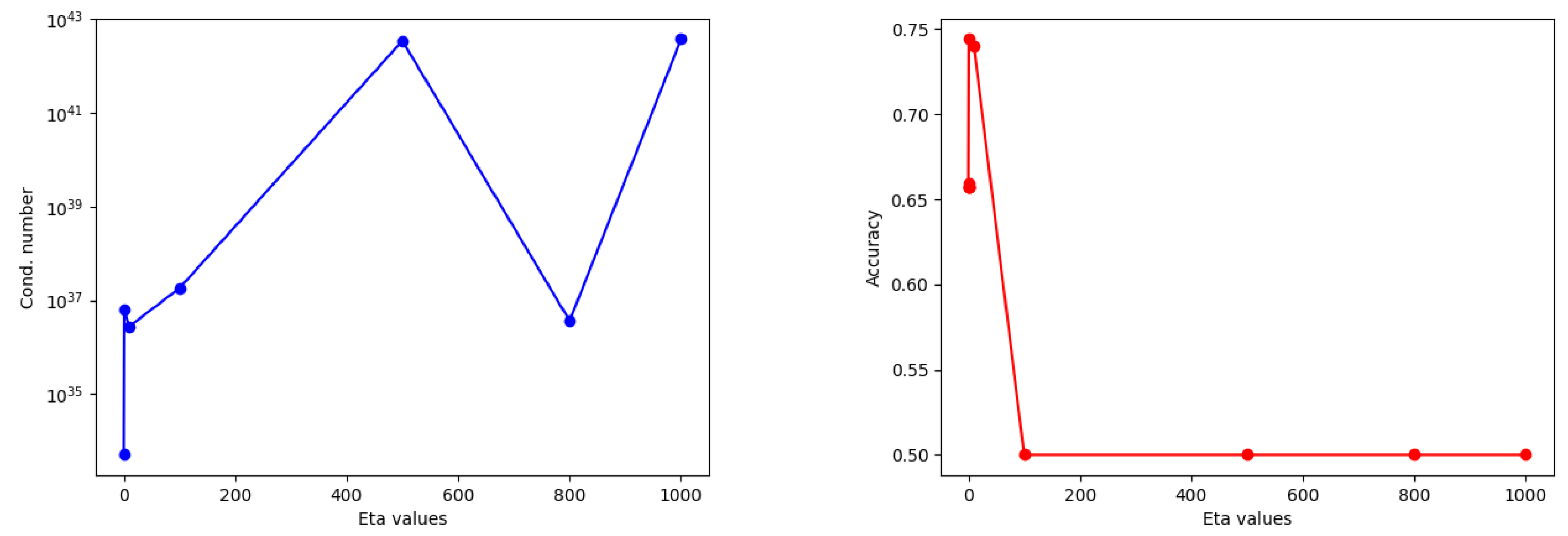
The PSSK has only one parameter to tune: $\sigma$. Typically, the users consider $\sigma \in \{0.001,0.01,0.1,1,10,100,1000\}$. We ran the CV phase for different shuffles of a dataset and plotted the results in terms of the condition number of the Gram matrix related to the training samples and the accuracy. For our analysis, we considered $\sigma \in \{0.00001,0.0001,0.001,$$0.01,0.1,1,10,100,500,800,1000\}$ and we ran tests on some datasets cited in the following. The results were similar in each case, so we decided to report those for the SHREC14 dataset.

From the Figure 4, it is evident that large values of $\sigma$ result in an unstable matrix and less accuracy. Then, in what follows, we will take into account only $\sigma \in \{0.00001,0.0001,$$0.001,0.01,0.1,1,10\}$.

The PWGK is the kernel with a higher number of parameters to tune; therefore, it was not so evident what were the best-set values to take into account. We chose reasonable starting sets as follows: $\tau \in \{0.001,0.01,0.1,1,10,100,1000\}$, $\rho \in \{0.001,0.01,0.1,1,10,100,1000\}$, $p\in \{1,5,10,50,100\}$, $C_w\in \{0.001,0.01,0.1,1\}$. Due to a large number of parameters, we first ran some experiments varying $(\rho ,\tau )$ with fixed $(p,C_w)$, and then we reversed the roles.

We report here in Figure 5 only a plot for fixed $C_w$ and p because this highlights how high values of $\tau$ (for example $\tau =1000$) were excluded. We found this behavior for different values of $C_w,p$ and various datasets—here, for the case $C_w=1$, $p=10$ and the MUTAG dataset. Therefore, we decided to vary the parameters, as follows: $\tau \in \{0.001,0.01,0.1,1,10,100\}$, $\rho \in \{0.001,0.01,0.1,1,10,100,1000\}$, $p\in \{1,5,10,50,100\}$, $C_w\in \{0.001,0.01,0.1,1\}$. Unfortunately, there was no other evidence that could guide the choices, except for $\tau$, where values $\tau =1000$ always had bad accuracy, as one can see below in the case of MUTAG with the shortest path distance.

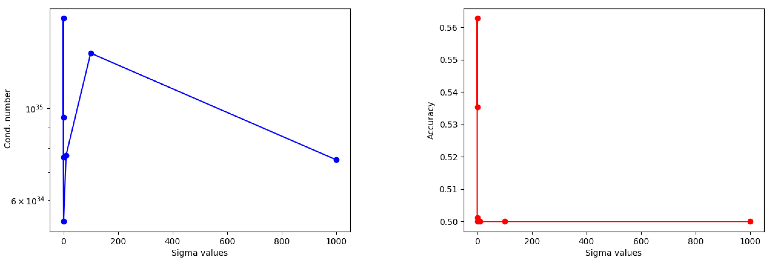
In the case of the SWK, there is only one parameter, $\eta$. In [11], the authors proposed to consider values starting from the first and last decile and with the median value of the gram matrix of the training samples flattened, in order to obtain a vector; then, they multiplied these three values for $0.01,0.1,1,10,100$.

For our analysis, we decided to study the behavior of such kernels, considering the same set of values independently from the specific dataset. We considered $\eta \in \{0.00001,0.0001,0.001,0.01,0.1,1,10,100,500,800,1000\}$.

We ran tests on some datasets, and the plot, related to the DHFR dataset, revealed evidently that large values for $\eta$ were to be excluded, as suggested by Figure 6. So, we decided to take $\eta$ only in $\{0.00001,0.0001,0.001,0.01,0.1,1,10\}$.

The PFK has two parameters: the variance $\sigma$ and t. In [12], the authors exhibited the procedure to follow, in order to obtain the corresponding set of values. It shows that the choice of t depends on $\sigma$. Our aim in this paper was to carry out an analysis that was dataset-independent, which turned out to be strictly connected only to the definition of the kernel itself. First, we took different values for $(\sigma ,t)$ and we plotted the corresponding accuracies—here, in the case of MUTAG with the shortest path distance, but the same behavior holds true also for other datasets.

The condition numbers were indeed high for every choice of parameters and, therefore, we avoided reporting here, because it would have been meaningless. From the Figure 7, it is evident that it is convenient to set $\sigma$ lower or equal to 10, while t should be set larger or equal to 0.1. Thus, in what follows, we took into account $\sigma \in \{0.001,0.01,0.1,1,10\}$ and $t\in \{0.1,1,10,100,1000\}$.

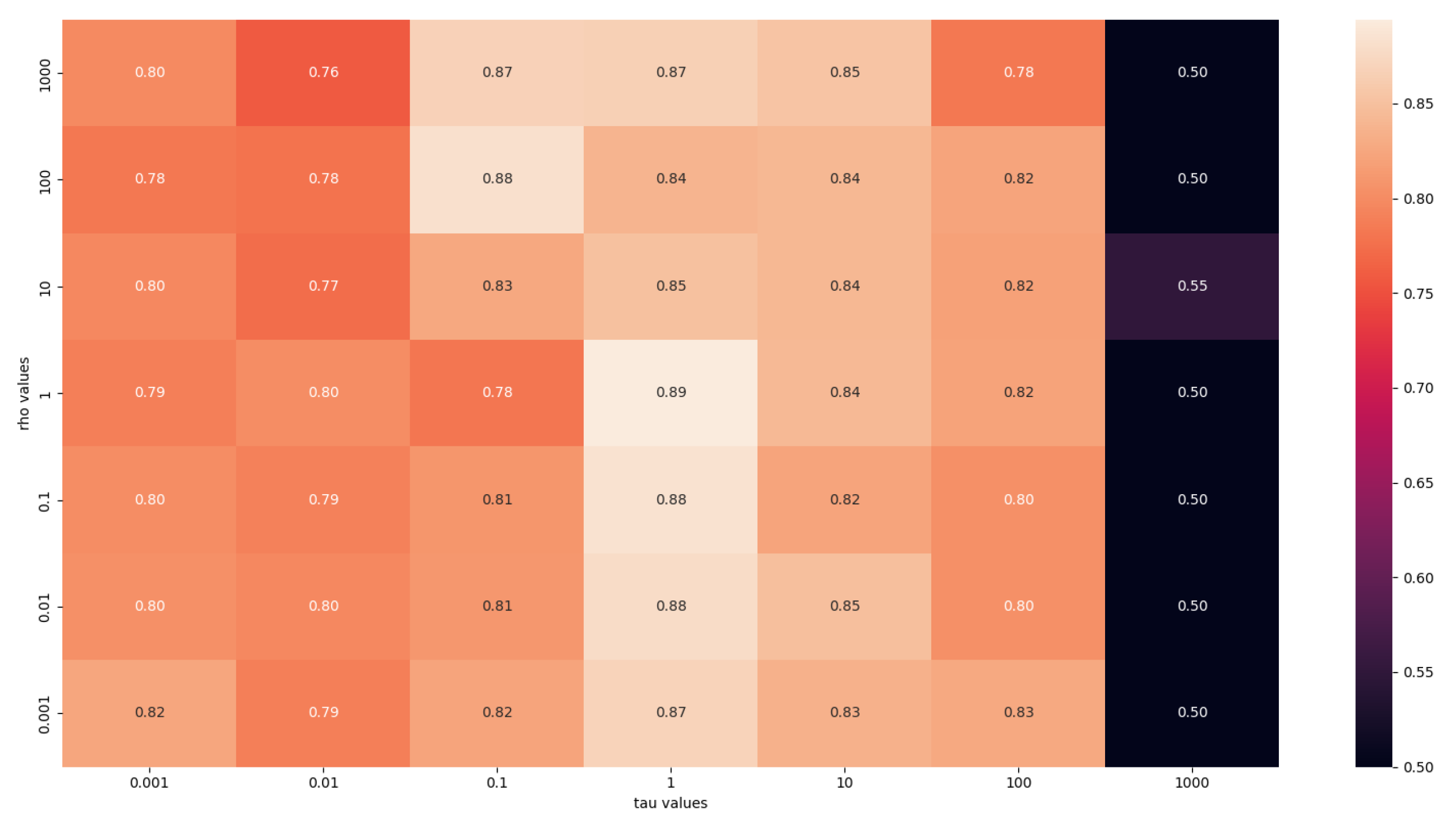
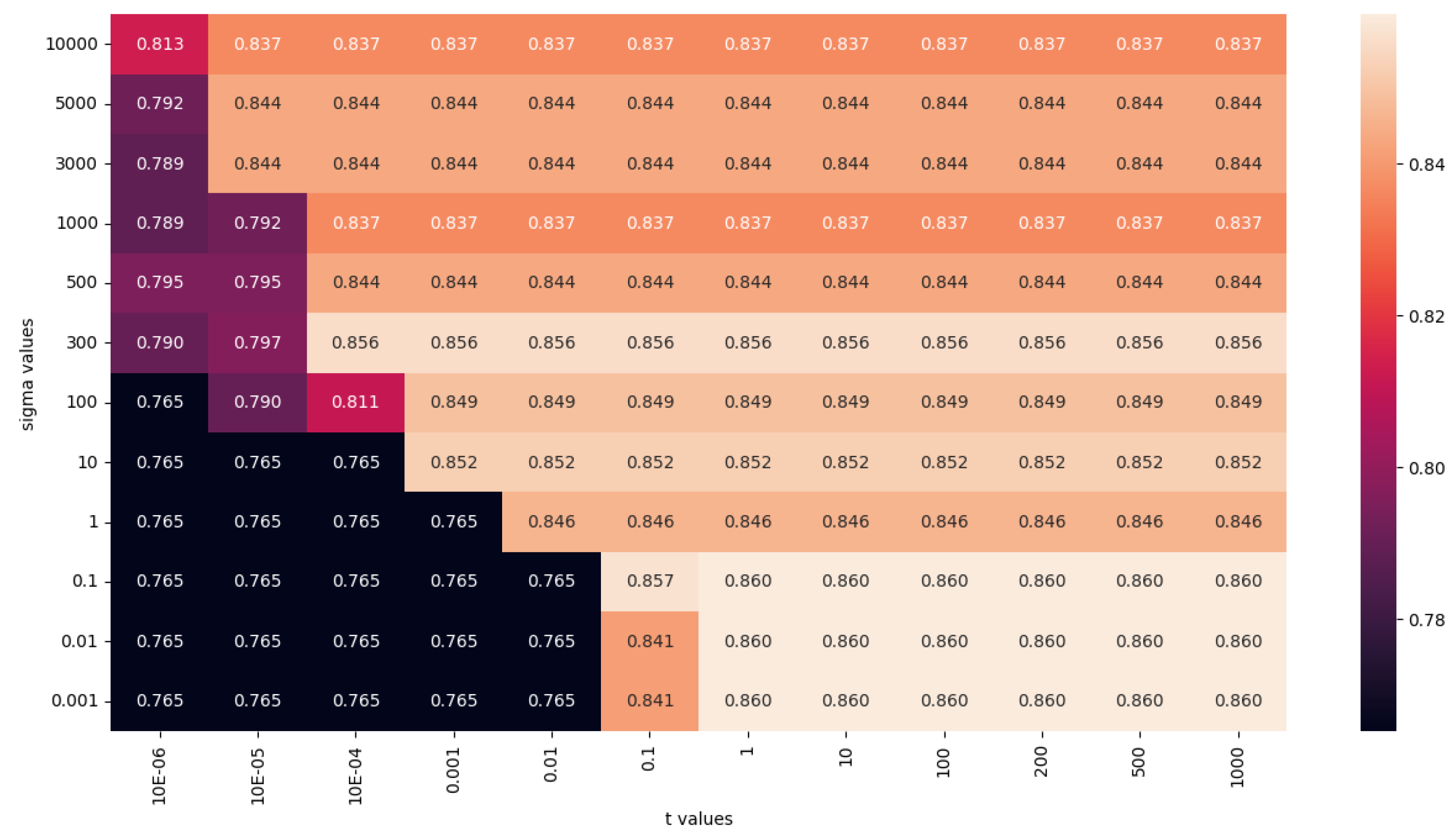
In the case of the PI, we considered a reasonable set of values for the parameter $\sigma \in \{0.001,0.01,0.1,1,10,100,1000\}$. The results were related to BZR with the shortest path distance redand shown in Figure 8.

As in the previous kernels, it seemed that the accuracy was better for small values of $\sigma$. For this reason, we set $\sigma \in \{0.000001,0.00001,0.0001,0.001,0.01,0.1,1,10\}$.

3.2. Numerical Tests

For what concerned the computation of simplicial complexes and persistence diagrams, we used some Python libraries available online: gudhi [26], ripser [27], giotto-tda [28] and persim [29]. On all the datasets, we performed a random splitting $(70\%/30\%)$ for training and testing, and we applied a tenfold cross-validation on the training set, in order to tune the parameters. Then, we averaged the results over 10 runs. For balanced datasets, we measured the performances of the classifier through accuracy for binary and multiclass problems:

$$\mathrm{accuracy}={\displaystyle \frac{\mathrm{number}\mathrm{of}\mathrm{test}\mathrm{samples}\mathrm{correctly}\mathrm{classify}}{\mathrm{all}\mathrm{test}\mathrm{samples}}}$$

In the case of the imbalanced datasets, we adopted balanced accuracy, as explained in [30]: if for every class i we defined the related recall as

$$recal{l}_i={\displaystyle \frac{\mathrm{test}\mathrm{samples}\mathrm{of}\mathrm{class}\mathrm{i}\mathrm{correctly}\mathrm{classify}}{\mathrm{all}\mathrm{test}\mathrm{samples}\mathrm{of}\mathrm{class}\mathrm{i}}}$$

then the balanced accuracy in the case of n different classes was

$$\text{balanced\_accuracy}={\displaystyle \frac{{\sum }_{i=1}^{n}recal{l}_i}{n}}$$

This definition was able to effectively quantify how accurate the classifier was, even in the case of the smallest classes. For the tests, we used the implementation of the SVM provided by the Scikit [31] library of Python. For PFK, we precomputed the Gram matrices using a Matlab (Matlab R2023b) routine because it is faster than the Python one. The values for C belonged to $\{0.001,0.01,0.1,1,10,100\}$. For each kernel, we considered the following values for the parameters:

• PSSK: $\sigma \in \{0.00001,0.0001,0.001,0.01,0.1,1,10\}$.
• PWGK: $\tau \in \{0.001,0.01,0.1,1,10,100\}$, $\rho \in \{0.001,0.01,0.1,1,10,100,1000\}$, $p\in \{1,5,10,50,100\}$, $C_w\in \{0.001,0.01,0.1,1\}$, and for the kernel we chose the Gaussian one.
• SWK: $\eta \in \{0.00001,0.0001,0.001,0.01,0.1,1,10\}$.
• PFK: $\sigma \in \{0.001,0.01,0.1,1,10\}$ and $t\in \{0.1,1,10,100,1000\}$.
• PI: $\sigma \in \{0.000001,0.00001,0.0001,0.001,0.01,0.1,1,10\}$ and number of pixel 0.1.

All the codes were run using Python 3.11 on a 2.5 GHz Dual-Core Intel Core i5, 32 Giga RAM. They can be found and downloaded from the GitHub page https://github.com/cinziabandiziol/persistence_kernels (accessed on 1 August 2024).

3.3. Point Cloud Data and Shapes

3.3.1. Protein

This is the Protein Classification Benchmark dataset PCB00019 [32]. It sums up information for 1357 proteins related to 55 classification problems. The data were highly imbalanced and therefore we applied the classifier to one of them, whereby the imbalance was slightly less evident. Persistence diagrams were computed for each protein by considering the 3-D structure or, better still, the $(x,y,z)$ position of any atoms in each of the 1357 molecules, as a point cloud in ${\mathbb{R}}^3$. Finally, using ripser we computed the persistence diagrams of only one dimension.

3.3.2. SHREC14—Synthetic Data

This dataset is related to the problem of non-rigid 3D shape retrieval. It collects exclusively human models in different body shapes and 20 poses, some examples are reported in Figure 9. It consists of 15 different human models, including man, woman, and child, each with its own body shape. Each of these models exists in 20 different poses, making up a dataset composed of 300 models.

For each shape, the meshes are given with about 60,000 vertices and, using the Heat Kernel Signature (HKS) introduced in [33], over different values of $t_i$ as [8], we computed the persistence diagrams of the induced filtrations in dimensions 1.

3.3.3. Orbit Recognition

We considered the dataset proposed in [13]. We took into account the linked twisted map, which modeled the fluid flows. The orbits could then be computed through the following discrete dynamical system:

$$\left\{\begin{array}{cc}{x}_{n+1}\hfill & =x_n+r{y}_n(1-y_n)\mathrm{mod}1\hfill \\ y_{n+1}\hfill & =y_n+r{x}_{n+1}(1-x_{n+1})\mathrm{mod}1\hfill \end{array}\right.$$

with the starting point $(x_0,y_0)\in [0,1]\times [0,1]$ and $r>0$ being a real number that influenced the behavior of the orbits, as shown in Figure 10.

As in [13], $r\in 2.5,3.5,4,4.1,4.3$, and it was strictly connected to the label of the corresponding orbit. For each of them, we provided the first 1000 points of 50 orbits, with starting points chosen randomly. The final dataset was composed of 250 elements. We computed the PDs, considering only the one-dimensional features. Since each PD had a huge number of topological features, we decided to consider only the first 10 most persistent ones, as in [15].

Firstly, the great difference in performances among the different datasets was probably due to the high imbalance of the PROTEIN one, with respect to the perfect balance of the other ones. It is well-known that if the classifier does not have enough samples for each class, as in the case of the imbalanced dataset, it has to face significant issues in classifying correctly the elements of the minor classes. From

Table 1. Accuracy related to point cloud and shape datasets (Balanced Accuracy only for the PROTEIN dataset). The best results are underlined in bold.

Kernel	PROTEIN	SHREC14	DYN SYS
PSSK	0.561	0.933	0.829
PWGK	0.538	0.923	0.819
SWK	0.531	0.935	0.841
PFK	0.556	0.935	0.784
PI	0.560	0.934	0.777

it is evident how, except for PROTEIN, where the PSSK showed slightly better performances, for SHREC14 and DYN SYS the best accuracy was achieved by the SWK.

3.4. Images

All the definitions introduced in Section 2 can be extended to another kind of simplicial complex, the cubical complex. This is useful when one deals with images or objects based on meshes, for example. More details can be found in [34].

Definition 14. 

An elementary cube $Q\subset {\mathbb{R}}^d$ can be defined as the product of $I_1$, $Q=I_1\times \cdots \times I_d$, where each $I_j$ can be either a set with one element $\left\{m\right\}$ or a unit-length interval $[m;m+1]$ for some $m\in \mathbb{Z}.$ A k-cube Q is a cube whose number of unit-length intervals in the product of Q is equal to k, which is then defined as the dimension of the cube Q. If $Q_1$ and $Q_2$ are cubes and $Q_1\subset Q_2$ then $Q_1$ is called a face of $\overline{Q}$. A cubical complex X in ${\mathbb{R}}^d$ is a collection of k-cubes $(0\le k\le d)$, such that:

• every face of a cube in X has to belong to X;
• given two cubes of X, their intersection must be either empty or a face of each of them.

The lower dimensional cubical complexes are reported in Figure 11.

MNIST and FMNIST

MNIST [35] is very common in the classification framework. It consists of 70,000 handwritten digits, in grayscale as one can see in Figure 12, which one can try to classify into 10 different classes. Each image can be viewed as a set of pixels with a value between 0 and 256 (black and white), as in the figure below:

Starting from this kind of dataset, we have to compute the corresponding persistent features. According to the approach proposed in [36] coming from [9], we first binarize each image: for instance, we replace each grayscale image with a white/black one, then we use as a filtration function the so-called Height filtration $\mathcal{H}\left(p\right)$ in [36]. For a cubical complex, for a chosen vector $v\in {\mathbb{R}}^d$ of unit norm, it is defined as

$$\mathcal{H}\left(p\right)=\left\{\begin{array}{cc}\langle p,v\rangle \hfill & \mathrm{if}p\mathrm{is}\mathrm{black},\hfill \\ H_{\infty }\hfill & \mathrm{otherwise}\hfill \end{array}\right.$$

where $H_{\infty }$ is a large default value chosen by the user. As in [9], we choose four different vectors for p, $(1,0),(-1,0),(0,1),(0,-1)$, and we compute zero and one-dimensional persistent features, using both the tda-giotto and the gudhi libraries. Finally, we concatenate them. For the current experiment, we decided to focus the test on a subset of the original MNIST, composed of only 10,000 samples. This was a balanced dataset. Due to some memory issues, we had to consider for this dataset a pixel size of $0.5$ and for the PWGK only $\tau \in \{0.001,0.01,0.1,1,10,100\}$, $\rho \in \{0.001,0.1,10,1000\}$, $p=10$, $C_w\in \{0.001,0.01,0.1,1\}$.

Another example of a grayscale image dataset is the FMNIST [37], which contains 28 × 28 grayscale images related to the fashion world. Figure 13 shows an example.

To deal with this, we followed another approach proposed in [23], where the authors applied padding, median filter, shallow thresholding and canny edges and then computed the usual filtration to the image obtained. Due to some memory issues, we had to consider for this dataset a pixel size of 1 and for the PWGK only $\tau \in \{0.001,0.01,0.1,1,10,100\}$, $\rho \in \{0.001,0.1,10,1000\}$, $p=10$, $C_w\in \{0.001,0.01,0.1,1\}$.

Both datasets were balanced, and it is probable that the results were better in the case of MNIST, due the fact that it is easier to classify handwritten digits instead of images of cloths. The SWK showed a slightly better performance as reported in

Table 2. Accuracy related to MNIST and FMNIST. The best results are underlined in bold.

Kernel	MNIST	FMNIST
PSSK	0.729	0.664
PWGK	0.754	0.684
SWK	0.802	0.709
PFK	0.734	0.671
PI	0.760	0.651

.

3.5. Graphs

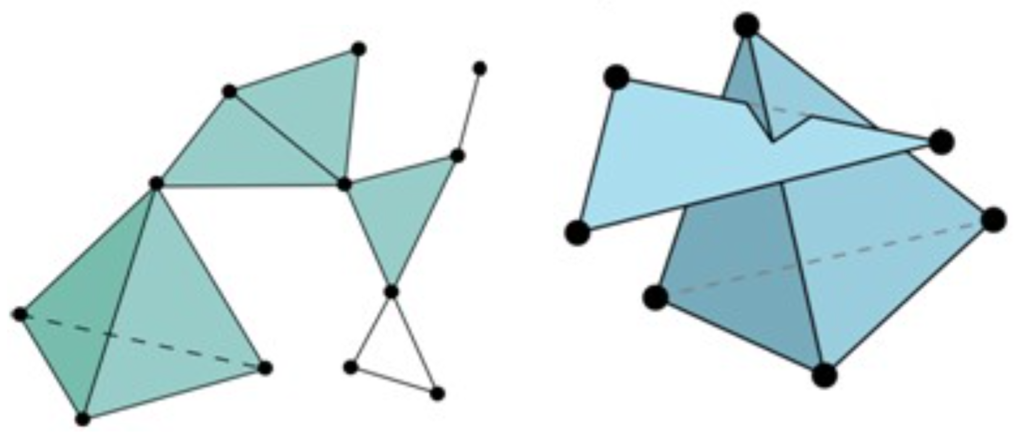
In many different contexts, from medicine to chemistry, data can have the structure of graphs. Graphs are couples of a set $(V,E)$, where V is the set of vertices and E is the set of edges. The graph classification is the task of attaching a label/class to each whole graph. In order to compute the persistent features, we needed to build a filtration. In the context of graphs, as in other cases, there are different definitions; see, for example, in [38].

We considered the Vietoris–Rips filtration, where, starting from the set of vertices, at each step we would add the corresponding edge whose weights were less or equal to a current value $ϵ$. This turned out to be the most common choice, and the software available online allowed us to build it after providing the corresponding adjacency matrix. In our experiments, we considered only undirected graphs, but, as in [38], building a filtration is possible also for directed graphs. Once defining the kind of filtration to use, one needs again to choose the corresponding weights. We decided to take into account first the shortest path distance and then the Jaccard index, as, for example, in [14].

Given two vertices $u,v\in V$ the shortest path distance was defined as the minimum number of different edges that one has to meet going from u to v or vice versa, since the graphs here were considered as undirected. In graphs theory, this is a widely use metric.

The Jaccard index is a good measure of edge similarity. Given an edge $e=(u,v)\in E$ then the corresponding Jaccard index is computed as

$$\rho (u,v)=\left|{\displaystyle \frac{NB\left(u\right)\cap NB\left(v\right)}{NB\left(u\right)\cup NB\left(v\right)}}\right|$$

where $NB\left(u\right)$ is the set of neighbors of u in the graph. This metric recovers the local information of nodes, in the sense that two nodes are considered similar if their neighbor sets are similar.

In both cases, we considered the sub-level set filtration and we collected both zero- and one-dimensional persistent features.

We took six of such sets among the graph benchmark datasets, all undirected, as follows:

• MUTAG: a collection of nitroaromatic compounds, the goal being to predict their mutagenicity on Salmonella typhimurium;
• PTC: a collection of chemical compounds represented as graphs that report the carcinogenicity of rats;
• BZR: a collection of chemical compounds that one has to classify as active or inactive;
• ENZYMES: a dataset of protein tertiary structures obtained from the BRENDA enzyme database; the aim is to classify each graph into six enzymes;
• DHFR: a collection of chemical compounds that one has to classify as active or inactive;
• PROTEINS: in each graph, nodes represent the secondary structure elements; the task is to predict whether or not a protein is an enzyme.

The properties of the above are summarized in

Table 3. Graph datasets.

Dataset	N° Graphs	N° Classes	IR
MUTAG	188	2	125:63
PTC	344	2	192:152
BZR	405	2	319:86
ENZYMES	600	6	100:100
DHFR	756	2	461:295
PROTEINS	1113	2	663:450

, where the IR index is the so-called Imbalanced Ratio (IR) that denotes the imbalance of the dataset, and it is defined as a sample size of the major class over a sample size of the minor class.

The computations of the adjacency matrix and the PDs were made using the functions implemented in tda-giotto.

The performances achieved with the two edge weights are reported in

Table 4. Balanced Accuracy related to graph datasets using the shortest path distance (for the ENZYMES dataset, Accuracy only). The best results are underlined in bold.

Kernel	MUTAG	PTC	BZR	DHFR	PROTEINS	ENZYMES
PSSK	0.868	0.545	0.606	0.557	0.668	0.281
PWGK	0.858	0.510	0.644	0.655	0.694	0.329
SWK	0.872	0.511	0.712	0.656	0.686	0.370
PFK	0.842	0.534	0.682	0.656	0.694	0.341
PI	0.863	0.542	0.585	0.519	0.691	0.285

and

Table 5. Balanced Accuracy related to graph datasets using the Jaccard Index (for the ENZYMES dataset, Accuracy only) The best results are underlined in bold.

Kernel	MUTAG	PTC	BZR	DHFR	PROTEINS	ENZYMES
PSSK	0.865	0.490	0.704	0.717	0.675	0.298
PWGK	0.859	0.516	0.720	0.727	0.699	0.355
SWK	0.858	0.523	0.703	0.726	0.689	0.406
PFK	0.874	0.554	0.704	0.743	0.678	0.400
PI	0.846	0.478	0.670	0.712	0.690	0.280

.

Thanks to these results, two conclusions can be reached. The first one is that, as expected, the goodness of the classifier is strictly related to the particular filtration used for the computation of persistent features. The second one is related to the fact that the SWK and the PFK seem to work slightly better than the other kernels: in the case of the shortest path distance in Table 4, the SWK is to be preferred while the PFK seems to work better in the case of the Jaccard index Table 5. In the case of PROTEINS, in both cases the PWGK provides the best Balanced Accuracy.

3.6. One-Dimensional Time Series

In many different applications, one can deal with one-dimensional time series. A one-dimensional time series is a set $\{x_t\in \mathbb{R}|t=1,\dots ,T\}$. In [39], the authors provided different approaches to building a filtration upon this kind of data. We decided to adopt the most common one. Thanks to the Taken’s embedding, these data could be translated into point clouds. With suitable choices for two parameters—$\tau >0$ for the delay parameter and $d>0$ for the dimension—it was possible to compute a subset of points in ${\mathbb{R}}^d$ composed by $v_i=\{x_i,x_{i+\tau },\dots ,x_{i+(d-1)\tau }\}$ for $i=1,\dots ,T-(d-1)\tau$. The theory mentioned above related to point clouds could then be applied to signals, as points in ${\mathbb{R}}^d$. For how to choose values for the parameters, see [39]. The datasets for the tests, in

Table 6. Time series datasets.

Dataset	N° Time Series	N° Classes	IR
ECG200	200	2	133:67
SONY	621	2	349:272
DISTAL	876	2	539:337
STRAWBERRY	983	2	632:351
POWER	1096	2	549:547
MOTE	1272	2	685:587

, were taken from the UCR Time Series Classification Archive (2018) [40], which consists of 128 datasets of time series from different worlds of application. In the archive, there is a split into test and train sets, but for the aim of our analysis we did not regard the split; we considered the train and test data as a whole dataset and then the codes provided properly the subdivision.

Using giotto-tda, we computed the persistent features of zero, one and two dimensions and joined them together. The final results of the datasets are reported in

Table 7. Balanced Accuracy related to time series datasets. The best results are underlined in bold.

Kernel	ECG200	SONY	DISTAL	STRAWBERRY	POWER	MOTE
PSSK	0.642	0.874	0.658	0.814	0.720	0.618
PWGK	0.726	0.888	0.696	0.892	0.769	0.633
SWK	0.731	0.892	0.723	0.898	0.784	0.671
PFK	0.707	0.895	0.676	0.892	0.750	0.652
PI	0.717	0.841	0.662	0.793	0.712	0.606

.

As in the previous examples, the SWK achieved the best results and provided slightly better performances, in terms of accuracy.

4. Discussion

In this paper, we compared the performances of five Persistent Kernels applied to data of different natures. The results show how different PKs are indeed comparable, in terms of accuracy, and that there was no one PK that emerged clearly above the others. However, in many cases, the SWK and PFK performed slightly better. In addition, from a purely computational point of view, the SWK is to be preferred, since by construction the preGram matrix is parameter-independent. Therefore, in practice, the user has to compute such a matrix on the whole dataset only once at the beginning and then choose a suitable subset of rows and columns to perform the training, cross-validation and test phases. This aspect is relevant and reduces the computational costs and time compared with other kernels. Another aspect to be considered, as in the case of graphs, is how to choose the function f that provides the filtration. The choice of such a function is still an open problem and an interesting field of research. The right choice, in fact, would guarantee being able to better extract the intrinsic information from data, thus improving the classifier’s performances. For the sake of completeness, we recall here that in the literature there is also an interesting direction of research, the aim of which is to build a new PK starting from the main five kernels that we introduced in Section 2.3. From one of the PKs mentioned in previous sections, the authors in [15,41] studied how to modify them, obtaining the so-called Variably Scaled Persistent Kernels, which are Variably Scaled Kernels applied to the classification context. The results reported by the authors are indeed promising. This could, therefore, be another interesting direction for further analysis.