The Local Convergence of a Three-Step Sixth-Order Iterative Approach with the Basin of Attraction

Abstract

In this study, we introduce an iterative approach exhibiting sixth-order convergence for the solution of nonlinear equations. The method attains sixth-order convergence by using three evaluations of the function and two evaluations of the first-order derivative per iteration. We examined the theoretical convergence of our method through the convergence theorem, which substantiates the convergence order. Furthermore, we analyzed the local convergence of our proposed technique by employing a hypothesis that involves the first-order derivative of the function $\Theta$ alongside the Lipschitz conditions. To evaluate the performance and efficacy of our iterative method, we provide a comparative analysis against existing methods based on various standard numerical problems. Finally, graphical comparisons employing basins of attraction are presented to illustrate the dynamic behavior of the iterative method in the complex plane.

1. Introduction

Many problems in science and engineering involve nonlinear equations, which are in the form

$$\Theta \left(\alpha \right)=0$$

(1)

where $\Theta$ is a differentiable function defined on a convex subset $\mathbb{D}$ of $\mathbb{S}$ with the values in $\mathbb{S}$, where $\mathbb{S}$ is $\mathbb{R}$ or $\mathbb{C}$. Many equations for real-world issues are too complicated and are hard to solve with an analytical approach. Therefore, researchers have focused on iterative methods.

Iterative-root-finding techniques are essential for approximating solutions to nonlinear equations in the field of nonlinear analysis. These techniques provide important resources for approximating solutions in a variety of disciplines, including computer science, physics, engineering, and economics. Alternatively, optimization algorithms have been used to find solutions for nonlinear equations or systems of nonlinear equations. Over the past ten years, many new optimization algorithms [1] have been developed. By enhancing these algorithms’ performance, researchers have achieved more accurate solutions. Numerical instability may arise during the computation of certain problems; at that time, the iterative methods can be designed to improve numerical stability and prevent divergence. One of the basic iteration formulas for finding the approximate root of the nonlinear Equation (1) is the well-known Newton–Raphson method, which is given by

$${\alpha }_{n+1}={\alpha }_n-\frac{\mathsf{\Theta }\left({\alpha }_n\right)}{{\mathsf{\Theta }}^{\prime }\left({\alpha }_n\right)}$$

(2)

This method is known for its quadratic convergence. To enhance the efficiency and order of convergence [2], many scholars have introduced iterative techniques with a higher order of convergence and higher efficiency. Several important methods with third-order convergence are given in [3,4,5]; some of the important methods with fourth-order convergence are given in [6,7]; an important method with fifth-order convergence is given in [8,9]. Inspired by these directions, we aim to introduce a sixth-order iterative technique.

In the context of convergence analysis, semilocal and local convergence analyses [10,11] play a crucial role in understanding the behavior of iterative algorithms. Semilocal and local convergence analyses allow for a thorough evaluation of how well an iterative algorithm performs in the vicinity of a solution. Semilocal convergence analysis provides information about the behavior of the iterative sequence and ensures its convergence in a specific domain depending on the initial assumptions. We are interested in local convergence analysis in this work because it gives us the domain of possible initial guesses around the exact solution. In addition, the domain gives us the freedom to choose the initial guess that guarantees convergence. Researchers can choose appropriate initial guesses to obtain convergence radii, optimize convergence parameters, and ensure the algorithm’s reliability in real-world applications across a variety of scientific and engineering domains with the help of these convergence analyses.

In this current research, we derive the new sixth-order iterative method for solving the nonlinear equations. This approach requires three function evaluations and two derivatives per iteration. The advantage of this technique is that it is a second-order derivative and parameter-free technique, which helps to reduce the computational cost.

The structure of this paper is outlined as follows: We present our proposed iterative method and examine the convergence analysis of this method in Section 2; we address the local convergence properties of our proposed iterative method in Section 3; we present numerical results in Section 4; we explore the basin of attraction in Section 5; finally, we summarize our findings in the concluding Section 6.

2. Proposed Iterative Method and Convergence Analysis

In this section, we propose a new sixth-order iterative method and we present the convergence analysis of (3).

$$\begin{array}{cc}\hfill {\beta }_n& ={\alpha }_n-\frac{\mathsf{\Theta }\left({\alpha }_n\right)}{{\mathsf{\Theta }}^{\prime }\left({\alpha }_n\right)},\hfill \\ \hfill {\gamma }_n& ={\alpha }_n-\frac{\mathsf{\Theta }\left({\alpha }_n\right)-\mathsf{\Theta }\left({\beta }_n\right)}{\mathsf{\Theta }\left({\alpha }_n\right)-2\mathsf{\Theta }\left({\beta }_n\right)}\frac{\mathsf{\Theta }\left({\alpha }_n\right)}{{\mathsf{\Theta }}^{\prime }\left({\alpha }_n\right)},\hfill \\ \hfill {\alpha }_{n+1}& ={\gamma }_n-\frac{\mathsf{\Theta }\left({\beta }_n\right)-\mathsf{\Theta }\left({\gamma }_n\right)}{\mathsf{\Theta }\left({\beta }_n\right)-2\mathsf{\Theta }\left({\gamma }_n\right)}\frac{\mathsf{\Theta }\left({\gamma }_n\right)}{{\mathsf{\Theta }}^{\prime }\left({\beta }_n\right)}.\hfill \end{array}$$

(3)

The new scheme (3) uses a total of five functional evaluations per iteration and attains the sixth-order convergence. The efficiency index of the method is ${\left(p\right)}^{\frac{1}{n}}$, where p is the order of convergence and n is the number of function evaluations. Then, the efficiency index of method (3) is $6^{\frac{1}{5}}=1.430969$. Many researchers have used various approximations and interpolations to develop optimal methods that reduce the number of functional evaluations per iteration. However, even if the number of functional evaluations is minimized, the number of algebraic operations may increase [12]. It may not reach the optimal standards as per the theory of the Kung–Traub conjecture; however, it still provides an effective alternative. When approximating the derivative of a function, the symmetrically divided difference operator plays a vital role. The advantage of the symmetrically divided differences is that, using this, we can develop derivative-free iterative methods, especially when the nonlinear operators are not differentiable or, in the other case, when the computation of the derivative is difficult or it is very expensive to derive the derivative.

Theorem 1.

Suppose that the function $\mathsf{\Theta }:\mathbb{D}\subseteq \mathbb{R}\to \mathbb{R}$ is sufficiently differentiable in an open neighborhood $\mathbb{D}$ of its zero ${\alpha }^{*}$. If an initial expression ${\alpha }_0$ is sufficiently close to the root ${\alpha }^{*}$, then the iterative method (3) attains the sixth-order convergence. It satisfies the following error equation:

$$e_{n+1}=\left({\mathsf{c}}_2^5-{\mathsf{c}}_2{\mathsf{c}}_3^2\right)e_n^6+O\left(e_n^7\right).$$

(4)

Proof. 

Let us assume that $e_n={\alpha }_n-{\alpha }^{*}$ and ${\mathsf{c}}_k=\frac{{\mathsf{\Theta }}^k\left({\alpha }^{*}\right)}{k!{\mathsf{\Theta }}^{\prime }\left({\alpha }^{*}\right)}$. Expanding $\mathsf{\Theta }$ near ${\alpha }^{*}$ by using the Taylor series, we obtain

$$\mathsf{\Theta }\left({\alpha }_n\right)={\mathsf{\Theta }}^{\prime }\left({\alpha }^{*}\right)\left[e_n+{\mathsf{c}}_2{e}_n^2+{\mathsf{c}}_3{e}_n^3+{\mathsf{c}}_4{e}_n^4+{\mathsf{c}}_5{e}_n^5+{\mathsf{c}}_6{e}_n^6+O\left(e_n^7\right)\right]$$

(5)

and

$${\mathsf{\Theta }}^{\prime }\left({\alpha }_n\right)={\mathsf{\Theta }}^{\prime }\left({\alpha }^{*}\right)\left[1+2{\mathsf{c}}_2{e}_n+3{\mathsf{c}}_3{e}_n^2+4{\mathsf{c}}_4{e}_n^3+5{\mathsf{c}}_4{e}_n^4+6{\mathsf{c}}_6{e}_n^5+O\left(e_n^6\right)\right].$$

(6)

From (5) and (6), we obtain

$$\begin{array}{ccc}\hfill \frac{\mathsf{\Theta }\left({\alpha }_n\right)}{{\mathsf{\Theta }}^{\prime }\left({\alpha }_n\right)}& =e_n-{\mathsf{c}}_2{e}_n^2+2({\mathsf{c}}_2^2-{\mathsf{c}}_3)e_n^3+(7{\mathsf{c}}_2{\mathsf{c}}_3+4{\mathsf{c}}_2^2-3{\mathsf{c}}_4)e_n^4+(8{\mathsf{c}}_2^4-20{\mathsf{c}}_2^2{\mathsf{c}}_3+10{\mathsf{c}}_2{\mathsf{c}}_4\hfill & \hfill +6{\mathsf{c}}_3^2-4{\mathsf{c}}_5)e_n^5+O\left(e_n^6\right).\end{array}$$

(7)

By substituting (7) into (3), we obtain

$$\begin{array}{ccc}\hfill {\beta }_n& ={\alpha }^{*}+{\mathsf{c}}_2{e}_n^2-2({\mathsf{c}}_2^2-{\mathsf{c}}_3)e_n^3-(7{\mathsf{c}}_2{\mathsf{c}}_3+4{\mathsf{c}}_2^2-3{\mathsf{c}}_4)e_n^4-(8{\mathsf{c}}_2^4-20{\mathsf{c}}_2^2{\mathsf{c}}_3+10{\mathsf{c}}_2{\mathsf{c}}_4+6{\mathsf{c}}_3^2-4{\mathsf{c}}_5)e_n^5\hfill & \hfill +O\left(e_n^6\right).\end{array}$$

(8)

Now, use the Taylor series expansion of $\mathsf{\Theta }\left({\beta }_n\right)$ around ${\alpha }^{*}$; we have

$$\begin{array}{ccc}\hfill \mathsf{\Theta }\left({\beta }_n\right)& ={\mathsf{\Theta }}^{\prime }\left({\alpha }^{*}\right)[{\mathsf{c}}_2{e}_n^2-2({\mathsf{c}}_2^2-{\mathsf{c}}_3)e_n^3-(7{\mathsf{c}}_2{\mathsf{c}}_3+4{\mathsf{c}}_2^2-3{\mathsf{c}}_4)e_n^4-(8{\mathsf{c}}_2^4-20{\mathsf{c}}_2^2{\mathsf{c}}_3+10{\mathsf{c}}_2{\mathsf{c}}_4\hfill & \hfill +6{\mathsf{c}}_3^2-4{\mathsf{c}}_5)e_n^5+O\left(e_n^6\right)].\end{array}$$

(9)

By adopting expressions (5), (6), and (9), we obtain

$$\begin{array}{c}\frac{\mathsf{\Theta }\left({\alpha }_n\right)-\mathsf{\Theta }\left({\beta }_n\right)}{\mathsf{\Theta }\left({\alpha }_n\right)-2\mathsf{\Theta }\left({\beta }_n\right)}\frac{\mathsf{\Theta }\left({\alpha }_n\right)}{{\mathsf{\Theta }}^{\prime }\left({\alpha }_n\right)}=e_n+\left({\mathsf{c}}_2{\mathsf{c}}_3-{\mathsf{c}}_2^3\right)e_n^4+2\left(2{\mathsf{c}}_2^4-4{\mathsf{c}}_3{\mathsf{c}}_2^2+{\mathsf{c}}_4{\mathsf{c}}_2+{\mathsf{c}}_3^2\right)e_n^5\\ +\left(-10{\mathsf{c}}_2^5+30{\mathsf{c}}_3{\mathsf{c}}_2^3-12{\mathsf{c}}_4{\mathsf{c}}_2^2+3\left({\mathsf{c}}_5-6{\mathsf{c}}_3^2\right){\mathsf{c}}_2+7{\mathsf{c}}_3{\mathsf{c}}_4\right)e_n^6+O\left(e_n^7\right)\end{array}$$

(10)

and

$$\begin{array}{c}{\gamma }_n={\alpha }^{*}+\left({\mathsf{c}}_2^3-{\mathsf{c}}_2{\mathsf{c}}_3\right)e_n^4-2\left(2{\mathsf{c}}_2^4-4{\mathsf{c}}_3{\mathsf{c}}_2^2+{\mathsf{c}}_4{\mathsf{c}}_2+{\mathsf{c}}_3^2\right)e_n^5\\ +\left(10{\mathsf{c}}_2^5-30{\mathsf{c}}_3{\mathsf{c}}_2^3+12{\mathsf{c}}_4{\mathsf{c}}_2^2-3({\mathsf{c}}_5-6{\mathsf{c}}_3^2){\mathsf{c}}_2-7{\mathsf{c}}_3{\mathsf{c}}_4\right)e_n^6+O\left(e_n^7\right).\end{array}$$

(11)

Now, we have

$$\begin{array}{c}\frac{\mathsf{\Theta }\left({\beta }_n\right)-\mathsf{\Theta }\left({\gamma }_n\right)}{\mathsf{\Theta }\left({\beta }_n\right)-2\mathsf{\Theta }\left({\gamma }_n\right)}\frac{\mathsf{\Theta }\left({\gamma }_n\right)}{{\mathsf{\Theta }}^{\prime }\left({\alpha }_n\right)}={\alpha }^{*}+\left(c_2^3-c_2{c}_3\right)e_n^4-2\left(2c_2^4-4c_3{c}_2^2+c_4{c}_2+c_3^2\right)e_n^5\\ +\left(9c_2^5-30c_3{c}_2^3+12c_4{c}_2^2+\left(19c_3^2-3c_5\right)c_2-7c_3{c}_4\right)e_n^6+O\left(e_n^7\right)\end{array}$$

(12)

Using expressions (11) and (12) in the third sub-step of method (3), we have

$$e_{n+1}=\left({\mathsf{c}}_2^5-{\mathsf{c}}_2{\mathsf{c}}_3^2\right)e_n^6+O\left(e_n^7\right).$$

(13)

Hence, the above error Equation (13) shows the sixth-order convergence. □

3. Local Convergence

In this section, we present the local convergence analysis of method (3). Let us assume that $U(v,r)$ and $\overline{U}(v,r)$ are open and closed balls, respectively, with center v and radius $r>0$. In addition, we chose ${\lambda }_0>0$, $\lambda >0$, and $M>0$ as the parameters with the constraint ${\lambda }_0\le \lambda$.

Theorem 2.

Let us suppose that $\mathsf{\Theta }:\mathbb{D}\subset \mathbb{S}\to \mathbb{S}$ is a differentiable function. Assume that there exists ${\alpha }^{*}\in \mathbb{D}$ and given parameters ${\lambda }_0>0,\lambda >0,M>0$ for each $\alpha ,\beta \in \mathbb{D}$ verifying the following:

$$\mathsf{\Theta }\left({\alpha }^{*}\right)=0,{\mathsf{\Theta }}^{\prime }{\left({\alpha }^{*}\right)}^{-1}\in L(\mathbb{S},\mathbb{S}),$$

$$|{\mathsf{\Theta }}^{\prime }{\left({\alpha }^{*}\right)}^{-1}({\mathsf{\Theta }}^{\prime }\left(\alpha \right)-{\mathsf{\Theta }}^{\prime }\left({\alpha }^{*}\right))|\le {\lambda }_0|\alpha -{\alpha }^{*}|,$$

(14)

$$|{\mathsf{\Theta }}^{\prime }{\left({\alpha }^{*}\right)}^{-1}({\mathsf{\Theta }}^{\prime }\left(\alpha \right)-{\mathsf{\Theta }}^{\prime }\left(\beta \right))|\le \lambda |\alpha -\beta |,$$

(15)

$$|{\mathsf{\Theta }}^{\prime }{\left({\alpha }^{*}\right)}^{-1}\left({\mathsf{\Theta }}^{\prime }\left(\alpha \right)\right)|\le M$$

(16)

and

$$\overline{U}({\alpha }^{*},r)\subseteq \mathbb{D}.$$

(17)

Therefore, the sequence generated by the method (3) for ${\alpha }_0\in U({\alpha }^{*},r)\setminus {\alpha }^{*}$ is well defined in $\overline{U}({\alpha }^{*},r)$ for each $n=0,1,2,3,\dots$. It converges to ${\alpha }^{*}$. r stands for the radius of convergence of (36). Moreover, the following estimates hold:

$$|{\beta }_n-{\alpha }^{*}|\le g_1\left(\right|{\alpha }_n-{\alpha }^{*}\left|\right)|{\alpha }_n-{\alpha }^{*}|<|{\alpha }_n-{\alpha }^{*}|<1,$$

(18)

$$|{\gamma }_n-{\alpha }^{*}|\le g_3\left(\right|{\alpha }_n-{\alpha }^{*}\left|\right)|{\alpha }_n-{\alpha }^{*}|<|{\alpha }_n-{\alpha }^{*}|<1$$

(19)

and

$$|{\alpha }_{n+1}-{\alpha }^{*}|\le g_6\left(\right|{\alpha }_n-{\alpha }^{*}\left|\right)|{\alpha }_n-{\alpha }^{*}|<|{\alpha }_n-{\alpha }^{*}|<1.$$

(20)

where r and $g_1,g_{3}and{g}_6$ are to be determined. Furthermore, suppose that there exists $R\in [r,\frac{2}{{\lambda }_0})$ such that $\overline{U}({\alpha }^{*},R)\subseteq \mathbb{D}$. Then, the limit point ${\alpha }^{*}$ is the only solution of $\mathsf{\Theta }\left(\alpha \right)=0$ in $\overline{U}({\alpha }^{*},R)$.

Proof. 

Let ${\alpha }_0$ is an initial point in the domain $\mathbb{D}$.

From condition (14), since ${\alpha }_0\in \mathbb{D}$, we have

$$\left|{\mathsf{\Theta }}^{\prime }{\left({\alpha }^{*}\right)}^{-1}\left({\mathsf{\Theta }}^{\prime }\left({\alpha }_0\right)-{\mathsf{\Theta }}^{\prime }\left({\alpha }^{*}\right)\right)\right|\le {\lambda }_0|{\alpha }_0-{\alpha }^{*}|.$$

(21)

Let us assume that $|{\alpha }_0-{\alpha }^{*}|<\frac{1}{{\lambda }_0}$, by using the Banach lemma. We obtain the following:

$$\left|{\mathsf{\Theta }}^{\prime }{\left({\alpha }^{*}\right)}^{-1}\left({\mathsf{\Theta }}^{\prime }\left({\alpha }_0\right)-{\mathsf{\Theta }}^{\prime }\left({\alpha }^{*}\right)\right)\right|<1,$$

$$|{\mathsf{\Theta }}^{\prime }{\left({\alpha }^{*}\right)}^{-1}{\mathsf{\Theta }}^{\prime }\left({\alpha }_0\right)-{\mathsf{\Theta }}^{\prime }{\left({\alpha }^{*}\right)}^{-1}{\mathsf{\Theta }}^{\prime }\left({\alpha }^{*}\right)|<1,$$

$$\left|{\mathsf{\Theta }}^{\prime }{\left({\alpha }_0\right)}^{-1}{\mathsf{\Theta }}^{\prime }{\left(\alpha \right)}^{*}\right|=\frac{1}{1-{\lambda }_0|{\alpha }_0-{\alpha }^{*}|}$$

(22)

and

$${\beta }_n={\alpha }_n-{\mathsf{\Theta }}^{\prime }{\left({\alpha }_n\right)}^{-1}\mathsf{\Theta }\left({\alpha }_n\right).$$

(23)

Using $n=0$ in (23), we obtain

$${\beta }_0={\alpha }_0-\frac{\mathsf{\Theta }\left({\alpha }_0\right)}{{\mathsf{\Theta }}^{\prime }\left({\alpha }_0\right)},$$

(24)

which further yield

$$\begin{array}{cc}\hfill {\beta }_0-{\alpha }^{*}& ={\alpha }_0-{\alpha }^{*}-{\mathsf{\Theta }}^{\prime }{\left({\alpha }_0\right)}^{-1}\mathsf{\Theta }\left({\alpha }_0\right)\hfill \\ \hfill & =({\alpha }_0-{\alpha }^{*})\left[{\mathsf{\Theta }}^{\prime }{\left({\alpha }_0\right)}^{-1}{\mathsf{\Theta }}^{\prime }\left({\alpha }_0\right)\right]-{\mathsf{\Theta }}^{\prime }{\left({\alpha }_0\right)}^{-1}\mathsf{\Theta }\left({\alpha }_0\right),\hfill \\ \hfill & =-{\mathsf{\Theta }}^{\prime }{\left({\alpha }_0\right)}^{-1}{\int }_0^1{\mathsf{\Theta }}^{\prime }({\alpha }^{*}+\mathsf{\Theta }({\alpha }_0-{\alpha }^{*}))d\mathsf{\Theta }({\alpha }_0-{\alpha }^{*})-{\mathsf{\Theta }}^{\prime }\left({\alpha }_0\right)({\alpha }_0-{\alpha }^{*}),\hfill \\ \hfill & -{\mathsf{\Theta }}^{\prime }{\left({\alpha }_0\right)}^{-1}{\int }_0^1\left[{\mathsf{\Theta }}^{\prime }({\alpha }^{*}+\mathsf{\Theta }({\alpha }_0-{\alpha }^{*}))-{\mathsf{\Theta }}^{\prime }\left({\alpha }_0\right)\right]d\mathsf{\Theta }({\alpha }_0-{\alpha }^{*}).\hfill \end{array}$$

(25)

Taking the norm on both sides, we have

$$\begin{array}{cc}\hfill |{\beta }_0-{\alpha }^{*}|& =|{\mathsf{\Theta }}^{\prime }{\left({\alpha }_0\right)}^{-1}{\int }_0^1\left[{\mathsf{\Theta }}^{\prime }({\alpha }^{*}+\mathsf{\Theta }({\alpha }_0-{\alpha }^{*}))-{\mathsf{\Theta }}^{\prime }\left({\alpha }_0\right)\right]d\mathsf{\Theta }({\alpha }_0-{\alpha }^{*})|\hfill \\ \hfill & =|{\mathsf{\Theta }}^{\prime }{\left({\alpha }_0\right)}^{-1}{\mathsf{\Theta }}^{\prime }\left({\alpha }^{*}\right)||{\alpha }_0-{\alpha }^{*}|\left|{\int }_0^1{\mathsf{\Theta }}^{\prime }{\left({\alpha }^{*}\right)}^{-1}\left[{\mathsf{\Theta }}^{\prime }({\alpha }^{*}+\mathsf{\Theta }({\alpha }_0-{\alpha }^{*}))-{\mathsf{\Theta }}^{\prime }\left({\alpha }_0\right)d\mathsf{\Theta }\right]\right|,\hfill \\ \hfill & \le \frac{\lambda {|({\alpha }_0-{\alpha }^{*})|}^2}{2\left(1-{\lambda }_0|({\alpha }_0-{\alpha }^{*})|\right)},\hfill \\ \hfill & \le g_1|{\alpha }_0-{\alpha }^{*}|({\alpha }_0-{\alpha }^{*}),\hfill \\ \hfill & \le |{\alpha }_0-{\alpha }^{*}|\le r.\hfill \end{array}$$

(26)

For $n=0$ and ${\beta }_0\in U({\alpha }^{*},r)$, we obtain

$$g_1\left(\left|{\alpha }_0-{\alpha }^{*}\right|\right)=\frac{\lambda \left|{\alpha }_0-{\alpha }^{*}\right|}{2(1-{\lambda }_0\left|{\alpha }_0-{\alpha }^{*}\right|)},$$

(27)

So, we define auxiliary function ${\sigma }_1$ and obtain the first condition for parameter r:

$$\begin{array}{cc}\hfill & {\sigma }_1\left(t\right)=g_1\left(t\right)-1,\hfill \\ \hfill & \lambda t-2+2{\lambda }_{0}t=0,\hfill \\ \hfill & t(\lambda +2{\lambda }_0)=2,\hfill \\ \hfill & t=\frac{2}{\lambda +2{\lambda }_0},\hfill \\ \hfill & r_1=\frac{2}{\lambda +2{\lambda }_0},\hfill \\ \hfill & r_1=\frac{2}{2{\lambda }_0+\lambda }<\frac{1}{{\lambda }_0},\hfill \\ \hfill & {\sigma }_1\left(0\right)=g_1\left(0\right)-1<0,\hfill \end{array}$$

where ${\sigma }_1\left(\frac{1}{{\lambda }_0}\right)\to \infty \mathrm{as}t\to {\left(\frac{1}{{\lambda }_0}\right)}^{-}.$ It follows from the intermediate value theorem that the function ${\sigma }_1$ has the smallest root $r_1$ in the interval $(0,\frac{1}{{\lambda }_0})$. This implies

$$0<r_1<\frac{1}{{\lambda }_0}$$

and

$$0<g_1\left(t\right)<1\forall t\in (0,r_1).$$

From the second step of (3), putting $n=0$, we obtain

$${\gamma }_0={\alpha }_0-{\left(\mathsf{\Theta }\left({\alpha }_0\right)-2\mathsf{\Theta }\left({\beta }_0\right)\right)}^{-1}\left(\mathsf{\Theta }\left({\alpha }_0\right)-\mathsf{\Theta }\left({\beta }_0\right)\right)\mathsf{\Theta }{\left({\alpha }_0\right)}^{-1}\mathsf{\Theta }\left({\alpha }_0\right).$$

(28)

Taking the norm on both sides of (28), we obtain

$$\begin{array}{cc}\hfill \left|{\gamma }_0-{\alpha }^{*}\right|& =\left|{\alpha }_0-{\alpha }^{*}-{\left(\mathsf{\Theta }\left({\alpha }_0\right)-2\mathsf{\Theta }\left({\beta }_0\right)\right)}^{-1}\left(\mathsf{\Theta }\left({\alpha }_0\right)-\mathsf{\Theta }\left({\beta }_0\right)\right)\mathsf{\Theta }{\left({\alpha }_0\right)}^{-1}\mathsf{\Theta }\left({\alpha }_0\right)\right|.\hfill \end{array}$$

Let us assume that $P={\mathsf{\Theta }}^{\prime }\left({\alpha }^{*}\right){)}^{-1}{({\alpha }_0-{\alpha }^{*})}^{-1}$ and $T=\mathsf{\Theta }({\alpha }_0)-2\mathsf{\Theta }({\beta }_0)$. Then, we have

$$\begin{array}{cc}\hfill \left|I-PT\right|& =\left|{\mathsf{\Theta }}^{\prime }{({\alpha }^{*})}^{-1}{({\alpha }_0-{\alpha }^{*})}^{-1}\left[\mathsf{\Theta }({\alpha }_0)-2\mathsf{\Theta }({\beta }_0)-{\mathsf{\Theta }}^{\prime }({\alpha }^{*})({\alpha }_0-{\alpha }^{*})\right]\right|\hfill \\ \hfill & =\left|{\mathsf{\Theta }}^{\prime }{({\alpha }^{*})}^{-1}{({\alpha }_0-{\alpha }^{*})}^{-1}\left[\mathsf{\Theta }({\alpha }_0)-\mathsf{\Theta }({\alpha }^{*})-{\mathsf{\Theta }}^{\prime }({\alpha }^{*})({\alpha }_0-{\alpha }^{*})-2\mathsf{\Theta }({\beta }_0)\right]\right|\hfill \\ \hfill & =\frac{1}{\left|({\alpha }_0-{\alpha }^{*})\right|}\left|{\mathsf{\Theta }}^{\prime }{({\alpha }^{*})}^{-1}\left[{\int }_0^1\left[{\mathsf{\Theta }}^{\prime }({\alpha }^{*}+\mathsf{\Theta }({\alpha }_0-{\alpha }^{*}))-{\mathsf{\Theta }}^{\prime }({\alpha }_0)\right]d\mathsf{\Theta }({\alpha }_0-{\alpha }^{*})-2\mathsf{\Theta }({\beta }_0)\right]\right|\hfill \\ \hfill & \le \frac{1}{\left|({\alpha }_0-{\alpha }^{*})\right|}\left|{\int }_0^1{\mathsf{\Theta }}^{\prime }{({\alpha }^{*})}^{-1}\left[{\mathsf{\Theta }}^{\prime }({\alpha }^{*}+\mathsf{\Theta }({\alpha }_0-{\alpha }^{*}))-{\mathsf{\Theta }}^{\prime }({\alpha }_0)\right]d\mathsf{\Theta }({\alpha }_0-{\alpha }^{*}))]\right|\hfill \\ & +\frac{2}{\left|({\alpha }_0-{\alpha }^{*})\right|}\left|{\mathsf{\Theta }}^{\prime }({\alpha }^{*}){)}^{-1}\mathsf{\Theta }({\beta }_0)\right|\hfill \\ \hfill & \le \frac{{\lambda }_0\left|{\alpha }_0-{\alpha }^{*}\right|}{2}+2M{g}_1(\left|{\alpha }_0-{\alpha }^{*}\right|)\left|{\alpha }_0-{\alpha }^{*}\right|)\frac{1}{\left|{\alpha }_0-{\alpha }^{*}\right|}\hfill \\ \hfill & \le \frac{{\lambda }_0\left|{\alpha }_0-{\alpha }^{*}\right|}{2}+2M\frac{\lambda \left|{\alpha }_0-{\alpha }^{*}\right|}{2(1-{\lambda }_0\left|{\alpha }_0-{\alpha }^{*}\right|)}\hfill \\ \hfill & =g_2(\left|{\alpha }_0-{\alpha }^{*}\right|)\hfill \\ \hfill & \le g_2(r)\hfill \\ \hfill & <1\hfill \end{array}$$

(29)

and

$$\begin{array}{cc}\hfill \left|{(\mathsf{\Theta }\left({\alpha }_0\right)-2\mathsf{\Theta }\left({\beta }_0\right))}^{-1}{\mathsf{\Theta }}^{\prime }\left({\alpha }^{*}\right)\right|& \le \frac{1}{\left|{\alpha }_0-{\alpha }^{*}\right|(1-g_2\left(\left|{\alpha }_0-{\alpha }^{*}\right|\right))},\hfill \end{array}$$

(30)

where

$$\begin{array}{cc}\hfill & g_2\left(t\right)=\frac{{\lambda }_{0}t}{2}+\frac{M\lambda }{1-{\lambda }_{0}t},\hfill \\ \hfill & {\sigma }_2\left(t\right)=g_2\left(t\right)-1\hfill \\ \hfill & 3{\lambda }_{0}t-{\lambda }_0^2{t}^2+2(M\lambda -1)=0,\hfill \\ \hfill & t=\frac{3{\lambda }_0\pm \sqrt{9{\lambda }_0^2+8M\lambda {\lambda }_0^2-8{\lambda }_0^2}}{2{\lambda }_0^2},\hfill \\ \hfill & t=\frac{3\pm \sqrt{1+8M\lambda }}{2{\lambda }_0},\hfill \\ \hfill & g_2\left(0\right)=M\lambda .\hfill \end{array}$$

Suppose that $M\lambda <1$, then

$$\begin{array}{cc}\hfill {\sigma }_2\left(0\right)& =g_2\left(0\right)-1<0,\hfill \\ \hfill {\sigma }_2\left(\frac{1}{{\lambda }_0}\right)& \to \infty ast\to {\left(\frac{1}{{\lambda }_0}\right)}^{-}.\hfill \end{array}$$

It follows from the intermediate value theorem that the function ${\sigma }_2$ has the smallest root $r_2$ in the interval $(0,\frac{1}{{\lambda }_0})$. This implies

$$0<r_2<\frac{1}{{\lambda }_0},$$

and

$$\begin{array}{cc}\hfill \left|{\gamma }_0-{\alpha }^{*}\right|& \le \left|{\alpha }_0-{\alpha }^{*}\right|+\left|{\mathsf{\Theta }}^{\prime }{\left({\alpha }^{*}\right)}^{-1}(\mathsf{\Theta }\left({\alpha }_0\right)-\mathsf{\Theta }\left({\beta }_0\right))\right|\left|{(\mathsf{\Theta }\left({\alpha }_0\right)-2\mathsf{\Theta }\left({\beta }_0\right))}^{-1}{\mathsf{\Theta }}^{\prime }\left({\alpha }^{*}\right)\right|\hfill \\ \hfill & \times \left|(\mathsf{\Theta }{\left({\alpha }_0\right)}^{-1}{\mathsf{\Theta }}^{\prime }\left({\alpha }^{*}\right)\right|\left|{\mathsf{\Theta }}^{\prime }{\left({\alpha }^{*}\right)}^{-1}{\mathsf{\Theta }}^{\prime }\left({\alpha }_0\right)\right|\hfill \\ \hfill & =\left|{\alpha }_0-{\alpha }^{*}\right|\left[1+\frac{M^2(1-g_1\left(\left|{\alpha }_0-{\alpha }^{*}\right|\right))}{\left|{\alpha }_0-{\alpha }^{*}\right|(1-g_2\left(\left|{\alpha }_0-{\alpha }^{*}\right|\right)(1-{\lambda }_0\left|{\alpha }_0-{\alpha }^{*}\right|}\right]\hfill \\ \hfill & =g_3\left(\left|{\alpha }_0-{\alpha }^{*}\right|\right)\left|{\alpha }_0-{\alpha }^{*}\right|\hfill \\ \hfill & \le \left|{\alpha }_0-{\alpha }^{*}\right|<r.\hfill \end{array}$$

(31)

Since, $\left|{\gamma }_0-{\alpha }^{*}\right|<r$, this implies ${\gamma }_0\in U({\alpha }^{*},r)$. Then, we obtain

$$\begin{array}{cc}\hfill & g_3\left(\left|{\alpha }_0-{\alpha }^{*}\right|\right)=\left|{\alpha }_0-{\alpha }^{*}\right|+\frac{M^2(1-g_1\left(\left|{\alpha }_0-{\alpha }^{*}\right|\right))}{(1-g_2\left(\left|{\alpha }_0-{\alpha }^{*}\right|\right))(1-{\lambda }_0\left|{\alpha }_0-{\alpha }^{*}\right|)}\hfill \\ \hfill & g_3\left(t\right)=t+\frac{M^2(1-g_1\left(t\right))}{(1-g_2\left(t\right)(1-{\lambda }_{0}t))},\hfill \\ \hfill & {\sigma }_3\left(t\right)=g_3\left(t\right)-1,\hfill \\ \hfill & {\sigma }_3\left(0\right)=g_3\left(0\right)-1<0,\hfill \end{array}$$

since ${\sigma }_3{\left(r_2\right)}^{-}\to \infty$ as $t\to r_2^{-}.$ It follows from the intermediate value theorem that the function ${\sigma }_3$ has the smallest root $r_3$ in the interval $(0,r_2)$. This implies

$$0<r_3<r_2$$

and

$$0<g_3\left(t\right)<1\forall t\in (0,r_2).$$

By using $n=0$, in the third step of (3), we obtain

$$\begin{array}{cc}\hfill {\alpha }_1& ={\gamma }_0-{\left(\mathsf{\Theta }\left({\beta }_0\right)-2\mathsf{\Theta }\left({\gamma }_0\right)\right)}^{-1}\left(\mathsf{\Theta }\left({\beta }_0\right)-\mathsf{\Theta }\left({\gamma }_0\right)\right){\left({\mathsf{\Theta }}^{\prime }\left({\beta }_0\right)\right)}^{-1}\mathsf{\Theta }\left({\gamma }_0\right),\hfill \\ \hfill {\alpha }_1-{\alpha }^{*}& ={\gamma }_0-{\alpha }^{*}-{\left(\mathsf{\Theta }\left({\beta }_0\right)-2\mathsf{\Theta }\left({\gamma }_0\right)\right)}^{-1}\left(\mathsf{\Theta }\left({\beta }_0\right)-\mathsf{\Theta }\left({\gamma }_0\right)\right){\left({\mathsf{\Theta }}^{\prime }\left({\beta }_0\right)\right)}^{-1}\mathsf{\Theta }\left({\gamma }_0\right).\hfill \end{array}$$

(32)

Let us assume the following:

$$\begin{array}{cc}\hfill P& ={\mathsf{\Theta }}^{\prime }{\left({\alpha }^{*}\right)}^{-1}{({\beta }_0-{\alpha }^{*})}^{-1},\hfill \\ \hfill T& =\mathsf{\Theta }\left({\beta }_0\right)-2\mathsf{\Theta }\left({\gamma }_0\right).\hfill \end{array}$$

Then, we obtain

$$\begin{array}{cc}\hfill \left|I-PT\right|& =\left|{\mathsf{\Theta }}^{\prime }{\left({\alpha }^{*}\right)}^{-1}{({\beta }_0-{\alpha }^{*})}^{-1}\left[\mathsf{\Theta }\left({\beta }_0\right)-2\mathsf{\Theta }\left({\gamma }_0\right)-{\mathsf{\Theta }}^{\prime }\left({\alpha }^{*}\right)({\beta }_0-{\alpha }^{*})\right]\right|\hfill \\ \hfill & =\frac{1}{|{\beta }_0-{\alpha }^{*}|}\left|{\mathsf{\Theta }}^{\prime }{\left({\alpha }^{*}\right)}^{-1}\left[{\int }_0^1\left[{\mathsf{\Theta }}^{\prime }\left({\alpha }^{*}+\mathsf{\Theta }({\beta }_0-{\alpha }^{*})\right)-{\mathsf{\Theta }}^{\prime }\left({\alpha }^{*}\right)\right]d\mathsf{\Theta }({\beta }_0-{\alpha }^{*})-2\mathsf{\Theta }\left({\gamma }_0\right)\right]\right|\hfill \\ \hfill & \le \frac{1}{|{\beta }_0-{\alpha }^{*}|}\left|{\int }_0^1{\mathsf{\Theta }}^{\prime }{\left({\alpha }^{*}\right)}^{-1}\left[{\mathsf{\Theta }}^{\prime }\left({\alpha }^{*}+\mathsf{\Theta }({\beta }_0-{\alpha }^{*})\right)-{\mathsf{\Theta }}^{\prime }\left({\alpha }^{*}\right)\right]d\mathsf{\Theta }({\beta }_0-{\alpha }^{*})]\right|\hfill \\ \hfill & +\frac{2}{|{\beta }_0-{\alpha }^{*}|}\left|{\mathsf{\Theta }}^{\prime }\left({\alpha }^{*}\right){)}^{-1}\mathsf{\Theta }\left({\gamma }_0\right)\right|\hfill \\ \hfill & \le \frac{{\lambda }_0|{\beta }_0-{\alpha }^{*}|}{2}+2M\frac{\left|{\gamma }_0-{\alpha }^{*}\right|}{\left|{\beta }_0-{\alpha }^{*}\right|}\hfill \\ \hfill & =\frac{{\lambda }_0{g}_1\left(\left|{\alpha }_0-{\alpha }^{*}\right|\right)\left|{\alpha }_0-{\alpha }^{*}\right|}{2}+2M\frac{g_3\left(\left|{\alpha }_0-{\alpha }^{*}\right|\right)}{g_1\left(\left|{\alpha }_0-{\alpha }^{*}\right|\right)}\hfill \\ \hfill & =g_4\left(\left|{\alpha }_0-{\alpha }^{*}\right|\right)<g_4\left(r\right)<1,\hfill \end{array}$$

(33)

where

$$\begin{array}{cc}\hfill & g_4\left(\left|{\alpha }_0-{\alpha }^{*}\right|\right)=\frac{{\lambda }_0{g}_1\left(\left|{\alpha }_0-{\alpha }^{*}\right|\right)\left|{\alpha }_0-{\alpha }^{*}\right|}{2}+2M\frac{g_3\left(\left|{\alpha }_0-{\alpha }^{*}\right|\right)}{g_1\left(\left|{\alpha }_0-{\alpha }^{*}\right|\right)},\hfill \\ \hfill & g_4\left(t\right)=\frac{{\lambda }_0{g}_1\left(t\right)t}{2}+2M\frac{g_3\left(t\right)}{g_1\left(t\right)},\hfill \\ \hfill & {\sigma }_4\left(t\right)=g_4\left(t\right)-1,\hfill \\ \hfill & {\sigma }_4\left(0\right)=g_4\left(0\right)-1<0,\hfill \end{array}$$

since ${\sigma }_4{\left({\lambda }_0\right)}^{-}\to \infty$ as $t\to \frac{1}{{\lambda }_0}$. It follows from the intermediate value theorem that the function ${\sigma }_4$ has the smallest root $r_4$ in the interval $(0,\frac{1}{{\lambda }_0})$. This implies

$$0<r_4<\frac{1}{{\lambda }_0}$$

which further provides

$$\begin{array}{cc}\hfill \left|I-PT\right|& =\left|{\mathsf{\Theta }}^{\prime }{\left({\alpha }^{*}\right)}^{-1}{\mathsf{\Theta }}^{\prime }\left({\alpha }^{*}\right)-{\mathsf{\Theta }}^{\prime }{\left({\alpha }^{*}\right)}^{-1}{\mathsf{\Theta }}^{\prime }\left({\beta }_0\right)\right|\hfill \\ \hfill & =\left|{\mathsf{\Theta }}^{\prime }{\left({\alpha }^{*}\right)}^{-1}\left[{\mathsf{\Theta }}^{\prime }\left({\beta }_0\right)-{\mathsf{\Theta }}^{\prime }\left({\alpha }^{*}\right)\right]\right|\hfill \\ \hfill & \le \lambda \left|{\beta }_0-{\alpha }^{*}\right|\hfill \\ \hfill & \le \lambda g_1\left(\left|{\alpha }_0-{\alpha }^{*}\right|\right)\left|{\alpha }_0-{\alpha }^{*}\right|\hfill \\ \hfill & <1,\hfill \end{array}$$

(34)

where

$$\begin{array}{cc}\hfill & g_5\left(\left|{\alpha }_0-{\alpha }^{*}\right|\right)=\lambda \left|{\alpha }_0-{\alpha }^{*}\right|,\hfill \\ \hfill & g_5\left(t\right)=\lambda t,\hfill \\ \hfill & {\sigma }_5\left(t\right)=g_5\left(t\right)-1,\hfill \\ \hfill & {\sigma }_5\left(0\right)=g_5\left(0\right)-1<0,\hfill \end{array}$$

$$\begin{array}{cc}\hfill \lambda t-1& =0\hfill \\ \hfill t& =\frac{1}{\lambda }\hfill \\ \hfill r_5& =\frac{1}{\lambda }\hfill \end{array}$$

which further yield

$$\begin{array}{cc}\hfill \left|{\alpha }_1-{\alpha }^{*}\right|& =\left|{\gamma }_0-{\alpha }^{*}-{\left(\mathsf{\Theta }\left({\beta }_0\right)-2\mathsf{\Theta }\left({\gamma }_0\right)\right)}^{-1}\left(\mathsf{\Theta }\left({\beta }_0\right)-\mathsf{\Theta }\left({\gamma }_0\right)\right)({\mathsf{\Theta }}^{\prime }{\left({\beta }_0\right)}^{-1}\mathsf{\Theta }\left({\gamma }_0\right)\right|,\hfill \\ \hfill & \le \left|{\gamma }_0-{\alpha }^{*}\right|+\left|{\left(\mathsf{\Theta }\left({\beta }_0\right)-2\mathsf{\Theta }\left({\gamma }_0\right)\right)}^{-1}{\mathsf{\Theta }}^{\prime }\left({\alpha }^{*}\right)\right|\left|\mathsf{\Theta }\left({\beta }_0\right)-\mathsf{\Theta }\left({\gamma }_0\right){\mathsf{\Theta }}^{\prime }{\left({\alpha }^{*}\right)}^{-1}\right|\hfill \end{array}$$

and

$$\begin{array}{cc}\hfill & \left|{\mathsf{\Theta }}^{\prime }{\left({\alpha }^{*}\right)}^{-1}\mathsf{\Theta }\left({\gamma }_0\right)\right|\left|{\mathsf{\Theta }}^{\prime }\left({\alpha }^{*}\right){\mathsf{\Theta }}^{\prime }{\left({\beta }_0\right)}^{-1}\right|=g_3\left(\left|{\alpha }_0-{\alpha }^{*}\right|\right)\left|{\alpha }_0-{\alpha }^{*}\right|\hfill \\ \hfill & +\frac{\left(M^2{g}_1\left(\left|{\alpha }_0-{\alpha }^{*}\right|\right)\left|{\alpha }_0-{\alpha }^{*}\right|-g_3\left(\left|{\alpha }_0-{\alpha }^{*}\right|\right)\left|{\alpha }_0-{\alpha }^{*}\right|\right)g_3\left(\left|{\alpha }_0-{\alpha }^{*}\right|\right)\left|{\alpha }_0-{\alpha }^{*}\right|}{\left(1-g_4\left(\left|{\alpha }_0-{\alpha }^{*}\right|\right)\right)\left(1-g_5\left(\left|{\alpha }_0-{\alpha }^{*}\right|\right)\right)},\hfill \\ \hfill & =g_3\left(\left|{\alpha }_0-{\alpha }^{*}\right|\right)\left|{\alpha }_0-{\alpha }^{*}\right|\left[1+\frac{M^2\left(g_1\left(\left|{\alpha }_0-{\alpha }^{*}\right|\right)\left|{\alpha }_0-{\alpha }^{*}\right|-g_3\left(\right|{\alpha }_0-{\alpha }^{*}\left|\right)|{\alpha }_0-{\alpha }^{*}|\right)}{\left(1-g_4\left(\right|{\alpha }_0-{\alpha }^{*}\left|\right)\right)\left(1-g_5\left(\right|{\alpha }_0-{\alpha }^{*}\left|\right)\right)}\right],\hfill \\ \hfill & =g_6\left(\left|{\alpha }_0-{\alpha }^{*}\right|\right)\left|{\alpha }_0-{\alpha }^{*}\right|<\left|{\alpha }_0-{\alpha }^{*}\right|<r.\hfill \end{array}$$

Since, $\left|{\alpha }_0-{\alpha }^{*}\right|<r$, ${\alpha }_1\in U({\alpha }^{*},r)$, then we have

$$\begin{array}{cc}\hfill g_6\left(t\right)& =g_3\left(t\right)\left[1+\frac{M^2\left(g_1\left(\left|{\alpha }_0-{\alpha }^{*}\right|\right)-g_3\left(\left|{\alpha }_0-{\alpha }^{*}\right|\right)\right)}{\left(1-g_4\left(\left|{\alpha }_0-{\alpha }^{*}\right|\right)\right)\left(1-g_5(\left|{\alpha }_0-{\alpha }^{*}\right|\right)}\right]\hfill \\ \hfill & =g_3\left(t\right)\left[1+\frac{M^2\left(g_1\left(t\right)-g_3\left(t\right)\right)}{\left(1-g_4\left(t\right)\right)\left(1-g_5\left(t\right)\right)}\right]\hfill \end{array}$$

(35)

and

$$\begin{array}{cc}\hfill {\sigma }_6\left(t\right)& =g_6\left(t\right)-1,\hfill \\ \hfill {\sigma }_6\left(0\right)& =g_6\left(0\right)-1<0.\hfill \end{array}$$

Since, ${\sigma }_6{\left(\frac{1}{{\lambda }_0}\right)}^{-}\to \infty$ as $t\to {\left(\frac{1}{{\lambda }_0}\right)}^{-}$, it follows from the intermediate value theorem that the function ${\sigma }_6$ has the smallest root $r_6$ in the interval $\left(0,\frac{1}{{\lambda }_0}\right)$. This implies

$$0<r_6<\frac{1}{{\lambda }_0}.$$

The radius of convergence is defined below:

$$r=min\{r_1,r_2,r_3,r_4,r_5,r_6\}<\frac{1}{{\lambda }_0}.$$

(36)

This shows that $n=0$ and ${\alpha }_1\in U({\alpha }^{*},r)$. Therefore, we have

$$\left|{\alpha }_{k+1}-{\alpha }^{*}\right|<\left|{\alpha }_k-{\alpha }^{*}\right|<r.$$

(37)

From (37), we deduce that

$$\underset{n\to \infty }{lim}{\alpha }_k={\alpha }^{*}\mathrm{and}{\alpha }_{k+1}\in U({\alpha }^{*},r).$$

Uniqueness

Suppose, there is another solution ${\beta }^{*}$; this implies $\mathsf{\Theta }\left({\beta }^{*}\right)=0$. Let us assume that ${\beta }^{*}\in \overline{U}({\alpha }^{*},R)$; this implies $\left|{\alpha }^{*}-{\beta }^{*}\right|<R$ and ${\beta }^{*}\ne {\alpha }^{*}$.

Let us consider

$$\begin{array}{cc}\hfill T& ={\int }_0^1{\mathsf{\Theta }}^{\prime }({\beta }^{*}+\mathsf{\Theta }({\alpha }^{*}-{\beta }^{*}))d\mathsf{\Theta }\hfill \end{array}$$

Now, we assume

$$\begin{array}{cc}\hfill \left|I-PT\right|& =\left|{\mathsf{\Theta }}^{\prime }{\left({\alpha }^{*}\right)}^{-1}\left[{\int }_0^1{\mathsf{\Theta }}^{\prime }({\beta }^{*}+\mathsf{\Theta }({\alpha }^{*}-{\beta }^{*}))d\mathsf{\Theta }-({\mathsf{\Theta }}^{\prime }\left({\alpha }^{*}\right)\right]\right|\hfill \\ \hfill & =\left|{\mathsf{\Theta }}^{\prime }{\left({\alpha }^{*}\right)}^{-1}\left[{\int }_0^1{\mathsf{\Theta }}^{\prime }({\beta }^{*}+\mathsf{\Theta }({\alpha }^{*}-{\beta }^{*}))-{\mathsf{\Theta }}^{\prime }\left({\alpha }^{*}\right)d\mathsf{\Theta }\right]\right|\hfill \\ \hfill & ={\int }_0^1{\lambda }_0\left|({\alpha }^{*}-{\beta }^{*})(1-\mathsf{\Theta })\right|d\mathsf{\Theta }\hfill \\ \hfill & =\frac{{\lambda }_0}{2}\left|({\alpha }^{*}-{\beta }^{*})\right|\le \frac{{\lambda }_0}{2}R<1.\hfill \end{array}$$

Since we have

$$\left|{\mathsf{\Theta }}^{\prime }{\left({\alpha }^{*}\right)}^{-1}\left(T-{\mathsf{\Theta }}^{\prime }\left({\alpha }^{*}\right)\right)\right|<1,$$

therefore ${\left(T\right)}^{-1}$ exists, which implies that T is never equal to 0.

Now,

$$\begin{array}{cc}\hfill T& ={\int }_0^1{\mathsf{\Theta }}^{\prime }({\beta }^{*}+\mathsf{\Theta }({\alpha }^{*}-{\beta }^{*}))d\mathsf{\Theta }\hfill \\ \hfill & =\mathsf{\Theta }\left({\alpha }^{*}\right)-\mathsf{\Theta }\left({\beta }^{*}\right)\hfill \\ \hfill & =0,\hfill \end{array}$$

which contradicts our hypothesis. Then, we obtain ${\alpha }^{*}={\beta }^{*}$. Hence, ${\alpha }^{*}$ is unique. □

4. Numerical Example

This section is devoted to checking the efficacy of our proposed method. Therefore, we conducted a comprehensive numerical analysis and compared the performance of our proposed method with the existing same-order technique [12,13,14]. The numerical results demonstrated the improvement of the radii of convergence of the proposed iterative method. The calculations were performed with the help of the Mathematica software 11.3. We used a computer with the following configuration:

• Operating system: Microsoft Windows 11;
• System manufacturer: HP;
• Processor: 11th generation intel(R) core i3;
• RAM: 8 GB;
• System type: 64-bit operating system.

In our numerical experiments Table 1 and Table 2 present the numerical findings:

Table 1. Numerical results based on Example 1.

Method	n	${\mathit{h}}_{\mathit{n}}$	$\mid \mathsf{\Theta }\left({\mathit{h}}_{\mathit{n}}\right)\mid$	$\mid {\mathit{h}}_{\mathit{n}-1}-{\mathit{h}}_{\mathit{n}}\mid$	COC	CPU Time
PM	1	2.0269	$0.000266839$	$3.5157400\times {10}^{-6}$
	2	2.02691	$1.42109\times {10}^{-14}$	0	6	0.234
IS	1	1.8949	$9.8524$	0.129025
	2	2.02392	$0.226569$	$0.0029862$	6	0.239
	3	2.02691	$2.27719\times {10}^{-6}$	$3.0003\times {10}^{-8}$
DS	1	2.02681	$0.00715761$	0.0000943061
	2	2.02691	$1.42108\times {10}^{-14}$	$1.75689\times {10}^{-12}$	6	0.236

Table 2. Numerical results based on Example 2.

Method	n	${\mathit{\alpha }}_{\mathit{n}}$	$\mid \mathsf{\Theta }\left({\mathit{\alpha }}_{\mathit{n}}\right)\mid$	$\mid {\mathit{\alpha }}_{\mathit{n}-1}-{\mathit{\alpha }}_{\mathit{n}}\mid$	COC	CPU Time
PM	1	0.0283696	$0.0000417079$	$0.000120124$
	2	0.0282494	$1.73472\times {10}^{-18}$	0	6	0.140
IS	1	0.023441	$0.00152734$	0.0047532
	2	0.0281942	$0.0000191226$	$0.0000552426$	6	0.14
	3	0.0282494	$2.36397\times {10}^{-11}$	$6.82269\times {10}^{-11}$
DS	1	−0.547513	$1.78993$	0.41036
	2	−0.137153	$0.106843$	$0.0954872$	6	0.236
	3	−0.0416658	$0.00510393$	$0.0121293$

• The number of iterations.
• The approximated root.
• The functional value corresponding to the zero.
• The absolute difference between the consecutive iterations
• The computational order of convergence (COC).
• The CPU time is the execution time for the computational operations by using the Mathematica 11.3

Application to Real-Life Problems

Example 1

((Design of a spherical tank) [15]). This type of problem is used in engineering and design when planning water storage solutions for supplying water to small villages in developed countries.

Let us assume the following:

• v = the volume of the spherical tank.
• h = the depth of water in the tank.
• R = the radius of the tank.

The volume of the spherical tank is

$$v=\frac{\pi h^2(3R-h)}{3}$$

(38)

In Equation (38), the formula combines the volume of the cylinder ($\pi h^2$), the volume of the cone ($\frac{\pi h^2}{3}$), and the height of the cone ($3R-h$) with the sphere.

For $R=3$ meters and $v=30$ cubic meters, Equation (38) becomes

$$\pi h^3-9\pi h^2+90=0.$$

(39)

We need to find the depth at which the tank must be filled so that it can hold 30 cubic meters (i.e., $30m^3$).

We observe from Table 1 that we can fill the tank up to $2.02691m$ so that it can hold $30m^3$ with a starting initial guess of $h_0=1.6$ m and a stopping criterion of ${10}^{-4}$.

Example 2

((Hydrogen-producing problem) [16]). Water electrolysis is a process that uses electrical energy to split water $\left(H_{2}O\right)$ into its constituent elements, hydrogen $\left(H_2\right)$ and oxygen $\left(O_2\right)$. This reaction occurs through the use of an electrolyzer, a device that facilitates the electrolysis process. The overall reaction for water electrolysis is as follows:

$$H_{2}O\rightleftharpoons H_2+\frac{1}{2}{O}_2.$$

(40)

Equation (40) represents the dissociation of water vapor into hydrogen gas and oxygen gas. K is the equilibrium constant, defined by the ratio of the concentration of products to reactants at equilibrium, which is given below:

$$K=\frac{\alpha }{1-\alpha }\sqrt{\frac{2pt}{2+\alpha }},$$

(41)

where α is the mole fraction and $pt$ is the total pressure of the mixture. If $pt=3atmosphere\left(atm\right)$ and $K=0.05$, then we need to determine the mole fraction α. The advantage of determining the mole fraction is to measure the quantity of the composition of mixtures.

Water molecules are broken down into hydrogen gas $\left(H_2\right)$ at the cathode (negative electrode) and oxygen gas $\left(O_2\right)$ at the anode (positive electrode). Hydrogen gas is collected at the cathode, and oxygen gas is collected at the anode.

Equation (41) can be written as:

$$0.0025{\alpha }^3-6{\alpha }^2-0.0075\alpha +0.0050=0.$$

(42)

From Table 2, we obtain that mole fraction as $\alpha =0.0282494$ with a starting initial guess of ${\alpha }_0=0.01$ and a stopping criterion of ${10}^{-4}$.

Example 3.

Let $\mathbb{D}=(-\infty ,+\infty )$. Define the function f on $\mathbb{D}$ by $\mathsf{\Theta }\left(\alpha \right)=sin\left(\alpha \right)$. The exact root of this function is ${\alpha }^{*}=0$. Then, we have ${\lambda }_0=\lambda =M=1$. Based on these values, we obtained the radii of convergence and mention them in Table 3.

Table 3. Radii of convergence based on Example 3.

Method	${\mathit{r}}_1$	${\mathit{r}}_3$	${\mathit{r}}_6$	$\mathit{r}=min\{{\mathit{r}}_1,{\mathit{r}}_3,{\mathit{r}}_6\}$
PM	$0.6666667$	$0.6666667$	$0.57616$	$0.57616$
IS	$0.6667$	$0.3776$	$0.2289$	$0.2289$
DS	$0.618034$	$0.225441$	$0.117023$	$0.117023$

Example 4.

Let $D=[-1,1]$. Define the function f on D by $\mathsf{\Theta }\left(\alpha \right)=e^{\alpha }-1$. The exact root of this function is ${\alpha }^{*}=0$. Then, we obtain ${\lambda }_0=e-1$, $\lambda =e$, and $M=2$. We obtained the radii of convergence of Example (4) and depict them in Table 4.

Table 4. Radii of convergence based on Example 4.

Method	${\mathit{r}}_1$	${\mathit{r}}_3$	${\mathit{r}}_6$	$\mathit{r}=min\{{\mathit{r}}_1,{\mathit{r}}_3,{\mathit{r}}_6\}$
PM	$0.324947$	$0.324947$	$0.26948$	$0.26948$
IS	$0.3249$	$0.09876$	$0.0360$	$0.0360$
DS	$0.257767$	$0.0903129$	$0.0410436$	$0.0410436$

Example 5.

Let us consider a function:

$$\begin{array}{c}\mathsf{\Theta }\left(\alpha \right)=\left\{\begin{array}{cc}{\alpha }^{3}ln{\alpha }^2+{\alpha }^5-{\alpha }^4,\hfill & \alpha \ne 0\hfill \\ 0,\hfill & \alpha \ne 0\hfill \end{array}\right.\end{array}$$

(43)

$$\begin{array}{c}{\mathsf{\Theta }}^{\prime }\left(\alpha \right)=3{\alpha }^{2}ln{\alpha }^2+5{\alpha }^4-4{\alpha }^3+2{\alpha }^2\\ {\mathsf{\Theta }}^{″}\left(\alpha \right)=6xln{\alpha }^2+20{\alpha }^3-12{\alpha }^2+10x\\ {\mathsf{\Theta }}^{‴}\left(\alpha \right)=6ln{\alpha }^2+60{\alpha }^2-24x+22\end{array}$$

(44)

We chose $x^{*}=1$. Then, we obtain ${\mathsf{\Theta }}^{\prime }\left({\alpha }^{*}\right)=3,\mathsf{\Theta }\left({\alpha }^{*}\right)=0,{\lambda }_0=96.662907,\lambda =96.662907$, and $M=2$. So, by applying the theorem, we obtained the radii of convergence and provide them in Table 5.

Table 5. Radii of convergence based on Example 5.

Method	${\mathit{r}}_1$	${\mathit{r}}_3$	${\mathit{r}}_6$	$\mathit{r}=min\{{\mathit{r}}_1,{\mathit{r}}_3,{\mathit{r}}_6\}$
PM	$0.00689682$	$0.00689682$	$0.00613252$	$0.00613252$
IS	$0.0069$	$0.0025$	$0.0009$	$0.0009$
DS	$0.00518599$	$0.00206091$	$0.000298472$	$0.000298472$

Example 6.

Consider the nonlinear Hammerstein-type integral equation given by

$$\mathsf{\Theta }\left(\alpha \right)\left(s\right)=x\left(s\right)-5{\int }_0^{1}stx{\left(t\right)}^{\frac{3}{2}}dt$$

(45)

where $x\left(s\right)\in C[0,1]$. By choosing ${\lambda }_0=15/4,\lambda =15/4$, and $M=0.5$, we obtained the radii of convergence of Example (6) and depict them in Table 6.

Table 6. Radii of convergence based on Example 6.

Method	${\mathit{r}}_1$	${\mathit{r}}_3$	${\mathit{r}}_6$	$\mathit{r}=min\{{\mathit{r}}_1,{\mathit{r}}_3,{\mathit{r}}_6\}$
PM	$0.177778$	$0.177778$	$0.148066$	$0.148066$
IS	$0.426667$	$0.122696$	$0.0755756$	$0.0755756$
DS	$0.025599$	$0.017992$	$0.007313$	$0.007313$

Example 7.

Consider the nonlinear integral equation given by

$$\mathsf{\Theta }\left(\alpha \right)\left(s\right)=x\left(s\right)-3{\int }_0^1{G}_1(s,t)x{\left(t\right)}^{\frac{5}{4}}dt$$

(46)

where $x\left(s\right)\in C[0,1]$ and $G_1(s,t)$ is Green’s function. By choosing, ${\lambda }_0=15/32,\lambda =15/32$, and $M=1+{\lambda }_{0}t$, then, by applying the theorem, we obtained the radii of convergence of Example (7) and mention them in Table 7.

Table 7. Radii of convergence based on Example 7.

Method	${\mathit{r}}_1$	${\mathit{r}}_3$	${\mathit{r}}_6$	$\mathit{r}=min\{{\mathit{r}}_1,{\mathit{r}}_3,{\mathit{r}}_6\}$
PM	$1.42222$	$1.41432$	$1.29788$	$1.29788$
IS	$1.42222$	$0.981571$	$0.604605$	$0.604605$
DS	$1.973080$	$0.879329$	$0.101198$	$0.101198$

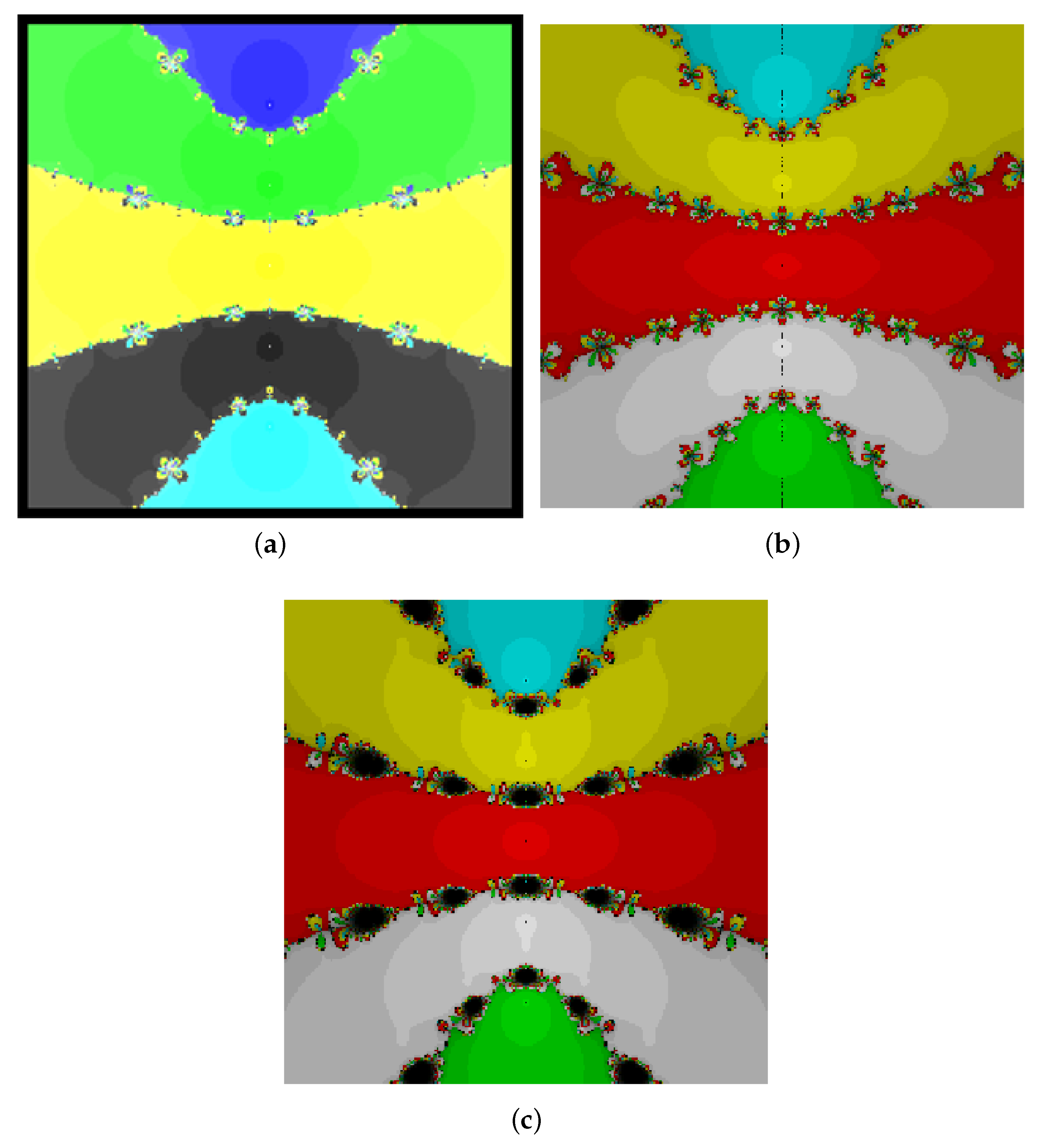
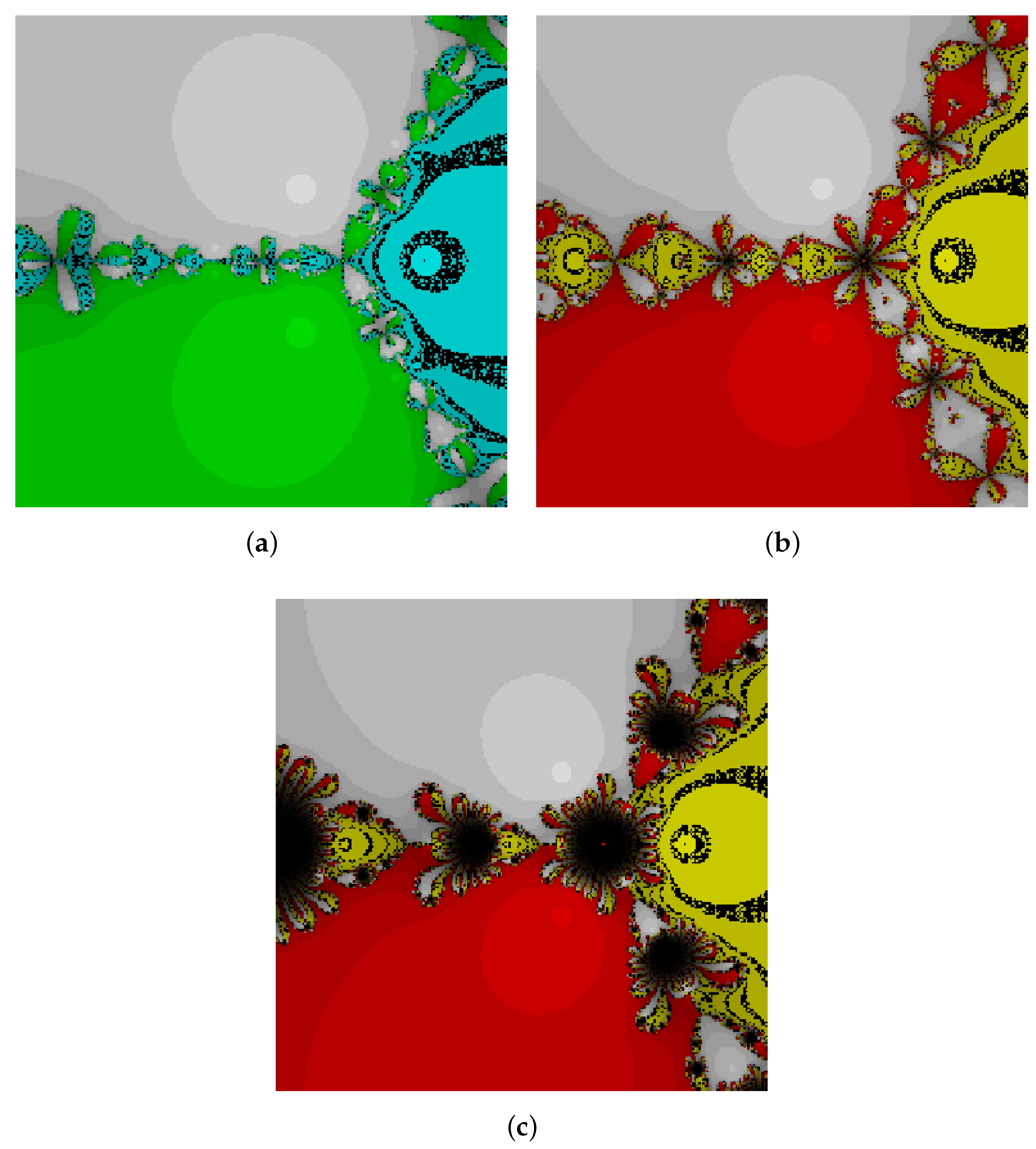
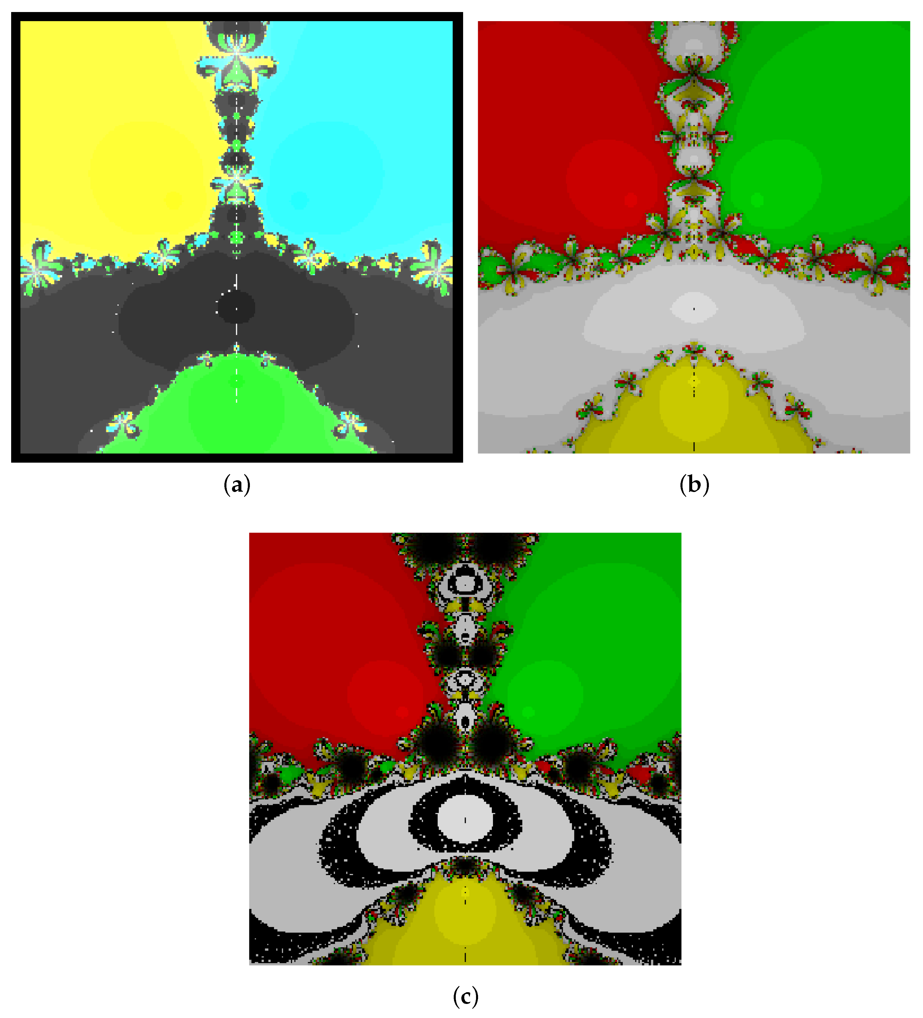
5. Basin of Attraction

The basins of attraction for a function, for a given method, are the sets of initial values from which the iteration will converge to each root. Mathematically, for a given function f defined on the complex plane $\mathbb{C}$, with the roots ${\mathsf{c}}_1,{\mathsf{c}}_2,{\mathsf{c}}_3,{\mathsf{c}}_3,{\mathsf{c}}_5\dots ,{\mathsf{c}}_k\in \mathbb{C}$, then the basin of attraction for the root ${\mathsf{c}}_k$ is

$$B\left({\mathsf{c}}_k\right)=\{\mathsf{c}\in \mathbb{C}\mid theiteration{\gamma }_{n+1}=\mathsf{\Theta }\left({\gamma }_n\right)with{\gamma }_0=\mathsf{c}convergestotheroot{\mathsf{c}}_k\}$$

(47)

If the iterations converge to the root, then the region will be colorful; if the iteration fails to converge, then the region will be black or the color that is not assigned to the basin. One more interesting thing is the “lobes” that occur along the diagonal lines separating the main basins for each root. The region around the root where the iteration will not jump off and converge to the root appears to be the smallest.

The basin of attraction for the complex Newton method was first considered and attributed to Cayley [17,18,19]. It is the fusion of mathematics and art, which shows the beauty of iterative techniques. Understanding the basin of attraction helps the overall behavior and convergence properties of the iterative method. The concept of this section is to use this graphical tool to show the basins of different methods.

In order to view the basins of attraction for complex functions, we make use of an efficient computer programming package, Mathematica 11.3. We consider a rectangle region denoted as $\Omega =[-3,3]\times [-3,3]\subset \mathbb{C}$ in the complex plane. This rectangle is divided into a grid with 450 points on each axis. Using our iterative methods, we begin the process from each initial point $z^{\left(0\right)}$. By taking a maximum of 100 iterations and a tolerance criterion of $|\varphi \left(z^{\left(k\right)}\right)|<{10}^{-4}$, we determine whether $z^{\left(0\right)}$ is the basin of attraction for a specific root or not.

Problem 1.

We chose the function

$$\varphi \left(z\right)=z(z^2+1)(z^2+4)$$

$-2i,2i,-i,i$, and 0 are the five roots of the function. In Figure 1, we focus on a rectangular region in the complex plane. We denote the rectangular area as $\Omega =[-3,3]\times [-3,3]\in \mathbb{C}$. We started the iteration from different points within this rectangular area. Figure 1a represents the basin of attraction of the proposed method (PM); Figure 1b [13] and Figure 1c [14] represent the basins of attraction of existing iterative techniques denoted by the basin of attraction (IS and DS, respectively). In Figure 1a, the five colors represent the five roots. In Figure 1b,c, the five colors represent the five distinct roots, and where the iterations do not converge, the root appears as a black color. We used a convergence criterion of less than ${10}^{-4}$. The Julia set is the colorful patterns and outlines created by the boundaries or edges of the attraction areas. This helps to understand the framework of the iteration technique and gives a comprehensive idea about how they behave and converge to form different attraction regions.

Figure 1. Comparison of basins of attraction. (a) Basin of attraction (PM); (b) basin of attraction (IS); (c) basin of attraction (DS).

Problem 2.

We consider the following function [6]:

$$\varphi \left(z\right)={(z-1)}^3-1$$

The equation $\varphi \left(z\right)=0$ has three zeros $2,0.5+0.866025i$, and $0.5-0.866025i$. In Figure 2, we focus on a rectangular region in the complex plane. We denote the rectangular area as $\Omega =[-3,3]\times [-3,3]\in \mathbb{C}$. We started the iteration from different points within this rectangular area. Figure 2a represents the basin of attraction of the proposed method (PM); Figure 2b,c represent the basins of attraction of existing iterative techniques denoted by the basin of attraction (IS and DS, respectively). In Figure 2a, the three colors represent the three roots, and the black region represents where the iterations do not converge to the root. In Figure 2b,c, the three colors represent the three distinct roots, and where the iterations do not converge, the root appears as a black color. We used a convergence criterion of less than ${10}^{-4}$. The Julia set is the colorful patterns and outlines created by the boundaries or edges of the attraction areas. This helps to understand the framework of the iteration technique and gives a comprehensive idea about how they behave and converge to form different attraction regions.

Figure 2. Comparison of basins of attraction. (a) basin of attraction (PM); (b) basin of attraction (IS); (c) basin of attraction (DS).

Problem 3.

We assumed the following polynomial function of order seven:

$$\varphi \left(z\right)=z^7-1$$

The equation $\varphi \left(z\right)=0$ has seven zeros 1, $-0.22521+0.9749281i$, $0.62349+0.781831i$, $-0.900969+0.433884$, $-0.22521-0.9749281i$, $0.62349-0.781831i$, and $-0.900969-0.433884i$. In Figure 3, we focus on a rectangular region in the complex plane. We denote the rectangular area as $\Omega =[-3,3]\times [-3,3]\subset \mathbb{C}$. We started the iteration from different points within this rectangular area. Figure 3a represents the basin of attraction of the proposed method (PM); Figure 3b,c represents the basins of attraction of existing iterative techniques denoted by the basin of attraction (IS and DS, respectively). In Figure 3, the seven colors represent the seven roots, and the white region represents where the iterations do not converge to the root. In Figure 3b,c, the seven colors represent the seven distinct roots, and where the iterations do not converge, the root appears as a black color. We used a convergence criterion of less than ${10}^{-4}$. The Julia set is the colorful patterns and outlines created by the boundaries or edges of the attraction areas. This helps to understand the framework of the iteration technique and gives a comprehensive idea about how they behave and converge to form different attraction regions.

Figure 3. Comparison of basins of attraction. (a) basin of attraction (PM); (b) basin of attraction (IS); (c) basin of attraction (DS).

Problem 4.

Finally, we chose the following polynomial function with complex constants:

$$\varphi \left(z\right)=(z^3-i)(z+2i)$$

(Ref. [19]) $-i,-2i,-0.866025+0.5i$, and $0.866025+0.5i$ are the four zeros of the function. In Figure 4, we focus on a rectangular region in the complex plane. We denote the rectangular area as $\Omega =[-3,3]\times [-3,3]\subset \mathbb{C}$. We started the iteration from different points within this rectangular area. Figure 4a represents the basin of attraction of the proposed method (PM); Figure 4b,c represent the basins of attraction of existing iterative techniques denoted by the basin of attraction (IS and DS, respectively). In Figure 4a, the four colors represent the four roots. In Figure 4b,c, the four colors represent the four distinct roots, and where the iterations do not converge, the root appears as a black color. We used a convergence criterion of less than ${10}^{-4}$. The Julia set is the colorful patterns and outlines created by the boundaries or edges of the attraction areas. This helps to understand the framework of iteration technique and gives a comprehensive idea about how they behave and converge to form different attraction regions.

Figure 4. Comparison of basins of attraction. (a) basin of attraction (PM); (b) basin of attraction (IS); (c) basin of attraction (DS).

6. Conclusions

This research paper presents a novel sixth-order iterative method with an efficiency index of $1.430969$. We demonstrated the existence and uniqueness of the proposed method through comprehensive convergence analysis and local convergence analysis. The numerical examples provided in this study validate the superior performance of our method as compared to existing techniques of the same order. The basin of attraction figures also illustrate a reduced divergence region with less chaotic behavior as compared to existing techniques of the same order. Finally, we conclude that our methods can be a good alternative to the existing methods.

References

- Solaiman, S.O.; Sihwail, R.; Shehadeh, H.; Hashim, I.; Alieyan, K. Hybrid Newton–Sperm Swarm Optimization Algorithm for Nonlinear Systems. Mathematics 2023, 11, 1473. [Google Scholar] [CrossRef]
- Singh, S.; Gupta, D.K. Iterative methods of higher order for nonlinear equations. Vietnam. J. Math. 2016, 44, 387–398. [Google Scholar] [CrossRef]
- Grau, M.; Díaz-Barrero, J.L. An improvement of the Euler—Chebyshev iterative method. J. Math. Anal. Appl. 2006, 315, 1–7. [Google Scholar] [CrossRef]
- Babajee, D.K.R.; Dauhoo, M.Z.; Darvishi, M.T.; Karami, A.; Barati, A. Analysis of two Chebyshev-like third order methods free from second derivatives for solving systems of nonlinear equations. J. Comput. Appl. Math. 2010, 233, 2002–2012. [Google Scholar] [CrossRef]
- Darvishi, M.T.; Barati, A. A third-order Newton-type method to solve systems of nonlinear equations. Appl. Math. Comput. 2007, 187, 630–635. [Google Scholar] [CrossRef]
- Behl, R.; Maroju, P.; Motsa, S.S. A family of second derivative free fourth order continuation method for solving nonlinear equations. J. Comput. Appl. Math. 2017, 318, 38–46. [Google Scholar] [CrossRef]
- Maheshwari, A.K. A fourth order iterative method for solving nonlinear equations. Appl. Math. Comput. 2009, 211, 383–391. [Google Scholar] [CrossRef]
- Khirallah, M.Q.; Alkhomsan, A.M. A new fifth-order iterative method for solving non-linear equations using weight function technique and the basins of attraction. J. Math. Comput. Sci. 2023, 28, 281–293. [Google Scholar] [CrossRef]
- Abdul-Hassan, N.Y.; Ali, A.H.; Park, C. A new fifth-order iterative method free from second derivative for solving nonlinear equations. J. Appl. Math. Comput. 2022, 68, 2877–2886. [Google Scholar] [CrossRef]
- Cordero, A.; Ezquerro, J.A.; Hernández-Verón, M.A.; Torregrosa, J.R. On the local convergence of a fifth-order iterative method in Banach spaces. Appl. Math. Comput. 2015, 251, 396–403. [Google Scholar] [CrossRef]
- Argyros, I.K.; Khattri, S.K. Local convergence for a family of third order methods in Banach spaces. Punjab Univ. J. Math. 2020, 46, 52–63. [Google Scholar]
- Solaiman, S.O.; Hashim, I. Efficacy of optimal methods for nonlinear equations with chemical engineering applications. Math. Probl. Eng. 2019, 2019, 1728965. [Google Scholar]
- Argyros, I.K.; George, S. Ball convergence of a sixth order iterative method with one parameter for solving equations under weak conditions. Calcolo 2016, 53, 585–595. [Google Scholar] [CrossRef]
- Sharma, D.; Parhi, S.K. On the local convergence of higher order methods in Banach spaces. Fixed Point Theory 2021, 22, 855–870. [Google Scholar] [CrossRef]
- Chapra, S.C. Applied Numerical Methods; McGraw-Hill: Columbus, OH, USA, 2012. [Google Scholar]
- Shih, A.J.; Monteiro, M.C.; Dattila, F.; Pavesi, D.; Philips, M.; da Silva, A.H.; Vos, R.E.; Ojha, K.; Park, S.; van der Heijden, O.; et al. Water electrolysis. Nat. Rev. Methods Prim. 2022, 2, 84. [Google Scholar] [CrossRef]
- Wiersma, A.G. The Complex Dynamics of Newton’s Method. Doctoral Dissertation, Faculty of Science and Engineering, University of Southampton, Southampton, UK, 2016. [Google Scholar]
- Solaiman, O.S.; Karim, S.A.A.; Hashim, I. Dynamical Comparison of Several Third-Order Iterative Methods for Nonlinear Equations. Comput. Mater. Contin. 2021, 67, 1951–1962. [Google Scholar] [CrossRef]
- Sutherland, S. Finding Roots of Complex Polynomials with Newton’s Method. Doctoral Dissertation, Boston University, Boston, MA, USA, 1989. [Google Scholar]
Disclaimer/Publisher’s Note: The statements, opinions and data contained in all publications are solely those of the individual author(s) and contributor(s) and not of MDPI and/or the editor(s). MDPI and/or the editor(s) disclaim responsibility for any injury to people or property resulting from any ideas, methods, instructions or products referred to in the content. |
© 2024 by the authors. Licensee MDPI, Basel, Switzerland. This article is an open access article distributed under the terms and conditions of the Creative Commons Attribution (CC BY) license (https://creativecommons.org/licenses/by/4.0/).