New Order 2.0 Simplified Weak Itô–Taylor Symmetrical Scheme for Stochastic Delay Differential Equations

Abstract

In this article, we construct a new order 2.0 simplified weak Itô–Taylor symmetrical scheme for stochastic delay differential equations. By the new local weak convergence lemma and the connection inequality, we theoretically prove the global weak convergence theorem in two parts on the basis of Malliavin stochastic analysis. Meanwhile, numerical examples are presented to illustrate the error and convergence results. Furthermore, the obtained results display the influence of the delay coefficient on global errors.

1. Introduction

Nowadays, there are many scholars studying differential equations with delay terms.

The authors [1] propose a computationally effective numerical solution for a new design of a second-order Lane–Emden pantograph delayed problem. Stochastic delay differential equations (SDDEs) play a significant role in many application fields, such as control [2], dynamics [3], epidemic problems [4,5] and stock markets [6]. Ain and Wang [7] studied an epidemic model for the evolution of diseases utilizing an Itô–Levy stochastic differential equations system. Among these applications, the application of symmetry principles in the realm of SDDEs offers profound insights into the behavior of complex systems, see [8,9,10]. In this paper, we study d-dimensional SDDEs as follows:

$$\left\{\begin{array}{c}d{X}_t=a(t,X_t,X_{t-\tau \left(t\right)})dt+b(t,X_t,X_{t-\tau \left(t\right)})d{W}_t,t\in [0,T],\hfill \\ X_t=\psi \left(t\right),t\in [-\rho ,0],\hfill \end{array}\right.$$

(1)

where $W_t={(W_t^1,\dots ,W_t^q)}^{\mathbf{T}}$ is q-dimensional normally distributed Brownian motion with mean ${(0,\dots ,0)}^{\mathbf{T}}$ and variance $t{I}_{q\times q}$, and $\psi \left(t\right)$ is a ${\mathcal{F}}_0$-measurable $C([-\rho ,0],{\mathbb{R}}^d)$-valued random variable such that ${sup}_{-\rho \le t\le 0}{\mathbb{E}\left[\right|\psi \left(t\right)|}^2]<\infty .$ Here, the constant $-\rho =inf\{t-\tau (t),t\in [0,T\left]\right\}\le 0,$ and $t-\tau \left(t\right)$ is a continuous increasing function with the variable delay time $\tau \left(t\right).$ The function $a:[0,T]\times {\mathbb{R}}^d\times {\mathbb{R}}^d\to {\mathbb{R}}^d$ is known as the drift coefficient and $b:[0,T]\times {\mathbb{R}}^d\times {\mathbb{R}}^d\to {\mathbb{R}}^{d\times q}$ is the diffusion coefficient.

The existence and uniqueness theorems of SDDEs have been proved by the standard technique of Picard iterations in [11]. Generally, it is difficult to obtain an explicit solution of SDDEs. As a result, many scholars have proposed some numerical schemes for solving SDDEs, such as the Euler–Maruyama scheme [10,12,13,14], $\theta$–Maruyama scheme [15], split-step $\theta$ scheme [16], multistep Maruyama scheme [17] and Runge–Kutta Maruyama scheme [18]. The classical Euler–Maruyama scheme for solving SDEs generally achieves a strong order of convergence $0.5$, and strong convergence schemes have the stability of absolute moments and mean-square stability. In [19,20], the Euler–Maruyama method was employed to solve the stochastic Cahn–Hilliard–Cook equations. Buckwar [8] proposed the strong Euler–Maruyama scheme for Equation (1) and proved the mean-square sense convergence theorem under a global Lipschitz condition by using an induction argument on the interval $[0,T]$. Mao [10,11,21] showed that the Euler–Maruyama numerical solution of SDDEs will converge to the true solution under a local Lipschitz condition by using the technique of stopping times and some moment inequalities for the solution of Equation (1). Subsequently, Mao [22] obtained the convergence in probability of the Euler–Maruyama scheme under a local Lipschitz condition and Khasminskii-type condition.

Given the application requirements in finance and related fields, there is an increasing interest in studying high-order numerical schemes for solving SDEs. Based on the Itô–Taylor expansion, Kolmogorov backward partial differential equations and some weak approximation properties, Kloeden and Platen [23] obtained the weak convergence theorem of classical Itô–Taylor weak high-order schemes for SDEs. However, if the scheme contains multiple stochastic Itô-type integrals, it will consume more CPU time and become computationally inefficient for multidimensional SDEs. In order to improve computational efficiency, the simplified weak second-order method [23] is used to solve multidimensional SDEs, which is highly effective and accurate compared to the classical order 2.0 Itô–Taylor scheme.

In addition, there are also some higher-order numerical schemes for SDDEs. For example, Buckwar and Winkler [17] constructed a linear multistep Maruyama scheme for SDDEs and proved that the implicit two-step backward differentiation method has an order 2.0 convergence rate with the smallest parameter in the noise term. Meanwhile, the weak order 2.0 stochastic orthogonal Runge–Kutta–Chebyshev (S-ROCK) method is proposed in [24,25] for solving SDEs. Then, based on the the S-ROCK method, Guo [18] developed an explicit Runge–Kutta scheme for SDDEs and studied its stability properties.

In this paper, a new order 2.0 simplified weak Itô–Taylor scheme is put forward to solve SDDEs, which is different from the traditional methods in [10,21,23,26]. The primary contributions of this paper can be highlighted as follows:

• A new order 2.0 simplified weak Itô–Taylor symmetrical scheme is proposed for solving SDDEs, which involves no multiple stochastic Itô-type integrals and can be easily applied to solve multidimensional SDDEs.
• Provided that the critical value $\xi =\tau \left(\xi \right)$, we divide the global weak convergence theorem into two steps in the time intervals $[0,\xi ]$ and $(\xi ,T]$. On the basis of the Malliavin space under some reasonable hypotheses, the global weak convergence theorem of the new scheme and the connect inequality are rigorously proven on the time interval $[0,\xi ].$ Subsequently, based on the theory of Malliavin analysis, using the new weak convergence lemmas and the connection inequality between the two intervals $[0,\xi ]$ and $(\xi ,T]$, we rigorously prove that the new scheme has global weak second-order convergence and mean-square stability.
• Several numerical examples, including the Mackey–Glass equation with a multiplicative noise, a nonlinear SDDE about the square of the O-U delay process, a linear SDDE with a time-varying delay and a two-dimensional linear SDDE, are used to illustrate the error and convergence results of the new order 2.0 simplified numerical symmetrical scheme. Additionally, a dedicated discussion section is added to compare our method in detail with other existing methods in terms of computational time and show the global and local convergence rates and mean-square stability property.

The following notations are listed for future reference:

• r is a positive constant, and each line may be different.
• C is a positive constant, and it relies on the upper bounds of the derivatives of the coefficients $a,b,f$.
• $C_b^{i,j,j}:$ the set of functions $U=U(t,x,y):[0,T]\times {\mathbb{R}}^d\times {\mathbb{R}}^d\to \mathbb{R}$ are continuously differentiable with uniformly bounded partial derivatives $\frac{{\partial }^{c}U}{\partial t^c}$ and $\frac{{\partial }^{d+e}U}{\partial x^d\partial y^e}$ for $1\le c\le i$ and $1\le d+e\le j.$
• $C_b^k:$ the set of functions $\varphi :x\in {\mathbb{R}}^d\to \mathbb{R}$ with uniformly bounded partial derivatives $\frac{{\partial }^c\varphi }{\partial x^c}$ for $1\le c\le k.$

This paper is organized as follows. Some fundamental concepts such as the Itô–Taylor expansion and the Malliavin derivative are introduced in Section 2. In Section 3, we present a novel order 2.0 simplified weak Itô–Taylor numerical method for solving stochastic delay differential equations (SDDEs) and prove the global weak convergence theorem. Section 4 provides linear and nonlinear examples to illustrate the impact of the delay coefficient, alongside error and convergence analysis. Finally, in Section 5, we draw our conclusions.

2. Preliminaries

In Section 2.1, we introduce some basic concepts, such as the Itô formula and Itô–Taylor expansion. Further, we list two lemmas and one corollary of the Malliavin derivative in Section 2.2.

2.1. Itô–Taylor Expansion

In this paper, let $(\mathsf{\Omega },\mathcal{F},{\left\{{\mathcal{F}}_t\right\}}_{t\ge 0},P)$ be a complete probability space with the filtration ${\left\{{\mathcal{F}}_t\right\}}_{t\ge 0}$. Furthermore, assume the filtration $\left\{{\mathcal{F}}_t\right\}$ satisfies the usual conditions, i.e., it is right-continuous and ${\mathcal{F}}_0$ contains all P-null sets. Moreover, let the filtration be q-dimensional Brownian motion $W_t$. The random variable $X_t$ is ${\mathcal{F}}_t$-measurable and $\psi \left(t\right)$ is ${\mathcal{F}}_0$-measurable, respectively.

Then, we introduce the set of all multi-indices, which are given by $\mathcal{M}$ in [23]:

$$\mathcal{M}=\{\alpha =(j_1,j_2,\dots ,j_l):j_i\in \{0,1,\dots ,q\},1\le i\le l\mathrm{and}l\ge 1\}\cup \left\{v\right\},$$

where v denotes the empty index. We give the definition of hierarchical set ${\mathsf{\Gamma }}_l$ as follows: ${\mathsf{\Gamma }}_l=\left\{\alpha \in \mathcal{M}:l\left(\alpha \right)\le l\right\},$ and $\mathcal{B}\left({\mathsf{\Gamma }}_l\right)=\left\{\alpha \in \mathcal{M}:l\left(\alpha \right)=l+1\right\}$ denotes the remainder set. Given a multi-index $\alpha \in \mathcal{M}$ with the length $l\left(\alpha \right)>1$, we write $-\alpha =(j_2,\dots ,j_l)$ and $\alpha -=(j_1,j_2,\dots ,j_{l-1})$. Then we have the recursive definition of the multiple Itô integral $I_{\alpha }$ as follows:

$$I_{\alpha }{\left[g_{k,\alpha }(s_1,X_{s_1},X_{s_1-\tau \left(s_1\right)})\right]}_{\rho ,\varsigma }=\left\{\begin{array}{c}{\int }_{\rho }^{\varsigma }{I}_{\alpha -}{\left[g_{k,\alpha }(s_1,X_{s_1},X_{s_1-\tau \left(s_1\right)})\right]}_{\rho ,s_l}d{s}_l,l\ge 1,j_l=0,\hfill \\ {\int }_{\rho }^{\varsigma }{I}_{\alpha -}{\left[g_{k,\alpha }(s_1,X_{s_1},X_{s_1-\tau \left(s_1\right)})\right]}_{\rho ,s_l}d{W}_{s_l}^{j_l},l\ge 1,j_l\ge 1,\hfill \end{array}\right.$$

where $g_{k,\alpha }$ can be represented by

$$g_{k,\alpha }=\left\{\begin{array}{c}{g}_{k,\left(0\right)}=a_k(t,X_t,X_{t-\tau \left(t\right)}),g_{k,\left(i\right)}=b_{k,i}(t,X_t,X_{t-\tau \left(t\right)}),l=1.\hfill \\ L^{j_1}{g}_{k,-\alpha },l>1.\hfill \end{array}\right.$$

For $V\in C^{2,1}([0,T]\times {\mathbb{R}}^d\times {\mathbb{R}}^d;\mathbb{R}),$ we introduce the operators $L^{0}V(t,x,y),$$L^{i}V(t,x,y)$ ($1\le i\le q$) such that

$$\begin{array}{cc}\hfill & L^{0}V(t,x,y)=\frac{\partial }{\partial t}V(t,x,y)+\sum _{k=1}^d\frac{\partial }{\partial x_k}V(t,x,y)a_k(t,x,y)+\frac{1}{2}\sum _{k,l=1}^d\sum _{j=1}^q\frac{{\partial }^2}{\partial x_l\partial x_k}V(t,x,y)b_{k,j}(t,x,y)b_{l,j}(t,x,y),\hfill \\ \hfill & L^{i}V(t,x,y)=\sum _{k=1}^d\frac{\partial }{\partial x_k}V(t,x,y)b_{k,i}(t,x,y),\hfill \end{array}$$

Consequently, by using the above operators, the Itô formula in [21] is presented as

$$V(t,X_t,X_{t-\tau \left(t\right)})=V(0,X_0,X_{-\tau \left(0\right)})+{\int }_0^t{L}^{0}V(s,X_s,X_{s-\tau \left(s\right)})ds+\sum _{i=1}^q{\int }_0^t{L}^{i}V(s,X_s,X_{s-\tau \left(s\right)})d{W}_s^i.$$

Let $X_{k,\varsigma }$ be the k-th component of explicit solution $X_{\varsigma }$ of Equation (1); therefore, we can obtain the following Itô–Taylor expansion:

$$\begin{array}{c}\hfill X_{k,\varsigma }=X_{k,\rho }+\sum _{\alpha \in {\mathsf{\Gamma }}_2\setminus \left\{v\right\}}{g}_{k,\alpha }(\rho ,X_{\rho },X_{\rho -\tau \left(\rho \right)})I_{\alpha }{\left[1\right]}_{\rho ,\varsigma }+\sum _{\alpha \in \mathcal{B}\left({\mathsf{\Gamma }}_2\right)}{I}_{\alpha }{\left[g_{k,\alpha }(s_1,X_{s_1},X_{s_1-\tau \left(s_1\right)})\right]}_{\rho ,\varsigma }.\end{array}$$

2.2. Malliavin Derivative

The Malliavin derivative $D_t$ of a random variable $F={(F_1,\dots ,F_d)}^T$ is given by the following in [27]:

$$D_{t}F={(D_t^{1}F,\dots ,D_t^{q}F)}_{d\times q},D_t^{i}F={(D_t^i{F}_1,\dots ,D_t^i{F}_d)}^T,$$

and

$$D_{t_1\dots t_l}^{\alpha }=D_{t_1\dots t_l}^{(j_1,\dots ,j_l)}=D_{t_1}^{j_1}···D_{t_l}^{j_l}$$

with, especially, $D_{t_k}^0=1$ for $1\le k\le l$.

Furthermore, ${\mathbb{D}}^{k,j}$ can be defined as ordinary Sobolev spaces of functions on ${\mathbb{R}}^d$ that together with their k first partial derivatives have moments of order j with regard to the standard normal law. For any $j\ge 1$ and $k\in \mathbb{N}$, we can define the following norm:

$${\left|\right|G\left|\right|}_{k,j}^j={\mathbb{E}\left[\right|G|}^j]+\sum _{l=1}^k\sum _{\alpha }{\int }_{\rho }^{\varsigma }\dots {\int }_{\rho }^{\varsigma }\mathbb{E}\left[\right|D_{t_1\dots t_l}^{\alpha }G{|}^j]d{t}_1\dots d{t}_l,$$

where G is the smooth random variable. Next, we give two lemmas and a corollary with the Malliavin derivative.

Lemma 1

(duality formula, see [27]). Let $F\in {\mathbb{D}}_{1,2}$ and $X_t\in {\mathbb{D}}_{1,2}$ for $0\le t\le T$. Then for $1\le j\le q$,

$$\begin{array}{cc}\hfill & \mathbb{E}\left[F{\int }_0^T{X}_{t}d{W}_t^j\right]=\mathbb{E}\left[{\int }_0^T{X}_t{D}_t^{j}Fdt\right],D_t^j{\int }_0^T{X}_{s}d{W}_s^j=X_t+{\int }_t^T{D}_t^j{X}_{s}d{W}_s^j.\hfill \end{array}$$

Lemma 2

(chain rules, see [27]). () For $1\le i\le q$, let $G_1,G_2\in {\mathbb{D}}_{1,2}$ and also $G_1{G}_2\in {\mathbb{D}}_{1,2}$ with

$$D_t^i\left(G_1{G}_2\right)=G_1{D}_t^i{G}_2+G_2{D}_t^i{G}_1.$$

Let $G\in {\mathbb{D}}_{1,2}$ and $\varphi \in C^1\left({\mathbb{R}}^d\right)$ with bounded partial derivatives. Then $\varphi \left(G\right)\in {\mathbb{D}}_{1,2}$ and

$$D_t^i\varphi \left(G\right)=\sum _{k=1}^d\frac{\partial }{\partial x_k}\varphi \left(G\right)D_t^i{G}_k.$$

Corollary 1.

For $1\le i,j\le q$, by using the Itô formula, we can obtain the fact that

$${\int }_{\rho }^{\varsigma }{\int }_{\rho }^{t}d{W}_s^{i}d{W}_t^i=\frac{1}{2}\left({(W_{\varsigma }^i-W_{\rho }^i)}^2-(\varsigma -\rho )\right),$$

and we can also deduce the following Malliavin derivative with regard to multiple stochastic integrals:

$$\begin{array}{cc}\hfill & D_r^i({\int }_{\rho }^{\varsigma }{\int }_{\rho }^{t}d{W}_s^{i}d{W}_t^i)=W_{\varsigma }^i-W_{\rho }^i,D_r^i({\int }_{\rho }^{\varsigma }{\int }_{\rho }^{t}d{W}_s^{j}d{W}_t^i)=W_r^j-W_{\rho }^j,\hfill \\ \hfill & D_r^i({\int }_{\rho }^{\varsigma }{\int }_{\rho }^{t}d{W}_s^{i}d{W}_t^j)=W_{\varsigma }^j-W_r^j,D_r^i({\int }_{\rho }^{\varsigma }{\int }_{\rho }^{t}dsd{W}_t^i)=r-\rho \hfill \end{array}$$

for $0\le \rho <r\le \varsigma \le T$ and $i\ne j$.

3. Main Results

In Section 3.1, we present the new order 2.0 simplified weak numerical method for SDDEs on the basis of the Itô–Taylor expansion and trapezoidal rule. Further, by using the new local weak convergence lemma, we obtain the global weak convergence theorems in Section 3.2.

3.1. Order 2.0 Simplified Weak Scheme for SDDEs

Note that the continuous increasing function $t-\tau \left(t\right)\in C[-\rho ,T-\tau (T\left)\right],$ then for $n=0,1,2,\dots ,N$, we first present the uniform partition on time interval $[0,T]$ and $\mathsf{\Delta }t:=\frac{T}{N_0}$, $u_i=i\mathsf{\Delta }t$$(1\le i\le N_0),$ and we define $L:=min\left\{i\right|i\in {\mathbb{N}}^{+},u_i-\tau \left(u_i\right)\ge 0\}$ and $m:=max\left\{i\right|i\in \mathbb{N},i\ge L,u_i-\tau \left(u_i\right)\le u_L\}.$ In this paper, we use the time discretization $\{t_n,0\le n\le N:=2N_0-L+1\}$:

$$0=t_0<\dots <u_m-\tau \left(u_m\right)<\dots \le t_{m+1}=u_L<\dots <t_N=T$$

with step size $\mathsf{\Delta }{t}_n=t_{n+1}-t_n\le \mathsf{\Delta }t$, including all the times $\{u_i,1\le i\le N_0\}$ and $\{u_L-\tau \left(u_L\right),u_{L+1}-\tau \left(u_{L+1}\right),\dots ,u_{N_0}-\tau \left(u_{N_0}\right)\}.$ Then, we have the k-th component of explicit solution $X_{t_{n+1}}$ of Equation (1) by the Itô–Taylor expansion

$$X_{k,t_{n+1}}=X_{k,t_n}+\sum _{\alpha \in {\mathsf{\Gamma }}_2\setminus \left\{v\right\}}{g}_{k,\alpha }(t_n,X_{t_n},X_{t_n-\tau \left(t_n\right)})I_{\alpha }{\left[1\right]}_{t_n,t_{n+1}}+\sum _{\alpha \in \mathcal{B}\left({\mathsf{\Gamma }}_2\right)}{I}_{\alpha }{\left[g_{k,\alpha }(s_1,X_{s_1},X_{s_1-\tau \left(s_1\right)})\right]}_{t_n,t_{n+1}}.$$

(2)

Scheme 1.

For $1\le n\le N-1$ and initial value $X^0=X_0$, it takes the form

$$X_k^{n+1}=X_k^n+a_k\mathsf{\Delta }{t}_n+\sum _{i=1}^q{b}_{k,i}\mathsf{\Delta }{W}_n^i+\frac{1}{2}{L}^0{a}_k{\left(\mathsf{\Delta }{t}_n\right)}^2+\sum _{i=1}^q\frac{1}{2}(L^i{a}_k+L^0{b}_{k,i})\mathsf{\Delta }{W}_n^i\mathsf{\Delta }{t}_n+\sum _{i,j=1}^q\frac{1}{2}{L}^i{b}_{k,j}(\mathsf{\Delta }{W}_n^i\mathsf{\Delta }{W}_n^j+V_{i,j}),$$

where $\mathsf{\Delta }{W}_n^i=W_{t_{n+1}}^i-W_{t_n}^i$, $a_k=a_k(t_n,X^n,X^{n-m})$ and $b_{k,i}=b_{k,i}(t_n,X^n,X^{n-m}),$ and

$$X^{n-m}=\left\{\begin{array}{c}\psi (t_n-\tau \left(t_n\right)),0\le n\le m,\hfill \\ X^{n-m},m<n\le N,\hfill \end{array}\right.$$

where the $V_{i,j}$ are independent two-point distributed random variables with $P(V_{i,j}=\pm \mathsf{\Delta }{t}_n)=\frac{1}{2}$ for $j=1,\dots ,i-1$, $V_{i,i}=-\mathsf{\Delta }t$ and $V_{i,j}=-V_{j,i}$ for $i=1,\dots ,q$ and $j=i+1,\dots ,q$.

Hypothesis 1.

Assume the functions $a,b$ satisfy the following conditions:

• Lipschitz condition: for $x_1,x_2,y_1,y_2\in {\mathbb{R}}^d,t\in [0,T]$, there is a constant $L>0$ with

  $$\begin{array}{c}\hfill |a(t,x_1,y_1)-a(t,x_2,y_2)|\vee |b(t,x_1,y_1)-b(t,x_2,y_2)|\le L(|x_1-x_2|+|y_1-y_2\left|\right).\end{array}$$
• Linear growth condition: for $x,y\in {\mathbb{R}}^d,$ there is a positive constant K with

  $$\begin{array}{c}\hfill {\left|a(t,x,y)\right|}^2\vee {\left|b(t,x,y)\right|}^2\le {K(1+|x|}^2+{\left|y\right|}^2).\end{array}$$

At the same time, the functions ψ satisfy the following conditions:

• The Hölder continuity of the initial data: for all $-\rho \le s<t\le 0$, there exist constants $H>0$ and $\gamma \in \left(0,1\right]$ such that

  $$\begin{array}{c}\hfill {\mathbb{E}\left[\right|\psi \left(t\right)-\psi \left(s\right)|}^2{]\le H(|t-s|}^{\gamma }).\end{array}$$

Let $X_t$ and $X^n$ be the solution of Equation (1) and Scheme 1, respectively. We have the following hypothesis.

Hypothesis 2.

Assume the functions $a,b\in C_b^{2,3,3}$, $\psi \in C_b^3$.

Lemma 3.

$X_t$ and $X^n$$(0\le n\le N)$ are the solutions of Equation (1) and Scheme 1, respectively. Under Hypotheses 1 and 2, we can obtain ${\left\{X_t\right\}}_{0\le t\le T}\in {\mathbb{D}}^{3,2}$ and ${\left\{X^n\right\}}_{0\le n\le N}\in {\mathbb{D}}^{3,2}$.

Proof. 

Assume $X_t$ is the explicit solution of following equation:

$$X_t=X_0+{\int }_0^{t}a(s,X_s,X_{s-\tau \left(s\right)})ds+{\int }_0^{t}b(s,X_s,X_{s-\tau \left(s\right)})d{W}_s.$$

(3)

Using the B-D-G inequality, Gronwall’s inequality and Hypothesis 1, one can show that in reference [11],

$$\mathbb{E}[\underset{0\le r\le t}{sup}|X_r{|}^2]\le (1+3\mathbb{E}[|X_0{|}^2\left]\right)e^{3KT(T+4)}.$$

(4)

By taking the Malliavin derivative with respect to Equation (3), we obtain

$$D_r{X}_t={\int }_r^t{D}_{r}a(s,X_s,X_{s-\tau \left(s\right)})ds+b(r,X_r,X_{r-\tau \left(r\right)})+{\int }_r^t{D}_{r}b(s,X_s,X_{s-\tau \left(s\right)})d{W}_s,$$

(5)

where $0\le r\le t\le T$ and

$$D_{r}a(s,X_s,X_{s-\tau \left(s\right)})=a_2^{\prime }(s,X_s,X_{s-\tau \left(s\right)})D_r{X}_s+a_3^{\prime }(s,X_s,X_{s-\tau \left(s\right)})D_r{X}_{s-\tau \left(s\right)},$$

$$D_{r}b(s,X_s,X_{s-\tau \left(s\right)})=b_2^{\prime }(s,X_s,X_{s-\tau \left(s\right)})D_r{X}_s+b_3^{\prime }(s,X_s,X_{s-\tau \left(s\right)})D_r{X}_{s-\tau \left(s\right)}.$$

Using the elementary inequality ${({\displaystyle \sum _{i=1}^3}{c}_i)}^2\le 3{\displaystyle \sum _{i=1}^3}{c}_i^2$ and $a,b\in C_b^{·,1,1}$, one can further show that

$${(D_r{X}_t)}^2\le 3{(b(r,X_r,X_{r-\tau (r)}))}^2+3T{\int }_r^t{(D_{r}a(s,X_s,X_{s-\tau (s)}))}^{2}ds+3{({\int }_r^t{D}_{r}b(s,X_s,X_{s-\tau (s)})d{W}_s)}^2.$$

(6)

Then using Hölder’s inequality, we have

$$\begin{array}{cc}\hfill \mathbb{E}[|D_r{X}_t{|}^2]& \le 3\mathbb{E}[|b(r,X_r,X_{r-\tau \left(r\right)}){|}^2]+3T{\int }_r^T\mathbb{E}[|D_{r}a(s,X_s,X_{s-\tau \left(s\right)}){|}^2]ds+3{\int }_r^T\mathbb{E}[|D_{r}b(s,X_s,X_{s-\tau \left(s\right)}){|}^2]ds\hfill \\ \hfill & \le C\underset{0\le s\le T}{sup}\mathbb{E}\left[1+|X_s{|}^2+{|X_{s-\tau \left(s\right)}|}^2\right]+CT{\int }_r^T\mathbb{E}[|D_r{X}_s{|}^2]ds,\hfill \end{array}$$

which by the Gronwall inequality yields

$$\mathbb{E}[|D_r{X}_t{|}^2]\le C\underset{0\le s\le T}{sup}\mathbb{E}\left[1+|X_s{|}^2+{|X_{s-\tau \left(s\right)}|}^2\right]e^{CT}\le C.$$

(7)

Further, if $a,b\in C_b^{2,4,4}$, $\psi \in C_b^4,$ we obtain that

$$\mathbb{E}[|D_{s_1}{D}_{s_2}{X}_t{|}^2]\le C,\mathbb{E}[|D_{s_1}{D}_{s_2}{D}_{s_3}{X}_t{|}^2]\le C,$$

(8)

which yields ${\left\{X_t\right\}}_{0\le t\le T}\in {\mathbb{D}}^{3,2}$. Applying similar techniques as in the proofs of Inequalities (4) and (7), under the conditions of the lemma, we deduce ${\left\{X^n\right\}}_{0\le n\le N}\in {\mathbb{D}}^{3,2}$. □

3.2. Weak Convergence Theorems

For the sake of a simple proof, we present a new local weak convergence lemma before presenting the proof of global weak convergence. Next, we give two theorems to prove the global weak convergence theory on the basis of the new weak convergence lemma. In Theorem 1, we utilize the theory of Malliavin analysis and the new lemma to prove Scheme 1 has the global weak second-order convergence rate within $[0,t_m]$. Based on Theorem 1, we prove the global weak convergence theorem within $[t_m,T]$ in Theorem 2.

Lemma 4

(Local weak convergence). Let $X_{t_{n+1}}$ and $X^{n+1}$$(0\le n\le N-1)$ be the solutions of Equation (1) and Scheme 1, respectively. Assume $F^{n+1}=F(X_{t_{n+1}},X^{n+1}):{\mathbb{R}}^d\times {\mathbb{R}}^d\to \mathbb{R}$. Under Hypothesis 1 and Hypothesis 2, for $1\le j\le q,$ we have

$$|\mathbb{E}\left[F(X_{t_{n+1}},X^{n+1})\left({\int }_{t_n}^{t_{n+1}}{\int }_{t_n}^{t}d{W}_s^{j}dt-\frac{1}{2}\mathsf{\Delta }{W}_n^j\mathsf{\Delta }{t}_n\right)\right]|\le C(1+\mathbb{E}[|X_0{|}^r]){(\mathsf{\Delta }t)}^3$$

(9)

and

$$|\mathbb{E}\left[F(X_{t_{n+1}},X^{n+1})\left({\int }_{t_n}^{t_{n+1}}{\int }_{t_n}^{t}dsd{W}_t^j-\frac{1}{2}\mathsf{\Delta }{t}_n\mathsf{\Delta }{W}_n^j\right)\right]|\le C(1+\mathbb{E}[|X_0{|}^r]){(\mathsf{\Delta }t)}^3.$$

(10)

Proof. 

For $1\le j\le q$, by taking the Malliavin derivative on both sides of Scheme 1 and Equation (2), we can obtain

$$\begin{array}{cc}\hfill & D_s^j{X}_k^{n+1}=b_{k,j}+\frac{1}{2}{L}^j{a}_k\mathsf{\Delta }{t}_n+\frac{1}{2}{L}^0{b}_{k,j}\mathsf{\Delta }{t}_n+L^j{b}_{k,j}\mathsf{\Delta }{W}_n^j+\frac{1}{2}\sum _{i=1,i\ne j}^q(L^j{b}_{k,i}+L^i{b}_{k,j})\mathsf{\Delta }{W}_n^i,\hfill \end{array}$$

(11)

$$\begin{array}{cc}\hfill & D_s^j{X}_{k,t_{n+1}}=\sum _{\alpha \in {\mathsf{\Gamma }}_2\setminus \left\{v\right\}}{g}_{k,\alpha }(t_n,X_{t_n},X_{t_n-\tau \left(t_n\right)})D_s^j{I}_{\alpha }{\left[1\right]}_{t_n,t_{n+1}}+\sum _{\alpha \in \mathcal{B}\left({\mathsf{\Gamma }}_2\right)}{D}_s^j{I}_{\alpha }{\left[g_{k,\alpha }(s_1,X_{s_1},X_{s_1-\tau \left(s_1\right)})\right]}_{t_n,t_{n+1}}\hfill \end{array}$$

(12)

for $t_n<s\le t_{n+1}$. Using Lemma 1 (duality formula), we conclude that

$$\begin{array}{cc}& \mathbb{E}\left[F(X_{t_{n+1}},X^{n+1})\left({\int }_{t_n}^{t_{n+1}}{\int }_{t_n}^{t}d{W}_s^{j}dt-\frac{1}{2}\mathsf{\Delta }{W}_n^j\mathsf{\Delta }{t}_n\right)\right]\hfill \\ \hfill =& \mathbb{E}\left[{\int }_{t_n}^{t_{n+1}}{\int }_{t_n}^t{D}_s^j\left(F(X_{t_{n+1}},X^{n+1})\right)dsdt-\frac{1}{2}{\int }_{t_n}^{t_{n+1}}{\int }_{t_n}^{t_{n+1}}{D}_s^j\left(F(X_{t_{n+1}},X^{n+1})\right)dsdt\right].\hfill \end{array}$$

(13)

Combining Equations (11) and (12) and Corollary 1, for $t_n<s\le t_{n+1}$, we have

$$D_s^j\left(F(X_{t_{n+1}},X^{n+1})\right)=F_1^{\prime }(X_{t_{n+1}},X^{n+1})D_s^j{X}_{t_{n+1}}+F_2^{\prime }(X_{t_{n+1}},X^{n+1})D_s^j{X}^{n+1}={\varphi }_1+{\varphi }_{2,s}.$$

(14)

Here, ${\varphi }_1:={\varphi }_1(t_n,X^n,X^{n-m},X_{t_{n+1}},X^{n+1},\mathsf{\Delta }{W}_n,\mathsf{\Delta }{t}_n)$ is a function not depending only on time s, and

$$\begin{array}{cc}\hfill & {\varphi }_{2,s}:=(W_{t_{n+1}}-W_s)G_1^{n+1}+(W_s-W_{t_n})G_2^{n+1}+G_3^{n+1},\hfill \end{array}$$

(15)

where

$$\begin{array}{cc}\hfill & G_1^{n+1}:=G_1^{n+1}(X^n,X_{t_n},X^{n+1},X_{t_{n+1}}),G_2^{n+1}:=G_2^{n+1}(X^n,X_{t_n},X^{n+1},X_{t_{n+1}}),\hfill \\ \hfill & G_3^{n+1}:=G_3^{n+1}(\mathsf{\Delta }{t}_n,X^n,X^{n-m},X_{t_{n+1}},X^{n+1},s-t_n,t_{n+1}-s)\hfill \end{array}$$

(16)

with the property

$$|\mathbb{E}\left[G_3^{n+1}(\mathsf{\Delta }{t}_n,X^n,X^{n-m},X_{t_{n+1}},X^{n+1},s-t_n,t_{n+1}-s)\right]|\le C(1+\mathbb{E}[|X_0{|}^r\left]\right)\mathsf{\Delta }t.$$

(17)

On the basis of Equations (13) and (14), we immediately obtain that

$$\begin{array}{cc}& \mathbb{E}\left[F(X_{t_{n+1}},X^{n+1})\left({\int }_{t_n}^{t_{n+1}}{\int }_{t_n}^{t}d{W}_s^{j}dt-\frac{1}{2}\mathsf{\Delta }{W}_n^j\mathsf{\Delta }{t}_n\right)\right]\hfill \\ \hfill =& \mathbb{E}\left[{\int }_{t_n}^{t_{n+1}}{\int }_{t_n}^t({\varphi }_1+{\varphi }_{2,s})dsdt-\frac{1}{2}{\int }_{t_n}^{t_{n+1}}{\int }_{t_n}^{t_{n+1}}({\varphi }_1+{\varphi }_{2,s})dsdt\right]\hfill \\ \hfill =& {\epsilon }_1+{\epsilon }_2,\hfill \end{array}$$

(18)

where

$$\begin{array}{cc}\hfill & {\epsilon }_1=\mathbb{E}\left[{\varphi }_1\right]\left({\int }_{t_n}^{t_{n+1}}{\int }_{t_n}^{t}dsdt-\frac{1}{2}{\int }_{t_n}^{t_{n+1}}{\int }_{t_n}^{t_{n+1}}dsdt\right),\hfill \\ \hfill & {\epsilon }_2=\mathbb{E}\left[{\int }_{t_n}^{t_{n+1}}{\int }_{t_n}^t{\varphi }_{2,s}dsdt-\frac{1}{2}{\int }_{t_n}^{t_{n+1}}{\int }_{t_n}^{t_{n+1}}{\varphi }_{2,s}dsdt\right].\hfill \end{array}$$

Since ${\int }_{t_n}^{t_{n+1}}{\int }_{t_n}^{t}dsdt-\frac{1}{2}{\int }_{t_n}^{t_{n+1}}{\int }_{t_n}^{t_{n+1}}dsdt=0,$ we have ${\epsilon }_1=0$. Using Lemma 1 (duality formula), it follows from Equations (15) and (16) that

$$\mathbb{E}\left[(W_{t_{n+1}}-W_s)G_1^{n+1}\right]={\int }_s^{t_{n+1}}\mathbb{E}\left[D_r{G}_1^{n+1}\right]dr,\mathbb{E}\left[(W_s-W_{t_n})G_2^{n+1}\right]={\int }_{t_n}^s\mathbb{E}\left[D_r{G}_2^{n+1}\right]dr$$

(19)

for $t_n<s\le t_{n+1}.$ Utilizing Equations (15), (17) and (19), we deduce

$$|{\epsilon }_2|=|\mathbb{E}\left[{\int }_{t_n}^{t_{n+1}}{\int }_{t_n}^t{\varphi }_{2,s}dsdt-\frac{1}{2}{\int }_{t_n}^{t_{n+1}}{\int }_{t_n}^{t_{n+1}}{\varphi }_{2,s}dsdt\right]|\le C(1+\mathbb{E}[|X_0{|}^r\left]\right){\left(\mathsf{\Delta }t\right)}^3.$$

(20)

Consequently, from the fact ${\epsilon }_1=0$, by Equations (18) and (20), we obtain

$$|\mathbb{E}\left[F(X_{t_{n+1}},X^{n+1})\left({\int }_{t_n}^{t_{n+1}}{\int }_{t_n}^{t}d{W}_s^{j}dt-\frac{1}{2}\mathsf{\Delta }{W}_n^j\mathsf{\Delta }{t}_n\right)\right]|\le C(1+\mathbb{E}[|X_0{|}^r\left]\right){\left(\mathsf{\Delta }t\right)}^3.$$

Applying similar techniques as those used to prove Inequality (9), we obtain that Inequality (10) holds.

The proof is completed. □

For the ease of the proof, we consider one-dimensional Wiener process $W_t$ and random variable $X_t$. Next, we give the proof of global weak convergence (Theorem 1) on $t\in [0,t_m]$.

Theorem 1

(global weak convergence: part I). Let Hypotheses 1 and 2 hold. Let $X_t$ and $X^n$ ($1\le n\le m$) be the solutions of Equation (1) and Scheme 1, respectively. Then, if $f\in C_b^4,$ $U^n\in {\mathbb{D}}^{3,2}$ ($1\le n\le m$), we have

$$\begin{array}{cc}\hfill & \mathrm{w}\mathrm{e}\mathrm{a}\mathrm{k} \mathrm{c}\mathrm{o}\mathrm{n}\mathrm{v}\mathrm{e}\mathrm{r}\mathrm{g}\mathrm{e}\mathrm{n}\mathrm{c}\mathrm{e} \mathrm{i}\mathrm{n}\mathrm{e}\mathrm{q}\mathrm{u}\mathrm{a}\mathrm{l}\mathrm{i}\mathrm{t}\mathrm{y}:|\mathbb{E}[f\left(X_{t_m}\right)-f\left(X^m\right)]|\le C(1+\mathbb{E}[|X_0{|}^r\left]\right){\left(\mathsf{\Delta }t\right)}^2;\hfill \end{array}$$

(21)

$$\begin{array}{cc}\hfill & \mathrm{c}\mathrm{o}\mathrm{n}\mathrm{n}\mathrm{e}\mathrm{c}\mathrm{t}\mathrm{i}\mathrm{o}\mathrm{n} \mathrm{i}\mathrm{n}\mathrm{e}\mathrm{q}\mathrm{u}\mathrm{a}\mathrm{l}\mathrm{i}\mathrm{t}\mathrm{y}:|\mathbb{E}\left[(X_{t_n}-X^n)U^n\right]|\le C(1+\mathbb{E}[|X_0{|}^r\left]\right){\left(\mathsf{\Delta }t\right)}^2.\hfill \end{array}$$

(22)

Proof. 

In the case that the time $t_{m+1}=u_L$, it follows from the Taylor formula that

$$f\left(X_{t_m}\right)-f\left(X^m\right)=(X_{t_m}-X^m)f_{\lambda }^m$$

(23)

with $f_{\lambda }^m={\int }_0^1\frac{d}{dx}f(X^m+\lambda (X_{t_m}-X^m))d\lambda .$ Note that

$${\int }_{t_{m-1}}^{t_m}{\int }_{t_{m-1}}^{s_2}d{W}_{s_1}d{W}_{s_2}=\frac{1}{2}\left({\left(\mathsf{\Delta }{W}_{m-1}\right)}^2-\mathsf{\Delta }{t}_{m-1}\right)\mathrm{and}{\int }_{t_{m-1}}^{t_m}{\int }_{t_{m-1}}^{s_2}d{s}_{1}d{s}_2=\frac{1}{2}{\left(\mathsf{\Delta }{t}_{m-1}\right)}^2,$$

so by virtue of the Itô–Taylor expansion, we can obtain

$$\begin{array}{cc}\hfill X_{t_m}-X^m& =X_{t_{m-1}}-X^{m-1}+\sum _{\alpha \in \mathcal{B}\left({\mathsf{\Gamma }}_2\right)}{I}_{\alpha }{\left[g_{\alpha }(s_1,X_{s_1},\psi (s_1-\tau \left(s_1\right)))\right]}_{t_{m-1},t_m}\hfill \\ \hfill & +\sum _{\alpha \in {\mathsf{\Gamma }}_2\setminus \left\{v\right\}}\left(g_{\alpha }(t_{m-1},X_{t_{m-1}},\psi (t_{m-1}-\tau \left(t_{m-1}\right)))-g_{\alpha }(t_{m-1},X^{m-1},\psi (t_{m-1}-\tau \left(t_{m-1}\right)))\right)I_{\alpha }{\left[1\right]}_{t_{m-1},t_m}\hfill \\ \hfill & +\sum _{j_1\ne j_2}{g}_{\alpha }(t_{m-1},X^{m-1},\psi (t_{m-1}-\tau \left(t_{m-1}\right)))\left({\int }_{t_{m-1}}^{t_m}{\int }_{t_{m-1}}^{s_2}d{W}_{s_1}^{j_1}d{W}_{s_2}^{j_2}-\frac{1}{2}\mathsf{\Delta }{W}_{m-1}^{j_1}\mathsf{\Delta }{W}_{m-1}^{j_2}\right)\hfill \end{array}$$

(24)

for $1\le j_1,j_2\le q$ and $W_s^0=s.$ For $g_{\alpha }=g_{\alpha }(t,x,y)$, it follows from the Taylor formula that

$$g_{\alpha }(t_{m-1},X_{t_{m-1}},\psi (t_{m-1}-\tau \left(t_{m-1}\right)))-g_{\alpha }(t_{m-1},X^{m-1},\psi (t_{m-1}-\tau \left(t_{m-1}\right)))=(X_{t_{m-1}}-X^{m-1})G_{\alpha ,x,\psi }^{m-1},$$

(25)

where $G_{\alpha ,x,\psi }^{m-1}={\int }_0^1\frac{\partial }{\partial x}{g}_{\alpha }(t_{m-1},X^{m-1}+\lambda (X_{t_{m-1}}-X^{m-1}),\psi (t_{m-1}-\tau ))d\lambda$. Combining Equations (23)–(25), we have

$$\begin{array}{cc}\hfill & \mathbb{E}\left[f\left(X_{t_m}\right)-f\left(X^m\right)\right]=\mathbb{E}\left[(X_{t_m}-X^m)f_{\lambda }^m\right]\hfill \\ \hfill & =\mathbb{E}\left[(X_{t_{m-1}}-X^{m-1})\left(f_{\lambda }^m+\sum _{\alpha \in {\mathsf{\Gamma }}_2\setminus \left\{v\right\}}{G}_{\alpha ,x,\psi }^{m-1}{f}_{\lambda }^m{I}_{\alpha }{\left[1\right]}_{t_{m-1},t_m}\right)\right]+{\mathcal{E}}_1^{m-1}+{\mathcal{E}}_2^{m-1}\hfill \\ \hfill & =\mathbb{E}\left[(X_{t_{m-1}}-X^{m-1})F^{m-1}\right]+\sum _{j=1}^2{\mathcal{E}}_j^{m-1},\hfill \end{array}$$

(26)

where

$$\begin{array}{cc}\hfill & F^{m-1}:=f_{\lambda }^m\left(1+\sum _{\alpha \in {\mathsf{\Gamma }}_2\setminus \left\{v\right\}}{G}_{\alpha ,x,\psi }^{m-1}{I}_{\alpha }{\left[1\right]}_{t_{m-1},t_m}\right),\hfill \end{array}$$

(27)

$$\begin{array}{cc}\hfill & {\mathcal{E}}_1^{m-1}:=\sum _{j_1\ne j_2}\mathbb{E}\left[g_{\alpha }\left(t_{m-1},X^{m-1},\psi (t_{m-1}-\tau \left(t_{m-1}\right))\right)f_{\lambda }^m\left({\int }_{t_{m-1}}^{t_m}{\int }_{t_{m-1}}^{s_2}d{W}_{s_1}^{j_1}d{W}_{s_2}^{j_2}-\frac{1}{2}\mathsf{\Delta }{W}_{m-1}^{j_1}\mathsf{\Delta }{W}_{m-1}^{j_2}\right)\right],\hfill \end{array}$$

(28)

$$\begin{array}{cc}\hfill & {\mathcal{E}}_2^{m-1}:=\sum _{\alpha \in \mathcal{B}\left({\mathsf{\Gamma }}_2\right)}\mathbb{E}\left[f_{\lambda }^m{I}_{\alpha }{\left[g_{\alpha }(s_1,X_{s_1},\psi (s_1-\tau \left(s_1\right)))\right]}_{t_{m-1},t_m}\right].\hfill \end{array}$$

(29)

From Equation (26), we deduce the following recursive formula:

$$\mathbb{E}\left[f\left(X_{t_m}\right)-f\left(X^m\right)\right]=\mathbb{E}\left[(X_{t_{m-1}}-X^{m-1})F^{m-1}\right]+\sum _{j=1}^2{\mathcal{E}}_j^{m-1}=\mathbb{E}\left[(X_{t_1}-X^1)F^1\right]+\sum _{l=1}^{m-1}\sum _{j=1}^2{\mathcal{E}}_j^l,$$

(30)

where $F^{m-1},{\mathcal{E}}_1^{m-1}$ and ${\mathcal{E}}_2^{m-1}$ are defined in (27), (28) and (29), respectively, and for $1\le i\le m-2,$

$$\begin{array}{cc}\hfill & F^i:=F^{i+1}\left(1+\sum _{\alpha \in {\mathsf{\Gamma }}_2\setminus \left\{v\right\}}{G}_{\alpha ,x,\psi }^i{I}_{\alpha }{\left[1\right]}_{t_i,t_{i+1}}\right),\hfill \end{array}$$

(31)

$$\begin{array}{cc}\hfill & {\mathcal{E}}_1^i:=\sum _{j_1\ne j_2}\mathbb{E}\left[g_{\alpha }\left(t_i,X^i,\psi (t_i-\tau \left(t_i\right))\right)F^{i+1}\left({\int }_{t_i}^{t_{i+1}}{\int }_{t_i}^{s_2}d{W}_{s_1}^{j_1}d{W}_{s_2}^{j_2}-\frac{1}{2}\mathsf{\Delta }{W}_i^{j_1}\mathsf{\Delta }{W}_i^{j_2}\right)\right],\hfill \\ \hfill & {\mathcal{E}}_2^i:=\sum _{\alpha \in \mathcal{B}\left({\mathsf{\Gamma }}_2\right)}\mathbb{E}\left[F^{i+1}{I}_{\alpha }{\left[g_{\alpha }(s_1,X_{s_1},\psi (s_1-\tau \left(s_1\right)))\right]}_{t_i,t_{i+1}}\right].\hfill \end{array}$$

In order to give the estimate with respect to Equation (30), we give the detailed proof process in three parts. In the first part, let the condition $X_0=X^0$, so we obtain

$$X_{t_1}-X^1=\sum _{\alpha \in \mathcal{B}\left({\mathsf{\Gamma }}_2\right)}{I}_{\alpha }[g_{\alpha }\left(s_1,X_{s_1},\psi (s_1-\tau \left(s_1\right))\right){]}_{t_0,t_1}.$$

(32)

Using Lemma 1 (duality formula) and Equation (32), it yields

$$\begin{array}{cc}\hfill \mathbb{E}\left[(X_{t_1}-X^1)F^1\right]& =\sum _{\alpha \in \mathcal{B}\left({\mathsf{\Gamma }}_2\right)}\mathbb{E}\left[F^1{I}_{\alpha }{\left[g_{\alpha }(s_1,X_{s_1},\psi (s_1-\tau \left(s_1\right)))\right]}_{t_0,t_1}\right]\hfill \\ \hfill & =\sum _{\alpha \in \mathcal{B}\left({\mathsf{\Gamma }}_2\right)}{I}_{(0,0,0)}{\left[\mathbb{E}\left[D_{s_1{s}_2{s}_3}^{\alpha }\left(F^1\right)g_{\alpha }(s_1,X_{s_1},\psi (s_1-\tau \left(s_1\right)))\right]\right]}_{t_0,t_1}.\hfill \end{array}$$

(33)

It follows from the condition in Hypotheses 1 and 2 that $G_{\alpha ,x,\psi }^i=G_{\alpha ,x,\psi }^i(X_{t_i},X^i)\in {\mathbb{D}}^{3,2}$ for $1\le i\le m-1$ and $f_{\lambda }^m=f_{\lambda }^m(X_{t_m},X^m)\in {\mathbb{D}}^{3,2},$ which, by combining the Equations (27) and (31), yields

$$F^1=f_{\lambda }^m\prod _{i=1}^{m-1}\left(1+\sum _{\alpha \in {\mathsf{\Gamma }}_2\setminus \left\{v\right\}}{G}_{\alpha ,x,\psi }^i{I}_{\alpha }{\left[1\right]}_{t_i,t_{i+1}}\right)\in {\mathbb{D}}^{3,2}.$$

(34)

Consequently, we can infer from (33) and (34) that

$$|\mathbb{E}\left[(X_{t_1}-X^1)F^1\right]|\le C(1+\mathbb{E}[|X_0{|}^r\left]\right){\left(\mathsf{\Delta }t\right)}^3.$$

(35)

In the second part, we give the error estimate with respect to ${\mathcal{E}}_1^i$:

$$\begin{array}{cc}\hfill {\mathcal{E}}_1^i& =\sum _{j_1\ne j_2}\mathbb{E}\left[g_{\alpha }(t_i,X^i,\psi (t_i-\tau \left(t_i\right)))F^{i+1}\left({\int }_{t_i}^{t_{i+1}}{\int }_{t_i}^{s_2}d{W}_{s_1}^{j_1}d{W}_{s_2}^{j_2}-\frac{1}{2}\mathsf{\Delta }{W}_i^{j_1}\mathsf{\Delta }{W}_i^{j_2}\right)\right]\hfill \\ \hfill & =\sum _{j_1\ne j_2}\mathbb{E}\left[g_{\alpha }(t_i,X^i,\psi (t_i-\tau \left(t_i\right)))\mathbb{E}\left[F^{i+1}\left({\int }_{t_i}^{t_{i+1}}{\int }_{t_i}^{s_2}d{W}_{s_1}^{j_1}d{W}_{s_2}^{j_2}-\frac{1}{2}\mathsf{\Delta }{W}_i^{j_1}\mathsf{\Delta }{W}_i^{j_2}\right)|{\mathcal{F}}_{t_i}\right]\right].\hfill \end{array}$$

Next, by using Lemma 4, we have $|{\mathcal{E}}_1^i|\le C(1+\mathbb{E}[|X_0{|}^r\left]\right){\left(\mathsf{\Delta }t\right)}^3$. In the third part, by using Lemma 1 (duality formula), we deduce

$$\begin{array}{cc}\hfill {\mathcal{E}}_2^i& =\sum _{\alpha \in \mathcal{B}\left({\mathsf{\Gamma }}_2\right)}\mathbb{E}\left[F^{i+1}{I}_{\alpha }{\left[g_{\alpha }(s_1,X_{s_1},\psi (s_1-\tau \left(s_1\right)))\right]}_{t_i,t_{i+1}}\right]\hfill \\ \hfill & =\sum _{\alpha \in \mathcal{B}\left({\mathsf{\Gamma }}_2\right)}{I}_{(0,0,0)}{\left[\mathbb{E}\left[D_{s_1{s}_2{s}_3}^{\alpha }\left(F^{i+1}\right)g_{\alpha }(s_1,X_{s_1},\psi (s_1-\tau \left(s_1\right)))\right]\right]}_{t_i,t_{i+1}}.\hfill \end{array}$$

(36)

Furthermore, by Equation (36), it is obtained that

$$|{\mathcal{E}}_2^i|=|\sum _{\alpha \in \mathcal{B}\left({\mathsf{\Gamma }}_2\right)}{I}_{(0,0,0)}{\left[\mathbb{E}\left[D_{s_1{s}_2{s}_3}^{\alpha }\left(F^{i+1}\right)g_{\alpha }(s_1,X_{s_1},\psi (s_1-\tau \left(s_1\right)))\right]\right]}_{t_i,t_{i+1}}|\le C(1+\mathbb{E}[|X_0{|}^r\left]\right){\left(\mathsf{\Delta }t\right)}^3.$$

(37)

Combining Equation (30), Inequalities (35) and (37) and the fact $|{\mathcal{E}}_1^i|\le C(1+\mathbb{E}[|X_0{|}^r\left]\right){\left(\mathsf{\Delta }t\right)}^3$, we deduce

$$|\mathbb{E}[f\left(X_{t_m}\right)-f\left(X^m\right)]|\le C(1+\mathbb{E}[|X_0{|}^r\left]\right){\left(\mathsf{\Delta }t\right)}^2.$$

Further, in a similar way as in proving Inequality (21), due to $U^l\in {\mathbb{D}}^{3,2}$$(1\le l\le m)$, we have

$$|\mathbb{E}\left[(X_{t_l}-X^l)U^l\right]|\le C(1+\mathbb{E}[|X_0{|}^r\left]\right){\left(\mathsf{\Delta }t\right)}^2.$$

The proof is completed. □

Next, based on Inequalities (21) and (22), which are the connection between Theorems 1 and 2, we give the proof of global weak convergence on $t\in [t_m,T]$.

Theorem 2

(global weak convergence: part II). Let Hypothesis 1 and Hypothesis 2 hold. Let $X_t$ and $X^n$$(m\le n\le N)$ be the solutions of Equation (1) and Scheme 1, respectively. Furthermore, if $f\in C_b^4,$ we have

$$\begin{array}{cc}\hfill & \mathrm{w}\mathrm{e}\mathrm{a}\mathrm{k} \mathrm{c}\mathrm{o}\mathrm{n}\mathrm{v}\mathrm{e}\mathrm{r}\mathrm{g}\mathrm{e}\mathrm{n}\mathrm{c}\mathrm{e} \mathrm{i}\mathrm{n}\mathrm{e}\mathrm{q}\mathrm{u}\mathrm{a}\mathrm{l}\mathrm{i}\mathrm{t}\mathrm{y}:|\mathbb{E}[f\left(X_{t_N}\right)-f\left(X^N\right)]|\le C(1+\mathbb{E}[|X_0{|}^r\left]\right){\left(\mathsf{\Delta }t\right)}^2;\hfill \end{array}$$

(38)

$$\begin{array}{cc}\hfill & \mathrm{m}\mathrm{e}\mathrm{a}\mathrm{n}\text{-}\mathrm{s}\mathrm{q}\mathrm{u}\mathrm{a}\mathrm{r}\mathrm{e} \mathrm{s}\mathrm{t}\mathrm{a}\mathrm{b}\mathrm{i}\mathrm{l}\mathrm{i}\mathrm{t}\mathrm{y}:\mathbb{E}\left[{(X_{t_N}-X^N)}^2\right]\le C(1+\mathbb{E}[|X_0{|}^r\left]\right){\left(\mathsf{\Delta }t\right)}^2.\hfill \end{array}$$

(39)

Proof. 

For the sake of a simple proof, by using the Taylor formula, we have the following equation:

$$f\left(X_{t_N}\right)-f\left(X^N\right)=(X_{t_N}-X^N)f_{\lambda }^N$$

(40)

with $f_{\lambda }^N={\int }_0^1\frac{d}{dx}f(X^N+\lambda (X_{t_N}-X^N))d\lambda .$ For $m\le n\le N,$ it follows from the Itô–Taylor expansion that

$$\begin{array}{cc}\hfill X_{t_n}-X^n& =X_{t_{n-1}}-X^{n-1}+\sum _{\alpha \in \mathcal{B}\left({\mathsf{\Gamma }}_2\right)}{I}_{\alpha }{\left[g_{\alpha }(s_1,X_{s_1},X_{s_1-\tau \left(s_1\right)})\right]}_{t_{n-1},t_n}\hfill \\ \hfill & +\sum _{\alpha \in {\mathsf{\Gamma }}_2\setminus \left\{v\right\}}\left(g_{\alpha }(t_{n-1},X_{t_{n-1}},X_{t_{n-1-m}})-g_{\alpha }(t_{n-1},X^{n-1},X^{n-1-m})\right)I_{\alpha }{\left[1\right]}_{t_{n-1},t_n}\hfill \\ \hfill & +\sum _{j_1\ne j_2}{g}_{\alpha }(t_{n-1},X^{n-1},X^{n-1-m})\left({\int }_{t_{n-1}}^{t_n}{\int }_{t_{n-1}}^{s_2}d{W}_{s_1}^{j_1}d{W}_{s_2}^{j_2}-\frac{1}{2}\mathsf{\Delta }{W}_{n-1}^{j_1}\mathsf{\Delta }{W}_{n-1}^{j_2}\right)\hfill \end{array}$$

(41)

for $1\le j_1,j_2\le q.$ For $g_{\alpha }=g_{\alpha }(t,x,y)$ and $m\le n\le N,$ by the Taylor formula we have

$$\begin{array}{cc}\hfill & g_{\alpha }(t_{n-1},X_{t_{n-1}},X_{t_{n-1-m}})-g_{\alpha }(t_{n-1},X^{n-1},X^{n-1-m})\hfill \\ \hfill & =g_{\alpha }(t_{n-1},X_{t_{n-1}},X_{t_{n-1-m}})-g_{\alpha }(t_{n-1},X^{n-1},X_{t_{n-1-m}})\hfill \\ \hfill & +g_{\alpha }(t_{n-1},X^{n-1},X_{t_{n-1-m}})-g_{\alpha }(t_{n-1},X^{n-1},X^{n-1-m})\hfill \\ \hfill & =(X_{t_{n-1}}-X^{n-1})G_{\alpha ,1}^{n-1}+(X_{t_{n-1-m}}-X^{n-1-m})G_{\alpha ,2}^{n-1},\hfill \end{array}$$

(42)

where

$$\begin{array}{cc}\hfill & G_{\alpha ,1}^{n-1}={\int }_0^1\frac{\partial }{\partial x}{g}_{\alpha }(t_{n-1},X^{n-1}+\lambda (X_{t_{n-1}}-X^{n-1}),X_{t_{n-1-m}})d\lambda ,\hfill \\ \hfill & G_{\alpha ,2}^{n-1}={\int }_0^1\frac{\partial }{\partial y}{g}_{\alpha }\left(t_{n-1},X^{n-1},X^{n-1-m}+\lambda (X_{t_{n-1-m}}-X^{n-1-m})\right)d\lambda .\hfill \end{array}$$

Combining Equations (40)–(42), we deduce

$$\begin{array}{cc}\hfill & \mathbb{E}[f\left(X_{t_N}\right)-f\left(X^N\right)]=\mathbb{E}\left[(X_{t_N}-X^N)f_{\lambda }^N\right]\hfill \\ \hfill & =\mathbb{E}\left[(X_{t_{N-1}}-X^{N-1})\left(f_{\lambda }^N+\sum _{\alpha \in {\mathsf{\Gamma }}_2\setminus \left\{v\right\}}{G}_{\alpha ,1}^{N-1}{f}_{\lambda }^N{I}_{\alpha }{\left[1\right]}_{t_{N-1},t_N}\right)\right]+{\zeta }_1^{N-1}+{\zeta }_2^{N-1}+{\zeta }_3^{N-1}\hfill \\ \hfill & =\mathbb{E}\left[(X_{t_{N-1}}-X^{N-1})R^{N-1}\right]+\sum _{j=1}^3{\zeta }_j^{N-1}=\mathbb{E}\left[(X_{t_m}-X^m)R^m\right]+\sum _{i=m}^{2N-l-1}\sum _{j=1}^3{\zeta }_j^i,\hfill \end{array}$$

(43)

where

$$\begin{array}{cc}\hfill & R^{N-1}:=f_{\lambda }^{N-1}\left(1+\sum _{\alpha \in {\mathsf{\Gamma }}_2\setminus \left\{v\right\}}{G}_{\alpha ,1}^{N-1}{I}_{\alpha }{\left[1\right]}_{t_{N-1},t_N}\right);\hfill \end{array}$$

(44)

$$\begin{array}{cc}\hfill & R^i:=R^{i+1}\left(1+\sum _{\alpha \in {\mathsf{\Gamma }}_2\setminus \left\{v\right\}}{G}_{\alpha ,1}^i{I}_{\alpha }{\left[1\right]}_{t_i,t_{i+1}}\right),m\le i\le N-1;\hfill \end{array}$$

(45)

$$\begin{array}{cc}\hfill & {\zeta }_1^i:=\sum _{\alpha \in {\mathsf{\Gamma }}_2\setminus \left\{v\right\}}\mathbb{E}\left[(X_{t_{i-m}}-X^{i-m})G_{\alpha ,2}^i{R}^{i+1}{I}_{\alpha }{\left[1\right]}_{t_i,t_{i+1}}\right],m\le i\le N-1;\hfill \\ \hfill & {\zeta }_2^i:=\sum _{j_1\ne j_2}\mathbb{E}\left[g_{\alpha }(t_i,X^i,X^{i-m})R^{i+1}\left({\int }_{t_i}^{t_{i+1}}{\int }_{t_i}^{s_2}d{W}_{s_1}^{j_1}d{W}_{s_2}^{j_2}-\frac{1}{2}\mathsf{\Delta }{W}_i^{j_1}\mathsf{\Delta }{W}_i^{j_2}\right)\right],m\le i\le N-1;\hfill \\ \hfill & {\zeta }_3^i:=\sum _{\alpha \in \mathcal{B}\left({\mathsf{\Gamma }}_2\right)}\mathbb{E}\left[R^{i+1}{I}_{\alpha }{\left[g_{\alpha }(s_1,X_{s_1},X_{s_1-\tau \left(s_1\right)})\right]}_{t_i,t_{i+1}}\right],m\le i\le N-1.\hfill \end{array}$$

Next, we give the estimate with respect to Equation (43) in four parts. In the first part, we infer from the conditions in Hypotheses 1 and 2 that $G_{\alpha ,1}^i=G_{\alpha ,1}^i(X_{t_i},X^i,X_{t_{i-m}})\in {\mathbb{D}}^{3,2}$ for $m\le i\le N-1$ and $f_{\lambda }^N=f_{\lambda }^N(X_{t_N},X^N)\in {\mathbb{D}}^{3,2},$ which, by employing Equations (44) and (45), yields

$$R^m=f_{\lambda }^N\prod _{i=m}^{N-1}\left(1+\sum _{\alpha \in {\mathsf{\Gamma }}_2\setminus \left\{v\right\}}{G}_{\alpha ,1}^i{I}_{\alpha }{\left[1\right]}_{t_i,t_{i+1}}\right)\in {\mathbb{D}}^{3,2}.$$

Therefore, we can infer from $R^m\in {\mathbb{D}}^{3,2}$ and Inequality (22) in Theorem 1 that

$$\begin{array}{c}\hfill |\mathbb{E}\left[(X_{t_m}-X^m)R^m\right]|\le C(1+\mathbb{E}[|X_0{|}^r\left]\right){\left(\mathsf{\Delta }t\right)}^2.\end{array}$$

(46)

Next, we give the estimate with respect to ${\zeta }_1^i$ in the second part. Utilizing the tower rule and Lemma 1 (duality formula), we have

$$\begin{array}{cc}\hfill {\zeta }_1^i& =\sum _{\alpha \in {\mathsf{\Gamma }}_2\setminus \left\{v\right\}}\mathbb{E}\left[(X_{t_{i-m}}-X^{i-m})G_{\alpha ,2}^i{R}^{i+1}{I}_{\alpha }{\left[1\right]}_{t_i,t_{i+1}}\right]\hfill \\ \hfill & =\sum _{\alpha \in {\mathsf{\Gamma }}_2\setminus \left\{v\right\}}\mathbb{E}\left[(X_{t_{i-m}}-X^{i-m})\mathbb{E}\left[G_{\alpha ,2}^i\mathbb{E}\left[R^{i+1}{I}_{\alpha }{\left[1\right]}_{t_i,t_{i+1}}\right|{\mathcal{F}}_{t_i}]|{\mathcal{F}}_{t_{i-m}}\right]\right]\hfill \\ \hfill & =\sum _{\alpha \in {\mathsf{\Gamma }}_2\setminus \left\{v\right\}}\mathbb{E}\left[(X_{t_{i-m}}-X^{i-m})\mathbb{E}\left[G_{\alpha ,2}^i{I}_{{\alpha }^0}{\left[D_{·}^{\alpha }\left(R^{i+1}\right)\right]}_{t_i,t_{i+1}}|{\mathcal{F}}_{t_{i-m}}\right]\right],\hfill \end{array}$$

where ${\alpha }^0=\stackrel{l\left(\alpha \right)}{\overbrace{(0,···,0)}}.$ Under the conditions in Hypotheses 1 and 2, note that $G_{\alpha ,2}^{N-1}=G_{\alpha ,1}^{N-1}(X^{N-1},X_{t_{N-1-m}},X^{N-1-m})$; therefore, we deduce $G_{\alpha ,2}^{N-1}\in {\mathbb{D}}^{3,2}.$ Assume the notation $O_{i-m}\left(\mathsf{\Delta }t\right)$ is a ${\mathcal{F}}_{t_{i-m}}$-measurable function of $X_{t_{i-m}}$ and $X^{i-m}$, which has the estimate

$$|O_{i-m}\left(\mathsf{\Delta }t\right)|\le C\mathsf{\Delta }t(1+|X_{t_{i-m}}{|}^r+|X^{i-m}{|}^r).$$

Consequently, combining the fact $\mathbb{E}\left[G_{\alpha ,2}^i{I}_{{\alpha }^0}{\left[D_{·}^{\alpha }{R}^{i+1}\right]}_{t_i,t_{i+1}}|{\mathcal{F}}_{t_{i-m}}\right]=U^{i-m}=O_{i-m}\left(\mathsf{\Delta }t\right)$ and the connection of Inequality (22) in Theorem 1, we can deduce

$$|{\zeta }_1^i|\le C(1+\mathbb{E}[|X_0{|}^r\left]\right){\left(\mathsf{\Delta }t\right)}^3.$$

(47)

In the third part, we give the error estimate with respect to ${\zeta }_2^i$:

$$\begin{array}{cc}\hfill {\zeta }_2^i& =\sum _{j_1\ne j_2}\mathbb{E}\left[g_{\alpha }(t_i,X^i,X^{i-m})R^{i+1}\left({\int }_{t_i}^{t_{i+1}}{\int }_{t_i}^{s_2}d{W}_{s_1}^{j_1}d{W}_{s_2}^{j_2}-\frac{1}{2}\mathsf{\Delta }{W}_i^{j_1}\mathsf{\Delta }{W}_i^{j_2}\right)\right]\hfill \\ \hfill & =\sum _{j_1\ne j_2}\mathbb{E}\left[g_{\alpha }(t_i,X^i,X^{i-m})\mathbb{E}\left[R^{i+1}\left({\int }_{t_i}^{t_{i+1}}{\int }_{t_i}^{s_2}d{W}_{s_1}^{j_1}d{W}_{s_2}^{j_2}-\frac{1}{2}\mathsf{\Delta }{W}_i^{j_1}\mathsf{\Delta }{W}_i^{j_2}\right)|{\mathcal{F}}_{t_i}\right]\right].\hfill \end{array}$$

(48)

Therefore, by combining Equation (48) and Lemma 4, we deduce the following inequality:

$$|{\zeta }_2^i|\le C(1+\mathbb{E}[|X_0{|}^r\left]\right){\left(\mathsf{\Delta }t\right)}^3.$$

(49)

In the fourth part, using Lemma 1 (duality formula), we have

$$\begin{array}{cc}\hfill {\zeta }_3^i& =\sum _{\alpha \in \mathcal{B}\left({\mathsf{\Gamma }}_2\right)}\mathbb{E}\left[R^{i+1}{I}_{\alpha }{\left[g_{\alpha }(s_1,X_{s_1},X_{s_1-\tau \left(s_1\right)})\right]}_{t_i,t_{i+1}}\right]\hfill \\ \hfill & =\sum _{\alpha \in \mathcal{B}\left({\mathsf{\Gamma }}_2\right)}{I}_{(0,0,0)}{\left[\mathbb{E}\left[D_{s_1{s}_2{s}_3}^{\alpha }\left(R^{i+1}\right)g_{\alpha }(s_1,X_{s_1},X_{s_1-\tau \left(s_1\right)})\right]\right]}_{t_i,t_{i+1}}.\hfill \end{array}$$

(50)

Furthermore, by Equation (50), we obtain that

$$\begin{array}{c}\hfill |{\zeta }_3^i|\le \sum _{\alpha \in \mathcal{B}\left({\mathsf{\Gamma }}_2\right)}|I_{(0,0,0)}{\left[\mathbb{E}\left[D_{s_1{s}_2{s}_3}^{\alpha }\left(R^{i+1}\right)g_{\alpha }(s_1,X_{s_1},X_{s_1-\tau \left(s_1\right)})\right]\right]}_{t_i,t_{i+1}}|\le C(1+\mathbb{E}[|X_0{|}^r\left]\right){\left(\mathsf{\Delta }t\right)}^3.\end{array}$$

(51)

Combining Equation (43) and Inequalities (46), (47), (49) and (51), we have

$$|\mathbb{E}[f\left(X_{t_N}\right)-f\left(X^N\right)]|\le C(1+\mathbb{E}[|X_0{|}^r\left]\right){\left(\mathsf{\Delta }t\right)}^2.$$

(52)

Using a similar technique as in the proof of Inequality (52), we can obtain

$$|\mathbb{E}\left[(X_{t_N}-X^N)U^N\right]|\le C(1+\mathbb{E}[|X_0{|}^r\left]\right){\left(\mathsf{\Delta }t\right)}^2,$$

(53)

for $U^N\in {\mathbb{D}}^{3,2}.$ Then let $U^N=X_{t_N}-X^N\in {\mathbb{D}}^{3,2}$ in (53); therefore, we have the following mean-square stability estimation:

$$\mathbb{E}[{(X_{t_N}-X^N)}^2]\le C(1+\mathbb{E}[|X_0{|}^r]){\left(\mathsf{\Delta }t\right)}^2.$$

The proof is completed. □

Remark 1.

It is worth noting that ${\left\{X_t\right\}}_{0\le t\le T}\in {\mathbb{D}}^{3,2}$ and ${\left\{X^n\right\}}_{0\le n\le N}\in {\mathbb{D}}^{3,2}$ are obtained under the regularity conditions on $a,b\in C_b^{2,3,3}$, $f\in C_b^3$ and $\psi \in C_b^3$ in Lemma 3. However, under a weaker regularity condition on these coefficients, we might obtain a lower order of convergence of Scheme 1. For example, if $a,b\in C_b^{1,2,2}$, $f\in C_b^2$ and $\psi \in C_b^2,$ we can only obtain the following weak order-one convergence:

$$|\mathbb{E}[f\left(X_{t_N}\right)-f\left(X^N\right)]|\le C(1+\mathbb{E}[|X_0{|}^r\left]\right)\mathsf{\Delta }t.$$

In this case, it is better to use the Euler–Maruyama scheme to solve SDDEs (1).

4. Numerical Experiments

In the following numerical examples, for $1\le n\le N$, let $X_k^n$ and $X_{k,t_n}$ be the solutions of Scheme 1 and Equation (1) at time $t_n$, respectively. Furthermore, we give the definition of global errors and local errors as follows:

$$e_{\mathsf{\Delta }t}^{global}:=|\frac{1}{M}\sum _{k=1}^M\left(f\left(X_k^N\right)-f\left(X_{k,t_N}\right)\right)|\mathrm{and}{e}_{\mathsf{\Delta }t}^{local}:=|\frac{1}{M}\frac{1}{N}\sum _{k=1}^M\sum _{n=1}^N\left(f\left(X_k^n\right)-f\left(X_{k,t_n}\right)\right)|,$$

where $M=5000$ is the number of sample tracks, and $\mathsf{\Delta }t$ is uniform-temporal with the time step by $\frac{T}{N}$.

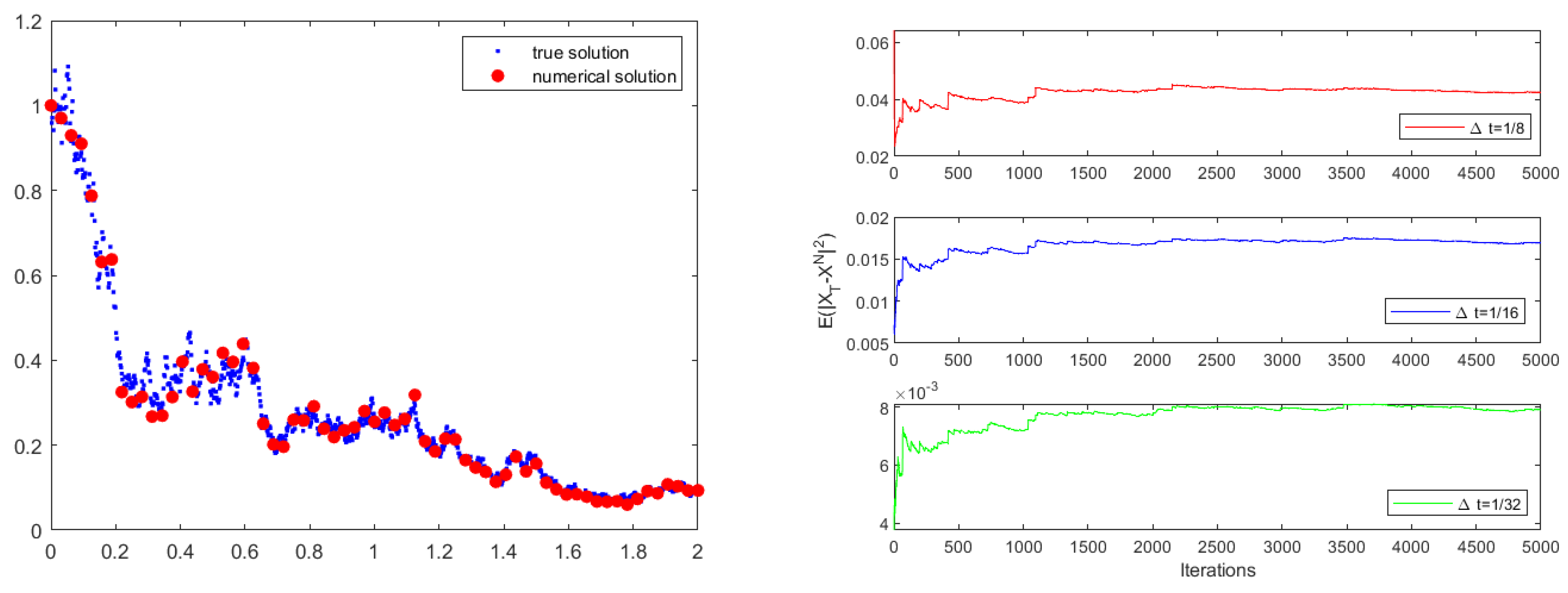
Example 1.

Consider the Mackey–Glass equation with a multiplicative noise:

$$d{X}_t=[-a{X}_t+\frac{b{X}_{t-\tau }}{1+X_{t-\tau }^2}]dt+\sigma X_{t}d{W}_t,$$

(54)

where $a>0$, and b and σ are real parameters. Next, we use Scheme 1 to solve the problem with parameters

$$a=3,b=1,\sigma =1,\tau =1,X_t=1,t\in [-1,0].$$

We approximate the “true solution” using the Euler–Maruyama method with a sufficiently small step size (here, $\mathsf{\Delta }t=2^{-10}$). In Table 1, we compare the errors, convergence rates (CR for short) and operating time of the Euler scheme, Milstein scheme and Scheme 1. The results demonstrate that Scheme 1 exhibits a superior convergence rate. In the left of Figure 1, we depict the numerical solution resulting from Scheme 1 with a step size of $\mathsf{\Delta }t=\frac{1}{32}$, alongside a sample path’s “true solution”. We obtain the mean-square convergence stability result of global errors to test stability in the right of Figure 1. The numerical results here are consistent with the results we established regarding convergence and stability.

Table 1. The results of global convergence rates and errors for three schemes in Example 1.

N	16	32	64	128	256	CR	Time(s)
Euler scheme	1.433 × ${10}^{-2}$	7.032 × ${10}^{-3}$	3.548 × ${10}^{-3}$	1.766 × ${10}^{-3}$	6.773 × ${10}^{-4}$	1.079	0.3337
Milstein scheme	1.380 × ${10}^{-2}$	6.319 × ${10}^{-3}$	3.238 × ${10}^{-3}$	1.771 × ${10}^{-3}$	5.928 × ${10}^{-4}$	1.092	0.3581
Scheme 1	1.293 × ${10}^{-2}$	3.240 × ${10}^{-3}$	1.049 × ${10}^{-3}$	3.375 × ${10}^{-4}$	2.805 × ${10}^{-5}$	2.096	0.3608

Figure 1. (Left) Path simulation; (Right) mean-square stability with different time steps $\mathsf{\Delta }t=\frac{1}{8}$, $\mathsf{\Delta }t=\frac{1}{16}$ and $\mathsf{\Delta }t=\frac{1}{32}$.

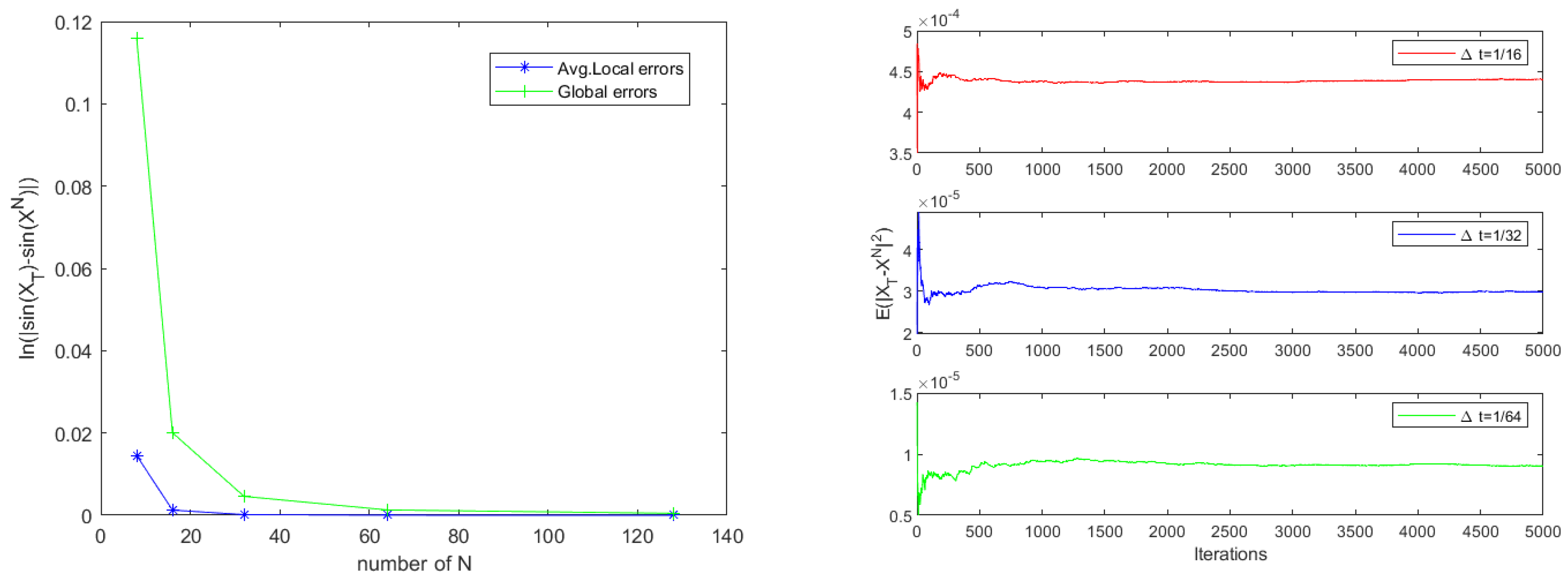
Example 2

(Square of O-U delay process). In this example, we consider nonlinear SDDEs. In order to give nonlinear SDDEs, we first study linear SDDEs:

$$\left\{\begin{array}{c}d{X}_t=\{a_1{X}_t+a_2{X}_{t-\tau }\}dt+bd{W}_t,t\in [0,T],\hfill \\ X_t=1+t,t\in [-\tau ,0],\hfill \end{array}\right.$$

(55)

with the terminal time $T=2\tau =2$.

By using the Itô formula with respect to $X_t^2$, we deduce

$$\begin{array}{cc}\hfill d\left(X_t^2\right)& =\left(2X_t(a_1{X}_t+a_2{X}_{t-\tau })+0.5\times 2b^2\right)dt+2b{X}_{t}d{W}_t\hfill \\ \hfill & =\left(b^2+2a_1{X}_t^2+2a_2{X}_t{X}_{t-\tau }\right)dt+2b{X}_{t}d{W}_t.\hfill \end{array}$$

Assuming $Y_t=X_t^2$, we have

$$\begin{array}{c}\hfill d{Y}_t=\{b^2+2a_1{Y}_t+2a_2\sqrt{Y_t}\sqrt{Y_{t-\tau }}\}dt+2b\sqrt{Y_t}d{W}_t.\end{array}$$

Therefore, we obtain the following nonlinear models for SDDEs:

$$\left\{\begin{array}{c}d{Y}_t=\{b^2+2a_1{Y}_t+2a_2\sqrt{Y_t}\sqrt{Y_{t-\tau }}\}dt+2b\sqrt{Y_t}d{W}_t,t\in [0,T],\hfill \\ Y_t=X_t^2,t\in [-\tau ,0].\hfill \end{array}\right.$$

(56)

Based on the explicit solution of Equation (55), we have the explicit solution of Equation (56) on $t\in [0,1]$:

$$Y_t=X_t^2={\left(X_0{e}^{a_{1}t}+e^{a_{1}t}{\int }_0^t{a}_{2}s{e}^{-a_{1}s}ds+b{e}^{a_{1}t}{\int }_0^t{e}^{-a_{1}s}d{W}_s\right)}^2,$$

where $X_t$ has normal distribution $\mathbb{N}\left(h\left(t\right),\sigma \left(t\right)\right)$ with the mean value $h\left(t\right)=X_0{e}^{a_{1}t}-\frac{a_2}{a_1}t{e}^{-a_{1}t}-\frac{a_2}{a_1^2}\left(e^{-a_{1}t}-1\right)$ and the variance $\sigma \left(t\right)={\displaystyle \frac{b^2}{2a_1}}\left(e^{2a_{1}t}-1\right).$ Next, we obtain the solution of Equation (56) on $t\in [1,2]$:

$$Y_t=X_t^2={\left(X_1{e}^{a_1(t-1)}+e^{a_{1}t}{\int }_1^t{a}_2{X}_{s-1}{e}^{-a_{1}s}ds+b{e}^{a_{1}t}{\int }_1^t{e}^{-a_{1}s}d{W}_s\right)}^2.$$

In this experiment, we give nonlinear SDDEs by the (O-U) process for linear SDDEs and study the property of the nonlinear SDDEs with the parameters of $a_1=-2$, $a_2=1.7$ and $b=0.01$. In Table 2, we present the error and convergence results for Example 2. For a more intuitive display, the plots of errors result with respect to N are drawn in the left of Figure 2, which implies that the experimental results are in agreement with the theoretical results. In addition, we obtain the mean-square convergence stability result of global errors with times steps $\mathsf{\Delta }t=\frac{1}{16}$, $\mathsf{\Delta }t=\frac{1}{32}$ and $\mathsf{\Delta }t=\frac{1}{64}$, which are shown in the right of Figure 2.

Table 2. The results of convergence rates and errors with constant parameters in Example 2.

N	Avg.Local Errors	CR	Global Errors	CR
8	1.576 × ${10}^{-1}$		8.102 × ${10}^{-2}$
16	2.073 × ${10}^{-2}$	2.9264	1.998 × ${10}^{-2}$	2.0196
32	2.444 × ${10}^{-3}$	3.0054	5.076 × ${10}^{-3}$	1.9991
64	2.841 × ${10}^{-4}$	3.0431	1.261 × ${10}^{-3}$	1.9985
128	3.415 × ${10}^{-5}$	3.0533	3.384 × ${10}^{-4}$	1.9790

Figure 2. (Left) The plots of global and average local errors with respect to the steps N; (Right) mean-square stability with different time steps $\mathsf{\Delta }t=\frac{1}{16}$, $\mathsf{\Delta }t=\frac{1}{32}$ and $\mathsf{\Delta }t=\frac{1}{64}$.

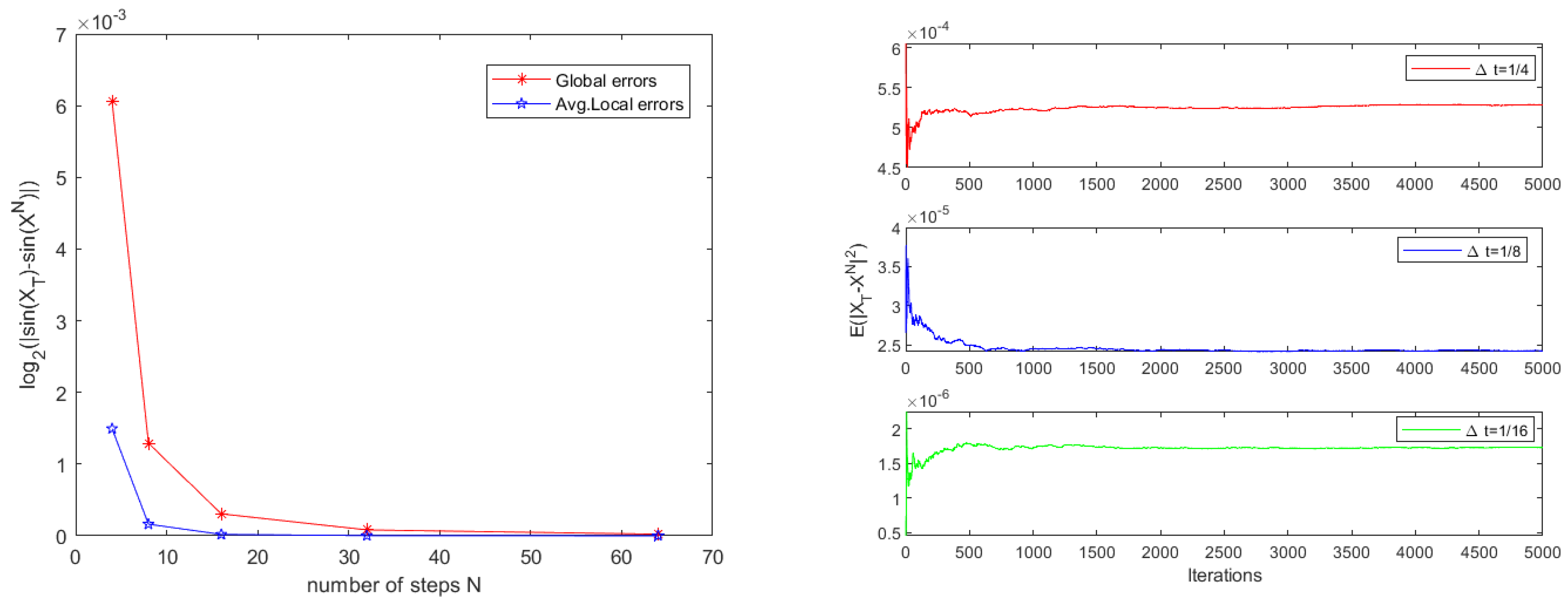
Example 3.

Consider the linear SDDE with a time-varying delay:

$$\left\{\begin{array}{c}d{X}_t=\{a_1{X}_t+a_2{X}_{t-\tau \left(t\right)}\}dt+\{b_1+b_2{X}_{t-\tau \left(t\right)}\}d{W}_t,t\in [0,T],\hfill \\ X_t=\psi \left(t\right),t\in [-\tau ,0]\hfill \end{array}\right.$$

(57)

where $\tau \left(t\right)=\frac{1+t}{2}$ and the terminal time $T=2$. Next, we give the solution of Equation (57) on $t\in [0,1]$:

$$X_t=X_0{e}^{a_{1}t}+e^{a_{1}t}{\int }_0^t{a}_2\psi (s-\tau \left(s\right))e^{-a_{1}s}ds+e^{a_{1}t}{\int }_0^t(b_1+b_2\psi (s-\tau \left(s\right)))e^{-a_{1}s}d{W}_s.$$

(58)

Next, we utilize Equation (58) to obtain a solution on $t\in [1,2]$. Therefore, Equation (57) has the solution

$$X_t=X_1{e}^{a_1(t-1)}+e^{a_{1}t}{\int }_1^t{a}_2{X}_{s-\tau \left(s\right)}{e}^{-a_{1}s}ds+e^{a_{1}t}{\int }_1^t(b_1+b_2{X}_{s-\tau \left(s\right)})e^{-a_{1}s}d{W}_s.$$

In this example, we assume $N\in \{2^2,2^3,2^4,2^5,2^6\}$. We test the convergence rate and errors of Scheme 1 by setting the delay function $\psi \left(t\right)=1+t$, $a_1=-1$, $a_2=1$, $b_1=0.01$, $b_2=0.01$; the error and convergence results are provided in Table 3. As expected, Scheme 1 can obtain global second-order and local third-order convergence rates, which are in agreement with theoretical results. We also plot the lines of average local errors (Avg.Local Errors for short) and global errors with respect to the steps N in the left of Figure 3. Furthermore, the figure intuitively displays that the theoretical results are correct. For three different time steps $\mathsf{\Delta }t=\frac{1}{4}$, $\mathsf{\Delta }t=\frac{1}{8}$ and $\mathsf{\Delta }t=\frac{1}{16}$, we obtain the mean-square convergence stability result of global errors in the right of Figure 3.

Table 3. The results of convergence rates and errors with constant parameters in Example 3.

N	Avg.Local Errors	CR	Global Errors	CR
4	1.494 × ${10}^{-3}$		6.060 × ${10}^{-3}$
8	1.621 × ${10}^{-4}$	3.2040	1.290 × ${10}^{-3}$	2.2323
16	1.918 × ${10}^{-5}$	3.1418	3.060 × ${10}^{-4}$	2.1539
32	2.737 × ${10}^{-6}$	3.0359	8.224 × ${10}^{-5}$	2.0686
64	3.020 × ${10}^{-7}$	3.0435	2.275 × ${10}^{-5}$	2.0086

Figure 3. (Left) The plots of global and average local errors with respect to the steps N; (Right) mean-square stability with different time steps $\mathsf{\Delta }t=\frac{1}{4}$, $\mathsf{\Delta }t=\frac{1}{8}$ and $\mathsf{\Delta }t=\frac{1}{16}$.

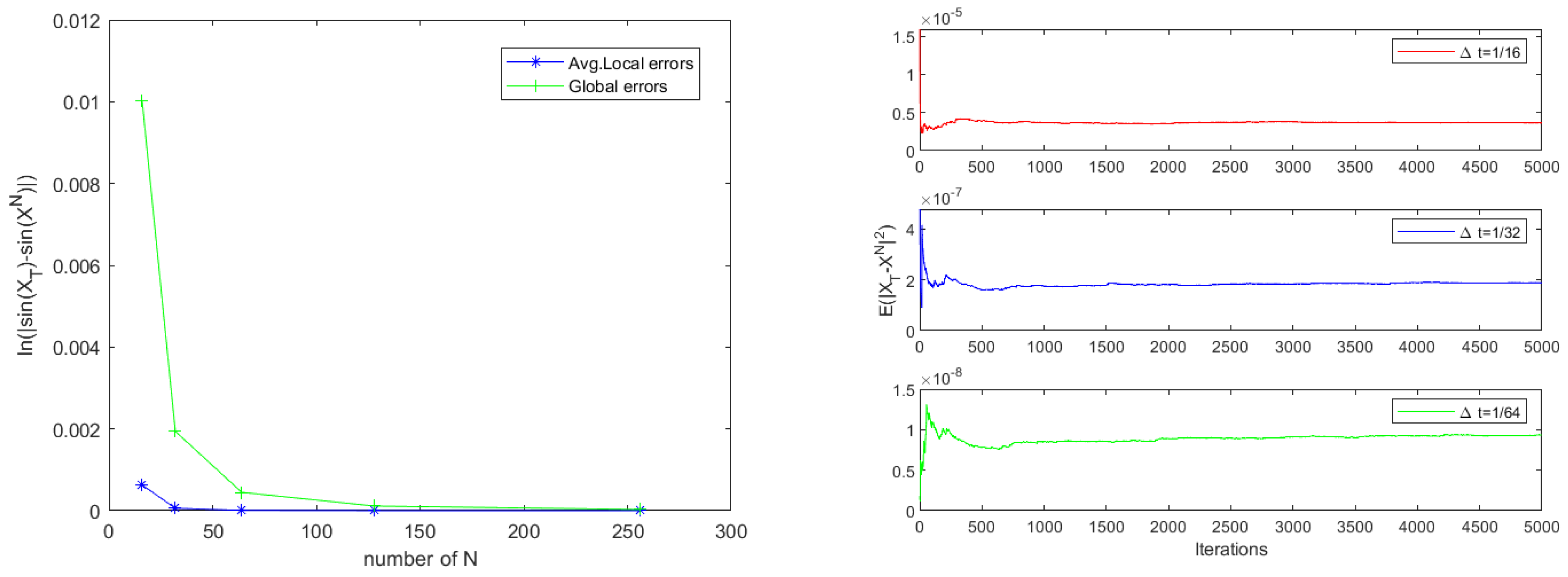
Example 4.

Consider the following two-dimensional linear SDDEs:

$$\left\{\begin{array}{c}d{X}_t=\left(\begin{array}{cc}-\lambda & 0\\ 0& -\lambda \end{array}\right)X_{t}dt+\left(\begin{array}{cc}0& \sigma \\ -\sigma & 0\end{array}\right)X_{t-\tau }d{W}_t,t\in [0,T],\hfill \\ X_t=\psi \left(t\right),t\in [-\tau ,0],\hfill \end{array}\right.$$

(59)

where $\tau =1$ and the terminal time $T=1$. Next, we use Scheme 1 to solve the problem with parameters

$$\lambda =4,\sigma =0.3,\psi \left(t\right)={(1+t,1+t)}^{\mathit{T}}.$$

In this example, it is not a simple decoupled SDDE, so it cannot be regarded as a scalar equation. With an assumption of $N\in \{16,32,64,128,256\}$, we simulate and calculate the convergence rates and errors of Scheme 1; the error and convergence results are provided in Table 4. It is gratifying that Scheme 1 can obtain global second-order and local third-order convergence rates. We also plot the lines of average local errors (Avg. Local Errors for short) and global errors with respect to the steps N in the left of Figure 4. For three different time steps $\mathsf{\Delta }t=\frac{1}{16}$, $\mathsf{\Delta }t=\frac{1}{32}$ and $\mathsf{\Delta }t=\frac{1}{64}$, we obtain the mean-square convergence stability result of global errors in the right of Figure 4. The figure intuitively displays that the theoretical results are correct.

Table 4. The results of convergence rates and errors with constant parameters in Example 4.

N	Avg.Local Errors	CR	Global Errors	CR
16	6.267 × ${10}^{-4}$		1.002 × ${10}^{-2}$
32	6.059 × ${10}^{-5}$	3.3706	1.939 × ${10}^{-3}$	2.3701
64	7.003 × ${10}^{-6}$	3.2418	4.482 × ${10}^{-4}$	2.2416
128	8.830 × ${10}^{-7}$	3.1526	1.132 × ${10}^{-4}$	2.1519
256	1.207 × ${10}^{-7}$	3.0784	3.747 × ${10}^{-5}$	2.0796

Figure 4. (Left) The plots of global and average local errors with respect to the steps N; (Right) mean-square stability with different time steps $\mathsf{\Delta }t=\frac{1}{16}$, $\mathsf{\Delta }t=\frac{1}{32}$ and $\mathsf{\Delta }t=\frac{1}{64}$.

5. Conclusions

A simplified numerical method is developed to solve SDDEs, which involves no multiple stochastic Itô-type integrals and can be easily used to solve multidimensional SDDEs. Based on the theory of Malliavin derivatives, we introduce a novel weak local convergence lemma for multiple random integrals, deriving the connecting inequality between Theorems 1 and 2. We rigorously establish in two steps that Scheme 1 exhibits a global weak second-order convergence rate. Furthermore, we present four distinct numerical examples to illustrate the efficiency, mean-square stability and convergence rates of the simplified weak high-order numerical method. Additionally, we included a dedicated discussion section to provide a detailed comparison of our approach with other existing methods in terms of computational time. According to the above experiments, we can obtain that the new scheme has the most precision of all schemes but costs more time. In future work, we will investigate higher-order numerical methods for solving SDDEs.