The Testing Procedure for the Overall Lifetime Performance Index of Rayleigh Products in Multiple Production Lines Based on the Progressive Type I Interval Censored Sample

Abstract

The lifetime performance index is a process capability index that is commonly used for the evaluation of the durability of products in life testing and reliability analysis. In the context of multiple production lines, we introduce an overall lifetime performance index and explore the relationship between this comprehensive index and individual lifetime performance indices. For products with lifespans following the Rayleigh distribution in the ith production line, we delve into the maximum likelihood estimator and asymptotic distribution to derive both the individual and overall lifetime performance indices. By establishing a predetermined target for the overall lifetime performance index, we can determine the corresponding target for each individual lifetime performance index. The testing algorithmic procedure is proposed to ascertain whether the overall lifetime performance index has reached its target value based on the maximum likelihood estimator, accompanied by figures illustrating the analysis of test power. We found that there is a monotonic relationship for the test power with various structures of parameters. Finally, a practical illustration with one numeral example is presented to demonstrate how the testing procedure is employed to evaluate the capabilities of multiple production lines.

1. Introduction

Analyzing process capability is a crucial aspect in statistical quality control applications, providing insights into whether a product aligns with the specified quality requirements. The process capability index (PCI) serves as a tool to quantify this capability by assessing the extent to which a quality characteristic meets the specified specification limit. Several widely employed process capability indices have been proposed in the literature, such as Cp, Cpk, Cpm, and Cpmk (see Juran [1], Kane [2], Hsiang and Taguchi [3], and Pearn et al. [4]). These indices were designed for bilateral specifications. For unilateral specification, Montgomery [5] proposed a process capability index $C_L=\frac{\mu -L}{\sigma }$ for the larger-the-better quality characteristic, where u, σ, and L are the process mean, standard deviation, and the lower specification limit. This index is well known as the lifetime performance index in life testing and reliability analysis. The primary emphasis of this investigation is the evaluation of the lifetime performance index C_L within the context of unilateral tolerance in multiple production lines. Unlike many process capability indices assuming a normal distribution, product lifetimes often follow distributions like gamma, exponential, Rayleigh, or other lifetime distributions. In this paper, we assume a Rayleigh distribution for the lifetime of products in each production line utilizing the lifetime performance index C_L due to the preference for longer product lifetimes. For products that are produced in a single production line, Tong et al. [6] developed a uniformly minimum variance unbiased estimator (UMVUE) for complete samples under the assumption of a one-parameter exponential distribution. In practice, many experimenters are unable to collect complete samples and can only observe incomplete ones, such as progressive censored samples. Previous studies (like those by Aggarwala [7], Balakrishnan and Aggarwala [8], Hong et al. [9], Wu et al. [10], Sanjel and Balakrishnan [11], and Lee et al. [12]) focus on drawing conclusions from data that have been censored. Additionally, for step-stress accelerated life testing data, Lee et al. [13] evaluated the lifetime performance index. Wu et al. [14] proposed a testing procedure for product lifetimes in a single production line based on progressive type I interval censored samples for Rayleigh distribution. Furthermore, Wu et al. [15] implemented an experimental design for Rayleigh products under the condition of achieving a given test power or minimizing the total experimental cost for a specific cost structure. Later on, Wu et al. [16] conducted an experimental design for the lifetime performance Index of Weibull products based on the progressive type I interval censored sample. Wu and Song [17] investigated the sampling plan for progressive type I interval censoring on the lifetime performance index of the Chen lifetime distribution. These studies are based on one production line. By extending from one production line to multiple production lines, we will define an overall lifetime performance index and explore the relationship between the overall lifetime performance index and all individual lifetime performance indices. We will develop a testing procedure to see if the overall lifetime performance index reaches the target value through the use of the maximum likelihood estimator and its asymptotic normal distribution for a given level of significance. Our aim for this research is to propose an overall lifetime performance index and design a testing procedure for this index to determine if the whole production process is capable with multiple production lines. This is a study that extends from analyzing one single production line to multiple production lines. The motivation for this study stems from the fact that many manufacturing processes consist of multiple production lines.

The progressive type I interval censoring is delineated as follows: Initially, a set of products of size n undergoes a life test starting at time 0. The inspection times are predetermined and denoted as (t₁, …, t_m), where t_m is the scheduled termination time of the experiment. At each inspection time t_i, the number of observed failures X_i is recorded during the interval (t_i−1,t_i), and then R_i products are removed from the remaining products. This process continues until the experiment concludes at time t_m, where the number of failures X_m is observed during the interval (t_m−1,t_m), and all of the remaining items are removed and lead to the termination of the life test.

Our primary objective is to formulate a hypothesis testing procedure for the overall lifetime performance index by using the maximum likelihood estimator as the test statistic based on the progressive type I interval censored sample collected from multiple production lines, assuming a Rayleigh distribution. The shape of the Rayleigh distribution is skewed to the right, and it is an asymmetric probability distribution. Therefore, this research applies the asymmetric probability distribution model to the field of lifetime performance assessment in quality control.

The subsequent sections of this paper are structured as follows: In Section 2, the overall lifetime performance index is defined for products produced in multiple production lines. The relationship between the overall lifetime performance index and all individual lifetime performance indices is also explored. In Section 3.1, we delve into the study of the maximum likelihood estimator (MLE) for the overall lifetime performance index and all individual lifetime performance indices and explore their asymptotic normal distributional properties. This is accomplished based on the progressive type I interval censored samples from multiple production lines, assuming a Rayleigh distribution. In Section 3.2, we present a testing algorithmic procedure designed for the overall lifetime performance index under a given level of significance, which equivalently tests all individual lifetime performance indices. With the aim of illustrating our proposed testing procedure, one numerical example is provided to illustrate the application of the proposed testing procedure. Finally, Section 4 encapsulates the paper with concluding remarks.

2. The Overall Lifetime Performance Index and the Conforming Rate

We consider products produced in d production lines. Suppose that the lifetime U_i of products in the ith production line follows a Rayleigh distribution with the probability density function (pdf), cumulative distribution function (cdf), and hazard function, as follows:

$$f\left(u\right)=\frac{u}{{\lambda }_i^2}{e}^{-\frac{u^2}{2{\lambda }_i^2}},u\ge 0,{\lambda }_i>0,$$

(1)

$$F\left(u\right)=1-e^{-\frac{u^2}{2{\lambda }_i^2}}, u\ge 0,{\lambda }_i>0$$

(2)

and

$$h\left(u\right)=\frac{f\left(u\right)}{1-F\left(u\right)}=\frac{u}{{{\lambda }_i}^2},$$

(3)

where ${\lambda }_i$ is the scale parameter, i = 1, …, d. The larger-the-better type process capability index proposed in Montgomery [5] is defined as

$$C_L=\frac{\mu -L}{\sigma },$$

(4)

where $\mu$ represents the process mean, $\sigma$ represents the process standard deviation, and $L$ denotes the specified lower specification limit. This index is also called the lifetime performance index (LPI) for products. Consider the transformation of $Y_i=U_i^2$; then, the new lifetime $Y_i$ has a one-parameter exponential distribution with pdf, cdf, and hazard functions as

$$f\left(y\right)=\frac{1}{{2\lambda }_i^2}{e}^{-\frac{\mathrm{y}}{2{{\lambda }_i}^2}},y\ge 0,{\lambda }_i>0,$$

(5)

$$F\left(y\right)=1-e^{-\frac{\mathrm{y}}{2{{\lambda }_i}^2}}, y\ge 0,{\lambda }_i>0$$

(6)

and

$$h\left(y\right)=\frac{f\left(y\right)}{1-F\left(y\right)}=\frac{1}{{2{\lambda }_i}^2}$$

(7)

The mean and standard deviation of the new lifetime are ${\mu }_i=E\left(Y_i\right)=2{\lambda }_i^2, { \sigma }_i=\sqrt{Var\left(Y_i\right)}=2{\lambda }_i^2,i=1,\dots , d$. The lifetime performance index $C_{L_i}$ for the ith production line is reduced to

$$C_{L_i}=\frac{\mu -L_i}{\sigma }=\frac{2{\lambda }_i^2-L_i}{2{\lambda }_i^2}=1-\frac{L_i}{2{\lambda }_i^2},i=1,\dots , d.$$

(8)

It can be observed that the lifetime performance index $C_{L_i}$ can precisely evaluate the long-term performance of products, since the smaller the hazard function, the larger the lifetime performance index $C_{L_i}$.

The ith production line’s conformity rate is defined as the probability that the product’s lifetime will exceed the lower specification limit L_i, and it is obtained as

$$P_{r_i}=P\left(Y_i\ge L_i\right)={\int }_{L_i}^{\infty }\frac{1}{2{\lambda }_i^2}{e}^{-\frac{y}{2{\lambda }_i^2}}dy=e^{-\frac{L_i}{2{\lambda }_i^2}}=e^{C_{L_i}-1},-\infty <C_{L_i}<1.$$

(9)

Apparently, the conforming rate for the ith production line increases when the lifetime performance index $C_{L_i}$ increases. For example, if the user wishes $P_{r_i}$ to be over 0.860708, then they can determine that the value of $C_{L_i}$ must be 0.95 from Equation (9).

We assume that the lifetimes of products in d production lines are independent. The overall conforming rate $P_r$ for d production lines is computed as

$$\begin{gathered} P_r=P\left(Y_i\ge L_i, i=1,\cdots ,d\right) \\ =\exp \left\{-\sum _{i=1}^d\frac{L_i}{2{\lambda }_i^2}\right\}=\exp \left\{\sum _{i=1}^d{C}_{L_i}-d\right\},-\infty <C_{L_i}<1. \end{gathered}$$

We define the overall lifetime performance index C_T as $P_r=\mathrm{e}\mathrm{x}\mathrm{p}\left\{\sum _{i=1}^d{C}_{L_i}-d\right\}=\mathrm{e}\mathrm{x}\mathrm{p}\left\{C_T-1\right\},-\infty <C_T<1$ so that the overall conforming rate $P_r$ is an increasing function of the overall lifetime performance index C_T. To solve this equation, we can find the relationship between the overall lifetime performance index and all individual lifetime performance indices as

$$C_T=\sum _{i=1}^d{C}_{L_i}-\left(d-1\right),-\infty <C_T<1.$$

(10)

Under the reasonable consideration of $C_{L_1}=\dots =C_{L_d}=C_L$, the relationship between the individual lifetime performance index $C_L$ and the overall lifetime performance index C_T becomes

$$C_L=\frac{C_T+d-1}{d},-\infty <C_T<1.$$

(11)

For example, if the engineer wished the target value of the overall lifetime performance index to be $C_T=$c₀, the individual lifetime performance index $C_L$ for each production line can be determined by $C_L=\frac{C_0+d-1}{d}$. For example, if the experimenter desires the target value of the overall lifetime performance index to be $C_T=$ c₀ = 0.95, then the desired target value for each production line can be determined from Equation (11) as $C_L$ = 0.975, 0.98333, 0.9875, 0.99, 0.99166, 0.99285, 0.99375, 0.99444, or 0.995 for d = 2, 3, …, 10.

3. The Testing Procedure for the Overall Lifetime Performance Index

In this section, the maximum likelihood estimator and the asymmetric distribution of the overall lifetime performance index and each individual lifetime performance index are investigated in Section 3.1. To test whether the overall lifetime performance index reaches the desired target level, the testing procedure and the power analysis for various structures of parameters are given in Section 3.2. In Section 3.3, we give one numerical example to demonstrate how to apply our proposed testing procedure.

3.1. Maximum Likelihood Estimator of the Lifetime Performance Index

For the ith production line, the progressive type I interval censored sample $X_{i1},\dots ,X_{im}$ is collected at the observation times $t_1,\dots ,t_m$ under the progressive censoring scheme of $R_1,\dots ,R_m$. The likelihood function for the censored sample $X_{i1},\dots ,X_{im}$ is

$$\begin{gathered} L\left({\lambda }_i\right)\propto \prod _{j=1}^m{\left(F\left(t_j\right)-F\left(t_{j-1}\right)\right)}^{x_{ij}}{\left(1-F\left(t_j\right)\right)}^{R_{ij}} \\ \propto \prod _{j=1}^m{\left(1-e^{-\frac{t_j^2-t_{j-1}^2}{2{\lambda }_i^2}}\right)}^{x_{ij}}{e}^{-\frac{t_{j-1}^2{x}_{ij}+t_j^2{R}_{ij}}{2{\lambda }_i^2}}. \end{gathered}$$

(12)

The log-likelihood function is

$$\ln L\left({\lambda }_i\right)\propto {\sum }_{j=1}^m\left\{x_{ij}\ln \left[1-\exp \left(-A_{ij}\right)\right]-B_{ij} \right\},$$

(13)

where $A_{ij}=\frac{t_j^2-t_{j-1}^2}{2{\lambda }_i^2},B_{ij}=\frac{t_{j-1}^2{x}_{ij}+t_j^2{R}_{ij}}{2{\lambda }_i^2},i=1,\dots ,d,j=1,\dots ,m.$ When taking the derivative for the parameter ${\lambda }_i$ from Equation (12), the log-likelihood equation becomes

$$\frac{d}{d{\lambda }_i}lnL\left({\lambda }_i\right)=-\frac{1}{{\lambda }_i^3}\sum _{j=1}^m{x}_{ij}\left(\frac{t_j^2-t_{j-1}^2}{\exp \left(\frac{t_j^2-t_{j-1}^2}{2{\lambda }_i^2}\right)-1}-\left(t_{j-1}^2{x}_{ij}+t_j^2{R}_{ij}\right)\right)=0.$$

(14)

By numerically solving the log-likelihood Equation in (14), we can obtain the maximum likelihood estimator (MLE) of ${\lambda }_i$ denoted by ${\widehat{\lambda }}_i$.

In order to find the asymptotic variance of the estimator ${\widehat{\lambda }}_i$, the Fisher’s information number $I\left({\lambda }_i\right)=-E\left[\frac{d^2\mathit{ln}L\left({\lambda }_i\right)}{d{\lambda }_i^2}\right]$ needs to be computed. By taking the second derivative to the likelihood function in (12), we have

$$\begin{gathered} \frac{d^2\ln L\left({\lambda }_i\right)}{d{\lambda }_i^2}=\sum _{j=1}^m\left[\frac{-X_{ij}}{{\left[\exp \left(\frac{{t_j}^2-{t_{j-1}}^2}{2{\lambda }_i^2}\right)-1\right]}^2}\exp \left(\frac{{t_j}^2-{t_{j-1}}^2}{2{\lambda }_i^2}\right){\left(\frac{{t_j}^2-{t_{j-1}}^2}{{\lambda }_i^3}\right)}^2\right] \\ +\frac{x_{ij}}{\exp \left(\frac{{t_j}^2-{t_{j-1}}^2}{2{\lambda }_i^2}\right)-1}\frac{3\left({t_j}^2-{t_{j-1}}^2\right)}{{\lambda }_i^4}-\frac{3\left({t_{j-1}}^2{x}_{ij}+{{t_j}^{2}R}_{ij}\right)}{{\lambda }_i^4} \end{gathered}$$

(15)

Note that

$$\left.X_{ij}\right|X_{i,j-1},\dots ,X_{i1}~\mathrm{Binomial}\left(n-{\displaystyle \sum _{l=1}^{j-1}{X}_{il}},q_{ij}\right),$$

(16)

where $q_{ij}=\frac{\left.F{\left(t\right.}_j)-F{\left(t\right.}_{j-1}\right)}{\left.1-F{\left(t\right.}_{j-1}\right)}=1-\mathrm{e}\mathrm{x}\mathrm{p}\left(-\frac{{t_j}^2-{t_{j-1}}^2}{2{\lambda }_i^2}\right),j=1,\cdots ,m.$

Hence, we have

$$E\left(\left.X_{ij}\right|X_{i,j-1},\cdots ,X_{i1},R_{i,j-1},\cdots ,R_{i1}\right)==n{q}_{ij}{\displaystyle \prod _{l=1}^{j-1}\left(1-p_l\right)\left(1-q_{il}\right)},j=1,\cdots ,m\hspace{0.33em}.$$

(17)

Hence, the Fisher’s information number is

$$\begin{gathered} I\left({\lambda }_i\right)=\frac{n}{{\lambda }_i^2}\sum _{j=1}^m\left\{\frac{1-q_{ij}}{q_{ij}}\left[4{ln}^2\left(1-q_{ij}\right)+6q_{ij}\mathit{ln}\left(1-q_{ij}\right)\right] \\ +\frac{3\left(t_{j-1}^2{q}_{ij}+t_j^2{p}_{ij}\left(1-q_{ij}\right)\right)}{{\lambda }_i^2}\right\}\prod _{l=1}^{j-1}\left(1-p_{il}\right)\left(1-q_{il}\right), \end{gathered}$$

(18)

According to the distributional property of the maximum likelihood estimator, we have ${\widehat{\lambda }}_i\underset{n\to \mathrm{\infty }}{\stackrel{d}{\to }}\mathrm{N}\left({\lambda }_i,I^{-1}\left({\lambda }_i\right)\right)$.

For likelihood-based inferences, Guillermo et al. [18] estimated the parameters for the asymmetric beta-skew alpha-power distribution by considering the maximum likelihood method, and the Fisher information matrix was derived. For other censoring schemes, like the combined generalized progressive hybrid censoring scheme, Seong and Lee [19] found the conditional maximum likelihood estimator for the scale parameter of exponential distribution. For the confidence intervals for binomial distribution in Equation (16), Jäntschi [20] proposed three alternative confidence interval calculation methods and algorithms to improve the nominal coverage probabilities compared to the Wald asymptotic interval method. Félix et al. [21] improved the performance of several confidence intervals, including the Wald, Wilson score, and arcsine confidence intervals, by using the parametric family ${\widehat{p}}_c=\frac{X+c}{n+2c}$ with c ≥ 0 to estimate the parameter p, where X is the number of successes out of n trials. Rather than using the confidence intervals approach, their analysis was conducted based on the hypothesis test approach. They identified the values of c that result in the optimal testing procedure.

Based on the invariance property of the maximum likelihood estimator, the maximum likelihood estimator of $C_{L_i}$ is obtained as

$${\widehat{C}}_{L_i}=1-\frac{L_i}{2{\widehat{\lambda }}_i^2}.$$

(19)

Using the Delta method, we can show that

$${\widehat{C}}_{L_i}\underset{n\to \mathrm{\infty }}{\stackrel{d}{\to }}\mathrm{N}\left(C_{L_i},V\left({\widehat{C}}_{L_i}\right)\right)$$

(20)

where ${\widehat{V}}_i\left({\widehat{C}}_{L_i}\right)=\frac{L_i^2\widehat{V}\left({\widehat{\lambda }}_i\right)}{{\widehat{\lambda }}_i^6}=\frac{L_i^2{I}^{-1}\left({\widehat{\lambda }}_i\right)}{{\widehat{\lambda }}_i^6}$.

Based on the invariance property of the maximum likelihood estimator, the maximum likelihood estimator of C_T is

$${\widehat{C}}_T={\sum }_{i=1}^d{\widehat{C}}_{L_i}-\left(d-1\right)$$

(21)

Its asymptotic distribution is ${\widehat{C}}_T\underset{n\to \mathrm{\infty }}{\stackrel{d}{\to }}\mathrm{N}\left(C_T,\sum _{i=1}^d\widehat{V}\left({\widehat{C}}_{L_i}\right)\right),$ where the variance of ${\widehat{C}}_T$ is ${\sum }_{i=1}^{d}V\left({\widehat{C}}_{Li}\right)$ and its estimate is ${\sum }_{i=1}^d\widehat{V}\left({\widehat{C}}_{Li}\right)={\sum }_{i=1}^d\frac{L_i^2{I}^{-1}\left({\widehat{\lambda }}_i\right)}{{\widehat{\lambda }}_i^6}$.

3.2. The Testing Procedure for the Overall Lifetime Performance Index and Power Analysis

For the assessment of whether the overall lifetime performance index exceeds the desired target value c₀, we develop a statistical testing procedure in this section. The null and alternative hypotheses are $H_0:C_T\le c_0$ (d production lines are not capable) vs. $H_a:C_T>c_0$ (d production lines are capable). Under the condition of $C_{L1}=\cdots =C_{Ld}{=C}_L$, if the overall lifetime performance index is $C_T={\displaystyle \sum _{i=1}^k{C}_{Li}}-(k-1)>c_0$, we can obtain the condition of $C_{Li}>c_0^{*},\hspace{0.33em}i=1,\dots ,d$, where the target value for each individual lifetime performance index is $c_0^{*}=\frac{c_0+k-1}{k}$. The above statistical hypothesis for testing the overall lifetime performance index is equivalently set up as follows:

$H_0:C_{Li}\le c_0^{*}$ for some i (d production lines are not capable) vs. $H_a:C_{Li}>c_0^{*},i=1,\dots ,d$ (d production lines are capable). This is called an intersection–union test (IUT). In order to find the rejection region by controlling the overall error rate, we use the following theorem:

Theorem 1. 

To test $H_0:C_{Li}\le c_0^{*}$ for some i vs. $H_a:C_{Li}>c_0^{*},i=1,\dots ,d$ with level α, the rejection region for this test is $R={\displaystyle \underset{i=1}{\overset{k}{\cap }}{R}_i}$, where $R_i=\left\{{\widehat{C}}_{Li}\left|{\widehat{C}}_{Li}>C_{Li}^0\right.\right\}\hspace{0.33em}$, the test statistic is ${\widehat{C}}_{L_i}=1-\frac{L_i}{2{\widehat{\lambda }}_i^2}$, the critical value is $C_{L_i}^0=1-\frac{L_i}{2{\left({\lambda }_{i0}+Z_{{\alpha }^{\prime }}\sqrt{I^{-1}\left({\lambda }_{i0}\right)}\right)}^2}$, i = 1, …, d, and ${\lambda }_{i0}=\sqrt{\frac{L_i}{2\left(1-c_0^{*}\right)}}$. The proof of Theorem 1 is given in Appendix A.

The algorithm for conducting a testing procedure for C_T is shown below (Algorithm 1).

Algorithm 1. Testing procedure for the overall lifetime performance index

Step 1: For the pre-assigned target level $c_0$ for the overall lifetime performance index, the required target level for each individual lifetime performance index is determined as $c_0^{*}=\frac{c_0+k-1}{k}$ for each production line. Then the testing hypothesis $H_0:C_{Li}\le c_0^{*}$ for some i vs. $H_a:C_{Li}>c_0^{*},i=1,\dots ,d$ are constructed. Step 2: Under the known lower specification $L_i,$ observe the progressive type I interval censored sample $X_{i1},\dots ,X_{im}$ at the observation times $t_1,\dots ,t_m$ with censoring schemes of $R,\dots ,R_m$ from the Rayleigh distribution. Step 3: Compute the value of the test statistic ${\widehat{C}}_{L_i}=1-\frac{L_i}{2{\widehat{\lambda }}_i^2},$ where ${\widehat{\lambda }}_i$ is obtained by solving Equation (14). Step 4: For significance level of $\alpha ,$ we can calculate the critical value $C_{L_i}^0=1-\frac{L_i}{2{\left({\lambda }_{i0}+Z_{{\alpha }^{\prime }}\sqrt{I^{-1}\left({\lambda }_{i0}\right)}\right)}^2}$$\mathrm{where} {\lambda }_{i0}=\sqrt{\frac{L_i}{2\left(1-c_0^{*}\right)}}$, ${\mathsf{\alpha }}^{\prime }={\alpha }^{\raisebox{1ex}{$1$}\!\left/ \!\raisebox{-1ex}{$d$}\right.}$$\mathrm{and} I^{-1}\left({\lambda }_{i0}\right)$ is defined in Equation (18). Step 5: If ${\widehat{C}}_{Li}>C_L^0$$\mathrm{for} \mathrm{all} i=1,\dots ,d$, we can concluded that the overall lifetime performance index of the products adhered the required level.

Furthermore, the test power function $h\left(c_1\right)$ of the testing procedure at the point of $C_T=d{C}_L-(d-1)=c_1>c_0$ or $C_L=\frac{c_1+d-1}{d}=c_1^{*}$ can be obtained as follows:

$$h\left(c_1\right)=P\left({\widehat{C}}_{L_i}>C_{L_i}^0,i=1,\cdots ,d |{ c}_1^{*}=1-\frac{L_i}{2{\lambda }_{i1}^2},i=1,\cdots ,d\right)$$

Let ${\lambda }_{i1}=\sqrt{\frac{L_i}{2\left(1-c_1^{\mathrm{*}}\right)}}$ and ${\lambda }_{i0}=\sqrt{\frac{L_i}{2\left(1-c_0^{\mathrm{*}}\right)}}$. Then, the power function becomes

$$\begin{array}{l}h\left(c_1\right)=P(1-\frac{L_i}{2{\widehat{\lambda }}_i^2}>1-\frac{L_i}{2{\left({\lambda }_{i0}+Z_{{\alpha }^{\prime }}\sqrt{I^{-1}\left({\lambda }_{i0}\right)}\right)}^2},i=1,\cdots ,d)\\ =P({\widehat{\lambda }}_i>{\lambda }_{i0}+Z_{{\alpha }^{\prime }}\sqrt{I^{-1}\left({\lambda }_{i0}\right)},i=1,\cdots ,d)\\ ={\displaystyle \prod _{i=1}^d}P({\widehat{\lambda }}_i>{\lambda }_{i0}+Z_{{\alpha }^{\prime }}\sqrt{I^{-1}\left({\lambda }_{i0}\right)})\\ ={\displaystyle \prod _{i=1}^d}P(\frac{{\widehat{\lambda }}_i-{\lambda }_{i1}}{\sqrt{I^{-1}\left({\lambda }_{i1}\right)}}>\frac{{\lambda }_{i0}-{\lambda }_{i1}+Z_{{\alpha }^{\prime }}\sqrt{I^{-1}\left({\lambda }_{i0}\right)}}{\sqrt{I^{-1}\left({\lambda }_{i1}\right)}})\\ ={\prod }_{i=1}^d\left[1-\mathsf{\Phi }\left(\frac{{\lambda }_{i0}-{\lambda }_{i1}+Z_{{\alpha }^{\prime }}\sqrt{I^{-1}\left({\lambda }_{i0}\right)}}{\sqrt{I^{-1}\left({\lambda }_{i1}\right)}}\right)\right]\end{array}$$

(22)

where $\mathsf{\Phi }\left(\cdot \right)$ is the cdf for the standard normal distribution.

Under $L_1=\dots =L_k=L$, the power function is reduced to

$$h\left(c_1\right)={\left[1-\mathsf{\Phi }\left(\frac{{\lambda }_0{-\lambda }_1+Z_{{\alpha }^{\prime }}\sqrt{I^{-1}\left({\lambda }_0\right)}}{\sqrt{I^{-1}\left({\lambda }_1\right)}}\right)\right]}^d,$$

(23)

where ${\lambda }_1=\sqrt{\frac{L}{2\left(1-c_1^{\mathrm{*}}\right)}}$ and ${\lambda }_0=\sqrt{\frac{L}{2\left(1-c_0^{\mathrm{*}}\right)}}$.

The powers h(c₁) for testing $H_0:C_L\le 0.85$ are computed by Equation (23), and we use R software for programming. The powers are tabulated in Table A1, Table A2, Table A3, Table A4, Table A5, Table A6, Table A7, Table A8 and Table A9 for d = 2, 3, and 4 with α = 0.01, 0.02, and 0.05, respectively, for c₁ = 0.85, 0.885, 0.9, 0.915, 0.93, and 0.96; m = 5, 6, and 7; n = 70, 90, and 110; and p = 0.050, 0.075 and 0.1 under L = 0.05 and T = 0.5. The power values are showcased in Figure 1, Figure 2, Figure 3, Figure 4 and Figure 5 using the values from Table A1, Table A2, Table A3, Table A4, Table A5, Table A6, Table A7, Table A8 and Table A9 to exemplify several standard cases. We obtain the following findings: (1) In Figure 1, it can be seen that the power is an increasing function of n under d = 3, α = 0.02, m = 5, and p = 0.01 (other combinations of d, m, p, and α also show the same pattern). (2) In Figure 2, it can be seen that the power increases when m increases under d = 3, n = 110, p = 0.01, and α = 0.02 (other combinations of d, n, p, and α also show the same pattern). (3) In Figure 3, the power is a decreasing function of p under d = 3, n = 110, m = 5, and α = 0.02 (other combinations of d, n, m, and α also have the same pattern). (4) In Figure 4, the power is an increasing function of α under d = 3, n = 110, m = 5, and p = 0.01 (other combinations of d, n, m, and p also have the same pattern). (5) In Figure 5, the power is a decreasing function of d under n = 110, m = 5, p = 0.01, and α = 0.02 (other combinations of n, m, p, and α also have the same pattern). The difference of power converges when c₁ increases. (6) In Figure 1, Figure 2, Figure 3, Figure 4 and Figure 5 the power is an Increasing function of the value of c₁ under various combinations of d, n, m, p, and $\alpha .$

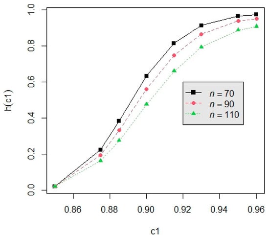
Figure 1. The power curves under d = 3, α = 0.02, m = 5, p = 0.01, and n = 70, 90, and 110.

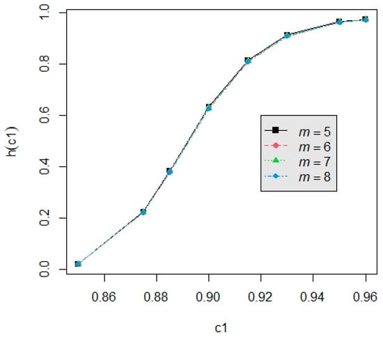
Figure 2. The power curves under d = 3, α = 0.02, n = 110, p = 0.01, and m = 5, 6, 7, and 8.

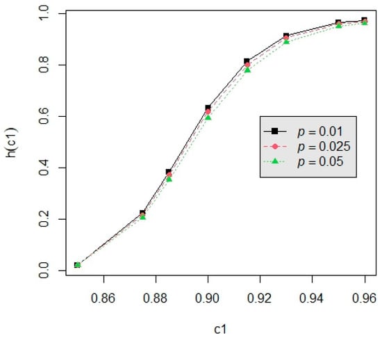
Figure 3. The power curves under d = 3, α = 0.02, n = 110, m = 5, and p = 0.01, 0.025, and 0.05.

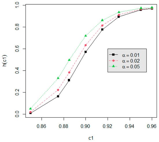
Figure 4. The power curves under d = 3, n = 110, m = 5, p = 0.01, and α = 0.01, 0.02, and 0.05.

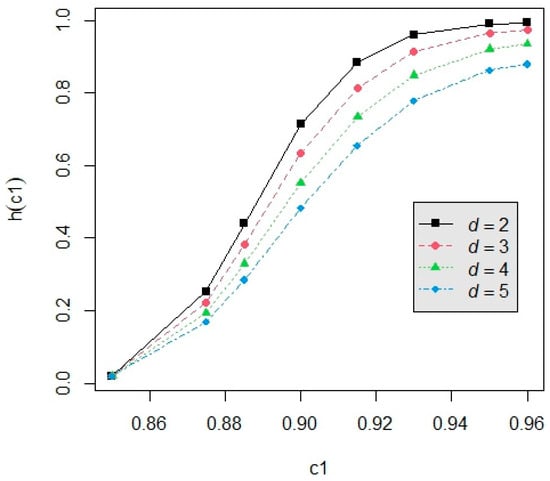
Figure 5. The power curves under n = 30, m = 5, p = 0.01, α = 0.02, and d = 1, 2, 3, 4, and 5.

3.3. Example

We regard the sample data in Caroni [22], consisting of the failure times of ball bearings of n = 20, as the lifetimes in the first production line. The data are listed as follows: 0.1788, 0.2892, 0.4152, 0.4212, 0.4560, 0.4880, 0.5184, 0.5196, 0.5412, 0.5556, 0.6780, 0.6844, 0.6864, 0.6888, 0.9312, 0.9864, 1.0512, 1.0584, 1.2804, 1.7340. We use the Gini statistic proposed in Gail and Gastwirth [23] to test the goodness of fit of the Rayleigh distribution, and the value of the test statistic does not fall into the rejection region, so these data fit the Rayleigh distribution well. We regard the sample data in Aarset [24], consisting of the failure times of n = 50 devices, as the lifetimes in the second production line. The data are listed as follows: 0.01, 0.02, 0.1, 0.1, 0.1, 0.1, 0.1, 0.2, 0.3, 0.6, 0.7, 1.1, 1.2, 1.8, 1.8, 1.8, 1.8, 1.8, 2.1, 3.2, 3.6, 4.0, 4.5, 4.5, 4.7, 5.0, 5.5, 6.0, 6.3, 6.3, 6.7, 6.7, 6.7, 6.7, 7.2, 7.5, 7.9, 8.2, 8.2, 8.3, 8.4, 8.4, 8.4, 8.5, 8.5, 8.5, 8.5, 8.5, 8.6, 8.6. The Gini test in Gail and Gastwirth [19] is used to test the goodness of fit of the Rayleigh distribution, and the p-value is 0.538 > 0.05, so the test results support the Rayleigh distribution.

Suppose we want to test $H_0:C_T\le 0.85\hspace{0.33em}vs\hspace{0.33em}{H}_1:C_T>0.85$. Furthermore, we create the progressive type I interval censored sample for the failure times of products from two production lines. Let the termination time be T = 2.0 and let the number of inspections be m = 5; the equal length of inspection interval is t = 0.1 (thousand cycles), and the pre-specified removal percentages of the remaining survival units are given by the following: (p₁, p₂, p₃, p₄, p₅) = (0.05, 0.05, 0.05, 0.05, 1.0).

Using the algorithm of the testing procedure for the overall lifetime performance index, the testing procedure is implemented as follows:

Step 1: Given the known lower specification L₁ = L₂ = L = 0.05 and at the observation times ($t_1,\dots ,t_5$) = (0.4, 0.8, 1.2, 1.6, 2.0), we collect the progressive type I interval censored sample, (X₁₁, X₁₂, X₁₃, X₁₄, X₁₅) = (2, 9, 5, 1, 0) and (X₂₁, X₂₂, X₂₃, X₂₄, X₂₅) = (9, 2, 1, 0, 2), for each production line with censoring schemes of (R₁₁, R₁₂, R₁₃, R₁₄, R₁₅) = (1, 1, 1, 0, 0) and (R₂₁, R₂₂, R₂₃, R₂₄, R₂₅) = (1, 1, 1, 1, 2).

Step 2: Under the required level, $c_0$ = 0.85, we can determine the required level to be 0.925 for each production line: $c_0^{*}=\frac{c_0+k-1}{k}=\frac{0.85+2-1}{2}$ = 0.925. Equivalently, we can test the null hypothesis $H_0:C_{Li}\le 0.925$ for some i vs. $H_a:C_{Li}>0.925,i=1,2$.

Step 3: For two production lines, we can obtain the maximum likelihood estimators for two production lines as ${\widehat{\lambda }}_1=$ 0.6055 and ${\widehat{\lambda }}_2$ = 0.8789. Then, we can compute the values of the testing statistic as ${\widehat{C}}_{L_1}=1-\frac{L_1}{2{\widehat{\lambda }}_1^2}=1-\frac{0.05}{2\times {\left(0.6055\right)}^2}=0.9318 \mathrm{a}\mathrm{n}\mathrm{d} {\widehat{C}}_{L_2}=1-\frac{L_2}{2{\widehat{\lambda }}_2^2}=1-\frac{0.05}{2\times {\left(0.8789\right)}^2}=0.9676$.

Step 4: For the level of significance of α = 0.1, we have ${\alpha }^{\prime }={0.1}^{\frac{1}{2}}=0.3162$ and ${\mathsf{\lambda }}_{i0}={\mathsf{\lambda }}_{20}=\sqrt{\frac{L_i}{2\left(1-{\mathrm{c}}_0^{\mathrm{*}}\right)}}=\sqrt{\frac{0.05}{2\times \left(1-0.925\right)}}=0.5774$. The critical values are obtained as $C_{L_1}^0=C_{L_2}^0=1-\frac{L_i}{2{\left({\lambda }_{i0}+Z_{{\alpha }^{\prime }}\sqrt{I^{-1}\left({\lambda }_{i0}\right)}\right)}^2}=1-\frac{0.05}{2{\left(0.5774+\left(-0.4782\right)\times 0.0048\right)}^2}=0.9156$ for two production lines.

Step 5: Since ${\widehat{C}}_{L_1}>C_{L_1}^0$ and ${\widehat{C}}_{L_2}>C_{L_2}^0,$ we can conclude that the overall lifetime performance index has attained the required target level since all individual lifetime performance indices have reached their corresponding desired target values.

4. Conclusions

In numerous manufacturing sectors, the examination of lifetime performance indices for products is a crucial area of focus, particularly when a product’s lifespan adheres to a Rayleigh distribution. For products that are produced in multiple production lines, with each one following a Rayleigh distribution for its lifetime, we introduce an overall lifetime performance index for these multiple production lines. Our investigation delves into the correlation between the overall lifetime performance index and individual lifetime performance indices. We examine the maximum likelihood estimator and asymptotic distribution for both the individual and overall lifetime performance indices in the context of progressive type I interval censored samples. To evaluate whether the overall lifetime performance index attains the desired target level, we devise a hypothesis testing procedure. This method entails testing each individual lifetime performance index using the maximum likelihood estimator as the test statistic. We explore the influences of different configurations of the sample size n, the number of inspection intervals m, the removal probability p, the level of significance α, and the number of production lines d on the test power using graphical representations and table values, with a specific focus on the number of production lines. All findings are also outlined. We found that the test power is an increasing function of n, m, and α when the other parameters are fixed. We also found that the test power is a decreasing function of p and d when the other parameters are fixed. To illustrate the application of our proposed testing algorithm for the overall lifetime performance index with two production lines, we provide one numerical example in the conclusion.

References

- Juran, J.M. Juran’s Quality Control Handbook, 3rd ed.; McGraw-Hill: New York, NY, USA, 1974. [Google Scholar]
- Kane, V.E. Process capability indices. J. Qual. Technol. 1986, 18, 41–52. [Google Scholar] [CrossRef]
- Hsiang, T.C.; Taguchi, G. A tutorial on quality control and assurance—The Taguchi mthods. In Proceedings of the Joint Meetings of the American Statistical Association—ASA Annual Meeting, Las Vegas, NV, USA, 5–8 August 1985; p. 188. [Google Scholar]
- Pearn, W.L.; Kotz, S.; Johnson, N.L. Distributional and inferential properties of process capability indices. J. Qual. Technol. 1992, 24, 216–231. [Google Scholar] [CrossRef]
- Montgomery, D.C. Introduction to Statistical Quality Control; John Wiley and Sons Inc.: New York, NY, USA, 1985. [Google Scholar]
- Tong, L.I.; Chen, K.S.; Chen, H.T. Statistical testing for assessing the performance of lifetime index of electronic components with exponential distribution. Int. J. Qual. Reliab. Manag. 2002, 19, 812–824. [Google Scholar] [CrossRef]
- Aggarwala, R. Progressive interval censoring: Some mathematical results with applications to inference. Commun. Stat.-Theory Methods 2001, 30, 1921–1935. [Google Scholar] [CrossRef]
- Balakrishnan, N.; Aggarwala, R. Progressive Censoring: Theory, Methods and Applications; Birkhäuser: Boston, MA, USA, 2000. [Google Scholar]
- Hong, C.W.; Lee, W.C.; Wu, J.W. Computational Procedure of Performance Assessment of Lifetime Index of Products for the Weibull Distribution with the Progressive First-Failure-Censored Sampling Plan. J. Appl. Math. 2012, 2012, 717184. [Google Scholar] [CrossRef]
- Wu, J.W.; Lee, W.C.; Lin, L.S.; Hong, M.L. Bayesian test of lifetime performance index for exponential products based on the progressively type II right censored sample. J. Quant. Manag. 2011, 8, 57–77. [Google Scholar]
- Sanjel, D.; Balakrishnan, N. A Laguerre polynomial approximation for a goodness-of-fit test for exponential distribution based on progressively censored data. J. Stat. Comput. Simul. 2008, 78, 503–513. [Google Scholar] [CrossRef]
- Lee, W.C.; Wu, J.W.; Hong, C.W. Assessing the lifetime performance index of products with the exponential distribution under progressively type II right censored samples. J. Comput. Appl. Math. 2009, 231, 648–656. [Google Scholar] [CrossRef]
- Lee, H.M.; Wu, J.W.; Lei, C.L. Assessing the Lifetime Performance Index of Exponential Products With Step-Stress Accelerated Life-Testing Data. IEEE Trans. Reliab. 2013, 62, 296–304. [Google Scholar] [CrossRef]
- Wu, S.F.; Lin, Y.T.; Chang, W.J.; Chang, C.W.; Lin, C. A computational algorithm for the evaluation on the lifetime performance index of products with Rayleigh distribution under progressive type I interval censoring. J. Comput. Appl. Math. 2018, 328, 508–519. [Google Scholar] [CrossRef]
- Wu, S.F.; Liu, T.H.; Lai, Y.H.; Chang, W.T. A study on the experimental design for the lifetime performance index of Rayleigh lifetime distribution under progressive type I interval censoring. Mathematics 2022, 10, 517. [Google Scholar] [CrossRef]
- Wu, S.F.; Wu, Y.C.; Wu, C.H.; Chang, W.T. Experimental design for the lifetime performance Index of Weibull products based on the progressive type I interval censored sample. Symmetry 2021, 13, 1691. [Google Scholar] [CrossRef]
- Wu, S.F.; Song, M.Z. The experimental design for the progressive type I interval censoring on the lifetime performance index of Chen lifetime distribution. Mathematics 2023, 11, 1554. [Google Scholar] [CrossRef]
- Guillermo, M.F.; Roger, T.F.; Marvin, J.N. Likelihood-Based Inference for the Asymmetric Beta-Skew Alpha-Power Distribution. Symmetry 2020, 12, 613. [Google Scholar]
- Seong, Y.; Lee, K. Exact Likelihood Inference for Parameter of Exponential Distribution under Combined Generalized Progressive Hybrid Censoring Scheme. Symmetry 2022, 14, 1764. [Google Scholar] [CrossRef]
- Jäntschi, L. Binomial Distributed Data Confidence Interval Calculation: Formulas, Algorithms and Examples. Symmetry 2022, 14, 1104. [Google Scholar] [CrossRef]
- Félix, A.A.; Hortensia, R.C.; Marcos, M.C. A comparison of some confidence intervals for a binomial proportion based on a shrinkage estimator. Open Math. 2023, 21, 20220588. [Google Scholar]
- Caroni, C. Modeling the reliability of ball bearings. J. Stat. Educ. 2002, 10, 1–8. [Google Scholar] [CrossRef][Green Version]
- Gail, M.H.; Gastwirth, J.L. A sacle-free goodness-of-fit Test for the Exponential Distribution Based on the Gini Statistic. J. R. Stat. Soc. Ser. B (Methodol.) 1978, 40, 350–357. [Google Scholar]
- Aarset, M.V. How to identify a bathtub hazard rate. IEEE Trans. Reliab. 1987, 36, 106–108. [Google Scholar] [CrossRef]
Disclaimer/Publisher’s Note: The statements, opinions and data contained in all publications are solely those of the individual author(s) and contributor(s) and not of MDPI and/or the editor(s). MDPI and/or the editor(s) disclaim responsibility for any injury to people or property resulting from any ideas, methods, instructions or products referred to in the content. |
© 2024 by the authors. Licensee MDPI, Basel, Switzerland. This article is an open access article distributed under the terms and conditions of the Creative Commons Attribution (CC BY) license (https://creativecommons.org/licenses/by/4.0/).