A Symmetry of Boundary Functions Method for Solving the Backward Time-Fractional Diffusion Problems

Abstract

In the paper, we develop three new methods for estimating unknown initial temperature in a backward time-fractional diffusion problem, which is transformed to a space-dependent inverse source problem for a new variable in the first method. Then, the initial temperature can be recovered by solving a second-order boundary value problem. The boundary functions and a unique zero element constitute a group symmetry. We derive energetic boundary functions in the symmetry group as the bases to retrieve the source term as an unknown function of space and time. In the second method, the solution bases are energetic boundary functions, and then by collocating the governing equation we obtain the expansion coefficients for retrieving the entire solution and initial temperature. For the first two methods, boundary fluxes are over-specified to retrieve the initial condition. In the third method, we give two boundary conditions and a final time temperature to construct the bases in another symmetry group; the governing equation is collocated to a linear system to obtain the whole solution (initial temperature involved). These three methods are assessed and compared by numerical experiments.

1. Introduction

The time-fractional diffusion equation has many practical applications in anomalous sub-diffusion and random walk models [1,2,3], as well as some complicated dynamical systems in fields such as semi-conductors, porous media, life science, and economy finance, etc. [4,5,6]. We consider

$$\begin{array}{c}{D}_t^{\alpha }T(x,t)=T_{xx}(x,t)+\rho (x,t),(x,t)\in (0,a)\times (0,t_f],\hfill \end{array}$$

(1)

$$\begin{array}{cc}\hspace{1em}\hspace{1em}\hspace{1em}\hspace{1em}\hspace{1em} \hfill & T(0,t)=T_0\left(t\right),T(a,t)=T_a\left(t\right),T_x(0,t)=Q_0\left(t\right),T_x(a,t)=Q_a\left(t\right),\hfill \end{array}$$

(2)

and give the over-specified data:

$$\rho (0,t)={\rho }_0\left(t\right),\rho (a,t)={\rho }_a\left(t\right),{\rho }_x(0,t)={\rho }_{x0}\left(t\right),{\rho }_x(a,t)={\rho }_{xa}\left(t\right),$$

(3)

for recovering an unknown source $\rho (x,t)$, which depends on space and time.

The Caputo’s time-fractional derivative $D_t^{\alpha }T(x,t)$ is [7,8,9]:

$$D_t^{\alpha }T(x,t)=\frac{1}{\Gamma (1-\alpha )}{\int }_0^t\frac{T_s(x,s)}{{(t-s)}^{\alpha }}ds,0<\alpha <1.$$

(4)

Many works on the above inverse source problem suppose that $\rho (x,t)$ can be split into a product $G\left(x\right)F\left(t\right)$, and $G\left(x\right)$ or $F\left(t\right)$ is known in advance. In order to identify $G\left(x\right)$ or $F\left(t\right)$, the final time data are required, and a regularization is developed to recover the unknown source function [10,11,12,13,14,15,16,17]. In this paper, we merely use the boundary measurements to recover the source function of space and time.

The time-fractional derivative and its extension to variant order have many physical applications [18]. Besides the time-fractional diffusion equation, lots of scholars have developed many schemes to cope with the time fractional Burgers’ equation, like the operator splitting approach and artificial boundary method [19], the nonuniform Alikhanov formula of the Caputo time fractional derivative and Fourier spectral approximation in space [20], the L1 scheme and the local discontinuous Galerkin method [21], the Lucas polynomials coupled with finite difference method [22], the fourth-order compact difference scheme [23], the L1 implicit difference scheme based on non-uniform meshes [24], a second-order energy stable and nonuniform time-stepping scheme [25], a collocation approach with trigonometric tension B-splines [26], the cubic B-spline functions and $\theta$-weighted scheme [27], the local projection stabilization virtual element method [28], a compact difference scheme [29], the Caputo–Katugampola fractional derivative by extending the Laplace transform [30], and the tailored finite point method based on exponential basis [31]. For the time-fractional Schrödinger equations, lots of researchers have proposed many algorithms, like the conformable natural transform and the homotopy perturbation method [32], the conformable fractional derivatives modified Khater technique and the Adomian decomposition method [33], the Laplace Adomian decomposition method and the modified generalized Mittag–Leffler function method [34], a Caputo residual power series scheme [35], and the extended Kudryashov method [36].

The solution to the backward time-fractional diffusion problem is to recover the initial temperature. By

$$T(x,t)=u(x,t)-g\left(x\right),$$

where the initial temperature $g\left(x\right)$ is an unknown function, we can transform Equation (1) to an inverse source problem for $u(x,t)$:

$$D_t^{\alpha }u(x,t)=u_{xx}(x,t)-g^{\prime \prime }\left(x\right)+\rho (x,t).$$

By applying the inverse source technique we can recover $g^{\prime \prime }\left(x\right)$, and it becomes a second-order boundary value problem for $g\left(x\right)$. We are going to solve the backward time-fractional diffusion problem by two novel methods, which merely require the boundary data.

Liu and Yamamoto [37] described this sort-backward problem for the porous media-related diffusion process with continuous time random walks. Practically, it is of great importance because the initial density of substance is not often known, but the density at a positive moment can be measured to provide a final time condition. In general, for a better solution of the backward problem, some regularization techniques were used [38,39,40,41,42].

For seeking an accurate solution of the fractional partial differential equation (PDE), a key issue is the development of a very precise numerical method to compute the fractional derivative term at discretized points. However, for the fractional PDE, only limited approaches of the Laplace transformation, the Fourier transformation and the iteration method are available [43,44]. Currently, there are high-order finite difference method [45,46,47], the Grünwald–Letnikov method [48], Diethelm’s method [49,50], and the combination of Diethelm’s method and Hadamard’s finite-part integral [51]. In the paper, we will develop particular bases in terms of space and time explicitly, such that by equipping with the Gaussian quadrature, we can generate a linear equations system with very accurate coefficients matrix and right-hand vector to solve the time-fractional partial differential equation with high accuracy.

The rest of the paper’s contents proceed as follows. In Section 2, we develop a symmetry of boundary functions method to solve the inverse source problem under over-specified boundary data; a certain group symmetry is set up for the construction of bases, and a set of energetic boundary functions is created. Section 3 derives the linear equations system to recover the source term, which is a function of space and time. Numerical experiments to solve the inverse source problems are given in Section 4. We solve the backward time-fractional diffusion problems in Section 5 with three novel methods being developed. In Section 6, numerical experiments to solve the backward time-fractional diffusion problems are given. Finally, we conclude the main achievements in Section 7.

2. A Method of Symmetry of Boundary Functions

To be used throughout the paper, we derive the following formula:

$$\Gamma (1-\alpha )={\int }_0^1(e^{-t}{t}^{-\alpha }+e^{-1/t}{t}^{\alpha -2})dt.$$

(5)

In the paper, we will apply the three-point Gaussian quadrature to compute the integral terms in Equations (4) and (5).

Let $\nu =1-\alpha$. Starting from the definition of Gamma function:

$$\Gamma \left(\nu \right)={\int }_0^{\infty }{e}^{-t}{t}^{\nu -1}dt,$$

(6)

we divide it into two sub-integrals:

$$\Gamma \left(\nu \right)={\int }_1^{\infty }{e}^{-t}{t}^{\nu -1}dt+{\int }_0^1{e}^{-t}{t}^{\nu -1}dt.$$

(7)

Take $\tau =1/t$ in the first integral,

$${\int }_1^{\infty }{e}^{-t}{t}^{\nu -1}dt={\int }_1^0{e}^{-1/\tau }{\tau }^{1-\nu }\frac{-d\tau }{{\tau }^2}={\int }_0^1{e}^{-1/\tau }{\tau }^{-1-\nu }d\tau .$$

(8)

Then, we can compute $\Gamma \left(\nu \right)$ by

$$\Gamma \left(\nu \right)={\int }_0^1(e^{-t}{t}^{\nu -1}+e^{-1/t}{t}^{-\nu -1})dt,$$

(9)

which is a definite integral, and the three-point Gaussian quadrature is applicable. Taking $\nu =1-\alpha$ in Equation (9), we can derive Equation (5).

Equation (1) is multiplied by $T(x,t)$:

$$T(x,t)D_t^{\alpha }T(x,t)=T_{xx}(x,t)T(x,t)+\rho (x,t)T(x,t).$$

By integration it follows that

$${\int }_0^{a}T(x,t)D_t^{\alpha }T(x,t)dx+{\int }_0^a{T}_x^2(x,t)dx-{\int }_0^a\rho (x,t)T(x,t)dx=F\left(t\right),$$

(10)

where

$$F\left(t\right):=Q_a\left(t\right)T_a\left(t\right)-Q_0\left(t\right)T_0\left(t\right)$$

(11)

is obtained from Equation (2).

To set up a group symmetry, let

$$u(x,t)=T(x,t)-H^T(x,t)$$

(12)

be a new variable, where a homogeneous function for $T(x,t)$:

$$\begin{array}{c}{H}^T(x,t)=\frac{x^3}{a^3}[2T_0\left(t\right)-2T_a\left(t\right)+a{Q}_0\left(t\right)+a{Q}_a\left(t\right)]\hfill \\ -\frac{x^2}{a^2}[3T_0\left(t\right)-3T_a\left(t\right)+2a{Q}_0\left(t\right)+a{Q}_a\left(t\right)]+x{Q}_0\left(t\right)+T_0\left(t\right)\hfill \end{array}$$

(13)

matches all boundary conditions in Equation (2):

$$H^T(0,t)=T_0\left(t\right),H^T(a,t)=T_a\left(t\right),H_x^T(0,t)=Q_0\left(t\right),H_x^T(a,t)=Q_a\left(t\right);$$

(14)

hence, by Equations (12) and (14),

$$u(0,t)=0,u(a,t)=0,u_x(0,t)=0,u_x(a,t)=0.$$

(15)

It follows from Equations (10) and (12) that

$$\begin{array}{c}{\int }_0^a[u(x,t)+H^T(x,t)][D_t^{\alpha }u(x,t)+D_t^{\alpha }{H}^T(x,t)]dx+{\int }_0^a{[u_x(x,t)+H_x^T(x,t)]}^{2}dx\hfill \\ -{\int }_0^a[u(x,t)+H^T(x,t)]\rho (x,t)dx=F\left(t\right).\hfill \end{array}$$

(16)

First, we introduce a family of homogenization functions:

$$B^j\left(x\right)=(x^4-2a{x}^3+a^2{x}^2)x^{j-1},j\ge 1,$$

(17)

which satisfy

$$B^j\left(0\right)=0,B^j\left(a\right)=0,B_x^j\left(0\right)=0,B_x^j\left(a\right)=0.$$

(18)

Recall that a group consists of a non-empty set G and a binary operation + on G, satisfying the following conditions [52]:

(a)

For any two $g_1,g_2\in G$, $g_1+g_2\in G$ (closure property).

(b)

$(g_1+g_2)+g_3=g_1+(g_2+g_3)$ for any $g_1,g_2,g_3\in G$ (associativity).

(c)

There is a unique zero element $0\in G$, such that $0+g=g+0=g\in G$ (zero element).

(d)

For every $g\in G$ there is a unique element $-g\in G$, such that $-g+g=g+(-g)=0\in G$ (inverse element).

An addition group denoted by $\mathcal{G}$ consists of a zero element and the set of all boundary functions:

$$\left\{B^j\left(x\right)\right\},j\ge 1,$$

(19)

subjecting to Equation (18).

Theorem 1.

In Equation (1), $\rho (x,t)$ can be approximately recovered by solving the following functional equation:

$$\begin{array}{c}{\int }_0^a[H^T(x,t)+E^j\left(x\right)]\rho (x,t)dx\hfill \\ ={\int }_0^a[H^T(x,t)+E^j\left(x\right)]D_t^{\alpha }{H}^T(x,t)dx+{\int }_0^a{[E_x^j\left(x\right)+H_x^T(x,t)]}^{2}dx-F\left(t\right),\hfill \end{array}$$

(20)

where

$$E^j\left(x\right)={\gamma }_j{B}^j\left(x\right)+B^{j+1}\left(x\right),j\ge 1,$$

(21)

are elements in the symmetry group $\mathcal{G}$. In Equation (21),

$${\gamma }_j=\frac{-e_1-\sqrt{e_1^2-4e_0{e}_2}}{2e_2},$$

(22)

where

$$\begin{array}{cc}\hfill & e_2={\int }_0^a{B}_x^j{\left(x\right)}^{2}dx,\hfill \\ \hfill & e_1={\int }_0^a\{2[B_x^{j+1}\left(x\right)+H_x^T(x,t)]B_x^j\left(x\right)+[D_t^{\alpha }{H}^T(x,t)-\rho (x,t)]B^j\left(x\right)\}dx,\hfill \\ \hfill & e_0={\int }_0^a\{{[B_x^{j+1}\left(x\right)+H_x^T(x,t)]}^2+[D_t^{\alpha }{H}^T(x,t)-\rho (x,t)][B^{j+1}\left(x\right)+H^T(x,t)]\}dx-F\left(t\right).\hfill \end{array}$$

(23)

Proof. 

It permits $E^j\left(x\right)\in \mathcal{G}$ in Equation (21) with the closure property of group:

$$E^j\left(0\right)=0,E^j\left(a\right)=0,E_x^j\left(0\right)=0,E_x^j\left(a\right)=0.$$

(24)

The group reflects a certain symmetry of the set of all boundary functions. Next, we determine ${\gamma }_j$ for each $E^j\left(x\right)$.

The symmetry $\mathcal{G}$ involves $u(x,t)$ as a particular element, since $u(x,t)$ satisfies the boundary conditions in Equation (15). Because of $E^j\left(x\right)\in \mathcal{G}$ and $u(x,t)\in \mathcal{G}$, in the energetic identity (16), $u(x,t)$ is approximately replaced by $E^j\left(x\right)$; hence, the energetic functional Equation (20) was derived, where $D_t^{\alpha }{E}^j\left(x\right)=0$ was taken into account.

By Equations (20) and (21), and

$$E_x^j\left(x\right)={\gamma }_j{B}_x^j\left(x\right)+B_x^{j+1}\left(x\right),$$

(25)

we can derive

$$e_2{\gamma }_j^2+e_1{\gamma }_j+e_0=0,$$

(26)

where $e_2$, $e_1$, and $e_0$ were given in Equation (23). The solution of Equation (26) for ${\gamma }_j$ is given by Equation (22). Moreover, $E^j\left(x\right)\in \mathcal{G}$, $E^j\left(x\right)$ also satisfying Equation (20) are called the energetic boundary functions. □

3. The Recovery of Source Term

Let

$$\rho (x,t)=H^{\rho }(x,t)+\sum _{i=1}^m{c}_i{E}^i\left(x\right),$$

(27)

where

$$\begin{array}{c}{H}^{\rho }(x,t)=\frac{x^3}{a^3}[2{\rho }_0\left(t\right)-2{\rho }_a\left(t\right)+a{\rho }_{x0}\left(t\right)+a{\rho }_{xa}\left(t\right)]\hfill \\ -\frac{x^2}{a^2}[3{\rho }_0\left(t\right)-3{\rho }_a\left(t\right)+2a{\rho }_{x0}\left(t\right)+a{\rho }_{xa}\left(t\right)]+x{\rho }_{x0}\left(t\right)+{\rho }_0\left(t\right)\hfill \end{array}$$

(28)

satisfies all conditions in Equation (3). Since $E^i\left(x\right)$ satisfies Equation (24), the advantage for Equation (27) is that $\rho (x,t)$ automatically satisfies all over-specified conditions in Equation (3).

Inserting Equation (27) for $\rho (x,t)$ into Equation (20) and taking $j=1,\dots ,m$, yields

$$\begin{array}{c}\sum _{i=1}^m{c}_i{\int }_0^a{E}^i\left(x\right)[H^T(x,t)+E^j\left(x\right)]dx\hfill \\ ={\int }_0^a[H^T(x,t)+E^j\left(x\right)][D_t^{\alpha }{H}^T(x,t)-H^{\rho }(x,t)]dx\hfill \\ +{\int }_0^a{[E_x^j\left(x\right)+H_x^T(x,t)]}^{2}dx-F\left(t\right),j=1,\dots ,m,\hfill \end{array}$$

(29)

which are m linear equations to determine m coefficients $c_i$.

The method of using the symmetry of boundary functions is depicted as follows. (i) Give $t\in (0,t_f]$, m, $\epsilon$, ${\gamma }_j=0$, $E^j\left(x\right)=B^{j+1}\left(x\right)$, and ${\mathbf{c}}^0={(c_1^0,\dots ,c_m^0)}^T$. (ii) Do $k=0,1,\dots$,

$$\rho (x,t)=H^{\rho }(x,t)+\sum _{j=1}^m{c}_j^k{E}^j\left(x\right),$$

and calculate $e_2$, $e_1$ and $e_0$ by Equation (23). (iii) Calculate ${\gamma }_j$ by Equation (22). (iv) Insert $E^j\left(x\right)={\gamma }_j{B}^j\left(x\right)+B^{j+1}\left(x\right)$ and $E_x^j\left(x\right)={\gamma }_j{B}_x^j\left(x\right)+B_x^{j+1}\left(x\right)$ into

$$\begin{array}{c}\sum _{i=1}^m{c}_i{\int }_0^a{E}^i\left(x\right)[H^T(x,t)+E^j\left(x\right)]dx\hfill \\ ={\int }_0^a[H^T(x,t)+E^j\left(x\right)][D_t^{\alpha }{H}^T(x,t)-H^{\rho }(x,t)]dx+{\int }_0^a{[E_x^j\left(x\right)+H_x^T(x,t)]}^{2}dx-F\left(t\right),\hfill \end{array}$$

and solve it to obtain ${\mathbf{c}}^{k+1}$, until

$$\parallel {\mathbf{c}}^{k+1}-{\mathbf{c}}^k\parallel \le \epsilon ;$$

otherwise, go to (ii).

4. Testing Inverse Source Problems

Let $R\left(i\right)\in [-1,1]$ be random errors in the noisy boundary measured data:

$$\begin{array}{c}\widehat{T}(0,t_i)=T_0\left(t_i\right)[1+sR\left(i\right)],\widehat{T}(a,t_i)=T_a\left(t\right)[1+sR\left(i\right)],{\widehat{T}}_x(0,t_i)=Q_0\left(t_i\right)[1+sR\left(i\right)],\hfill \\ {\widehat{T}}_x(a,t)=Q_a\left(t_i\right)[1+sR\left(i\right)],\hfill \\ \widehat{\rho }(0,t_i)={\rho }_0\left(t_i\right)[1+sR\left(i\right)],\widehat{\rho }(a,t_i)={\rho }_a\left(t_i\right)[1+sR\left(i\right)],{\widehat{\rho }}_x(0,t_i)={\rho }_{x0}\left(t_i\right)[1+sR\left(i\right)],\hfill \\ {\widehat{\rho }}_x(a,t_i)={\rho }_{xa}\left(t_i\right)[1+sR\left(i\right)].\hfill \end{array}$$

(30)

Example 1.

Consider

$$T(x,t)=e^{-t}sinx,\rho (x,t)=[D_t^{\alpha }\left(e^{-t}\right)+e^{-t}]sinx.$$

(31)

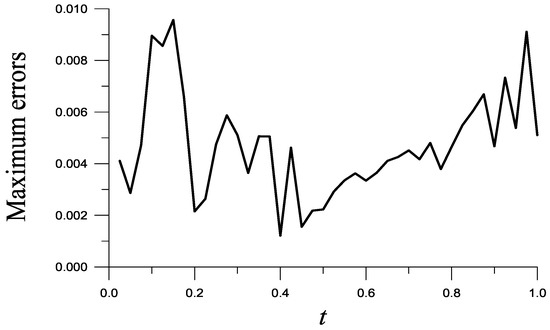
Take $\alpha =0.2$ and $s=2\%$. Good result is obtained as shown in Figure 1 to show the maximal absolute errors vs. t for the recovery of $\rho (x,t)$. The maximum error (ME) over the plane $[0,1]\times (0,1]$ is $9.57\times {10}^{-3}$, and the root-mean-square-error (RMSE) is $1.04\times {10}^{-5}$. Without the aid of the data of ${\rho }_x(0,t)={\rho }_{x0}\left(t\right)$ and ${\rho }_x(a,t)={\rho }_{xa}\left(t\right)$, ME raises to $7.18\times {10}^{-2}$.

Figure 1. For Example 1, showing maximum errors with respect to time.

Example 2.

We recover a more complex $\rho (x,t)$ from

$$T(x,t)=t+x^2+x^3+exp\left(x{t}^2\right).$$

(32)

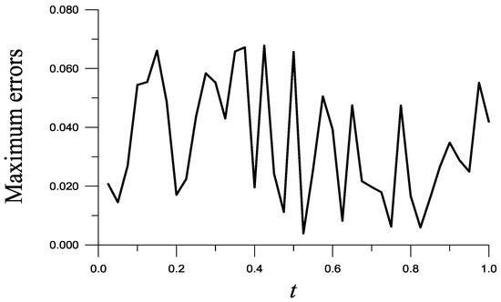
Take $\alpha =0.5$ and $s=1\%$. ME is $6.78\times {10}^{-2}$ as shown in Figure 2, and RMSE = $6.8\times {10}^{-4}$ is obtained. Notice that $max\left(\right|\rho (x,t)\left|\right)$ = 7.83, which reveals that the recovered function $\rho (x,t)$ with ME = $6.78\times {10}^{-2}$ is very accurate. When ${\rho }_x(0,t)={\rho }_{x0}\left(t\right)$ and ${\rho }_x(a,t)={\rho }_{xa}\left(t\right)$ are not given, ME raises to $0.284$.

Figure 2. For Example 2, showing maximum errors with respect to time.

Example 3.

We further consider

$$T(x,t)=e^{x+t}cos\left(xt\right).$$

(33)

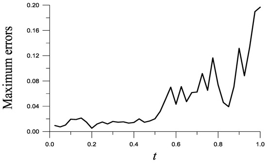
With $\alpha =0.8$, $s=2\%$, $m=2$ and $\epsilon ={10}^{-1}$, we obtain ME = $0.197$ in Figure 3, and RMSE = $2.05\times {10}^{-3}$. The value of $max\left(\right|\rho (x,t)\left|\right)$ = 11.8 is noticed, which reveals that the recovered function $\rho (x,t)$ with ME = $0.197$ is very accurate. Without taking ${\rho }_x(0,t)={\rho }_{x0}\left(t\right)$ and ${\rho }_x(a,t)={\rho }_{xa}\left(t\right)$ into account, ME raises to $0.291$.

Figure 3. For Example 3, showing maximum errors with respect to time.

Example 4.

We consider [17]:

$$T(x,t)=t^{2}sin\left(\pi x\right),\rho (x,t)=\left[\frac{\Gamma \left(3\right)}{\Gamma (3-\alpha )}{t}^{2-\alpha }+{\pi }^2{t}^2\right]sin\left(\pi x\right).$$

(34)

Table 1 lists ME, RMSE and the maximum value of $\rho (x,t)$. We fix $s=2\%$, $\alpha =0.7$, $a=0.5$, and vary $t_f$. Good results are obtained.

Table 1. For Example 4, solved by the proposed method, listing some results.

${\mathit{t}}_{\mathit{f}}$	0.4	0.6	0.7	0.8	0.9	1
ME	$1.36\times {10}^{-2}$	$2.87\times {10}^{-2}$	$3.82\times {10}^{-2}$	$4.91\times {10}^{-2}$	$6.13\times {10}^{-2}$	$7.47\times {10}^{-2}$
RMSE	$1.04\times {10}^{-2}$	$1.75\times {10}^{-2}$	$2.26\times {10}^{-2}$	$2.86\times {10}^{-2}$	$3.54\times {10}^{-2}$	$4.32\times {10}^{-2}$
Max$\left|\rho \right|$	2.13	4.49	5.98	7.67	9.57	11.68

5. Backward Time-Fractional Diffusion Problems

From now on we discuss the backward time-fractional diffusion problem of

$$\begin{array}{c}{D}_t^{\alpha }v(x,t)=v_{xx}(x,t)+S(x,t),(x,t)\in (0,a)\times (0,t_f],\hfill \end{array}$$

(35)

$$\begin{array}{cc}\hspace{1em}\hspace{1em}\hspace{1em}\hspace{1em} \hfill & v(0,t)=v_0\left(t\right),v(a,t)=v_a\left(t\right),v_x(0,t)=q_0\left(t\right),v_x(a,t)=q_a\left(t\right),\hfill \end{array}$$

(36)

where $S(x,t)$ is given, and $v_0\left(t\right)$, $v_a\left(t\right)$, $q_0\left(t\right)$, and $q_a\left(t\right)$ are given functions of time. The unknown initial condition

$$v(x,0)=g\left(x\right)$$

(37)

is to be recovered.

5.1. First Method

Let

$$T(x,t)=v(x,t)-g\left(x\right)$$

(38)

be a new variable, where $g\left(x\right)$ satisfies the compatibility conditions:

$$g\left(0\right)=v_0\left(0\right),g\left(a\right)=v_a\left(0\right),g^{\prime }\left(0\right)=q_0\left(0\right),g^{\prime }\left(a\right)=q_a\left(0\right).$$

(39)

Equation (1) is derived again by inserting Equation (38) for $v(x,t)$ into Equation (35), of which

$$\rho (x,t)=S(x,t)+g^{\prime \prime }\left(x\right).$$

(40)

Now, $g^{\prime \prime }\left(x\right)$ is an unknown function of x; however, $S(x,t)$ to be a given function is known.

We can apply the inverse source technique developed in Section 3 to recover $g^{\prime \prime }\left(x\right)$ in $\rho (x,t)$. Equations (2) and (3) are changed to

$$\begin{array}{c}T(0,t)=T_0\left(t\right)=v_0\left(t\right)-v_0\left(0\right),T(a,t)=T_a\left(t\right)=v_a\left(t\right)-v_a\left(0\right),\hfill \\ T_x(0,t)=Q_0\left(t\right)=q_0\left(t\right)-q_0\left(0\right),T_x(a,t)=Q_a\left(t\right)=q_a\left(t\right)-q_a\left(0\right),\hfill \\ \rho (0,t)={\rho }_0\left(t\right)=S(0,t)+g^{\prime \prime }\left(0\right),\rho (a,t)={\rho }_a\left(t\right)=S(a,t)+g^{\prime \prime }\left(a\right),\hfill \end{array}$$

(41)

$$\begin{array}{cc}\hspace{1em}\hfill & {\rho }_x(0,t)={\rho }_{x0}\left(t\right)=S_x(0,t)+g^{\prime \prime \prime }\left(0\right),{\rho }_x(a,t)={\rho }_{xa}\left(t\right)=S_x(a,t)+g^{\prime \prime \prime }\left(a\right).\hfill \end{array}$$

(42)

When $\rho (x,t)$ is obtained from Equation (27),

$$g^{\prime \prime }\left(x\right)=H^{\rho }(x,t)+\sum _{i=1}^m{c}_i{E}^i\left(x\right)-S(x,t)$$

(43)

can be obtained from Equation (40).

Equation (43) under the given boundary conditions $g\left(0\right)=v_0\left(0\right)$ and $g\left(a\right)=v_a\left(0\right)$ is a second-order boundary value problem. We take

$$g\left(x\right)=g\left(0\right)+\frac{x}{a}[g\left(a\right)-g\left(0\right)]+\sum _{j=1}^m{a}_{j}sin\frac{j\pi x}{a}.$$

(44)

Differentiating twice,

$$g^{\prime \prime }\left(x\right)=\sum _{j=1}^m{a}_j\frac{j^2{\pi }^2}{a^2}sin\frac{j\pi x}{a}.$$

(45)

Collocating $N_1$ points $x_k=ka/(N_1+1),k=1,\dots ,N_1$ inside the interval, we obtain a linear system:

$$\sum _{j=1}^m{a}_j\frac{j^2{\pi }^2}{a^2}sin\frac{j\pi x_k}{a}=S(x_k,t_f)-H^{\rho }(x_k,t_f)-\sum _{i=1}^m{c}_i{E}^i\left(x_k\right),k=1,\dots ,N_1.$$

(46)

Solving this system for $a_j$ and inserting them into Equation (44), we can recover the initial temperature $g\left(x\right)=v(x,0)$.

5.2. Second Method

We take

$$v(x,t)=H^v(x,t)+\sum _{j=1}^m{a}_j{E}^j\left(x\right),$$

(47)

where $E^j\left(x\right)$ can be definitely constructed from Equations (21)–(23), without needing of iteration, because $\rho (x,t)$ is replaced by $S(x,t)$, and $H^T(x,t)$ is replaced by

$$\begin{array}{c}{H}^v(x,t)=\frac{x^3}{a^3}[2v_0\left(t\right)-2v_a\left(t\right)+a{q}_0\left(t\right)+a{q}_a\left(t\right)]\hfill \\ -\frac{x^2}{a^2}[3v_0\left(t\right)-3v_a\left(t\right)+2a{q}_0\left(t\right)+a{q}_a\left(t\right)]+x{q}_0\left(t\right)+v_0\left(t\right),\hfill \end{array}$$

(48)

and they are both given functions of space and time. Here,

$$\begin{array}{c}{e}_2={\int }_0^a{B}_x^j{\left(x\right)}^{2}dx,\hfill \\ e_1={\int }_0^a\{2[B_x^{j+1}\left(x\right)+H_x^v(x,t)]B_x^j\left(x\right)+[D_t^{\alpha }{H}^v(x,t)-S(x,t)]B^j\left(x\right)\}dx,\hfill \\ e_0={\int }_0^a\{{[B_x^{j+1}\left(x\right)+H_x^v(x,t)]}^2+[D_t^{\alpha }{H}^v(x,t)-S(x,t)][B^{j+1}\left(x\right)+H^v(x,t)]\}dx\hfill \\ -[q_a\left(t\right)v_a\left(t\right)-q_0\left(t\right)v_0\left(t\right)]\hfill \end{array}$$

(49)

are used in Equation (22) to determine ${\gamma }_j$, and then inserting ${\gamma }_j$ into Equation (21) to determine $E^j\left(x\right)$. If $t=0$, we set $D_t^{\alpha }{H}^v(x,t)=0$.

Inserting Equation (47) into Equation (35), generates

$$\sum _{j=1}^m{a}_j{E}_{xx}^j\left(x\right)=D_t^{\alpha }{H}^v(x,t)-H_{xx}^v(x,t)-S(x,t).$$

(50)

For each time step t, collocating $N_1$ points $x_k=ka/(N_1+1),k=1,\dots ,N_1$ inside the interval, we can obtain a linear system:

$$\sum _{j=1}^m{a}_j{E}_{xx}^j\left(x_k\right)=D_t^{\alpha }{H}^v(x_k,t)-H_{xx}^v(x_k,t)-S(x_k,t),k=1,\dots ,N_1.$$

(51)

Solving this system for $a_j$ and inserting them into Equation (47), we can recover the whole solution of $v(x,t)$, including the initial temperature $g\left(x\right)=v(x,0)$.

5.3. Third Method

The standard backward time-fractional diffusion problem is sketched by

$$\begin{array}{cc}\hspace{1em}\hfill & D_t^{\alpha }u(x,t)=u_{xx}(x,t)+S(x,t),(x,t)\in (0,a)\times (0,t_f],\hfill \end{array}$$

(52)

$$\begin{array}{c}u(0,t)=u_0\left(t\right),u(a,t)=u_a\left(t\right),u(x,t_f)=f\left(x\right).\hfill \end{array}$$

(53)

Here, we do not need two extra boundary fluxes as that in Section 5.2; however, a condition $u(x,t_f)=f\left(x\right)$ is imposed at the final time.

We introduce a special homogeneous function for $u(x,t)$ by

$$H^u(x,t)=H^p(x,t)+\frac{t}{t_f}[f\left(x\right)-H^p(x,t_f)],$$

(54)

where

$$H^p(x,t)=u_0\left(t\right)+\frac{x}{a}[u_a\left(t\right)-u_0\left(t\right)].$$

(55)

We can verify

$$H^u(0,t)=u_0\left(t\right),H^u(a,t)=u_a\left(t\right),H^u(x,t_f)=f\left(x\right),$$

(56)

as that required by Equation (53).

Then we take

$$u(x,t)=H^u(x,t)+\sum _{j=1}^{m_1}\sum _{k=1}^{m_2}{A}_{jk}{B}^{jk}(x,t),$$

(57)

where

$$B^{jk}(x,t)={\left(\frac{x}{a}\right)}^j\left[{\left(\frac{x}{a}\right)}^j-1\right]\left[{\left(\frac{t}{t_f}\right)}^k-1\right].$$

(58)

All the boundary functions $B(x,t)$ satisfying

$$B(0,t)=0,B(a,t)=0,B(x,t_f)=0,$$

(59)

form an addition group symmetry G. Obviously, $B^{jk}(x,t)\in G$.

Inserting Equation (57) into Equation (52) renders

$$\sum _{j=1}^{m_1}\sum _{k=1}^{m_2}{A}_{jk}[B_{xx}^{jk}(x,t)-D_t^{\alpha }{B}^{jk}(x,t)]=D_t^{\alpha }{H}^u(x,t)-H_{xx}^u(x,t)-S(x,t).$$

(60)

By collocating $N_1\times N_2$ points with $x_K=Ka/(N_1+1),K=1,\dots ,N_1$ and $t_J=J{t}_f/(N_2+1),J=1,\dots ,N_2$ inside the domain $(0,a)\times (0,t_f)$, we can derive

$$\sum _{j=1}^{m_1}\sum _{k=1}^{m_2}{A}_{jk}[B_{xx}^{jk}(x_K,t_J)-D_t^{\alpha }{B}^{jk}(x_K,t_J)]=D_t^{\alpha }{H}^u(x_K,t_J)-H_{xx}^u(x_K,t_J)-S(x_K,t_J).$$

(61)

Solving this linear system for $A_{jk}$ and inserting them into Equation (57), we can recover the whole solution of $u(x,t)$, including the initial temperature $g\left(x\right)=u(x,0)$.

6. Testing Backward Time-Fractional Diffusion Problems

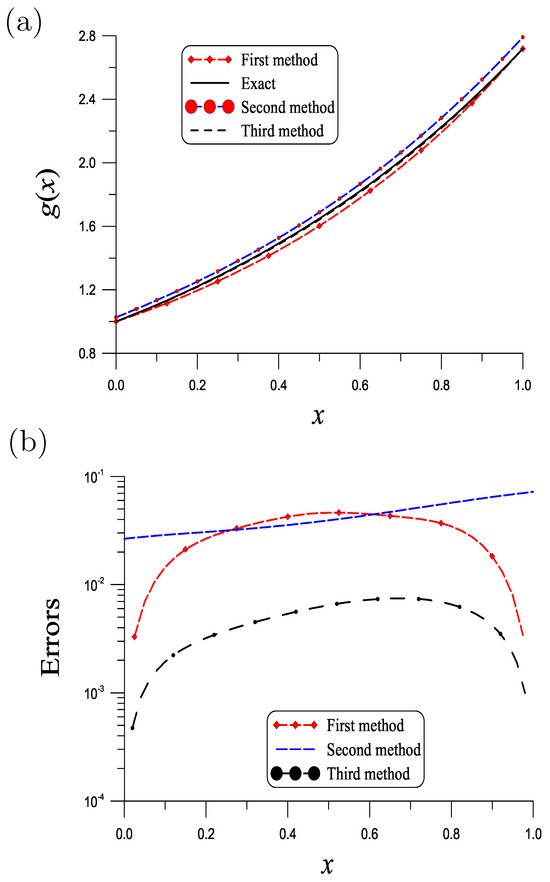
Example 5.

We take Example 1 again,

$$v(x,t)=e^{-t}sinx,g\left(x\right)=sinx.$$

(62)

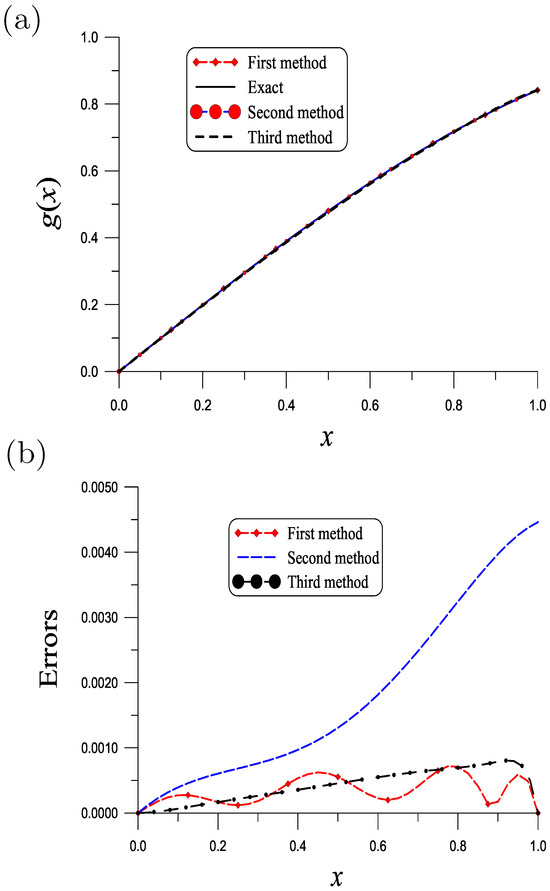
With $s=2\%$, $m=5$, $\alpha =0.2$, $t_f=0.6$ and $N_1=41$, good result is obtained by the first method as shown in Figure 4a. The ME over the unit interval $[0,1]$ is $7.16\times {10}^{-4}$ as shown in Figure 4b. Under the same values of parameters, the result obtained by the second method is shown in Figure 4a, whose ME is $4.46\times {10}^{-3}$ as shown in Figure 4b. The ME rendered by the third method with $m_1=10$ and $m_2=6$ is $8.05\times {10}^{-4}$ as shown in Figure 4b. The CPU times for the first, second and third methods are, respectively, 8.69 s, 1.56 s and 0.67 s.

Figure 4. (a) Comparing recovered and exact initial temperatures for Example 5, and (b) numerical errors.

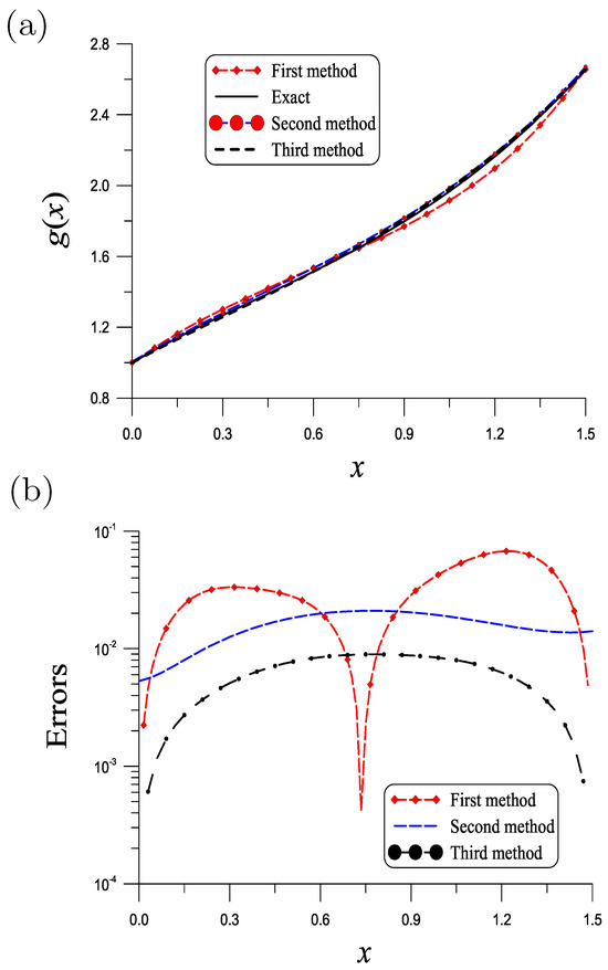
Example 6.

Consider

$$v(x,t)=e^{x+t}cos\left(xt\right),g\left(x\right)=e^x.$$

(63)

By $s=10\%$, $m=5$, $\alpha =0.9$, $t_f=0.2$ and $N_1=41$, good result is obtained by the first method as shown in Figure 5a. ME is $4.63\times {10}^{-2}$ as shown in Figure 5b. The result obtained by the second method is shown in Figure 5a; ME = $7.21\times {10}^{-2}$ is seen from Figure 5b. The ME rendered by the third method with $m_1=m_2=3$ is $8.48\times {10}^{-3}$ as shown in Figure 5b. The CPU times for the first, second and third methods are, respectively, 5.74 s, 0.67 s and 0.34 s.

Figure 5. (a) Comparing recovered and exact initial temperatures for Example 6, and (b) numerical errors.

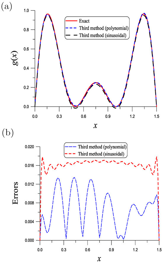
Example 7.

A more complex initial temperature is considered:

$$v(x,t)=e^{-t^2}(x{e}^{-x}+x^2+cosx),g\left(x\right)=x{e}^{-x}+x^2+cosx.$$

(64)

By $s=2\%$, $m=6$, $\alpha =0.6$, $t_f=0.1$ and $N_1=101$, good result is obtained by the first method as shown in Figure 6a. ME over $[0,1.5]$ is $6.75\times {10}^{-2}$ as shown in Figure 6b. The result obtained by the second method is shown in Figure 6a, whose ME = $2.1\times {10}^{-2}$ is seen from Figure 6b. ME = $8.95\times {10}^{-3}$ is obtained by the third method with $m_1=10$ and $m_2=2$ as shown in Figure 6b. The CPU times for the first, second and third methods are, respectively, 2.51 s, 0.39 s and 0.21 s.

Figure 6. (a) Comparing recovered and exact initial temperatures for Example 7, and (b) numerical errors.

Example 8.

For further testing the performance of the third method, we consider

$$u(x,t)=t^{2}sin\left(\pi x\right),g\left(x\right)=0,S(x,t)=\left[\frac{\Gamma \left(3\right)}{\Gamma (3-\alpha )}{t}^{2-\alpha }+{\pi }^2{t}^2\right]sin\left(\pi x\right).$$

(65)

Table 2 lists the ME for the recovery of $g\left(x\right)$ rendered by the third method with $m_1=4$ and $m_2=2$. We fix $s=2\%$, $\alpha =0.7$, $a=1$, and vary $t_f$. Good results are obtained. It can be seen that all MEs are much smaller than the error of noise with $s=0.02$.

Table 2. For Example 8, solved by the third method, listing the MEs of $g\left(x\right)$.

${\mathit{t}}_{\mathit{f}}$	0.2	0.5	0.8	1	1.5	2	3
ME	$1.47\times {10}^{-5}$	$5.77\times {10}^{-5}$	$9.97\times {10}^{-5}$	$1.27\times {10}^{-4}$	$1.98\times {10}^{-4}$	$2.69\times {10}^{-4}$	$4.19\times {10}^{-4}$

Example 9.

We apply the third method to a large time span and a high noisy case:

$$\begin{array}{c}u(x,t)=t+(1-2x)(2-2x)sin\left(2\pi x\right),g\left(x\right)=(1-2x)(2-2x)sin\left(2\pi x\right),\hfill \\ S(x,t)=\frac{t^{1-\alpha }}{\Gamma (2-\alpha )}-g^{\prime \prime }\left(x\right).\hfill \end{array}$$

(66)

For $s=10\%$, $m_1=15$, $m_2=3$, $\alpha =0.25$, $a=1.5$, and $t_f=5$, shown in Figure 7a is a good recovery of the initial temperature with a large time duration and under a large noise. ME over $[0,1.5]$ shown in Figure 7b is $1.34\times {10}^{-2}$.

Figure 7. (a) Comparing recovered and exact initial temperatures for Example 9, and (b) numerical errors.

In addition to Equation (58), the following bases can also be adopted:

$$B^{jk}(x,t)=sin\left(\frac{j\pi x}{a}\right)\left[{\left(\frac{t}{t_f}\right)}^k-1\right]\in G.$$

(67)

We solve this example again by using this sinusoidal bases. We raise $m_1$ to $m_1=25$ and other parameters values are the same. ME over $[0,1.5]$ shown in Figure 7b is $1.78\times {10}^{-2}$, which is slightly larger than that using the polynomial bases in Equation (58).

Example 10.

To compare the result obtained in [41], we take

$$\begin{array}{c}{D}_t^{\alpha }u(x,t)=u_{xx}(x,t),(x,t)\in (0,\pi )\times (0,t_f],\hfill \\ u(0,t)=u(\pi ,t)=0,u(x,0)=sinx+sin2x,\hfill \\ u(x,t)=E_{1/2,1}(-t^{1/2})sinx+E_{1/2,1}(-4t^{1/2})sin2x,\hfill \end{array}$$

(68)

where the function $E_{1/2,1}\left(s\right)$ is given by

$$E_{1/2,1}\left(s\right)=\frac{2}{\sqrt{\pi }}{e}^{s^2}{\int }_{-s}^{\infty }{e}^{-{\tau }^2}d\tau .$$

(69)

The absolute noise δ is imposed on the final time data by

$$\widehat{f}\left(x\right)=u(x,t_f)+\sqrt{\frac{2}{\pi }}\delta R\left(x\right).$$

(70)

For $\delta =0.032$, the $L^2$ error obtained in [41] is 1.5415. By $m=3$ the second method obtains 0.55203 of the $L^2$ error. With $m_1=2$, $m_2=4$, $\alpha =0.5$, $a=\pi$, and $t_f=1$, we recover the initial temperature with $B^{jk}(x,t)$ given by Equation (67). The $L^2$ error obtained by the third method is 0.89075, which is smaller than 1.5415 obtained in [41]. Moreover, the $L^2$ error 0.55203 obtained by the second method is smaller than 0.89075 obtained by the third method, and much smaller than 1.5415 obtained in [41].

7. Conclusions

In this paper we have transformed the inverse source problem to recover the space-time dependent source functions of a time-fractional diffusion equation into a problem by using a symmetry boundary functions method to find the solution. Four examples confirmed the efficiency and accuracy of the presented method. Then, three novel methods were developed to solve the backward problems of the time-fractional diffusion equations. We first transformed the unknown initial temperature problem into a space-dependent inverse source problem for a new variable. Then, the initial temperature can be recovered by using the energetic boundary functions as the bases and solving a second-order boundary value problem. In the second method, the energetic boundary functions were used as the bases and then collocated to a linear system to obtain the whole solution. In the first and second methods, the initial temperature was recovered by over-specifying boundary fluxes and giving no final time condition. In the third method, two boundary conditions and a final time temperature were used to construct the bases resorting on the group symmetry. Then, the governing equation was collocated to a linear system to obtain the whole solution. These three methods were compared by numerical testings. Among them, the third method to treat the standard backward time-fractional diffusion problem is the simplest one, whose accuracy is excellent; the third method spent less CPU time than other two methods.

The main achievements involved in the paper are as follows:

• Introduced the group symmetry boundary functions methods for solving the inverse source and backward problems of time-fractional diffusion equations.
• Owing to good properties of the boundary functions, we can solve the inverse problems with a few bases such that without using the regularization technique to obtain good results.
• We developed three novel group symmetry methods to solve the backward time-fractional diffusion problems to achieve an accurate recovery of the initial temperature, which spent a little CPU time and were robust against large noise.

References

- Gu, Y.T.; Zhuang, P.; Liu, F. An advanced implicit meshless approach for the non-linear anomalous subdiffusion equation. Comput. Model. Eng. Sci. 2010, 56, 303–333. [Google Scholar]
- Gorenflo, R.; Mainardi, F. Random walk models for space fractional diffusion processes. Fract. Calc. Appl. Anal. 1998, 1, 167–191. [Google Scholar]
- Metzler, R.; Klafter, J. The restaurant at the end of the random walk: Recent developments in the description of anomalous transport by fractional dynamics. J. Phys. A Math. Gen. 2004, 37, 161–208. [Google Scholar] [CrossRef]
- Ye, H.; Ding, Y. Dynamical analysis of a fractional-order HIV model. Comput. Model. Eng. Sci. 2009, 49, 255–268. [Google Scholar]
- Kou, C.; Yan, Y.; Liu, J. Stability analysis for fractional differential equations and their applications in the models of HIV-1 infection. Comput. Model. Eng. Sci. 2009, 39, 301–318. [Google Scholar]
- Sivaprasad, R.; Venkatesha, S.; Manohar, C.S. Identification of dynamical systems with fractional derivative damping models using inverse sensitivity analysis. Comput. Mater. Contin. 2009, 9, 179–208. [Google Scholar]
- Caputo, M. Linear models of dissipation whose Q is almost frequency independent, II. Geophys. J. R. Astron. Soc. 1967, 13, 529–539. [Google Scholar] [CrossRef]
- Caputo, M.; Mainardi, F. A new dissipation model based on memory mechanism. Pure Appl. Geophys. 1971, 91, 134–147. [Google Scholar] [CrossRef]
- Liu, C.S. The fictitious time integration method to solve the space- and time-fractional Burgers equations. Comput. Mater. Contin. 2010, 15, 221–240. [Google Scholar]
- Kirane, M.; Malik, A.S. Determination of an unknown source term and the temperature distribution for the linear heat equation involving fractional derivative in time. Appl. Math. Comput. 2011, 218, 163–170. [Google Scholar] [CrossRef][Green Version]
- Jin, B.; Rundell, W. An inverse problem for a one-dimensional time-fractional diffusion problem. Inv. Prob. 2012, 28, 075010. [Google Scholar] [CrossRef]
- Wang, J.G.; Zhou, Y.B.; Wei, T. Two regularization methods to identify a space-dependent source for the time-fractional diffusion equation. Appl. Numer. Math. 2013, 68, 39–57. [Google Scholar] [CrossRef]
- Zhang, Z.Q.; Wei, T. Identifying an unknown source in time-fractional diffusion equation by a truncation method. Appl. Math. Comput. 2013, 219, 5972–5983. [Google Scholar] [CrossRef]
- Wei, T.; Wang, J. A modified quasi-boundary value method for an inverse source problem of the time-fractional diffusion equation. Appl. Numer. Math. 2014, 78, 95–111. [Google Scholar] [CrossRef]
- Tuan, N.H.; Long, L.D.; Nguyen, V.T. Regularized solution of an inverse source problem for a time fractional diffusion equation. Appl. Math. Model. 2016, 40, 8244–8264. [Google Scholar]
- Tuan, N.H.; Nane, E. Inverse source problem for time-fractional diffusion with discrete random noise. Stat. Prob. Lett. 2017, 120, 126–134. [Google Scholar] [CrossRef]
- Ruan, Z.; Wang, Z. Identification of a time-dependent source term for a time fractional diffusion problem. Appl. Anal. 2017, 96, 1638–1655. [Google Scholar] [CrossRef]
- Sun, H.G.; Chang, A.; Zhang, Y.; Chen, W. A review on variable-order fractional differential equations: Mathematical foundations, physical models, numerical methods and applications. Frac. Calc. Appl. Anal. 2019, 22, 27–59. [Google Scholar] [CrossRef]
- Li, H.; Wu, Y. Artificial boundary conditions for nonlinear time fractional Burgers’ equation on unbounded domains. Appl. Math. Lett. 2021, 120, 107277. [Google Scholar] [CrossRef]
- Chen, L.; Lü, S.; Xu, T. Fourier spectral approximation for time fractional Burgers equation with nonsmooth solutions. Appl. Numer. Math. 2021, 169, 164–178. [Google Scholar] [CrossRef]
- Li, C.; Li, D.; Wang, Z. L1/LDG method for the generalized time-fractional Burgers equation. Math. Comput. Simul. 2021, 187, 357–378. [Google Scholar] [CrossRef]
- Ali, I.; Haq, S.; Aldosary, S.F.; Nisar, K.S.; Ahmad, F. Numerical solution of one- and two-dimensional time-fractional Burgers equation via Lucas polynomials coupled with Finite difference method. Alex. Eng. J. 2022, 61, 6077–6087. [Google Scholar] [CrossRef]
- Zhang, Q.; Sun, C.; Fang, Z.-W.; Sun, H.-W. Pointwise error estimate and stability analysis of fourth-order compact difference scheme for time-fractional Burgers’ equation. Appl. Math. Comput. 2022, 418, 126824. [Google Scholar] [CrossRef]
- Qiao, L.; Tang, B. An accurate, robust, and efficient finite difference scheme with graded meshes for the time-fractional Burgers’ equation. Appl. Math. Lett. 2022, 128, 107908. [Google Scholar] [CrossRef]
- Shen, J.-Y.; Ren, J.; Chen, S. A second-order energy stable and nonuniform time-stepping scheme for time fractional Burgers’ equation. Comput. Math. Appl. 2022, 123, 227–240. [Google Scholar] [CrossRef]
- Singh, B.K.; Gupta, M. Trigonometric tension B-spline collocation approximations for time fractional Burgers’ equation. J. Ocean Eng. Sci. 2022, in press. [CrossRef]
- Shafiq, M.; Abbas, M.; Abdullah, F.A.; Majeed, A.; Abdeljawad, T.; Alqudah, M.A. Numerical solutions of time fractional Burgers’ equation involving Atangana–Baleanu derivative via cubic B-spline functions. Results Phys. 2022, 34, 105244. [Google Scholar] [CrossRef]
- Zhang, Y.; Feng, M. A local projection stabilization virtual element method for the time-fractional Burgers equation with high Reynolds numbers. Appl. Math. Comput. 2023, 436, 127509. [Google Scholar] [CrossRef]
- Peng, X.; Xu, D.; Qiu, W. Pointwise error estimates of compact difference scheme for mixed-type time-fractional Burgers’ equation. Math. Comput. Simul. 2023, 208, 702–726. [Google Scholar] [CrossRef]
- Elbadri, M. An approximate solution of a time fractional Burgers’ equation involving the Caputo-Katugampola fractional derivative. Partial Differ. Equ. Appl. Math. 2023, 8, 100560. [Google Scholar] [CrossRef]
- Wang, Y.; Sun, T. Two linear finite difference schemes based on exponential basis for two-dimensional time fractional Burgers equation. Physica D 2024, 459, 134024. [Google Scholar] [CrossRef]
- Liaqat, M.I.; Akgül, A. A novel approach for solving linear and nonlinear time-fractional Schrödinger equations. Chaos Solit. Fractals 2022, 162, 112487. [Google Scholar] [CrossRef]
- Wang, F.; Salama, S.A.; Khater, M.M.A. Optical wave solutions of perturbed time-fractional nonlinear Schrödinger equation. J. Ocean Eng. Sci. 2022, in press. [CrossRef]
- Ameen, I.G.; Ahmed Taie, R.O.; Ali, H.M. Two effective methods for solving nonlinear coupled time-fractional Schrödinger equations. Alex. Eng. J. 2023, 70, 331–347. [Google Scholar] [CrossRef]
- Kopcasiz, B.; Yaşar, E. Adaptation of Caputo residual power series scheme in solving nonlinear time fractional Schrödinger equations. Optik 2023, 289, 171254. [Google Scholar] [CrossRef]
- Devnath, S.; Khan, K.; Akbar, M.A. Numerous analytical wave solutions to the time-fractional unstable nonlinear Schrödinger equation with beta derivative. Partial Differ. Equ. Appl. Math. 2023, 8, 100537. [Google Scholar] [CrossRef]
- Liu, J.J.; Yamamoto, M. A backward problem for the time-fractional diffusion equation. Appl. Anal. 2010, 89, 1769–1788. [Google Scholar] [CrossRef]
- Tuan, N.H.; Long, L.D.; Nguyen, V.T. Tikhonov regularization method for a backward problem for the inhomogeneous time-fractional diffusion equation. Appl. Anal. 2016, 97, 842–863. [Google Scholar] [CrossRef]
- Tuan, N.H.; Long, L.D.; Nguyen, V.T.; Tran, H. On a final value problem for the time-fractional diffusion equation with inhomogeneous source. Inv. Prob. Sci. Eng. 2016, 25, 1367–1395. [Google Scholar] [CrossRef]
- Al-Jamal, M.F. A backward problem for the time-fractional diffusion equation. Math. Meth. Appl. Sci. 2017, 40, 2466–2474. [Google Scholar] [CrossRef]
- Hào, D.N.; Liu, J.; Duc, N.V.; Thang, N.V. Stability results for backward time-fractional parabolic equations. Inv. Prob. 2019, 35, 125006. [Google Scholar]
- Li, Y.; Zhang, H. Landweber iterative regularization method for an inverse initial value problem of diffusion equation with local and nonlocal operators. Appl. Math. Sci. Eng. 2023, 31, 2194644. [Google Scholar] [CrossRef]
- Podlubny, I. Fractional Differential Equations; Academic Press: San Diego, CA, USA, 1999. [Google Scholar]
- Samko, S.G.; Kilbas, A.A.; Marichev, O.I. Fractional Integrals and Derivatives: Theory and Applications; Gordon and Breach Science: New York, NY, USA, 1987. [Google Scholar]
- Langlands, T.A.M.; Henry, B.I. The accuracy and stability of an implicit solution method for the fractional diffusion equation. J. Comput. Phys. 2005, 205, 719–736. [Google Scholar] [CrossRef]
- Lin, Y.; Xu, C. Finite difference/spectral approximations for the time-fractional diffusion equation. J. Comput. Phys. 2007, 225, 1533–1552. [Google Scholar] [CrossRef]
- Lin, Y.; Li, X.; Xu, C. Finite difference/spectral approximations for the fractional cable equation. Math. Comput. 2011, 80, 1369–1396. [Google Scholar] [CrossRef]
- Zeng, F.; Li, C.; Liu, F.; Turner, I. The use of finite difference/element approaches for solving the time-fractional subdiffusion equation. SIAM J. Sci. Comput. 2013, 35, A2976–A3000. [Google Scholar] [CrossRef]
- Diethelm, K. An algorithm for the numerical solution of differential equations of fractional order. Electron. Trans. Numer. Anal. 1997, 5, 1–6. [Google Scholar]
- Ford, N.J.; Xiao, J.; Yan, Y. A finite element method for time fractional partial differential equations. Fract. Calc. Appl. Anal. 2011, 14, 454–474. [Google Scholar] [CrossRef]
- Li, Z.; Liang, Z.; Yan, Y. High-order numerical methods for solving time fractional partial differential equations. J. Sci. Comput. 2017, 71, 785–803. [Google Scholar] [CrossRef]
- Alperin, J.L.; Bell, R.B. Groups and Representations; Springer: New York, NY, USA, 1995. [Google Scholar]
Disclaimer/Publisher’s Note: The statements, opinions and data contained in all publications are solely those of the individual author(s) and contributor(s) and not of MDPI and/or the editor(s). MDPI and/or the editor(s) disclaim responsibility for any injury to people or property resulting from any ideas, methods, instructions or products referred to in the content. |
© 2024 by the authors. Licensee MDPI, Basel, Switzerland. This article is an open access article distributed under the terms and conditions of the Creative Commons Attribution (CC BY) license (https://creativecommons.org/licenses/by/4.0/).