A Gradient-Based Algorithm with Nonmonotone Line Search for Nonnegative Matrix Factorization

Abstract

In this paper, we first develop an active set identification technique, and then we suggest a modified nonmonotone line search rule, in which a new parameter formula is introduced to control the degree of the nonmonotonicity of line search. By using the modified line search and the active set identification technique, we propose a global convergent method to solve the NMF based on the alternating nonnegative least squares framework. In addition, the larger step size technique is exploited to accelerate convergence. Finally, a large number of numerical experiments are carried out on synthetic and image datasets, and the results show that our presented method is effective in calculating speed and solution quality.

1. Introduction

As a typical nonnegative data dimensionality reduction technology, nonnegative matrix factorization (NMF) [1,2,3,4,5] can efficiently mine hidden information from data, so it has been gradually applied to research into high-dimensional data. This method as a data reduction technique appears in many applications, such as image processing [2], text mining [6], blind source separation [7], clustering [8], music analysis [9], and hyperspectral imaging unmixing [10], to name a few. Generally speaking, the fundamental NMF problem can be summarized as follows: given an $m\times n$ data matrix $V=\left(V_{ij}\right)$ with $V_{ij}\ge 0$ and a predetermined positive integer $r<min(m,n)$, then NMF plans to find two nonnegative matrices $W\in {\mathbb{R}}_{+}^{m\times r}$ and $H\in {\mathbb{R}}_{+}^{r\times n}$ such that

$$\begin{array}{c}\hfill V\approx WH.\end{array}$$

(1)

Our visualization illustration of NMF is shown in Figure 1.

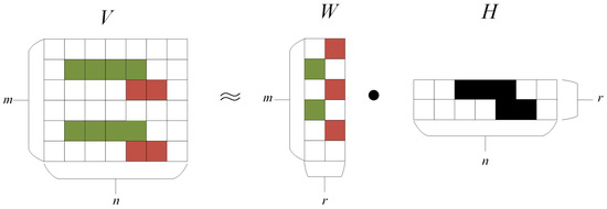
Figure 1. Visualization illustration of NMF.

One of the most commonly used models of NMF (1) is

$$\begin{array}{c}\hfill \begin{array}{c}\hfill {\displaystyle \underset{W,H}{min}f(W,H)\equiv \frac{1}{2}{\parallel V-WH\parallel }_F^2}\hfill \\ \hfill {\displaystyle \mathrm{subject}\mathrm{to}W\ge 0,H\ge 0.}\hfill \end{array}\end{array}$$

(2)

where ${\parallel ·\parallel }_F$ is the Frobenius norm.

The project Barzilai-Borwein (PBB) algorithm is regarded as a popular and effective method for solving (2) which was originated by Barzilai and Borwein [11]. In recent years, a large number of studies [12,13,14,15,16] have shown that the PBB algorithm is a very effective algorithm in solving optimal problems. The PBB algorithm has the characteristics of simple calculation and high efficiency, so it has been paid attention to by various disciplines. So far, the research results based on the PBB have been widely used in the field of NMF (see [17,18,19,20,21]).

In view of the perfect symmetry of the interaction between W and H, we will focus on the updating of matrix W based on the PBB algorithm. Remember that $H^k$ is an approximate value of H after kth update, and there are

$$\begin{array}{c}\hfill {\displaystyle f(W,H^k)=\frac{1}{2}{\parallel V-W{H}^k\parallel }_F^2\forall k.}\end{array}$$

(3)

At each step for solving (3), there are three different updates:

$$W^{k+1}=\underset{W\ge 0}{min}f(W,H^k);$$

(4)

$$W^{k+1}=\underset{W\ge 0}{min}f(W,H^k)+⟨\nabla f\left(W\right),W-W^k⟩+\frac{L_W^k}{2}{\parallel W-W^k\parallel }_F^2;$$

(5)

$$W^{k+1}=\underset{W\ge 0}{min}⟨\nabla f\left(W^k\right),W-W^k⟩+\frac{L_W^k}{2}{\parallel W-W^k\parallel }_F^2,$$

(6)

where $L_W^k>0$, $\nabla f\left(W\right)={\nabla }_{W}f(W,H^k)$.

Original cost function (4) is the most frequently used form in the PBB method for NMF and has been widely and deeply researched [17,20,21,22,23]. But the major disadvantage of (4) is that it is not strongly convex [24,25,26,27,28], and we can only hope that this method can find a stationary point, rather than a global or local minimizer. To overcome this drawback, a proximal modification of cost function (4) is presented in [18,19], namely, the proximal cost function (5).

At present, the proximal cost function (5) has been used with the PBB method for NMF in [18,19]. When the cost function (5) is a strongly convex quadratic optimization problem, their lower bound is zero, so the subproblem (5) has a unique minimizer. In [18], the authors present a quadratic regularization nonmonotone PBB algorithm to solve (5) and established its global convergence result under mild conditions. Recently, it is revisited in [19] for the monotone PBB method and is also shown to converge globally to a stationary point of (3), and through the analysis of numerical experiments, it is proved that the monotone PBB method can win over the nonmonotone one under certain conditions. However, when solving the problems (4) and (5), the existing gradient methods based on the PBB converge slowly due to the nonnegative conditions. Therefore, this project intends to develop a new fast NMF algorithm.

In this paper, we introduce a prox-linear approximation of $f(W,H^k)$ at $W^k$ based on $\nabla f\left(W\right)$ which is the cost function (6). And then we propose an active set identification technique. Next, we present a modified nonmonotone line search technique so as to improve the efficiency of nonmonotone line search, in which a new parameter formula is presented to attempt to control the degree of the nonmonotonicity of line search, and thus improve both the possibility of finding the global optimal solution and the convergence speed. By using the active set identification strategy and the modified nonmonotone line search, a global convergent method is proposed to solve (6) based on the alternating nonnegative least squares framework. In particular, in each iteration, identification techniques are used to determine active and free variables. We take ${\left(D_t\right)}_{ij}=0$ or ${\left(D_t\right)}_{ij}=-{\left(Z_t\right)}_{ij}$ to update some active variables, while using a projected Barzilai-Borwein method to update the free variables and some active variables. The calculation speed is improved by using the method of larger step size. Finally, through the numerical experiments of simulation data and image data, it is proved that the proposed algorithm is effective.

This paper is organized in the following manner. In Section 3, we introduce our estimation of active set, put forward an efficient NMF algorithm, and present the global convergence results of this method. The experimental results are given in Section 4. Finally, Section 5 is the conclusion of the thesis.

2. A Fast PBB Algorithm

In this section, we present an efficient algorithm for solving the NMF and establish the global convergence of our algorithm. Now, let us first introduce some main results of the objective function $f(W,H^k)$ that we know.

Lemma 1 

([29]). The following two statements are valid.

(i)

The objective function $f(W,H^k)$ of (3) is convex.

(ii)

The gradient

$$\begin{array}{c}\hfill {\nabla }_{W}f(W,H^k)=(W{H}^k-V){\left(H^k\right)}^T\end{array}$$

is Lipschitz continuous with the constant $L_W={\parallel H^k{\left(H^k\right)}^T\parallel }_2$.

In order to facilitate the discussion, we mainly focus on (6) and then rewrite it. Note that the cost function (7) is closely related to the one in Xu et al. [30], but has the following difference: matrix U is $W_t$ in our cost function (7), however, to [30] the matrix U is an extrapolation point in $W_t$.

$$\begin{array}{c}\hfill \underset{W\ge 0}{min}\phi (U,W):=⟨\nabla f\left(U\right),W-U⟩+\frac{L_W}{2}{\parallel W-U\parallel }_F^2,\end{array}$$

(7)

where the fixed matrix $U\ge 0$.

According to (ii) of the Lemma 1, $\phi (U,W)$ is strictly convex in W for any given U. In each iteration, we will first solve the following strongly convex quadratic minimization problem, so as to obtain a $Z_t$ value

$$\begin{array}{c}\hfill \underset{W\ge 0}{min}\phi (W_t,W).\end{array}$$

(8)

Because the objective function of the problem (8) is strongly convex, the solution of the problem is unique and closed-form

$$\begin{array}{c}\hfill Z_t=P[W_t-\frac{1}{L_W}{\nabla }_{W}f(W_t,H^k)],\end{array}$$

(9)

Here, the operator $P\left[X\right]$ projects all negative terms of X to zero.

Let $W_{t+1}=Z_t+D_t$, where $D_t$ is the direction which is obtained by (23) with ${\alpha }_t$ being the BB stepsize [11], whereby we see that the convergence of $\left\{W_{t+1}\right\}$ can not be guaranteed. Therefore, a global optimization strategy is proposed based on the modified Armiji line search [31].

Therefore, a globalization strategy based on the modified Armiji line search [31] has been proposed, that is, we ask for a step size ${\lambda }_t$, so that

$$f(Z_t+{\lambda }_t{D}_t)\le \underset{0\le j\le min\{t,M-1\}}{max}f\left(Z_{t-j}\right)+\gamma {\lambda }_t⟨\nabla f\left(Z_t\right),D_t⟩,$$

(10)

here $M>0$. Owing to the maximum function, a good function value obtained in any iteration will be discarded, and the numerical performance depends largely on the selection of M in some cases (see [32]).

So as to overcome these shortcomings and obtain a large step size in each procedure, we present a modified nonmonotone line search rule. The modified line search is as follows: for the known iteration point $Z_t$ and search direction $D_t$ at $Z_t$, we select ${\eta }_t\in [{\eta }_{min},{\eta }_{max}]$, where $0<{\eta }_{min}<{\eta }_{max}<1$, ${\gamma }_t\in [{\gamma }_{min},{\gamma }_{max}(1-{\eta }_{max})]$, where ${\gamma }_{max}<1$, $0<{\gamma }_{min}<(1-{\eta }_{max}){\gamma }_{max}$, $0\le \mu \le 1$, and $s>1$, to find a ${\lambda }_t$ satisfying the following inequality:

$$\begin{array}{c}\hfill \begin{array}{c}\hfill S_{t+1}\le S_t+{\gamma }_t{\lambda }_t[⟨\nabla f\left(Z_t\right),D_t⟩+\frac{\mu }{{\alpha }_t}\parallel D_t{\parallel }^2],\end{array}\end{array}$$

(11)

where $S_t$ is defined as

$$\begin{array}{c}\hfill S_t=\left\{\begin{array}{cc}f\left(W_0\right),\hfill & \mathrm{if}t=0,\hfill \\ f\left(W_t\right)+{\eta }_{t-1}(S_{t-1}-f\left(W_t\right)),\hfill & \mathrm{if}t\ge 1,\hfill \end{array}\right.\end{array}$$

(12)

Similar to M in (10), the selection ${\eta }_t$ in (12) is an important factor in determining the degree of nonmonotonicity (see [33]). Thus, to improve the efficiency of a nonmonotone line search, Ahookhosh et al. [34] choose a varying value for the parameter ${\eta }_t$ by using a simple formula. Later, Nosratipour et al. [35] decided that ${\eta }_t$ should be related to a suitable criterion to measure the distance to the optimal solution. Thus, they defined ${\eta }_t$ by

$$\begin{array}{c}\hfill {\eta }_t=1-e^{-\parallel \nabla f\left(Z_t\right)\parallel }.\end{array}$$

(13)

However, we found that if the iterative sequence $\left\{Z_t\right\}$ is trapped in a narrow curved valley, then it can lead to $\nabla f\left(Z_t\right)=0$, from which we can obtain ${\eta }_t=0$, so the nonmonotone line search is reduced to the standard Armijo line search, which is inefficient owing to the generation of very short or zigzagging steps. To overcome this drawback, we suggest the following ${\eta }_t$:

$$\begin{array}{c}\hfill {\eta }_t=\frac{2}{\pi }arctan\left(\right|f\left(Z_t\right)-f\left(Z_{t-1}\right)\left|\right).\end{array}$$

(14)

It is obvious that $|f\left(Z_t\right)-f\left(Z_{t-1}\right)|$ is large when the function value decreases rapidly, and then ${\eta }_t$ will also be large, so therefore the nonmonotone strategy will be stronger. However, when $f\left(Z_t\right)$ is close to the optimal solution, we can obtain $|f\left(Z_t\right)-f\left(Z_{t-1}\right)|$ which tends toward zero, and then ${\eta }_t$ also tends toward zero, so then the nonmonotone rule will be weaker and it tends to be a monotone rule.

As was observed in [16], the active set method can enhance the efficiency of the local convergence algorithm and reduce the computing cost. There-in-after, we will recommend an active set recognition technology to approximate the right sustain of the solution points. In our context, we deal with the active set which is considered as the subset of zero components of $Z^{*}$. Now, we introduce the active set L as the index set corresponding to the zero component. Meanwhile, the inactive set F is to be the support of $Z^{*}$.

Definition 1. 

Let $\mathrm{\Omega }=\{Z\in {\mathbb{R}}^{m\times r}:Z\ge 0\}$ and $Z^{*}$ be a stationary point of (3). We define the active set as follows:

$$\begin{array}{c}\hfill L=\{ij:Z_{ij}^{*}=0\},\end{array}$$

(15)

We further define an inactive set F which is a complementary set of L,

$$\begin{array}{c}\hfill F\left(Z\right)=I\backslash L\left(Z\right),\end{array}$$

(16)

where $I=\{11,12,\dots ,1r,21,22,\dots ,2r,\dots ,m1,m2,\dots ,mr\}$.

Then, for any $\left(Z_t\right)\in \mathrm{\Omega }$, we define the following approximations $L\left(Z_t\right)$ and $F\left(Z_t\right)$ as $\overline{L}$ and $\overline{F}$, respectively,

$$\begin{array}{ccc}& & \hfill L\left(Z_t\right)=\{ij:{\left(Z_t\right)}_{ij}\le \frac{1}{{\alpha }_t}\nabla f{\left(Z_t\right)}_{ij}\},\hfill \end{array}$$

(17)

$$\begin{array}{ccc}& & \hfill F\left(Z_t\right)=I\backslash L\left(Z_t\right),\hfill \end{array}$$

(18)

where ${\alpha }_t$ is the BB step size. For simplicity, we abbreviate $L\left(Z_t\right)$ and $F\left(Z_t\right)$ as $L_t$ and $F_t$, respectively. Similar to the Lemma 1 in [21], we have that if the strict complementarity is satisfied at $Z_t$, then $L\left(Z_t\right)$ coincides with the active set if $Z_t$ is sufficiently close to $Z^{*}$.

In order to obtain a well estimate of the active set, the active set is further subdivided into two sets

$$\begin{array}{c}\hfill L_1\left(Z_t\right)=\{ij\in L\left(Z_t\right):\nabla f{\left(Z_t\right)}_{ij}\ge c\},\end{array}$$

(19)

and

$$\begin{array}{c}\hfill L_2\left(Z_t\right)=\{ij\in L\left(Z_t\right):\nabla f{\left(Z_t\right)}_{ij}<c\},\end{array}$$

(20)

here $c>0$ is a constant.

Obviously, $L_2\left(Z_t\right)$ is the index set of variables with the first-order necessary condition. Therefore, we have reason to set the variables with indices in $L_2\left(Z_t\right)$ to 0. In addition, because $L_1\left(Z_t\right)$ is an index set that does not satisfy the first-order necessary condition, we further subdivide $L_1\left(Z_t\right)$ into two subsets

$$\begin{array}{c}\hfill {\overline{L}}_1\left(Z_t\right)=\{ij:ij\in L_1\left(Z_t\right)\mathrm{and}{\left(Z_t\right)}_{ij}=0\},\end{array}$$

(21)

and

$$\begin{array}{c}\hfill {\tilde{L}}_1\left(Z_t\right)=\{ij:ij\in L_1\left(Z_t\right)\mathrm{and}{\left(Z_t\right)}_{ij}\ne 0\}.\end{array}$$

(22)

When a variable is with indices in ${\overline{L}}_1\left(Z_t\right)$, we consider the direction of the form 0. And for the variables of the indexs in ${\tilde{L}}_1\left(Z_t\right)$, we consider the direction of the form $-Z_t$, so as to to improve the corresponding components. Thus, through the above discussion, we define this direction in the following compact form:

$${\left(D_t\right)}_{ij}=\left\{\begin{array}{cc}0,\hfill & \mathrm{if}ij\in {\overline{L}}_1\left(Z_t\right),\hfill \\ -{\left(Z_t\right)}_{ij},\hfill & \mathrm{if}ij\in {\tilde{L}}_1\left(Z_t\right),\hfill \\ {(P[Z_t-{\alpha }_t\nabla f\left(Z_t\right)]-Z_t)}_{ij},\hfill & \mathrm{if}ij\in L_2\left(Z_t\right)\cup F\left(Z_t\right),\hfill \end{array}\right.$$

(23)

where ${\alpha }_t$ is the BB stepsize.

Finally, we let

$$\begin{array}{c}\hfill W_{t+1}=Z_t+{\lambda }_t{D}_t,\end{array}$$

(24)

where ${\lambda }_t$ is the step size which is found by using a nonmonotonic line search (11).

It is known from [36] that the larger step size technique can significantly accelerate the rate of convergence of the algorithm, so by adding a relaxation factor s to the update rule of $W_{t+1}$ (24), we modify the update rule (24) as

$$W_{t+1}=Z_t+s{\lambda }_t{D}_t$$

(25)

for relaxation factor $s>1$. We show that the optimal parameter s in (25) is $s=1.7$ by number experiments in Section 4.4.

Based on the above discussion, we develop a nonmonotone projected Barzilai-Borwein method based on the active set strategy proposed in Section 3 and outline the proposed algorithm in Algorithm 1. We can follow a similar procedure for updating H.

Algorithm 1 Nonmonotone projected Barzilai-Borwein algorithm (NMPBB).

Initialize ${\alpha }_0=1$, ${\eta }_t\in (0,1)$, choose parameters ${\eta }_t\in [{\eta }_{min},{\eta }_{max}]$, ${\gamma }_t\in [{\gamma }_{min},{\gamma }_{max}(1-{\eta }_{max})]$, ${\alpha }_{max}>{\alpha }_{min}>0$, $\mu \in [0,1],\rho \in (0,1)$, $s>1$, $L_W={\parallel H^k{\left(H^k\right)}^T\parallel }_2$ and $W_0=W^k$. Set $t=0$. If $\parallel P[W_t-\nabla f\left(W_t\right)]-W_t\parallel =0$, stop. Compute $Z_t=P[W_t-\frac{1}{L_W}\nabla f(W_t,H^k)]$. Compute $S_t$ by (12) and compute $D_t$ by (23). Nonmonotone line search. Let $m_t$ be the smallest nonnegative integer m satisfying $$\begin{array}{c}\hfill S_{t+1}\le S_t+{\gamma }_t{\rho }^m[⟨\nabla f\left(Z_t\right),D_t⟩+\frac{\mu }{{\alpha }_t}\parallel D_t{\parallel }^2],\end{array}$$ (26) where $D_t=P[Z_t-{\alpha }_t\nabla f\left(Z_t\right)]-Z_t$. Set ${\lambda }_t={\rho }^{m_t}$, calculate $W_{t+1}=Z_t+s{\lambda }_t{D}_t$. Calculate $X_t=W_{t+1}-Z_t$ and $Y_t=\nabla f\left(W_{t+1}\right)-\nabla f\left(Z_t\right)$. If $⟨X_t,X_t⟩/⟨X_t,Y_t⟩\le 0$, set ${\alpha }_{t+1}={\alpha }_{max}$; otherwise, set ${\alpha }_{t+1}=min\{{\alpha }_{max},max\{{\alpha }_{min},⟨X_t,X_t⟩/⟨X_t,Y_t⟩\}\}$. Set $t=t+1$ and go to step 2.

Remark 1. 

According to (11), from the definition of $S_t$, we obtain

$$\begin{array}{c}\hfill \begin{array}{c}\hfill (1-{\eta }_t)f(Z_t+s{\lambda }_t{D}_t)\le (1-{\eta }_t)S_t+{\gamma }_t{\lambda }_t[⟨\nabla f\left(Z_t\right),D_t⟩+\frac{\mu }{{\alpha }_t}\parallel D_t{\parallel }^2].\end{array}\end{array}$$

Since ${\eta }_t<1$, we can find that (11) equals

$$\begin{array}{c}\hfill \begin{array}{c}\hfill f(Z_t+s{\lambda }_t{D}_t)\le S_t+\frac{1}{1-{\eta }_t}{\gamma }_t{\lambda }_t[⟨\nabla f\left(Z_t\right),D_t⟩+\frac{\mu }{{\alpha }_t}\parallel D_t{\parallel }^2].\end{array}\end{array}$$

(27)

If ${\gamma }_{min}$ and ${\gamma }_{max}$ are close to 0 and 1, respectively, and $\mu =0$, then (11) reduces to the Gu’s line search in [33] with ${\gamma }_t=\frac{\gamma }{1-{\eta }_t}$ and $\gamma \in [{\gamma }_{min}(1-{\eta }_t),{\gamma }_{max}]$, which implies that the linear search condition of Gu in [33] can be regarded as a special case of (11). In addition, when $\mu =0$ and ${\eta }_t=0$, the line search rule (11) can be reduced to the Armijo line search rule.

Next, we prove that the improved nonmonotone line search is well-defined. Before presenting this fact, we state the scaled projected gradient direction by

$$D_{\alpha }\left(W\right)=P[W-\alpha \nabla f\left(W\right)]-W$$

(28)

for all $\alpha >0$ and $W\ge 0$.

For each $\alpha >0$ and $W\ge 0$. The next Lemma 2 is very important in our proof.

Lemma 2 

([37]). For each $\alpha \in (0,{\alpha }_{max}]$, $W\ge 0$,

(i)

$⟨\nabla f\left(W\right),D_{\alpha }\left(W\right)⟩\le -\frac{1}{\alpha }\parallel D_{\alpha }{\left(W\right)\parallel }^2\le -\frac{1}{{\alpha }_{max}}{\parallel D_{\alpha }\left(W\right)\parallel }^2$,

(ii)

The stationary point of (3) is at W if and only if $D_{\alpha }\left(W\right)=0.$

The lemma that follows states that $D_t=0$ is true if and only if the stationary point of problem (3) is the iteration point $\left\{Z_t\right\}$.

Lemma 3. 

Let $D_t$ be calculated by (23), then $D_t=0$ if and only if $Z_t$ is a stationary point of problem (3).

Proof. 

Let ${\left(D_t\right)}_{ij}=0$. It is obvious that ${\left(Z_t\right)}_{ij}$ is a stationary point of problem (3) when $ij\in {\overline{L}}_1\left(Z_t\right)$. If $ij\in {\tilde{L}}_1\left(Z_t\right)$, we have

$$\begin{array}{c}\hfill 0={\left(D_t\right)}_{ij}=-{\left(Z_t\right)}_{ij}\ge -\frac{1}{{\alpha }_t}\nabla f{\left(Z_t\right)}_{ij}.\end{array}$$

The above inequality implies that $\nabla f{\left(Z_t\right)}_{ij}\ge 0$. By the KKT condition, we can find that ${\left(Z_t\right)}_{ij}$ is a stationary point of problem (3). If ${\left(D_t\right)}_{ij}=0,ij\in L_2\left(W_t\right)\cup F\left(W_t\right)$, by (ii) of Lemma 2, we know that ${\left(Z_t\right)}_{ij}$ is a stationary point of problem (3).

Assume that $Z_t$ is a stationary point of (3). From the KKT condition, (17) and (18), we have

$$\begin{array}{c}\hfill {\overline{L}}_t=\{ij:{\left(Z_t\right)}_{ij}=0\},{\overline{F}}_t=\{ij:{\left(Z_t\right)}_{ij}>0\}.\end{array}$$

By the definition of ${\left(D_t\right)}_{ij}$, we have ${\left(D_t\right)}_{ij}=0$ for all $ij\in L_1\left(Z_t\right)$. And then from the (ii) of Lemma 2, we have ${\left(D_t\right)}_{ij}=0$ for all $ij\in L_2\left(Z_t\right)$. Therefore, we have ${\left(D_t\right)}_{ij}=0$ for all $ij\in \overline{L}\left(Z_t\right)$. For another case, since $\nabla f{\left(Z_t\right)}_{ij}=0$, for $ij\in {\overline{F}}_t$, and ${\left\{Z_t\right\}}_{ij}$ is a feasible point, from the definition of ${\left(D_t\right)}_{ij}$, we have ${\left(D_t\right)}_{ij}=0,\forall ij\in {\overline{F}}_t$. □

The next Lemma 4 is very important in our proof.

Lemma 4. 

Sequence $\left\{Z_t\right\}$ produced by Algorithm 1, we have

$$\begin{array}{ccc}& & \hfill ⟨\nabla f\left(Z_t\right),D_t\left(Z_t\right)⟩\le -\frac{1}{{\alpha }_t}{\parallel D_t\left(Z_t\right)\parallel }^2,\hfill \end{array}$$

(29)

$$\begin{array}{ccc}& & \hfill \parallel D_t\left(Z_t\right)\parallel \le {\alpha }_t\parallel \nabla f\left(Z_t\right)\parallel .\hfill \end{array}$$

(30)

Proof. 

By (23), we know

$$D_{ij}=\left\{\begin{array}{cc}0,\hfill & \mathrm{if}ij\in {\overline{L}}_1\left(Z_t\right),\hfill \\ -{\left(Z_t\right)}_{ij},\hfill & \mathrm{if}ij\in {\tilde{L}}_1\left(Z_t\right),\hfill \\ {(P[Z_t-{\alpha }_t\nabla f\left(Z_t\right)]-Z_t)}_{ij},\hfill & \mathrm{if}ij\in L_2\left(Z_t\right)\cup F\left(Z_t\right).\hfill \end{array}\right.$$

If $ij\in {\overline{L}}_1\left(Z_t\right)$, it is obvious that $⟨\nabla f{\left(Z_t\right)}_{ij},{\left(D_t\left(Z_t\right)\right)}_{ij}⟩\le -\frac{1}{{\alpha }_t}{\parallel {\left(D_t\left(Z_t\right)\right)}_{ij}\parallel }^2$ holds.

If $ij\in L_2\left(Z_t\right)\cup F\left(Z_t\right)$, from (i) of Lemma 2, we have

$$\begin{array}{c}\hfill ⟨\nabla f{\left(Z_t\right)}_{ij},{\left(D_t\left(Z_t\right)\right)}_{ij}⟩\le -\frac{1}{{\alpha }_t}{\parallel {\left(D_t\left(Z_t\right)\right)}_{ij}\parallel }^2.\end{array}$$

(31)

Thus, we now only need to prove that

$$\begin{array}{c}\hfill ⟨\nabla f{\left(Z_t\right)}_{ij},{\left(D_t\left(Z_t\right)\right)}_{ij}⟩\le -\frac{1}{{\alpha }_t}{\parallel {\left(D_t\left(Z_t\right)\right)}_{ij}\parallel }^2,\forall ij\in {\tilde{L}}_1\left(Z_t\right).\end{array}$$

(32)

If ${\left(D_t\left(Z_t\right)\right)}_{ij}=0$, the inequality (32) holds. If ${\left(D_t\left(Z_t\right)\right)}_{ij}\ne 0$, for all $ij\in {\tilde{L}}_1\left(Z_t\right)$, from (21), we have

$$\begin{array}{c}\hfill {\left(D_t\left(Z_t\right)\right)}_{ij}=-{\left(Z_t\right)}_{ij}\mathrm{and}{\left(Z_t\right)}_{ij}\le \frac{1}{{\alpha }_t}\nabla f{\left(Z_t\right)}_{ij},\end{array}$$

which lead to

$$\begin{array}{c}\hfill ⟨\nabla f{\left(Z_t\right)}_{ij},{\left(D_t\left(Z_t\right)\right)}_{ij}⟩\le -\frac{1}{{\alpha }_t}{\parallel {\left(D_t\left(Z_t\right)\right)}_{ij}\parallel }^2,\forall ij\in {\tilde{L}}_1\left(Z_t\right).\end{array}$$

(33)

The above deduction implies that the inequality (29) holds for $ij\in {\overline{L}}_1\left(Z_t\right)$. Combining (13) and (33), we obtain that (29) holds. By means of the Cauchy equality, from (29), we obtain (30). □

The following lemma is borrowed from Lemma 3 [18].

Lemma 5 

([18]). Suppose Algorithm 1 generates $\left\{Z_t\right\}$ and $\left\{W_t\right\}$, there is

$$\begin{array}{c}\hfill f\left(Z_t\right)\le f\left(W_t\right)-\frac{L_W}{2}{\parallel Z_t-W_t\parallel }^2\end{array}$$

(34)

Now, we will show the nice property of our line search.

Lemma 6. 

Suppose Algorithm 1 generates sequences $\left\{Z_t\right\}$ and $\left\{W_t\right\}$, there is

$$\begin{array}{c}\hfill f\left(W_t\right)\le S_t.\end{array}$$

(35)

Proof. 

Based on the definition of $S_t$, we have

$$\begin{array}{c}\hfill \begin{array}{cc}\hfill S_t-S_{t-1}& =f\left(W_t\right)+{\eta }_{t-1}(S_{t-1}-f\left(W_t\right))-S_{t-1}\hfill \\ & =(1-{\eta }_{t-1})(f\left(W_t\right)-S_{t-1})\le 0,\hfill \end{array}\end{array}$$

(36)

where the last inequality from Lemma 2 and $\mu \in [0,1]$. From $1-{\eta }_{t-1}>0$, it concludes that $f\left(W_t\right)-S_{t-1}\le 0$, i.e., $f\left(W_t\right)\le S_{t-1}$.

Therefore, if ${\eta }_{t-1}\ne 0$, from (12), we have

$$\begin{array}{c}\hfill \begin{array}{cc}\hfill S_t-f\left(W_t\right)& =f\left(W_t\right)+{\eta }_{t-1}(S_{t-1}-f\left(W_t\right))-f\left(W_t\right)\hfill \\ & ={\eta }_{t-1}(S_{t-1}-f\left(W_t\right))\hfill \\ & \ge 0\hfill \end{array}\end{array}$$

(37)

where the last inequality follows from (36). Thus, (37) indicates

$$\begin{array}{c}\hfill f\left(W_t\right)\le S_t.\end{array}$$

(38)

In addition, if ${\eta }_{t-1}=0$, we have $f\left(W_t\right)=S_t$. □

It follows from Lemma 6 that

$$\begin{array}{c}\hfill f\left(W_t\right)\le S_t\le S_0=f\left(W_0\right).\end{array}$$

In addition, for any initial iterate $W_0\ge 0$, Algorithm 1 generates sequences $\left\{Z_t\right\}$ and $\left\{W_t\right\}$ that are both included in the level set.

$$\begin{array}{c}\hfill \mathcal{L}\left(W_0\right)=\left\{W\right|f\left(W\right)\le f\left(W_0\right),W\ge 0\}.\end{array}$$

Again, from Lemma 6, the theorem shown below can be easily obtained.

Theorem 1. 

Assume that the level set $\mathcal{L}\left(W_0\right)$ is bounded, so the sequence $\left\{S_t\right\}$ is convergent.

Proof. 

First, we show that $\left\{W_t\right\}\subset \mathcal{L}\left(W_0\right)$. Apparently, according to (35) we have

$$\begin{array}{c}\hfill f\left(W_t\right)\le S_t\le S_{t-1}\le \dots \le S_0=f\left(W_0\right)\forall t\in \mathbf{N}.\end{array}$$

(39)

Therefore, we obtain that $\left\{W_t\right\}\subset L\left(W_0\right)$ for all $t\in \mathbf{N}$.

From (39), we can obtain that

$$\exists \tau \ge 0s.t.\forall n\in \mathbf{N}:\tau \le f\left(W_{t+n}\right)\le S_{t+n}\le S_{t-1+n}\le \dots \le S_{t+1}\le S_t,$$

that is, the sequence $\left\{S_t\right\}$ has a lower bound. Since the sequence $\left\{S_t\right\}$ is nonincreasing, the sequence $\left\{S_t\right\}$ is convergent. □

Next, we will exhibit that the line search (11) is well-defined.

Theorem 2. 

Assume Algorithm 1 generates sequences $\left\{Z_t\right\}$ and $\left\{W_t\right\}$, so step 5 of the Algorithm 1 is well-defined.

Proof. 

For this purpose, we prove that the line search stops at a limited value of steps. To establish a contradiction, we suppose that ${\lambda }_t$ such that (26) does not exist, and then for all adequately large positive integers m, according to Lemmas 5 and 6, we have

$$\begin{array}{c}\hfill S_{t+1}>S_t+{\gamma }_t{\rho }^m[⟨\nabla f\left(Z_t\right),D_t⟩+\frac{\mu }{{\alpha }_t}\parallel D_t{\parallel }^2],\end{array}$$

(40)

According to (40), from the definition of $S_t$, we have

$$\begin{array}{c}\hfill \begin{array}{c}\hfill (1-{\eta }_t)f(Z_t+s{\rho }^m{D}_t)>(1-{\eta }_t)S_t+{\gamma }_t{\rho }^m[⟨\nabla f\left(Z_t\right),D_t⟩+\frac{\mu }{{\alpha }_t}\parallel D_t{\parallel }^2].\end{array}\end{array}$$

Since ${\eta }_t<1$, we can find that (40) is equivalent to

$$\begin{array}{c}\hfill \begin{array}{c}\hfill f(Z_t+s{\rho }^m{D}_t)>S_t+\frac{1}{1-{\eta }_t}{\gamma }_t{\rho }^m[⟨\nabla f\left(Z_t\right),D_t⟩+\frac{\mu }{{\alpha }_t}\parallel D_t{\parallel }^2].\end{array}\end{array}$$

(41)

From Lemmas 5 and 6, we have

$$\begin{array}{c}\hfill f(Z_t+s{\rho }^m{D}_t)>f\left(Z_t\right)+\frac{{\gamma }_t{\rho }^m}{(1-{\eta }_t)}[⟨\nabla f\left(Z_t\right),D_t⟩+\frac{\mu }{{\alpha }_t}\parallel D_t{\parallel }^2].\end{array}$$

Due to $⟨\nabla f\left(Z_t\right),D_t⟩+\frac{\mu }{{\alpha }_t}{\parallel D_t\parallel }^2\ge ⟨\nabla f\left(Z_t\right),D_t⟩$, thus,

$$\begin{array}{c}\hfill f(Z_t+s{\rho }^m{D}_t)-f\left(Z_t\right)>\frac{1}{(1-{\eta }_t)}{\gamma }_t{\rho }^m⟨\nabla f\left(Z_t\right),D_t⟩.\end{array}$$

According to the mean-theorem, there is a ${\theta }_t\in (0,1)$ such that

$$\begin{array}{c}\hfill s{\rho }^m⟨\nabla f(Z_t+{\theta }_{t}s{\rho }^m{D}_t),D_t⟩>\frac{1}{(1-{\eta }_t)}{\gamma }_t{\rho }^m⟨\nabla f\left(Z_t\right),D_t⟩,\end{array}$$

that is,

$$\begin{array}{c}\hfill ⟨\nabla f(Z_t+{\theta }_t{\rho }^m{D}_t)-\nabla f\left(Z_t\right),D_t⟩>(\frac{{\gamma }_t}{s(1-{\eta }_t)}-1)⟨\nabla f\left(Z_t\right),D_t⟩.\end{array}$$

When $m\to \infty$, we find that

$$\begin{array}{c}\hfill (\frac{{\gamma }_t}{s(1-{\eta }_t)}-1)⟨\nabla f\left(Z_t\right),D_t⟩\le 0.\end{array}$$

Since $0<\frac{{\gamma }_t}{1-{\eta }_t}<1<s$, $⟨\nabla f\left(Z_t\right),D_t⟩\ge 0$ is correct. This is not consistent with the fact that $⟨\nabla f\left(Z_t\right),D_t⟩\le 0$. Therefore, step 5 of Algorithm 1 is well-defined. □

3. Convergence Analysis

In this part, we prove the global convergence of NMPBB. To establish the global convergence of NMPBB, we firstly present the following result.

Lemma 7. 

Suppose that Algorithm 1 generates a step size ${\lambda }_t$, if the stationary point of (3) is not $W_{t+1}$, so there is a constant $\tilde{\lambda }$ that will cause ${\lambda }_t\ge \tilde{\lambda }$.

Proof. 

For the resulting step size ${\lambda }_t$, if ${\lambda }_t$ does not satisfy (26), namely,

$$\begin{array}{ccc}\hfill f(Z_t+s{\lambda }_t{D}_t)& >& S_t+\frac{1}{1-{\eta }_t}{\gamma }_t{\lambda }_t[⟨\nabla f\left(Z_t\right),D_t⟩+\frac{\mu }{{\alpha }_t}\parallel D_t{\parallel }^2]\hfill \\ & \ge & S_t+\frac{1}{1-{\eta }_t}{\gamma }_t{\lambda }_t⟨\nabla f\left(Z_t\right),D_t⟩\hfill \\ & \ge & f\left(Z_t\right)+\frac{1}{1-{\eta }_t}{\gamma }_t{\lambda }_t⟨\nabla f\left(Z_t\right),D_t⟩\hfill \end{array}$$

where Lemmas 5 and 6 lead to the final inequality. Thus,

$$\begin{array}{c}\hfill f(Z_t+s{\lambda }_t{D}_t)-f\left(Z_t\right)\ge \frac{1}{1-{\eta }_t}{\gamma }_t{\lambda }_t⟨\nabla f\left(Z_t\right),D_t⟩.\end{array}$$

(42)

By the mean-value theorem, we can find an $\theta \in (0,1)$ that makes

$$\begin{array}{c}\hfill \begin{array}{cc}\hfill f(Z_t+s{\lambda }_t{D}_t)-f\left(Z_t\right)& =s{\lambda }_t⟨\nabla f(Z_t+\theta s{\lambda }_t{D}_t),D_t⟩\hfill \\ & =s{\lambda }_t⟨\nabla f\left(Z_t\right),D_t⟩+s{\lambda }_t⟨\nabla f(Z_t+{\theta }_{t}s{\lambda }_t{D}_t)\hfill \\ & -\nabla f\left(Z_t\right),D_t⟩\hfill \\ & \le s{\lambda }_t⟨\nabla f\left(Z_t\right),D_t⟩+s^2{L}_W{\lambda }_t^2{\parallel D_t\parallel }^2,\hfill \end{array}\end{array}$$

(43)

where $L_W>0$ is the Lipschitz constant of $\nabla f\left(W_t\right)$.

Substitute the last inequality we obtained from (43) into (42) to find

$$\begin{array}{c}\hfill {\lambda }_t\ge \frac{s(1-{\eta }_t)-{\gamma }_t}{L_W{s}^2{\alpha }_{max}(1-{\eta }_t)}.\end{array}$$

(44)

From ${\eta }_{t-1}\in [{\eta }_{min},{\eta }_{max}]$ and ${\gamma }_t\in [{\gamma }_{min},{\gamma }_{max}(1-{\eta }_{max})]$, we have

$$\begin{array}{c}\hfill {\lambda }_t\ge \frac{s(1-{\eta }_{max})-{\gamma }_{max}}{L_W{s}^2{\alpha }_{max}(1-{\eta }_{min})}:=\tilde{\lambda }.\end{array}$$

(45)

□

Lemma 8. 

Assume that Algorithm 1 generates the sequence $\left\{W_t\right\}$, for the given level set $\mathcal{L}\left(W_0\right)$, if it is considered bounded, so there is

(i)

$$\begin{array}{c}\hfill \underset{t\to \infty }{lim}{S}_t=\underset{t\to \infty }{lim}f\left(W_t\right).\end{array}$$

(46)

(ii) there is a positive constant δ makes

$$\begin{array}{c}\hfill S_t-f\left(W_{t+1}\right)\ge \delta {\parallel D_{t+1}\parallel }^2.\end{array}$$

(47)

Proof. 

(i) By the definition of $S_{t+1}$, for $t\ge 1$ we have

$$\begin{array}{c}\hfill S_{t+1}-S_t=(1-{\eta }_t)(f\left(W_{t+1}\right)-S_t).\end{array}$$

Since ${\eta }_{max}\in [0,1]$, and ${\eta }_t\in [{\eta }_{min},{\eta }_{max}]$ for all t,

$$\begin{array}{c}\hfill 1-{\eta }_{min}\ge 1-{\eta }_t\ge 1-{\eta }_{max}>0.\end{array}$$

According to Theorem 1, as $t\to \infty$,

$$\begin{array}{c}\hfill \underset{t\to \infty }{lim}\frac{1}{1-{\eta }_{max}}(S_{t+1}-S_t)=\underset{t\to \infty }{lim}\frac{1}{1-{\eta }_{min}}(S_{t+1}-S_t)=0.\end{array}$$

(48)

which implies that

$$\begin{array}{c}\hfill \underset{t\to \infty }{lim}(f\left(W_{t+1}\right)-S_t)=0.\end{array}$$

(49)

(ii) From (11) and Lemma 2 (i), we have

$$\begin{array}{c}\hfill \begin{array}{cc}\hfill S_t-f\left(W_{t+1}\right)& \ge -\frac{1}{1-{\eta }_t}{\gamma }_t{\lambda }_t[⟨\nabla f\left(Z_t\right),D_t⟩+\frac{\mu }{{\alpha }_t}\parallel D_t{\parallel }^2]\hfill \\ & \ge \frac{{\gamma }_{min}}{1-{\eta }_{min}}\frac{{\lambda }_t}{{\alpha }_t}(1-\mu ){\parallel D_t\parallel }^2\hfill \\ & \ge \frac{{\gamma }_{min}\tilde{\lambda }(1-\mu )}{(1-{\eta }_{min}){\alpha }_{max}}{\parallel D_t\parallel }^2\hfill \\ & =\delta \parallel D_t{\parallel }^2,\hfill \end{array}\end{array}$$

(50)

where $\delta =\frac{{\gamma }_{min}\tilde{\lambda }(1-\mu )}{(1-{\eta }_{min}){\alpha }_{max}}$. □

The global convergence of Algorithm 1 is proved by the theorem shown below.

Theorem 3. 

Suppose that Algorithm 1 generates sequences $\left\{Z_t\right\}$ and $\left\{W_t\right\}$, so we obtain

$$\begin{array}{c}\hfill \underset{t\to \infty }{lim}\parallel D_t\parallel =0.\end{array}$$

(51)

Proof. 

According to Lemma 8 (ii), we have

$$\begin{array}{c}\hfill S_t-f\left(W_{t+1}\right)\ge \delta {\parallel D_t\parallel }^2\ge 0\forall t\in \mathbf{N}.\end{array}$$

Based on Lemma 8 (i), as $t\to \infty$, we can obtain

$$\begin{array}{c}\hfill \underset{t\to \infty }{lim}\parallel D_t\parallel =0.\end{array}$$

□

According to Theorem 3, Lemma 3, and (25), we will exhibit the main convergence results we find as follows.

Theorem 4. 

For a given level set $\mathcal{L}\left(W_0\right)$, assume that it is bounded, hence Algorithm 1 computes the generated sequence $\left\{W_t\right\}$, and any accumulation point obtained is a stationary point of (3).

4. Numerical Experiments

In the following content, by using synthetic datasets and real-world datasets (ORL image database and Yale image database (Both ORL and Yale image datasets in MATLAB format are available at http://www.cad.zju.edu.cn/home/dengcai/Data/FaceData.html (accessed on 26 December 2023))), we exhibit the main numerical experiments to compare the performance of NMPBB with that of the other five efficient methods including the NeNMF [29], the projected BB method (APBB2 [17]) (The code is available at http://homepages.umflint.edu/∼lxhan/software.html (accessed on 26 December 2023)), QRPBB [18], hierarchical alternating least squares (HALS) [38], and block coordinate descent (BCD) method [39]. All of the reported numerical results are performed using MATLAB v8.1 (R2013a) on a Lenovo laptop.

4.1. Stopping Criterion

According to the Karush-Kuhn-Tucker (KKT) conditions optimized by existing constraints, we know that $(W^k,H^k)$ is a stationary point of NMF (2) if and only if ${\nabla }_W^{P}f(W,H)=0$ and ${\nabla }_H^{P}f(W,H)=0$ are simultaneously satisfied, here

$${\left[{\nabla }_W^{P}f(W,H)\right]}_{ij}=\left\{\begin{array}{cc}{\left[{\nabla }_{W}f(W,H)\right]}_{ij},\hfill & \mathrm{if}{W}_{ij}>0,\hfill \\ min\{0,{\left[{\nabla }_{W}f(W,H)\right]}_{ij}\},\hfill & \mathrm{if}{W}_{ij}=0,\hfill \end{array}\right.$$

and ${\nabla }_H^{P}f(W^{\left(k\right)},H^{\left(k\right)})$ is also written as shown above. Hence, we employ the stopping criteria shown below, which is also used in [40] in numerical experiments:

$$\begin{array}{cc}\hfill & \parallel [{\nabla }_W^{P}f(W^{\left(k\right)},H^{\left(k\right)}),{\nabla }_H^{P}f{(W^{\left(k\right)},H^{\left(k\right)})}^T]\parallel \end{array}$$

(52)

$$\begin{array}{cc}& \le ϵ\parallel [{\nabla }_W^{P}f(W^{\left(1\right)},H^{\left(1\right)}),{\nabla }_H^{P}f{(W^{\left(1\right)},H^{\left(1\right)})}^T]\parallel ,\end{array}$$

(53)

here $ϵ>0$ is a tolerance. When employing the stop criterion (52), we need to pay attention to the scale degrees of freedom of the NMF solution, as discussed in [41].

4.2. Synthetic Data

In this section, first the NMPBB method and the other three ANLS-based methods are tested on synthetic datasets. Since the matrix V in this test happens to be a low-rank matrix, it will be rewritten as $V=LR$, and here we generate the L and R by using the MATLAB commands $max(0,randn(m,r\left)\right)$ and $max(0,randn(r,n\left)\right)$, respectively.

For NMPBB, in a later experiment we adopt the parameters shown below:

$${\alpha }_{max}={10}^{20},{\alpha }_{min}={10}^{-20},\rho =0.25,\gamma ={10}^{-3}.$$

The settings are identical with those of APBB2 and QRPBB. Take $s=1.7$ for NMPBB, the reason of selecting relaxation factor $s=1.7$ is given in Section 4.4, and take $tol={10}^{-8}$ for all comparison algorithms. In addition, for NMPBB we choose ${\eta }_0=0.15$ and the update ${\eta }_t$ by the following recursive formula

$${\eta }_t=\left\{\begin{array}{cc}\frac{{\eta }_0}{2},\hfill & \mathrm{if}t=1,\hfill \\ \frac{{\eta }_{t-1}+{\eta }_{t-2}}{2},\hfill & \mathrm{if}t\ge 2.\hfill \end{array}\right.$$

We unify the maximum number of iterations of all algorithms to 50,000. All other parameters of APBB2, NeNMF, and QRPBB are unified as default values.

For all the problems we are considering, casually generated 10 diverse starting values, and the average outcomes obtained from using these starting points are presented in Table 1. The item iter represents that the number of iterations required to satisfy the termination condition (52) is met. The item niter represents the total number of sub-iterations for solving W and H. $\parallel V-W^k{H}^k{\parallel }_F/{\parallel V\parallel }_F$ is relative error, $\parallel [{\nabla }_H^{P}f(W^k,H^k),{\nabla }_W^{P}f(W^k,H^k)]{\parallel }_F$ is the final value of the projected gradient norm, and CPU time (in seconds) separately measures performance.

Table 1. Experimental results on synthetic datasets.

(m n r)	Alg	Iter	Niter	Pgn	Time	Residual
(200 100 10)	NeNMF	153.3	6073.7	$3.44\times {10}^{-5}$	0.25	0.4596
	APBB2	171.9	2442.8	$2.76\times {10}^{-5}$	0.26	0.4596
	QRPBB	158.0	1476.4	$2.66\times {10}^{-5}$	0.19	0.4596
	NMPBB	50.3	496.4	$2.50\times {10}^{-5}$	0.09	0.4596
(100 500 20)	NeNMF	1946.7	83,561.7	$1.62\times {10}^{-4}$	14.46	0.4257
	APBB2	2798.7	48,444.2	$1.31\times {10}^{-4}$	15.77	0.4257
	QRPBB	2365.7	26,052.7	$1.32\times {10}^{-4}$	8.49	0.4258
	NMPBB	625.4	7400.4	$1.31\times {10}^{-4}$	2.67	0.4257
(500 300 25)	NeNMF	687.3	28,304.9	$3.73\times {10}^{-4}$	7.30	0.4496
	APBB2	456.5	8077.3	$3.20\times {10}^{-4}$	5.00	0.4496
	QRPBB	436.6	5452.2	$3.26\times {10}^{-4}$	3.31	0.4496
	NMPBB	135.1	1958.1	$2.77\times {10}^{-4}$	1.46	0.4496
(700 700 30)	NeNMF	183.4	6638.0	$1.04\times {10}^{-3}$	3.45	0.4588
	APBB2	161.5	3438.7	$8.83\times {10}^{-4}$	4.56	0.4588
	QRPBB	153.0	2191.9	$9.11\times {10}^{-4}$	2.78	0.4588
	NMPBB	60.7	936.4	$8.41\times {10}^{-4}$	1.05	0.4588
(1000 500 30)	NeNMF	221.0	7685.5	$1.05\times {10}^{-3}$	4.22	0.4578
	APBB2	180.4	3513.8	$8.62\times {10}^{-4}$	4.52	0.4578
	QRPBB	162.8	2195.5	$9.41\times {10}^{-4}$	2.63	0.4578
	NMPBB	60.5	937.4	$9.17\times {10}^{-4}$	1.50	0.4578
(600 1000 40)	NeNMF	1139.0	43,519.6	$1.69\times {10}^{-3}$	33.86	0.4515
	APBB2	554.4	9117.8	$1.40\times {10}^{-3}$	18.90	0.4515
	QRPBB	434.2	5963.0	$1.52\times {10}^{-3}$	9.69	0.4515
	NMPBB	143.4	2489.9	$1.22\times {10}^{-3}$	3.77	0.4515
(1000 600 40)	NeNMF	644.5	25,379.5	$1.68\times {10}^{-3}$	20.00	0.4518
	APBB2	723.3	12,948.1	$1.41\times {10}^{-3}$	26.16	0.4518
	QRPBB	536.5	7686.2	$1.31\times {10}^{-3}$	12.55	0.4518
	NMPBB	137.8	2262.7	$1.18\times {10}^{-3}$	3.53	0.4518
(1000 2000 50)	NeNMF	330.8	12,081.3	$4.98\times {10}^{-3}$	25.35	0.4574
	APBB2	240.3	4783.6	$4.29\times {10}^{-3}$	23.41	0.4574
	QRPBB	252.8	4264.2	$3.84\times {10}^{-3}$	18.29	0.4574
	NMPBB	79.1	1558.7	$4.10\times {10}^{-3}$	6.12	0.4574
(2000 2000 50)	NeNMF	172.3	6796.9	$8.25\times {10}^{-3}$	18.96	0.4629
	APBB2	147.6	3734.1	$7.30\times {10}^{-3}$	24.92	0.4629
	QRPBB	149.0	2524.7	$5.83\times {10}^{-3}$	16.43	0.4629
	NMPBB	57.1	1089.3	$5.75\times {10}^{-3}$	6.81	0.4629
(3000 1000 60)	NeNMF	485.7	17,642.4	$8.79\times {10}^{-3}$	63.10	0.4555
	APBB2	396.3	7386.3	$7.29\times {10}^{-3}$	64.50	0.4555
	QRPBB	380.3	6049.4	$6.77\times {10}^{-3}$	48.12	0.4555
	NMPBB	116.2	2141.4	$5.81\times {10}^{-3}$	16.55	0.4555
(5000 1000 70)	NeNMF	1036.9	50,207.5	$1.65\times {10}^{-2}$	344.92	0.4540
	APBB2	1397.7	23,570.8	$1.47\times {10}^{-2}$	433.55	0.4540
	QRPBB	1307.3	20,456.8	$1.36\times {10}^{-2}$	304.93	0.4540
	NMPBB	281.7	5639.0	$1.22\times {10}^{-2}$	76.28	0.4540

Table 1 clearly indicates that all methods met the condition of convergence within a reasonable number of iterations. Table 1 also clearly indicates that our ANMPBB needs the least execution time and the least number of sub-iterations among all methods, particularly in the case of large-scale problems.

Since the NMPBB method is closely related to the QRPBB method, as we all know that the hierarchical ALS (HALS) algorithm for NMF is the most effective upon most occasions, we use the coordinate descent method to solve subproblems in NMF. We further examine algorithms of NMPBB, QRPBB, HALS, and BCD. We show that these four methods compare on eight randomly generated independent Gaussian noise measures when the signal-to-noise ratio which is 30 dB in Figure 2, Figure 3 and Figure 4 is terminated when the stopping criterion said by the inequality in (52) satisfies $ϵ={10}^{-8}$ or the maximum number of iterations is more than 30. Figure 2 shows the value of the objective function compared to the number of iterations. From Figure 2, for most of the test problems, we will draw a conclusion that NMPBB decreases the objective function much quicker than the other three methods in 30 iterations. This may be because our NMPBB exploits an efficient modified nonmonotone line search and adds a relaxing factor s to the update rules of $W_{t+1}$ and $H_{t+1}$. Hence our NMPBB significantly outperforms the other three methods. Figure 3 shows the relationship between the relative residual errors and the number of iterations. Figure 4 exhibits the relative residual errors versus CPU time. The results shown in Figure 3 and Figure 4 are consistent with those shown in Figure 2.

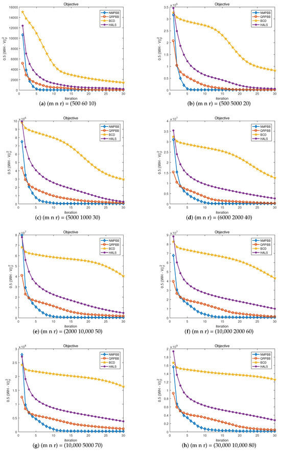
Figure 2. Objective value versus iteration on random problem ${min}_{W,H\ge 0}\frac{1}{2}{\parallel V-WH\parallel }_F^2$.

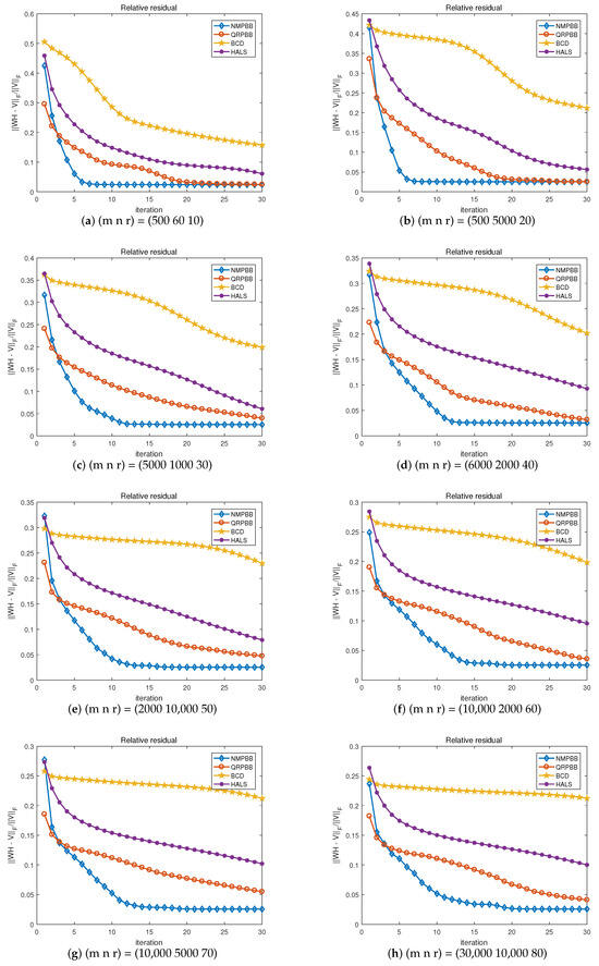
Figure 3. Residual value versus iteration on random problem ${min}_{W,H\ge 0}\frac{1}{2}{\parallel V-WH\parallel }_F^2$.

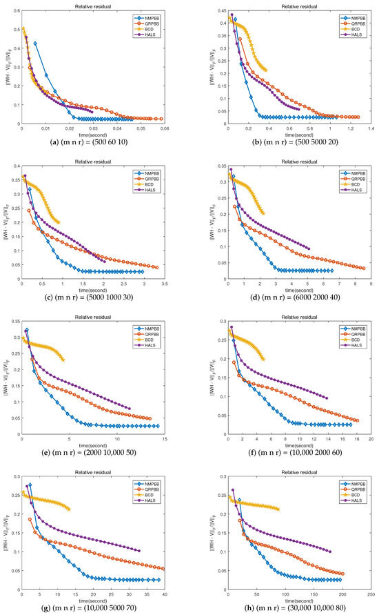
Figure 4. Residual value versus CPU time on random problem ${min}_{W,H\ge 0}\frac{1}{2}{\parallel V-WH\parallel }_F^2$.

4.3. Image Data

The ORL image database is a collection of 400 images of people’s faces belonging to 40 individuals representing 10 each. The dataset includes variations in lighting conditions, facial expressions (including whether they open their eyes, whether they smile), and facial details including whether they wear glasses. Some subjects have multiple photos taken at different times. The images were captured with the subject positioned upright and facing forward (allowing for slight movement to the sides). The background used was uniformly dark and even. All the images were taken against a dark homogeneous background with the subjects in an upright frontal position (with tolerance for some side movement). The pictures used are represented by the columns of the matrix V, and V has 400 rows and 1024 columns.

The Yale face database was created at the Yale Center for Computational Vision and Control. It consists of 165 gray-scale images, with each person in the database having 11 images associated with them. In total, there are 15 people. The facial images in question were captured under different lighting conditions (left-light, center-light, right-light), with various facial expressions (calm, cheerful, sorrowful, amazed, and blinking), and with or without glasses. The pictures used are represented by the rows of the matrix V, and V has 165 rows and 1024 columns.

For all the databases we used in (52), we performed a diverse casually generated starting iteration with $ϵ={10}^{-8}$, the maximum number of iterations (maxit) for all algorithms is set to 50,000, and the average results are presented in Table 2. From Table 2, we conclude that the QRPBB method converges in fewer iterations and CPU times than APBB2 and NeNMF, and in contrast to QRPBB, our NMPBB method requires 1/4 CPU time to satisfy the set tolerance. Although the residuals by NMPBB are not the smallest among all algorithms appearing for all the databases we use, the results of $pgn$ mean that solutions by NMPBB are nearer to the point of stationary.

Table 2. Experimental results on Yale and ORL datasets.

(m n r)	Alg	Iter	Niter	Pgn	Time	Residual
(165 1024 25)	NeNMF	3735.1	178,254.1	$4.41\times {10}^{-1}$	65.78	0.1930
	APBB2	3079.6	97,375.7	$6.42\times {10}^{-2}$	78.75	0.1930
	QRPBB	2711.1	54,215.7	$6.16\times {10}^{-2}$	42.25	0.1931
	NMPBB	1019.2	24,063.1	$2.60\times {10}^{-2}$	16.57	0.1930
(400 1024 25)	NeNMF	13,613.4	836,034.3	$7.71\times {10}^{-2}$	349.62	0.1117
	APBB2	9430.6	446,361.6	$6.88\times {10}^{-2}$	474.26	0.1117
	QRPBB	7593.5	213,178.5	$7.05\times {10}^{-2}$	205.26	0.1117
	NMPBB	1982.7	41,597.0	$6.25\times {10}^{-2}$	34.22	0.1117

4.4. The Importance of Relaxation Factor s

In the following content, the clear experimental results indicate that relaxation factor s is used for updating rules of $W_{t+1}$ and $H_{t+1}$. We implement NMPBB using diverse s given $s=0.1,0.3,0.7,1.0,1.3,1.7,1.9$ on synthetic datasets which are the same as those in Section 4.2. We set the required maximum number of iterations to 30, and the other parameters required in the experiment will have the same values as those in Section 4.2. Figure 5 shows the relationship between the relative residuals error and the run-time results. In Figure 5, we can see that the relaxation factor s fails to accelerate the convergence when $s<1$ and increasing constant s significantly accelerates the convergence when $1<s<2$. As for NMPBB, it seems that s = 1.7 is the best compared with other experimental values in terms of speed of convergence, and hence s = 1.7 was used as our NMPBB in all experiments.

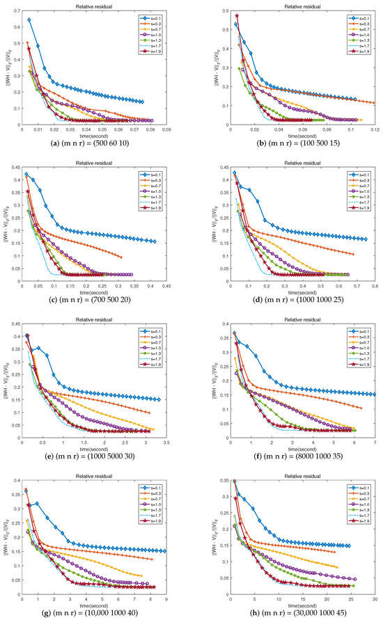
Figure 5. Residual value versus CPU time on random problem ${min}_{W,H\ge 0}\frac{1}{2}{\parallel V-WH\parallel }_F^2$.

5. Conclusions

In this paper, a prox-linear quadratic regularization objective function is presented, and the prox-linear term leads to strongly convex quadratic subproblems. Then, we propose a new line search technique based on the idea of [33]. According to the new line search, we put forward a global convergent method with larger step size to solve the subproblems. Finally, a series of numerical results are given to show that the method is a promising tool for NMF.

Symmetric nonnegative matrix factorization is a special but important class of NMF which has found numerous applications in data analysis such as various clustering tasks. Therefore, a direction for future research would be to extend the proposed algorithm to solve symmetric nonnegative matrix factorization problems.

References

- Gong, P.H.; Zhang, C.S. Efficient nonnegative matrix factorization via projected Newton method. Pattern Recognit. 2012, 45, 3557–3565. [Google Scholar] [CrossRef]
- Lee, D.D.; Seung, H.S. Learning the parts of objects by non-negative matrix factorization. Nature 1999, 401, 788–791. [Google Scholar] [CrossRef] [PubMed]
- Lee, D.D.; Seung, H.S. Algorithms for non-negative matrix factorization. Adv. Neural Process. Inf. Syst. 2001, 13, 556–562. [Google Scholar]
- Kim, D.; Sra, S.; Dhillon, I.S. Fast Newton-type methods for the least squares nonnegative matrix approximation problem. SIAM Int. Conf. Data Min. 2007, 1, 38–51. [Google Scholar]
- Paatero, P.; Tapper, U. Positive matrix factorization: A non-negative factor model with optimal utilization of error estimates of data values. Environmetrics 1994, 5, 111–126. [Google Scholar] [CrossRef]
- Ding, C.; Li, T.; Peng, W. On the equivalence between non-negative matrix factorization and probabilistic latent semantic indexing. Comput. Stat. Data Anal. 2008, 52, 3913–3927. [Google Scholar] [CrossRef]
- Chan, T.H.; Ma, W.K.; Chi, C.Y.; Wang, Y. A convex analysis framework for blind separation of nonnegative sources. IEEE Trans. Signal Process. 2008, 56, 5120–5134. [Google Scholar] [CrossRef]
- Ding, C.; He, X.; Simon, H. On the Equivalence of Nonnegative Matrix Factorization and Spectral Clustering. SIAM Int. Conf. Data Min. (SDM’05) 2005, 606–610. [Google Scholar]
- Févotte, C.; Bertin, N.; Durrieu, J.L. Nonnegative matrix factorization with the Itakura-Saito divergence: With application to music analysis. Neural Comput. 2009, 21, 793–830. [Google Scholar]
- Ma, W.K.; Bioucas-Dias, J.; Chan, T.H.; Gillis, N.; Gader, P.; Plaza, A.; Ambikapathi, A.; Chi, C.Y. A Signal Processing Perspective on Hyperspectral Unmixing. IEEE Signal Process. Mag. 2014, 31, 67–81. [Google Scholar] [CrossRef]
- Barzilai, J.; Borwein, J.M. Two-point step size gradient methods. IMA J. Numer. Anal. 1988, 8, 141–148. [Google Scholar] [CrossRef]
- Dai, Y.H.; Liao, L.Z. R-Linear convergence of the Barzilai-Borwein gradient method. IMA J. Numer. Anal. 2002, 22, 1–10. [Google Scholar] [CrossRef]
- Raydan, M. On the Barzilai-Borwein choice of steplength for the gradient method. IMA J. Numer. Anal. 1993, 13, 321–326. [Google Scholar] [CrossRef]
- Raydan, M. The Barzilai and Borwein gradient method for the large-scale unconstrained minimization problem. SIAM J. Optim. 1997, 7, 26–33. [Google Scholar] [CrossRef]
- Xiao, Y.H.; Hu, Q.J. Subspace Barzilai-Borwein gradient method for large-scale bound constrained optimization. Appl. Math. Optim. 2008, 58, 275–290. [Google Scholar] [CrossRef]
- Xiao, Y.H.; Hu, Q.J.; Wei, Z.X. Modified active set projected spectral gradient method for bound constrained optimization. Appl. Math. Model. 2011, 35, 3117–3127. [Google Scholar] [CrossRef]
- Han, L.X.; Neumann, M.; Prasad, U. Alternating projected Barzilai-Borwein methods for nonnegative matrix factorization. Electron. Trans. Numer. Anal. 2009, 36, 54–82. [Google Scholar]
- Huang, Y.K.; Liu, H.W.; Zhou, S.S. Quadratic regularization projected alternating Barzilai-Borwein method for nonnegative matrix factorization. Data Min. Knowl. Discov. 2015, 29, 1665–1684. [Google Scholar] [CrossRef]
- Huang, Y.K.; Liu, H.W.; Zhou, S.S. An efficint monotone projected Barzilai-Borwein method for nonnegative matrix factorization. Appl. Math. Lett. 2015, 45, 12–17. [Google Scholar] [CrossRef]
- Li, X.L.; Liu, H.W.; Zheng, X.Y. Non-monotone projection gradient method for non-negative matrix factorization. Comput. Optim. Appl. 2012, 51, 1163–1171. [Google Scholar] [CrossRef]
- Liu, H.W.; Li, X. Modified subspace Barzilai-Borwein gradient method for non-negative matrix factorization. Comput. Optim. Appl. 2013, 55, 173–196. [Google Scholar] [CrossRef]
- Bonettini, S. Inexact block coordinate descent methods with application to non-negative matrix factorization. IMA J. Numer. Anal. 2011, 31, 1431–1452. [Google Scholar] [CrossRef]
- Zdunek, R.; Cichocki, A. Fast nonnegative matrix factorization algorithms using projected gradient approaches for large-scale problems. Comput. Intell. Neurosci. 2008, 2008, 939567. [Google Scholar] [CrossRef]
- Bai, J.C.; Bian, F.M.; Chang, X.K.; Du, L. Accelerated stochastic Peaceman-Rachford method for empirical risk minimization. J. Oper. Res. Soc. China 2023, 11, 783–807. [Google Scholar] [CrossRef]
- Bai, J.C.; Han, D.R.; Sun, H.; Zhang, H.C. Convergence on a symmetric accelerated stochastic ADMM with larger stepsizes. CSIAM Trans. Appl. Math. 2022, 3, 448–479. [Google Scholar]
- Bai, J.C.; Hager, W.W.; Zhang, H.C. An inexact accelerated stochastic ADMM for separable convex optimization. Comput. Optim. Appl. 2022, 81, 479–518. [Google Scholar] [CrossRef]
- Bai, J.C.; Li, J.C.; Xu, F.M.; Zhang, H.C. Generalized symmetric ADMM for separable convex optimization. Comput. Optim. Appl. 2018, 70, 129–170. [Google Scholar] [CrossRef]
- Bai, J.C.; Zhang, H.C.; Li, J.C. A parameterized proximal point algorithm for separable convex optimization. Optim. Lett. 2018, 12, 1589–1608. [Google Scholar] [CrossRef]
- Guan, N.Y.; Tao, D.C.; Luo, Z.G.; Yuan, B. NeNMF: An optimal gradient method for nonnegative matrix factorization. IEEE Trans. Signal Process. 2012, 60, 2882–2898. [Google Scholar] [CrossRef]
- Xu, Y.Y.; Yin, W.T. A globally convergent algorithm for nonconvex optimization based on block coordinate update. J. Sci. Comput. 2017, 72, 700–734. [Google Scholar] [CrossRef]
- Zhang, H.C.; Hager, W.W. A nonmonotone line search technique and its application to unconstrained optimization. SIAM J. Optim. 2004, 14, 1043–1056. [Google Scholar] [CrossRef]
- Dai, Y.H. On the nonmonotone line search. J. Optim. Theory Appl. 2002, 112, 315–330. [Google Scholar] [CrossRef]
- Gu, N.Z.; Mo, J.T. Incorporating nonmonotone strategies into the trust region method for unconstrained optimization. Comput. Math. Appl. 2008, 55, 2158–2172. [Google Scholar] [CrossRef]
- Ahookhosh, M.; Amini, K.; Bahrami, S. A class of nonmonotone Armijo-type line search method for unconstrained optimization. Optimization 2012, 61, 387–404. [Google Scholar] [CrossRef]
- Nosratipour, H.; Borzabadi, A.H.; Fard, O.S. On the nonmonotonicity degree of nonmonotone line searches. Calcolo 2017, 54, 1217–1242. [Google Scholar] [CrossRef]
- Glowinski, R. Numerical Methods for Nonlinear Variational Problems; Springer: New York, NY, USA, 1984. [Google Scholar]
- Birgin, E.G.; Martinez, J.M.; Raydan, M. Nonmonotone spectral projected gradient methods on convex sets. SIAM J. Optim. 2000, 10, 1196–1211. [Google Scholar] [CrossRef]
- Cichocki, A.; Zdunek, R.; Amari, S.I. Hierarchical ALS Algorithms for Nonnegative Matrix and 3D Tensor Factorization. Lect. Notes Comput. Sci. Springer 2007, 4666, 169–176. [Google Scholar]
- Xu, Y.Y.; Yin, W.T. A block coordinate descent method for regularized multi-convex optimization with applications to nonnegative tensor factorization and completion. SIAM J. Imaging Sci. 2015, 6, 1758–1789. [Google Scholar] [CrossRef]
- Lin, C.J. Projected Gradient Methods for non-negative matrix factorization. Neural Comput. 2007, 19, 2756–2779. [Google Scholar] [CrossRef] [PubMed]
- Gillis, N. The why and how of nonnegative matrix factorization. arXiv 2015, arXiv:1401.5226v2. [Google Scholar]
Disclaimer/Publisher’s Note: The statements, opinions and data contained in all publications are solely those of the individual author(s) and contributor(s) and not of MDPI and/or the editor(s). MDPI and/or the editor(s) disclaim responsibility for any injury to people or property resulting from any ideas, methods, instructions or products referred to in the content. |
© 2024 by the authors. Licensee MDPI, Basel, Switzerland. This article is an open access article distributed under the terms and conditions of the Creative Commons Attribution (CC BY) license (https://creativecommons.org/licenses/by/4.0/).