Improving the Efficiency of Software Reliability Demonstration Testing by Introducing Testing Effectiveness

Abstract

For highly reliable software systems, it is expensive, time consuming, or even infeasible to perform reliability testing via a conventional software reliability demonstration testing (SRDT) plan. Moreover, in the traditional SRDT approach, the various characteristics of the software system or test sets are not considered when making the testing schemes. Some studies have focused on the effect of software testability on SRDT, but only limited situations were discussed, and many theoretical and practical problems have been left unresolved. In this paper, an extended study on the quantitative relation between test effectiveness (TE) and test effort for SRDT is proposed. Theoretical derivation is put forward by performing statistical analysis for the test suite according to TE. The combinations of all the cases of zero-failure and revealed nonzero failure, as well as discrete-type software and continuous-type software, are studied with the corresponding failure probability models constructed. That is, zero-failure and nonzero failure, as well as discrete-type software and continuous-type software, respectively, constitute the symmetry and asymmetry of SRDT. Finally, we illustrated all the models and performed applications on the Siemens program suite. The experimental results show that within the same limitation of requirements and confidence levels, this approach can effectively reduce the number of test cases and the test duration, i.e., accelerate the test process and improve the efficiency of the SRDT.

1. Introduction

With the development of network and computing technology, more and more software applications are being applied to various fields of society, such as systems-of-systems (SoSs), cyber–physical systems (CPSs), and distributed systems [1]. With the increasing demand for software system reliability, reliability demonstration testing serves as a solution for validation and acceptance testing [2]. That is, SRDT is an important representative testing method for evaluating whether a software system has achieved a certain level of reliability at a given level of confidence, and for helping people make decisions on delivery or acceptance [3,4]. The relevant methods can be divided into two categories; one is fixed-duration testing methods, such as Laplace’s rule of succession [5], TRW [6], Bayesian [7], life testing [8] and Bayesian zero-failure (BAZE) testing [9,10]. Another is non-fixed-duration testing methods, such as probability ratio sequential testing (PRST) [11] and the t-distribution method [12]. In this paper, the research is only conducted in the context of the fixed-duration SRDT method.

However, traditional SRDT based on the number of failures depends on the testing of large samples, which is not feasible for highly reliable software systems [13,14]. How to reduce the sample size is currently a challenge that needs to be solved in the field of SRDT. Most existing SRDT methods assume that the same number of statistical test cases is needed for different software systems to reach the same expected reliability level under the same confidence limit [15], i.e., statistical test sets with the same number of test cases have the same statistical power, and do not consider the effect induced by the characteristics of the software system itself. This may be somewhat counterintuitive, as we often assume that high-quality software may require fewer test cases. In contrast, many researchers have introduced software products or process measurements into reliability evaluation, e.g., code coverage [16,17], which has improved the accuracy of evaluation models.

Moreover, since the 1990s, software testability has received much more attention in software engineering [18,19,20] and has been introduced into software reliability evaluation. Software testability is regarded as the ability or degree to which a software supports testing in a given test context, which is always represented by the probability of the fault detection rate [21,22,23]. Since testability could affect test implementation efficiency, it could also affect reliability testing. Chen et al. [24] has demonstrated that testability affects the number of test cases needed to achieve a given reliability level; that is, if a software has better testability, fewer test cases will be needed for certain reliability assurance targets.

Based on the concept of software testability, Kuball et al. suggested as a concept to extract a test set’s different properties, which are brought into quantitative reliability assessment to base a reliability estimate on those properties. For example, they propose a model to combine the fault detection power of a given test set with the statistical power of the test set, i.e., they want to employ as much information as possible on the software product, test set, and operational environment. They propose a method that can be used to analyze the influence on a reliability measure of any given test set, and also point that further considerations are deserved on how their concepts could be exploited when the number of statistical test cases required to obtain a specified reliability target is very large [25]. They conducted such research because they had previously completed a relatively complex statistical testing task. Not only did they summarize the difficulty and key techniques of statistical testing but this also prompted them to think about another question: whether they could discover as many different characteristics of the test set as possible [26,27,28]. Kuball et al. demonstrate the effectiveness of statistical testing in terms of error detection when compared to other testing techniques, employed using the example of a Programmable Logic System (PLS) [26]. They explore the applicability of statistical (software) testing (ST) to the example of a real safety-related software application and discuss the key points arising in this task, highlighting the unique and important role ST can play within the wider task of software verification [27]. They also present an experience report that describes the successful application of statistical software testing to a large-scale real-world equipment replacement project. A total of 395 statistical tests with no failure were achieved, providing at least 98% confidence that the safety claim was met [28].

In our previous work [29], we found Kuball et al. provided an interesting idea in [25], so we attempted to introduce their concept into our SRDT plan to reduce the minimum sample size. By comparing the number of SRDT sets considering TE with that of traditional approaches without considering TE, we proved that conventional statistical methods and Bayesian priori statistical methods are conservative estimation methods, assuming that TE is equal to zero [29]. To the best of our knowledge, we were the first to explicitly introduce testability as a factor into the quantitative expression of the SRDT plan.

However, in [29], we only give the mathematical expression for a zero-failure SRDT plan, and we do not give an expression considering a nonzero failure SRDT plan, e.g., r = 1,2,… The reason is that [25] only gives input space models with zero or nonzero cases; they do not give an input space model at r = 1,2,… Based on the above ideas, this paper attempts to construct an input space model of r = 1,2,…, and then explicitly introduces the expression of TE into the SRDT mathematical expression with r = 1,2,… Although there are many ways to accelerate software reliability testing, to the best of our knowledge, we are the first to conduct such research. Due to space limitations, you can refer to the review on the SRDT method in [30] to reach such conclusions. To address the aforementioned issues, we have made several contributions to our work, including the following:

• We propose the principle of introducing TE into SRDT under zero and nonzero fault conditions, and provide mathematical derivations of the models for both scenarios.
• We provide an improved SRDT framework integrated with a uniform measurement of TE, which takes into account both discrete-type and continuous-type software, both with zero-failure situations and failure-revealed situations.
• We give the estimation method of TE based on the statistical fault injection, which considers the statistical characteristics of the software reliability test case set.
• We conduct a numerical case study on the Siemens program suite to demonstrate the practical application and effectiveness of our proposed method. In total, seven programs are taken into consideration and the experimental results provide evidence for its potential to improve software demonstration testing efficiency.

The remainder of this paper is structured as follows. In Section 2, we outline the background and related works in the field of SRDT. In Section 3, we describe the principle of the SRDT approach, introducing TE in the cases of zero-failure and revealed failures, respectively, and present the estimation method of TE based on the statistical fault injection method, together with the improved SRDT framework. In Section 4, we demonstrate the practical application of our method through a numerical case study of the Siemens program suite. Finally, in Section 5, we outline our conclusions and identify potential future research directions.

2. Related Works

The aim of our work is to propose an approach to improve the efficiency of SRDT by introducing TE. Thus, we review related works in the literature that address (i) SRDT and the software reliability acceleration testing method, (ii) software testability and TE, and (iii) software fault injection.

2.1. SRDT and Software Reliability Acceleration Testing Method

i.

SRDT Method

US MIL-HDBK-781A specifies two reliability demonstration testing methods for the hardware products as standard procedures: PRST and fixed-duration testing (FDT) [11]. It is then recommended that reliability demonstration testing be applied to software systems as well to certify that the required level of reliability has been achieved [4]. SRDT is based on two risks, that is, prespecified producer and consumer risks, and this process determines the maximum number of software failures during testing. As an alternative, Tal et al. proposed single-risk sequential testing (SRST) based on PRST [13,31], which satisfies the consumer risk criterion, while PRST provides much less consumer risk than required.

From a Bayesian point of view, Martz and Waller proposed a zero-failure reliability demonstration testing method named Bayesian zero-failure (BAZE) reliability demonstration testing [30,32,33]. Then, the concept of zero-failure reliability demonstration testing was introduced into software products [4].

For software such as those used to control production lines and computer operating systems, where reliability is discussed in terms of mean time between software failures (MTBF) and the number of bugs remaining in the software, Sandoh [4,33] proposed a continuous model for SRDT. Cho [32] and Sandoh [30] then investigated a discrete model. But none of the models mentioned above had taken into account the damage size of software failures. As such, Sandoh [33] proposed a continuous model for SRDT that considers the damage size of software failures as well as the number of software failures in the test.

Thus, the relevant methods can be divided into two categories; one is fixed-duration testing methods, and the other is non-fixed-duration testing methods. In this paper, the research is only conducted in the context of fixed-duration SRDT.

ii.

Software Reliability Acceleration Testing Method

Though SRDT is recognized as an important means, its large number of test cases often become a bottleneck for its large-scale promotion and application in practice. Therefore, more and more researchers have carried out research on whether it is possible to accelerate the process of software reliability testing under the premise of maintaining its essential characteristics.

Chan et al. gave the definition of software accelerated stress testing, and explained the basic principles of accelerated testing in combination with hardware [34]. Based on the idea of importance sampling, Tang [35] and Hecht [36] proposed to increase the sampling of key or critical operations to accelerate the exposure of defects that affect system safety. The inclusion of coverage information is also one of the ideas of software reliability acceleration testing, and Chen [37] and Bishop [38] proposed a method to predict software failures using information such as decision coverage and dataflow coverage. The method uses “parameterization factors” to eliminate the execution time that neither increases coverage nor causes software failure during the testing process so as to solve the problem of the “saturation effect” of the testing method.

From the abovementioned studies, it can be seen that the traditional SRDT method is mainly based on the idea of statistics or Bayesian theory, and proposes a general SRDT scheme that is only for discrete-type software and continuous-type software. The existing software reliability testing acceleration methods are based on importance sampling, the introduction of coverage information, parameterization factors, and consideration of a saturation effect, but none of them consider the software quality attribute in the acceleration process, that is, software with different testabilities may require a different number of SRDT cases, which can be analyzed for a specific software, rather than treating all software as the same.

2.2. Software Testability and TE

i.

Definitions of Software Testability

Software testability is an important quality attribute that is of great significance for improving software design and testing efficiency and fundamentally improving software quality.

IEEE Software Engineering Standard Terminology and the ISO Quality Model give definitions of software testability as follows. Definition 1: whether a software system or component is easy to test and the performance of a software system or component that allows it to be adequately tested in accordance with the test criterion [21]. Definition 2: software attributes that need to be verified to confirm the correctness of the modified software system [39]. These two definitions are too abstract and lack operability. Therefore, the following definitions are given. Definition 3: the probability that a program will fail in a random black-box test when there is a defect in the program [40]. Definition 4: the ease with which software can be tested in a given test context [41]. Definition 5: the minimum number of test cases required to meet the adequacy requirements required by the testing criteria when testing software against these criteria [42].

The main differences between these definitions are as follows: first, whether testability is considered an internal or external quality property of the software; second, whether testability is measured by the probability of finding a defect in the test or the number of test cases in which the software meets the adequacy requirements of a given test criterion.

ii.

Metrics for Software Testability

Freedman proposed that the main factor affecting testability is the inconsistency of input and output, which is defined as the observability and controllability of the software, respectively. Testability was defined as the extension required to transform a piece of software to be observable and controllable, represented by a binary group [43].

Voas et al. believed that the main factor affecting testability is that some data information during software execution is not visible at the output end of the software, that is, the loss of information, including implicit information loss and explicit information loss. The implicit loss of information (two or more different input data producing the same output) makes it impossible to judge the corresponding input based on the output of the software. The ratio of the potential of the function definition domain to the output domain, known as the domain–range ratio (DRR), can roughly reflect the probability of implicit information loss. As the DRR increases, the potential for information loss increases, and the testability of the software declines [40].

McGregor et al. utilized the ratio between the output size of the method and the size of all potentially accepted inputs as a testability metric. The minimum testability measure for all methods in a class is used as a testability measure for that class [44]. Gao divided software testability into five sub-attributes: comprehensibility, test supportability, traceability, controllability, and observability. The area enclosed by the results of these five sub-attributes is used as a software testability measure [42].

Richard built a metric model based on the decomposition of the program control flow diagram. First, the number of test cases required for each subgraph is defined, and then the number of test cases required for the whole program to meet the coverage criterion is calculated according to the sequential structure, loop structure, and selection structure of the program, which is used as a testability measure of the whole software [45].

Nguyen et al. synthesized Freedman’s ideas of controllability and observability of programs or modules and dataflow analysis methods, and used information theory analysis methods and the analysis results of the dataflow in a program to determine the relationship between the input and output of each module in the program’s execution, as well as the output/input range of the program module itself, as a measure of controllability and observability [46].

Bruce used the hierarchy of inheritance trees and the coupling relationship between classes as a measure of testability for object-oriented (OO) programs [47]. Jungmayr measured testability by dependencies between classes [41]. Sohn utilized information entropy and fault tree analysis to calculate the testability of software or modules [48]. Khoshgftaar used neural networks to predict testability [49]. Bruntink predicted testability by analyzing the correlation between the source code and the test code for OO programs [50].

The defect/failure model reflects the dynamic behavior of the software during testing [51]. According to this model, a test that can find a defect should meet three basic conditions [51], that is, when the test executes a piece of code containing a defect, it will affect the state of the program, and the faulty state will be transmitted to the output.

Voas proposed a propagation–infection–execution (PIE) approach to measure testability. The shortcoming of the PIE method is that it is too complex. In order to take advantage of the PIE method while reducing its complexity, Jin et al. improved the PIE method based on software code structure, semantics, and input distribution assumptions [52]. Bruce estimated testability by sampling test data to calculate the probability of code execution, infection, and propagation of a statement in the test set [47].

iii.

Metrics for software TE

To measure the effectiveness of the test criterion is an important problem for software quality assurance. The test criterion defines the basic principle for the selection or generation of test cases, and specifies the basic requirement that the test set needs to meet when the software is adequately tested. However, there is currently no consistent way to represent the effectiveness of the test criterion. From a statistical point of view, any TE of a test set that satisfies a certain test criterion has some stability. However, for a single test set, the specific test cases contained in it depend on the experience and skill of the tester, and the test case generation has a large randomness, resulting in a certain randomness in the TE. There are two main ways to measure TE: the probability that at least one defect will be found by the test (P-measure) or the expected value by which the test will be able to find the defect (E-measure).

Frankl investigated the effectiveness of branch testing and dataflow testing at different coverage levels [53]. Hutchins argued that when the coverage level is less than 100%, there is the same level of coverage, but it covers different parts of the software, resulting in a change in the effectiveness measure, which may affect the analysis of the effectiveness of the criterion [54]. Moreover, the ability of a test to detect defects can only be maximized when the adequacy of the test reaches 100% of the criterion [55]. Kuball used the defect detection capability of the test set to represent TE [25]. From the abovementioned studies, it can be seen that there are certain conflicting research results in the field of software testability, e.g., a variety of definitions and measurement methods are given, and some definitions and measurement methods have been recognized by the industry.

2.3. Software Fault Injection

Software fault injection is currently an effective method to evaluate the reliability mechanism in a system [56]. The fault injection technology accelerates the failure process of the target system by injecting multiple faults into the target system, and then obtains the operating state of the system when the fault occurs by monitoring the system after the injection of faults, and then compares it with the normal operation state of the system so as to evaluate the correctness and effectiveness of the fault tolerance mechanism of the target system.

There are many ways to inject faults, such as destroying programs or data in memory; dynamically modifying code and data; changing the execution process and control flow and replacing code; reassembling code using traps; injecting faults with debug registers; and so on.

Fault injection can be used for fault detection, failure prediction, and acceptance testing. Program mutation is the main method of static fault injection in software, which is mainly used to evaluate the adequacy of the test set and the prediction of latent faults in the software [57,58,59]. For statistical fault injection, faults are randomly injected into the program according to the probability distribution, and then statistical tests are performed. As a result, this allows for a better simulation of the true distribution of software failures and statistical estimates. Kuball et al. used program mutation to obtain the fault detection capability of the test by statistical fault injection [25]. Leveugle et al. proposed to use the failure occurrence probability and fault interval [60,61] to statistically determine the number of faults injected.

From the abovementioned studies, it can be seen that there are certain research results in the field of software fault injection, and a variety of fault injection methods are given. Due to the particularity of the testability of software reliability test cases, it is necessary to use statistical fault injection instead of fault injection in general software testing.

In summary, dissimilar to the existing works, this paper presents the following:

• TE is introduced into the SRDT method as an acceleration factor.
• For discrete-type software and continuous-type software, corresponding demonstration test plans are established for cases of zero-failure and revealed nonzero failure.
• Based on the statistical fault injection method, a quantitative estimation approach of software TE for SRDT is considered.

3. Proposed Method

This paper is mainly divided into three parts as follows: the modeling of introducing TE into SRDT, taking into account both zero and nonzero failure conditions, the estimation method of TE, and the SRDT framework integrated with TE. Figure 1 illustrates the research framework of this paper. From this section onward, the improved SRDT method will be studied according to the research ideas shown in this framework.

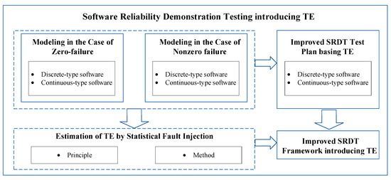
Figure 1. Research framework.

3.1. TE-Introduced SRDT in the Case of Zero-Failure (TE-SRDT-0F)

3.1.1. Conventional SRDT Process

The conventional SRDT procedure is shown in Figure 2.

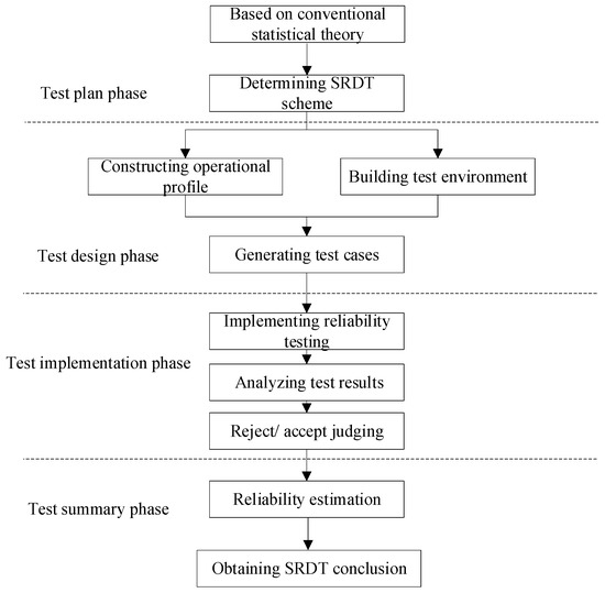
Figure 2. Conventional SRDT procedure.

From Figure 2, we note that the key step in SRDT is determining the statistical scheme for a given demand, i.e., an upper confidence limit and the expected value for reliability. Therefore, first, we introduce the principle of SRDT integrated with TE and then describe how to determine the statistical scheme and how to estimate TE. It should be noted that in this paper, we aim to provide an improved SRDT scheme by introducing TE, so our research is only focused on the “Test plan phase”, as shown in Figure 2.

3.1.2. SRDT Introducing TE in the Case of Zero-Failure

a.

The Basic Principle in the Case of Zero-failure

Let $P$ denote a program, $T$ denote a test set, and ${\phi }_T$ denote TE [25,29]. ${\phi }_T=P_r(T det\begin{array}{cccc}ects& fact& that& P\end{array}\begin{array}{cc}is& faulty)\end{array}$, where ${\phi }_T$ represents the probability of the test set, revealing failures in the execution of $P$ if there are faults left in $P$, and $P_r(.)$ represents the probability of a random event. Suppose $N$ test cases are implemented and no failures are found, i.e., the failure number $r=0$, and the test time is $T_a$. We use $\Re$ to represent the result, so $\Re$ = {the number of test cases is $N$, the number of failures is 0, and the total test duration is $T_a$}. $\Omega$ is defined as the program space, consisting of all possible programs $P^{\prime }$, and $P^{\prime }$ is any mutation version derived from $P$. Suppose $P^G$ is a faultless version of the program, i.e., a mutation version with a zero fault derived from $P$; obviously, $P^G$ is also in $\Omega$. Then, we divide $\Omega$ into two subsets, $A_0$ and $A_1$, as shown in Figure 3. $A_0$ is the set of programs $P^{\prime }$ with the following property: $P^{\prime }$ contains faults, which cannot be revealed by executing $T$, so $A_0=\left\{P^{\prime }|\forall P^{\prime }\in \Omega ,\forall fault\in P^{\prime },\begin{array}{cccc}0& failures& by& T\end{array}\right\}$, where $fault\in P^{\prime }$ means faults contained in program $P^{\prime }$, and 0 failures by $T$ means test set $T$ cannot reveal failures. $A_1$ is the set of programs $P^{\prime }$ with either of the following properties: $P^{\prime }$ contains faults, test set $T$ can reveal at least 1 failure, or $P^{\prime }$ is correct. It is denoted as $A_1=\left\{P^{\prime }|\forall P^{\prime }\in \Omega ,\forall fault\in P^{\prime },1failure\begin{array}{cc}at& least\end{array}\right\}\cup P^G$. Therefore, we have

$$P_r(P\in A_1|{\phi }_T,\Re )={\phi }_T$$

(1)

$$P_r(P\in A_0|{\phi }_T,\Re )=1-{\phi }_T$$

(2)

where $P_r(P\in A_i|{\phi }_T,\Re )$, and $(i=0,1)$ indicates the probability that $P$ belongs to $A_i$. $P_r(P\in A_0|{\phi }_T,\Re )$ indicates the probability that $P$ contains faults but cannot be revealed by executing $T$, and $P_r(P\in A_1|{\phi }_T,\Re )$ indicates the probability that $P$ contains faults and can be revealed by executing $T$.

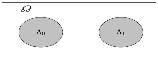
Figure 3. The division of program space $\Omega$ in the case of zero-failure [29].

We note that $\Re$ can occur under the following conditions: (1) $P\in A_0$, for which the failure rate or failure probability distribution is unknown; (2) $P\in A_1$, and $P=P^G$. Let $A_r(r=0,1)$ denote the events $“P\in A_0”,“P\in A_1”$, and let $f(\theta |\Re ,{\phi }_T)$ indicate the conditional probability density function of the failure rate for continuous-type software or failure probability for discrete-type software given the observation of $\Re$ and the probability ${\phi }_T$. Then, we have

$$f(\theta |\Re ,{\phi }_T)=f(\theta ,A_0|\Re ,{\phi }_T)+f(\theta ,A_1|\Re ,{\phi }_T)$$

(3)

The first term on the right side of (3) is

$$\begin{array}{ll}f(\theta ,A_0& |\Re ,{\phi }_T)={\displaystyle \frac{f(\theta ,A_0,\Re ,{\phi }_T)}{\mathrm{Pr}(\Re ,{\phi }_T)}}={\displaystyle \frac{f(\theta |A_0,\Re ,{\phi }_T)\mathrm{Pr}(A_0|\Re ,{\phi }_T)\mathrm{Pr}(\Re ,{\phi }_T)}{\mathrm{Pr}(\Re ,{\phi }_T)}}\\ & =f(\theta |A_0,\Re ,{\phi }_T)\mathrm{Pr}(A_0|\Re ,{\phi }_T)=f(\theta |A_0,\Re ,{\phi }_T)(1-{\phi }_T)\end{array}$$

(4)

The second term on the right side of (3) is

$$\begin{array}{ll}f(\theta ,A_1& |\Re ,{\phi }_T)={\displaystyle \frac{f(\theta ,A_1,\Re ,{\phi }_T)}{\mathrm{Pr}(\Re ,{\phi }_T)}}={\displaystyle \frac{f(\theta |A_1,\Re ,{\phi }_T)\mathrm{Pr}(A_1|\Re ,{\phi }_T)\mathrm{Pr}(\Re ,{\phi }_T)}{\mathrm{Pr}(\Re ,{\phi }_T)}}\\ & =f(\theta |A_1,\Re ,{\phi }_T)\mathrm{Pr}(A_1|\Re ,{\phi }_T)=f(\theta |A_1,\Re ,{\phi }_T){\phi }_T\end{array}$$

(5)

Substituting (4) and (5) into (3), we have

$$f(\theta |\Re ,{\phi }_T)=f(\theta |A_0,\Re ,{\phi }_T)(1-{\phi }_T)+f(\theta |A_1,\Re ,{\phi }_T){\phi }_T$$

(6)

where $f(\theta |A_0,\Re ,{\phi }_T)$ is the conditional probability density function of the failure rate or failure probability when event $“P\in A_0”$ occurs. Thus, given the observation of $\Re$, i.e., $r=0$, the probability density function of the failure rate or failure probability is expressed by a Bayesian posterior distribution with no a priori information $f(\theta |A_0,\Re ,{\phi }_T)$.

For continuous-type software, we have [7,30]

$$f(\theta |A_0,\Re ,{\phi }_T)=Gamma(1,T_a)(\theta )$$

(7)

For discrete-type software, we have [7,30]

$$f(\theta |A_0,\Re ,{\phi }_T)=\beta (1,N+1)(\theta )$$

(8)

For $f(\theta |A_1,\Re ,{\phi }_T)$, $P=P^G$, which means that the software contains no faults and the failure rate or failure probability is 0, i.e., the probability of event $\theta =0$ is 1. We use the $delta$-distribution to approximately express the distribution of the failure rate or failure probability [25]:

$$\delta (\theta )=\{\begin{array}{cc}1/\epsilon & \theta \in [0,\epsilon ],\epsilon >0,\epsilon \to 0\\ 0& \theta \notin [0,\epsilon ]\end{array}$$

(9)

Therefore, for continuous-type software, the failure rate density function introducing TE in the case of zero-failure is

$$f(\theta |\Re ,{\phi }_T)=Gamma(1,T_a)(\theta )\cdot (1-{\phi }_T)+\delta (\theta )\cdot {\phi }_T$$

(10)

For discrete-type software, the failure probability density function introducing TE in the case of zero-failure is

$$f(\theta |\Re ,{\phi }_T)=\beta (1,N+1)(\theta )\cdot (1-{\phi }_T)+\delta (\theta )\cdot {\phi }_T$$

(11)

Given the reliability demand of SRDT $({\theta }_0,C)$, where ${\theta }_0$ is the expected failure rate or failure probability and $C$ is the upper confidence limit, from (6), the following can be derived to obtain the TE-SRDT-0F scheme:

$$P_r(\theta \le {\theta }_0)={\displaystyle {\int }_0^{{\theta }_0}f(\theta |\Re ,{\phi }_T)}d\theta ={\displaystyle {\int }_0^{{\theta }_0}f(\theta |A_0,\Re ,{\phi }_T)\cdot (1-{\phi }_T)+}f(\theta |A_1,\Re ,{\phi }_T)\cdot {\phi }_{T}d\theta \ge C$$

(12)

b.

Using TE-SRDT-0F to Make a Test Plan

(1)

Test Plan with TE-SRDT-0F for Continuous-type Software (TE-SRDT-0F-CS)

Let $\lambda$ indicate the failure rate for continuous-type software. In the case of zero-failure, the probability density function of the failure rate $\lambda$ with respect to the introduced TE is $f(\lambda |\Re ,{\phi }_T)=Gamma(1,t)(\lambda )\cdot (1-{\phi }_T)+\delta (\lambda )\cdot {\phi }_T$. For the given demand $({\lambda }_0,C)$ (where ${\lambda }_0$ is the expected failure rate and $C$ is the upper confidence limit), we can obtain the minimum test time $T_a$ for TE-SRDT-0F-CS from (12), which is the minimum value of $t$ in the following formula:

$$\begin{array}{c}\mathrm{Pr}(\lambda \le {\lambda }_0)={\displaystyle {\int }_0^{{\lambda }_0}f(\lambda |\Re ,{\phi }_T})d\lambda ={\displaystyle {\int }_0^{{\lambda }_0}Gamma(1,t)(\lambda )\cdot (1-{\phi }_T)}d\lambda +{\displaystyle {\int }_0^{{\lambda }_0}\delta (\lambda )\cdot {\phi }_T}d\lambda \\ =(1-{\phi }_T)\cdot {\displaystyle {\int }_0^{{\lambda }_0}Gamma(1,t)(\lambda )}d\lambda +{\phi }_T=(1-{\phi }_T)\cdot (1-e^{-t{\lambda }_0})+{\phi }_T\ge C\end{array}$$

(13)

Therefore, we have

$$t\ge -{\displaystyle \frac{1}{{\lambda }_0}}\ln \left({\displaystyle \frac{1-C}{1-{\phi }_T}}\right)$$

(14)

From (14), the minimum test time $T_a$ is

$$T_a=-{\displaystyle \frac{1}{{\lambda }_0}}\ln \left({\displaystyle \frac{1-C}{1-{\phi }_T}}\right)$$

(15)

When TE is not considered, for continuous-type software in the case of zero-failure, the probability density function of failure rate $\lambda$ is $f(\lambda )=Gamma(1,t)(\lambda )$. For the given demand $({\lambda }_0,C)$, the demanded $T_a$ is the minimum value of $t$ in (16).

$$\mathrm{Pr}(\lambda \le {\lambda }_0)={\displaystyle {\int }_0^{{\lambda }_0}f(\lambda })d\lambda ={\displaystyle {\int }_0^{{\lambda }_0}Gamma(1,t)(\lambda )}d\lambda =1-e^{-t{\lambda }_0}\ge C$$

(16)

which means that $T_a$ is

$$T_a=-{\displaystyle \frac{1}{{\lambda }_0}}\ln \left(1-C\right)$$

(17)

From (15) and (17), we note that the SRDT without considering the TE is a special case in which ${\phi }_T$ is 0. For (15), suppose ${\phi }_T$ is an independent variable and $T_a$ is a dependent variable, which means that $T_a$ is a function of ${\phi }_T$. To compute the derivation of ${\phi }_T$, we have

$$T_a^{\prime }=-{\displaystyle \frac{1}{{\lambda }_0}}\cdot {\displaystyle \frac{1-{\phi }_T}{1-C}}\cdot {\displaystyle \frac{1-C}{{(1-{\phi }_T)}^2}}=-{\displaystyle \frac{1}{{\lambda }_0(1-{\phi }_T)}}$$

(18)

because ${\lambda }_0>0$, $0\le {\phi }_T<1$, ${T^{\prime }}_a<0$. This means that $T_a$ is a decreasing function of ${\phi }_T$. $T_a$ decreases as ${\phi }_T$ increases. When ${\phi }_T=0$, $T_a$ reaches the maximum value of $-{\displaystyle \frac{1}{{\lambda }_0}}\ln (1-C)$. Therefore, the demanded SRDT time with introduced TE is shorter than that without considering TE. Table 1 shows the relationship between the SRDT time and the reliability demand in the case of zero-failure and when TE is introduced.

Table 1. The relationship between test time $T_a$ and $({\lambda }_0,C,{\phi }_T)$ in the case of zero-failure.

${\mathit{\lambda }}_{\mathbf{0}}$	${\mathit{\phi }}_{\mathit{T}}$	${\mathit{T}}_{\mathit{a}}$
		$\mathit{C}=0.9$	$\mathit{C}=0.95$	$\mathit{C}=0.99$
0.01	0	230.26	299.58	460.52
	0.5	160.94	230.26	391.21
	0.9	--	69.32	230.26
0.001	0	2302.59	2995.74	4605.18
	0.5	1609.44	2302.59	3912.03
	0.9	--	693.15	2302.59
0.0001	0	23,025.86	29,957.33	46,051.71
	0.5	16,094.38	23,025.86	39,120.24
	0.9	--	6931.48	23,025.86
0.00001	0	230,258.51	299,573.23	460,517.02
	0.5	160,943.79	230,258.51	391,202.30
	0.9	--	69,314.72	230,258.51

Obviously, the conventional test plan without introducing TE is a special case in which ${\phi }_T=0$. Taking ${\lambda }_0=0.001$$C=0.99$ as an example, the test time in the conventional scheme is 4605; for the TE-introduced scheme, suppose ${\phi }_T=0.5$, and the test time is 3912, which is a 15.1% reduction. Supposing ${\phi }_T=0.9$, the test time is 2302, which is a 50% reduction.

(2)

Test Plan with TE-SRDT-0F for Discrete-type Software (TE-SRDT-0F-DS)

Let $\lambda$ indicate the failure rate for continuous-type software. In the case of zero-failure, the probability density function of the failure rate $\lambda$ with respect to the introduced TE is $f(\lambda |\Re ,{\phi }_T)=Gamma(1,t)(\lambda )\cdot (1-{\phi }_T)+\delta (\lambda )\cdot {\phi }_T$. For the given demand $({\lambda }_0,C)$ (where ${\lambda }_0$ is the expected failure rate and $C$ is the upper confidence limit), we can obtain the minimum test time $T_a$ for TE-SRDT-0F-CS from (12), which is the minimum value of $t$ in the following formula.

Let $p$ indicate the failure probability for discrete-type software. From (11), we know that the density function of $p$ in the case of zero-failure is $f(p|\Re ,{\phi }_T)=\beta (1,n+1)(p)(1-{\phi }_T)+\delta (p){\phi }_T$. For the given demand $(p_0,C)$ (where $p_0$ is the expected value for failure probability and $C$ is the upper confidence limit), we can obtain the minimum number of test cases for TE-SRDT-0F-DS from (12), which is the minimum value of $n$ in the following formula:

$$\begin{array}{ll}\mathrm{Pr}(p& \le p_0)={\displaystyle {\int }_0^{p_0}f(p|\Re ,{\phi }_T})dp={\displaystyle {\int }_0^{p_0}\beta (1,1+n)(p)(1-{\phi }_T)}dp+{\displaystyle {\int }_0^{p_0}\delta (p){\phi }_T}dp\\ & =(1-{\phi }_T){\displaystyle {\int }_0^{p_0}\beta (1,1+n)(p)}dp+{\phi }_T=(1-{\phi }_T)(1-{(1-p_0)}^{n+1})+{\phi }_T\ge C\end{array}$$

(19)

Therefore, we have

$$n\ge \ln \left({\displaystyle \frac{1-C}{1-{\phi }_T}}\right)/\ln (1-p_0)-1$$

(20)

From (20), the minimum number of test cases is

$$N=\left[\ln \left({\displaystyle \frac{1-C}{1-{\phi }_T}}\right)/\ln (1-p_0)\right]$$

(21)

where [.] represents rounding.

When TE is not considered, for discrete-type software, in the case of zero-failure, the density function is $f(p)=\beta (1,n+1)(p)$. For the given demand $(p_0,C)$, the demanded test case number is the minimum value of $n$ in (22).

$$\mathrm{Pr}(p\le p_0)={\displaystyle {\int }_0^{p_0}f(p})dp={\displaystyle {\int }_0^{p_0}\beta (1,n+1)(p)}dp=1-{(1-p)}^{n+1}\ge C$$

(22)

which means that $N$ is

$$N=\left[\ln \left(1-C\right)/\ln (1-p_0)\right]$$

(23)

From (21) and (23), we note that SRDT without considering TE is a special case in which ${\phi }_T$ = 0. For (21), let $Y=\ln \left({\displaystyle \frac{1-C}{1-{\phi }_T}}\right)/\ln (1-p_0)$ and suppose ${\phi }_T$ is an independent variable and $Y$ is a dependent variable, which means that $Y$ is a function of ${\phi }_T$. To compute the derivation of ${\phi }_T$, we have

$$Y^{\prime }={\displaystyle \frac{1}{\ln (1-p_0)}}\cdot {\displaystyle \frac{1-{\phi }_T}{1-C}}\cdot {\displaystyle \frac{1-C}{{(1-{\phi }_T)}^2}}={\displaystyle \frac{1}{(1-{\phi }_T)\ln (1-p_0)}}$$

(24)

because $0<p_0<1,0\le {\phi }_T<1$, $Y^{\prime }<0$. This means that $Y$ is a decreasing function of ${\phi }_T$. $Y$ decreases as ${\phi }_T$ increases. When ${\phi }_T=0$, $Y$ reaches the maximum value of ${\displaystyle \frac{\ln (1-C)}{\ln (1-p_0)}}$. Therefore, the number of test cases with introduced TE is lower than that without considering TE. Table 2 shows the relationship between the number of test cases and the reliability demand in the case of zero-failure and when TE is introduced.

Table 2. Relationships between the number of test cases $N$ and $(p_0,C,{\phi }_T)$ in the case of zero-failure.

${\mathit{p}}_0$	${\mathit{\phi }}_{\mathit{T}}$	$\mathit{N}$
		$\mathit{C}=0.9$	$\mathit{C}=0.95$	$\mathit{C}=0.99$
0.01	0	229	298	458
	0.5	160	229	389
	0.9	--	68	229
0.001	0	2301	2994	4602
	0.5	1608	2301	3910
	0.9	--	692	2301
0.0001	0	23,024	29,955	46,049
	0.5	16,093	23,024	39,118
	0.9	--	6931	23,014
0.00001	0	230,257	299,571	460,510
	0.5	160,942	230,257	391,200
	0.9	--	69,314	230,257

Obviously, the number of test cases decreases dramatically after considering the TE.

3.2. TE-Introduced SRDT in the Case of Revealed Failures (TE-SRDT-F)

3.2.1. The Basic Principle in the Case of Nonzero Failure

In the case of revealed failures, the program space $\Omega$ is divided, as shown in Figure 4. Here, $P$, $T$, and ${\phi }_T$ have the same meanings as in Section 2.1. Let $N$ be the test case number, $r$ be the revealed failure number ($r$ > 0), and $T_a$ be the total test time. We still use $\Re$ to describe the test results, that is, $\Re$ = {$N$ tests, $r$ failures, and $r\ne 0$; the total test time is $T_a$}. According to $\Re$, ${\phi }_T$ is discomposed as follows: ${\phi }_1=P_r$ ($T$ detects 1 failure in $P$), ${\phi }_2=P_r$ ($T$ detects 2 failures in $P$), $\cdots$, ${\phi }_r=P_r$ ($T$ detects $r$ failures in $P$), and ${\phi }_{r+1}=P_r$ ($T$ detects $r+1$ failures at least in $P$). According to the definition of ${\phi }_T$, the following equation holds:

$${\phi }_T={\displaystyle \sum _{i=1}^{r+1}{\phi }_i}$$

(25)

Figure 4. Division of program space $\Omega$ in the case of revealed failures.

Then, $\Omega$ is divided into $r+2$ subsets, $A_0,A_1,A_2,\cdots ,A_r,A_{r+1}$, as shown in Figure 4. $A_0$ is the set of programs $P^{\prime }$ with the following property: $P^{\prime }$ contains faults that cannot be revealed by executing $T$, denoted as $A_0=\left\{P^{\prime }|\forall P^{\prime }\in \Omega ,\forall fault\in P^{\prime },\begin{array}{cccc}0& failure& by& T\end{array}\right\}$. $A_i(i=1,2,\cdots ,r)$ is the set of programs $P^{\prime }$ with the following property: $P^{\prime }$ contains faults, and test set $T$ can reveal $i$ failures, denoted as $A_i=\left\{P^{\prime }|\forall P^{\prime }\in \Omega ,\forall fault\in P^{\prime },\begin{array}{cccc}i& failures& by& T\end{array}\right\}$. $A_{r+1}$ is the set of programs $P^{\prime }$ with either of the following properties: $P^{\prime }$ contains faults, test set $T$ can reveal at least $r+1$ failures, or $P^{\prime }$ is correct, denoted as $\begin{array}{l}{A}_{r+1}=\left\{P^{\prime }|\forall P^{\prime }\in \Omega ,\forall fault\in P^{\prime },\begin{array}{cccc}r+1& failures& by& T\begin{array}{cc}at& least\end{array}\end{array}\right\}\\ \cup P^G\end{array}$.

Therefore, we have

$$P_r(P\in A_i|{\phi }_T,\Re )={\phi }_i(i=1,2,\cdots ,r,r+1)$$

(26)

$$P_r(P\in A_0|{\phi }_T,\Re )=1-{\displaystyle \sum _{i=1}^{r+1}{\phi }_i}$$

(27)

where $P_r(P\in A_i|{\phi }_T,\Re )(i=0,1,2,\cdots ,r+1)$ indicates the probability that $P$ belongs to $A_i$. $P_r(P\in A_0|{\phi }_T,\Re )$ indicates the probability that $P$ contains faults but cannot be revealed by $T$, and $P_r(P\in A_i|{\phi }_T,\Re )(i=1,2,\cdots ,r+1)$ indicates the probability that $P$ contains faults and can reveal $i$ failures by $T$.

We note that $\Re$ can occur under the following conditions: (1) $P\in A_0$ and the failure rate or failure probability distribution is unknown; (2) $P\in A_i(i=1,2,\cdots ,r)$ and the failure rate or failure probability distribution is unknown; and (3) $P\in A_{r+1}$ and $P=P^G$. Let $A_r(r=0,1,2,\cdots ,r,r+1)$ denote the events $“P\in A_0”,“P\in A_1”,\cdots ,“P\in A_{r+1}”$, and let $f(\theta |\Re ,{\phi }_T)$ indicate the conditional probability density function of the failure rate for continuous-type software or the failure probability for discrete-type software given the observation of $\Re$ and ${\phi }_T$. Then, we have

$$f(\theta |\Re ,{\phi }_T)=f(\theta ,A_0|\Re ,{\phi }_T)+{\displaystyle \sum _{i=1}^{r}f(\theta ,A_{\mathrm{i}}}|\Re ,{\phi }_T)+f(\theta ,A_{\mathrm{r}+1}|\Re ,{\phi }_T)$$

(28)

The first term on the right side of (28) is

$$\begin{array}{ll}f(\theta ,A_0& |\Re ,{\phi }_T)={\displaystyle \frac{f(\theta ,A_0,\Re ,{\phi }_T)}{\mathrm{Pr}(\Re ,{\phi }_T)}}={\displaystyle \frac{f(\theta |A_0,\Re ,{\phi }_T)\cdot \mathrm{Pr}(A_0|\Re ,{\phi }_T)\cdot \mathrm{Pr}(\Re ,{\phi }_T)}{\mathrm{Pr}(\Re ,{\phi }_T)}}\\ & =f(\theta |A_0,\Re ,{\phi }_T)\cdot \mathrm{Pr}(A_0|\Re ,{\phi }_T)=f(\theta |A_0,\Re ,{\phi }_T)\cdot (1-{\displaystyle \sum _{i=1}^{r+1}{\phi }_i})\end{array}$$

(29)

The second term on the right side of (28) is

$$\begin{array}{ll}{\displaystyle \sum _{i=1}^{r}f(\theta ,A_i}& |\Re ,{\phi }_T)={\displaystyle \sum _{i=1}^r\frac{f(\theta ,A_i,\Re ,{\phi }_T)}{\mathrm{Pr}(\Re ,{\phi }_T)}}={\displaystyle \sum _{i=1}^r\frac{f(\theta |A_i,\Re ,{\phi }_T)\cdot \mathrm{Pr}(A_i|\Re ,{\phi }_T)\cdot \mathrm{Pr}(\Re ,{\phi }_T)}{\mathrm{Pr}(\Re ,{\phi }_T)}}\\ & ={\displaystyle \sum _{i=1}^{r}f(\theta |A_i,\Re ,{\phi }_T)\cdot \mathrm{Pr}(A_i|\Re ,{\phi }_T)}={\displaystyle \sum _{i=1}^{r}f(\theta |A_i,\Re ,{\phi }_T)\cdot {\phi }_i}\end{array}$$

(30)

The third term on the right side of (28) is

$$\begin{array}{ll}f(\theta ,A_{r+1}& |\Re ,{\phi }_T)={\displaystyle \frac{f(\theta ,A_{r+1},\Re ,{\phi }_T)}{\mathrm{Pr}(\Re ,{\phi }_T)}}={\displaystyle \frac{f(\theta |A_{r+1},\Re ,{\phi }_T)\cdot \mathrm{Pr}(A_{r+1}|\Re ,{\phi }_T)\cdot \mathrm{Pr}(\Re ,{\phi }_T)}{\mathrm{Pr}(\Re ,{\phi }_T)}}\\ & =f(\theta |A_{r+1},\Re ,{\phi }_T)\cdot \mathrm{Pr}(A_{r+1}|\Re ,{\phi }_T)=f(\theta |A_{r+1},\Re ,{\phi }_T)\cdot {\phi }_{r+1}\end{array}$$

(31)

By substituting (29), (30), and (31) into (28), we have

$$f(\theta |\Re ,{\phi }_T)=f(\theta |A_0,\Re ,{\phi }_T)\cdot (1-{\displaystyle \sum _{i=1}^{r+1}{\phi }_i})+{\displaystyle \sum _{i=1}^{r}f(\theta |A_i,\Re ,{\phi }_T)\cdot {\phi }_i}+f(\theta |A_{r+1},\Re ,{\phi }_T)\cdot {\phi }_{r+1}$$

(32)

where $f(\theta |A_i,\Re ,{\phi }_T)(i=0,1,2,\cdots ,r)$ indicates the conditional probability density function of the failure rate or failure probability. Thus, given the observation of $\Re$, i.e., the failure number is $r$ at most, the probability density function of the failure rate or failure probability is expressed by a Bayesian posterior distribution with no a priori information $f(\theta |A_0,\Re ,{\phi }_T)$.

For continuous-type software, we have

$$f(\theta |A_i,\Re ,{\phi }_T)=Gamma(1+r,T_a)(\theta )(i=0,1,2,\cdots ,r)$$

(33)

For discrete-type software, we have

$$f(\theta |A_i,\Re ,{\phi }_T)=\beta (1+r,1+N-r)(\theta )(i=0,1,2,\cdots ,r)$$

(34)

where $f(\theta |A_{r+1},\Re ,{\phi }_T)$ indicates the conditional probability density function of the failure rate or failure probability when event $“P\in A_{r+1}”$ occurs. When $P=P^G$, which means that the software contains no faults, the failure rate or failure probability is 0, i.e., the probability of event $\theta =0$ is 1. We use the $delta$-distribution to approximately express the distribution of the failure rate or failure probability:

$$\delta (\theta )=\{\begin{array}{cc}1/\epsilon & \theta \in [0,\epsilon ],\epsilon >0,\epsilon \to 0\\ 0& \theta \notin [0,\epsilon ]\end{array}$$

(35)

Therefore, for continuous-type software, the probability density function in TE-SRDT-F is

$$f(\theta |\Re ,{\phi }_T)=Gamma(1+r,T_a)(\theta )\cdot (1-{\displaystyle \sum _{i=1}^{r+1}{\phi }_i})+{\displaystyle \sum _{i=1}^{r}Gamma(1+r,T_a)(\theta )\cdot {\phi }_i}+\delta (\theta )\cdot {\phi }_{r+1}$$

(36)

For discrete-type software, the failure probability density function in TE-SRDT-F is

$$f(\theta |\Re ,{\phi }_T)=\beta (1+r,1+N-r)(\theta )\cdot (1-{\displaystyle \sum _{i=1}^{r+1}{\phi }_i})+{\displaystyle \sum _{i=1}^r\beta (1+r,1+N-r)(\theta )\cdot {\phi }_i}+\delta (\theta )\cdot {\phi }_{r+1}$$

(37)

Given the reliability demand $({\theta }_0,C,r)$, where ${\theta }_0$ is the expected failure rate or failure probability, $C$ is the upper confidence limit, and $r$ is the maximum failure number permitted in the SRDT, from (32), the following formula can be derived to obtain the TE-SRDT-F scheme:

$$\begin{array}{l}\mathrm{Pr}(\theta \le {\theta }_0)={\displaystyle {\int }_0^{{\theta }_0}f(\theta |\Re ,{\phi }_T)}d\theta ={\displaystyle {\int }_0^{{\theta }_0}f(\theta |A_0,\Re ,{\phi }_T)\cdot (1-{\displaystyle \sum _{i=1}^{r+1}{\phi }_i})}d\theta \\ +{\displaystyle {\int }_0^{{\theta }_0}{\displaystyle \sum _{i=1}^{r}f(\theta |A_i,\Re ,{\phi }_T)\cdot {\phi }_i}d\theta }+{\displaystyle {\int }_0^{{\theta }_0}f(\theta |A_{r+1},\Re ,{\phi }_T)\cdot {\phi }_{r+1}d\theta }\ge C\end{array}$$

(38)

3.2.2. Using TE-SRDT-F to Make a Test Plan

a.

Test Plan with TE-SRDT-F for Continuous-type Software (TE-SRDT-F-CS)

Let $\lambda$ indicate the failure rate of continuous-type software. In the case of revealed failures, the probability density function of the failure rate $\lambda$ with respect to the introduced TE is

$$f(\lambda |\Re ,{\phi }_T)=Gamma(1+r,t)(\lambda )\cdot (1-{\displaystyle \sum _{i=1}^{r+1}{\phi }_i})+{\displaystyle \sum _{i=1}^{r}Gamma(1+r,t)(\lambda )\cdot {\phi }_i}+\delta (\lambda )\cdot {\phi }_{r+1}$$

For the given demand $({\lambda }_0,C,r)$ (where ${\lambda }_0$ is the expected value for the failure rate, $C$ is the upper confidence limit, and $r$ is the maximum failure number permitted), we can obtain the minimum test time $T_a$ for TE-SRDT-F-CS from (38), which is the minimum value of $t$ in the following formula.

$$\begin{array}{l}\mathrm{Pr}(\lambda \le {\lambda }_0)={\displaystyle {\int }_0^{{\lambda }_0}f(\lambda |\Re ,{\phi }_T})d\lambda ={\displaystyle {\int }_0^{{\lambda }_0}Gamma(1+r,t)(\lambda )\cdot (1-{\displaystyle \sum _{i=1}^{r+1}{\phi }_i})}d\lambda +{\displaystyle {\int }_0^{{\lambda }_0}{\displaystyle \sum _{i=1}^{r}Gamma(1+r,t)(\lambda )\cdot {\phi }_i}}d\lambda \\ +{\displaystyle {\int }_0^{{\lambda }_0}\delta (\lambda )\cdot {\phi }_{r+1}}d\lambda =(1-{\displaystyle \sum _{i=1}^{r+1}{\phi }_i})\cdot {\displaystyle {\int }_0^{{\lambda }_0}Gamma(1+r,t)(\lambda )}d\lambda +{\displaystyle \sum _{i=1}^r({\phi }_i\cdot {\displaystyle {\int }_0^{{\lambda }_0}Gamma(1+r,t)(\lambda )}d\lambda })+{\phi }_{r+1}\\ =(1-{\phi }_{r+1})\cdot {\displaystyle {\int }_0^{{\lambda }_0}Gamma(1+r,t)(\lambda )}d\lambda +{\phi }_{r+1}\ge C\end{array}$$

(39)

Therefore, we have

$${\displaystyle {\int }_0^{{\lambda }_0}Gamma(1+r,t)(\lambda )}d\lambda \ge {\displaystyle \frac{C-{\phi }_{r+1}}{1-{\phi }_{r+1}}}$$

(40)

When TE is not considered, for continuous-type software, in the case of revealed failures, the probability density function of failure rate $\lambda$ is $f(\lambda )=Gamma(1+r,t)(\lambda )$. For the given demand $({\lambda }_0,C,r)$, the demanded $T_a$ is the minimum value of $t$ in (41).

$$\mathrm{Pr}(\lambda \le {\lambda }_0)={\displaystyle {\int }_0^{{\lambda }_0}f(\lambda })d\lambda ={\displaystyle {\int }_0^{{\lambda }_0}Gamma(1+r,t)(\lambda )}d\lambda \ge C$$

(41)

From (40) and (41), we note that the difference between the test plan with introduced TE and the test plan without considering TE lies in the significance level, i.e., the former is ${\displaystyle \frac{C-{\phi }_{r+1}}{1-{\phi }_{r+1}}}$, whereas the latter is $C$. According to ${\displaystyle \frac{C-{\phi }_{r+1}}{1-{\phi }_{r+1}}}<C(C\in (0,1),{\phi }_{r+1}\in (0,1))$, which indicates that the test plan with the introduction of TE decreases the significance level, the minimum test time with the introduction of TE is shorter than that in conventional SRDT without considering TE. Table 3 shows the relationship between the test time and reliability demand in the case of 1-failure and when TE is introduced.

Table 3. The relationship between test time $T_a$ and $({\lambda }_0,C,{\phi }_T)$ in the case of $r=1$.

${\mathit{\lambda }}_0$	${\mathit{\phi }}_2$	${\mathit{T}}_{\mathit{a}}$
		$\mathit{C}=0.9$	$\mathit{C}=0.95$	$\mathit{C}=0.99$
0.01	0	388.98	474.39	663.84
	0.5	299.43	388.98	583.40
	0.9	--	167.84	388.98
0.001	0	3889.73	4743.87	6638.36
	0.5	2994.31	3889.73	5833.93
	0.9	--	1678.35	3889.73
0.0001	0	38,897.21	47,438.65	66,383.53
	0.5	29,943.08	38,897.21	58,339.22
	0.9	--	16,783.47	38,897.21
0.00001	0	388,972.02	474,386.45	663,835.21
	0.5	299,430.83	388,972.02	583,392.17
	0.9	--	167,834.70	388,972.02

Obviously, the conventional test plan without introducing TEs is a special case in which ${\phi }_2=0$. After TE is introduced, the test time is shorter than that of the conventional approach, which indicates that we can reduce the required test time by introducing TE.

b.

Test Plan with TE-SRDT-F for Discrete-type Software (TE-SRDT-F-DS)

Let $p$ indicate the failure probability for discrete-type software. From (37), we know that the density function of $p$ in the case of revealed failures is

$$f(p|\Re ,{\phi }_T)=\beta (1+r,1+n-r)(p)\cdot (1-{\displaystyle \sum _{i=1}^{r+1}{\phi }_i})+{\displaystyle \sum _{i=1}^r\beta (1+r,1+n-r)(p)\cdot {\phi }_i}+\delta (p)\cdot {\phi }_{r+1}$$

For the given demand $(p_0,C,r)$, we can obtain the minimum number of test cases for TE-SRDT-F-DS from (38), which is the minimum value of $n$ in the following formula.

$$\begin{array}{l}\mathrm{Pr}(p\le p_0)={\displaystyle {\int }_0^{p_0}f(p|\Re ,{\phi }_T})dp={\displaystyle {\int }_0^{p_0}\beta (1+r,1+n-r)(p)\cdot (1-{\displaystyle \sum _{i=1}^{r+1}{\phi }_i})}dp\\ +{\displaystyle {\int }_0^{p_0}{\displaystyle \sum _{i=1}^r\beta (1+r,1+n-r)(p)\cdot {\phi }_i}}dp+{\displaystyle {\int }_0^{p_0}\delta (p)\cdot {\phi }_{r+1}}dp=(1-{\displaystyle \sum _{i=1}^{r+1}{\phi }_i})\cdot {\displaystyle {\int }_0^{p_0}\beta (1+r,1+n-r)(p)}dp\\ +{\displaystyle \sum _{i=1}^r({\phi }_i\cdot {\displaystyle {\int }_0^{p_0}\beta (1+r,1+n-r)(p)}dp})+{\phi }_{r+1}=(1-{\phi }_{r+1})\cdot {\displaystyle {\int }_0^{p_0}\beta (1+r,1+n-r)(p)}dp+{\phi }_{r+1}\ge C\end{array}$$

(42)

Therefore, we have

$${\displaystyle {\int }_0^{p_0}\beta (1+r,1+n-r)(p)}dp\ge {\displaystyle \frac{C-{\phi }_{r+1}}{1-{\phi }_{r+1}}}$$

(43)

When TE is not considered, for discrete-type software, in the case of revealed failures, the density function for the failure probability is $f(p)=\beta (1+r,1+n-r)(p)$. For the given demand $(p_0,C,r)$, the number of demanded test cases is the minimum value of $n$ in (44).

$$P_r(p\le p_0)={\displaystyle {\int }_0^{p_0}f(p})dp={\displaystyle {\int }_0^{p_0}\beta (1+r,1+n-r)(p)}dp\ge C$$

(44)

From (43) and (44), we note that the difference between the test plan that introduced TE and that without considering TE lies in the significance level, i.e., the former is ${\displaystyle \frac{C-{\phi }_{r+1}}{1-{\phi }_{r+1}}}$, whereas the latter is $C$. According to ${\displaystyle \frac{C-{\phi }_{r+1}}{1-{\phi }_{r+1}}}<C(C\in (0,1),{\phi }_{r+1}\in (0,1))$, the scheme introducing TE leads to a reduction in the significance level, so the minimum number of test cases required is lower than that in the conventional scheme. Table 4 shows the relationship between the number of test cases and the reliability demand in the case of 1-failure and the introduced TE.

Table 4. Relationships between test case numbers $N$ and $(p_0,C,{\phi }_T)$.

${\mathit{p}}_0$	${\mathit{\phi }}_2$	$\mathit{N}$
		$\mathit{C}=0.9$	$\mathit{C}=0.95$	$\mathit{C}=0.99$
0.01	0	387	472	661
	0.5	298	387	580
	0.9	--	167	387
0.001	0	3889	4741	6635
	0.5	2993	3889	5831
	0.9	--	1678	3889
0.0001	0	38,895	47,436	66,380
	0.5	29,942	38,895	58,336
	0.9	--	16,783	38,895
0.00001	0	388,970	474,384	663,832
	0.5	299,429	388,970	583,389
	0.9	--	167,834	388,970

Obviously, the conventional test plan without introducing TE is a special case in which ${\phi }_2=0$. After TE is introduced, the test case number is less than that of the conventional approach, which indicates that we can reduce the demanded test case number by introducing TE.

In order to clearly show the results of mathematical derivation, we summarize the traditional scheme and the proposed schemes in this paper, which are shown in Table 5.

Table 5. Schemes for SRDT under different conditions.

Failure Numbers	TE State	Software Type
		Continuous-Type Software		Discrete-Type Software
Zero-failure	TE is not considered	$T_a=-{\displaystyle \frac{1}{{\lambda }_0}}\ln \left(1-C\right)$	(17)	$N=\left[\ln \left(1-C\right)/\ln (1-p_0)\right]$	(23)
	TE is considered	$T_a=-{\displaystyle \frac{1}{{\lambda }_0}}\ln \left({\displaystyle \frac{1-C}{1-{\phi }_T}}\right)$	(15)	$N=\left[\ln \left({\displaystyle \frac{1-C}{1-{\phi }_T}}\right)/\ln (1-p_0)\right]$	(21)
Nonzero failure	TE is not considered	${\displaystyle {\int }_0^{{\lambda }_0}Gamma(1+r,t)(\lambda )}d\lambda \ge C$	(41)	${\displaystyle {\int }_0^{p_0}\beta (1+r,1+n-r)(p)}dp\ge C$	(44)
	TE is considered	${\displaystyle {\int }_0^{{\lambda }_0}Gamma(1+r,t)(\lambda )}d\lambda \ge {\displaystyle \frac{C-{\phi }_{r+1}}{1-{\phi }_{r+1}}}$	(40)	${\displaystyle {\int }_0^{p_0}\beta (1+r,1+n-r)(p)}dp\ge {\displaystyle \frac{C-{\phi }_{r+1}}{1-{\phi }_{r+1}}}$	(43)

3.3. Estimation of TE by Statistical Fault Injection

3.3.1. The Basic Principle of Statistical Fault Injection

Let $\Omega$ be the space of all possible programs $P^{\prime }$, and let $P^{\prime }$ be any mutation version derived from $P$ except for the fact that each $P^{\prime }$ contains a different set of possible faults. Suppose $P^G$ is a mutation version with zero faults derived from $P$, i.e., $P^G$ is a faultless version; obviously, both $P$ and $P^G$ belong to $\Omega$.

Thus, the estimation of TE mainly includes the following three steps:

(1)

Generate faults based on program mutation, and construct a fault pool $\Theta$, which contains all possible faults.

(2)

Randomly select faults from $\Theta$ according to the probability distribution of faults and inject them into $P$ so that we can obtain a new program containing seeded faults, that is, the mutation program $P^{\prime }$. Thus, the faults inserted in $P^{\prime }$ have the same statistical distribution characteristics as those in the original program $P$. Here, the mutation program’s construction approach is called statistical fault injection. We used this approach to construct $\Omega$, consisting of mutation programs $P^{\prime }$.

(3)

Estimate the TE according to the implementation of test set $T$ on the set $P^{\prime }$.

The process above is based on the following hypothesis:

(1)

All failures induced by seeded faults can propagate to the output stage.

(2)

Before fault injection, faults present in the original program $P$ cannot be detected by $T$.

(3)

Each seeded fault is independent and corresponds to one revealed failure not masked or compensated by another failure [25].

The seeded faults in $P^{\prime }$ have the same statistical distribution as those in $P$, and the faults already present in $P$ cannot be revealed by $T$, so the original faults do not contribute to the TE of $T$. Therefore, the performance of $T$ on $P^{\prime }$ is equivalent to the performance of $T$ on $P^G$ plus random fault sets $F_{Si}$. The performance of $T$ on $F_{Si}$ simulates the performance of $T$ on $P^{\prime }$, which is a random realization of $P^G$ by inserting faults with the same statistical distribution as $P$. Since $P$ is any version with random faults based on $P^G$, observing how $T$ performs on $F_{Si}$ is equivalent to how $T$ performs on $P$.

For the TE-SRDT-0F scheme, we only need to compute ${\phi }_T$. We divide the set $P^{\prime }$ into two subsets, $S_1$ and $S_2$. $S_1$ indicates the subset containing $P^{\prime }$ whose faults can be revealed by $T$, and $S_2$ indicates the subset containing $P^{\prime }$ whose faults cannot be revealed by $T$. We compute the frequency of $P^{\prime }$ falling into $S_1$, which can be used as the estimated value of ${\phi }_T$.

For the TE-SRDT-F scheme, suppose that $r$ is the maximum failure number permitted, and we need to compute ${\phi }_{r+1}$. We divide the set of $P^{\prime }$ into $r$ + 2 subsets, that is, $S_i(i=0,1,2,\cdots ,r+1)$, where $S_0$ indicates the subset of $P^{\prime }$ whose faults cannot be revealed by $T$. $S_i(i=1,2,\cdots ,r)$ indicates the subset of $P^{\prime }$ that can only have $i$ failures detected by $T$, and $S_{r+1}$ indicates the subset of $P^{\prime }$ that can have $r$ + 1 failures detected at least. We compute the frequency of $P^{\prime }$ falling into $S_{r+1}$, which can be used as the estimated value of ${\phi }_{r+1}$.

3.3.2. Estimation Method by Statistical Fault Injection

The estimation procedure is as follows.

1.

A software fault pool is constructed.

Here, we only consider code faults, excluding system function faults or requirement faults, as they finally embody themselves in code.

2.

The mutation program $P^{\prime }$ is constructed.

We randomly pick faults from the fault pool to create $P^{\prime }$, which includes the following steps:

(1)

Determine the probability distribution of faults in $P$. It can be obtained from prior information or can conform to existing hypotheses. Generally, we suppose that it conforms to a Poisson distribution or exponent distribution.

(2)

Randomly determine the number $M_i$ of faults to be injected according to the probability distribution.

(3)

Randomly pick $M_i$ faults from the fault pool.

(4)

Seed faults into the actual program $P$, which now becomes the carrier for the newly generated set of faults.

3.

The value of TE is estimated according to the following test scenarios.

a.

In the case of zero-failure, the estimation of ${\phi }_T$ is as follows.

Three scenarios arise in the process of testing $P^{\prime }$ by $T$:

(1)

We apply $T$, and one failure occurs. The cause of this failure can be traced back to one of the newly inserted faults in the fault set $F_{Si}$. This means that $F_{Si}$ can be detected by $T$, i.e., $P^{\prime }$ belongs to $S_1$, denoted as $X(F_{Si})=1$.

(2)

We apply $T$, and one failure occurs that cannot be traced back to any of the newly inserted faults in $F_{Si}$. Therefore, it is a fault introduced by the dependence between newly inserted faults and those in the original program $P$. In this case, the detected “real” fault is removed, and the experiment is started again with a new improvement $P$.

(3)

We apply $T$, and no failure occurs. This means that $T$ fails to reveal faults in $F_{Si}$. Obviously, $P^{\prime }$ belongs to $S_2$, denoted as $X(F_{Si})=0$.

We repeat Step 1 to Step 3 until all the mutation programs are tested by $T$. Then, we obtain the following estimate for ${\phi }_T$ [25]:

$${\widehat{\phi }}_T={\displaystyle \sum _{i=1}^{F}X(F_{si})}/F$$

(45)

b.

In the case of revealed failures, the estimation of ${\phi }_{r+1}$ is as follows:

Let ${\phi }_i(i=0,1,2,\cdots ,r+1)$ indicate the number of $P^{\prime }$ falling into $S_i$ and initialized to zero.

Three scenarios arise in the process of testing $P^{\prime }$ by $T$:

(1)

When we apply $T$ and $k(k\ne 0)$, failures occur. All causes of these failures can be traced back to the newly inserted faults in the fault set $F_{Si}$. This means that $F_{Si}$ can be detected by $T$ and that the failure number is $k$. When $k\le r$, $P^{\prime }$ falls into set $S_k$, denoted as ${\phi }_k={\phi }_k+1$. When $k>r$, $P^{\prime }$ falls into $S_{r+1}$, denoted as ${\phi }_{r+1}={\phi }_{r+1}+1$.

(2)

We apply $T$, and no failure occurs. This indicates that $T$ fails to reveal faults in $F_{Si}$, i.e., $P^{\prime }$ falls into $S_0$, denoted as ${\phi }_0={\phi }_0+1$.

(3)

We apply $T$, and $m$ failures occur, and at least one cause of one failure cannot be traced back to the newly inserted faults in $F_{Si}$. Therefore, it is a fault introduced by the dependence between new inserted defects and those in the original program $P$. In this case, the detected “real” fault is removed, and the experiment is started again with a new improvement $P$.

We repeat Step 1 to Step 3 until all the mutation programs are tested by $T$. Then, we obtain the following estimate for ${\phi }_i$:

$${\widehat{\phi }}_i={\displaystyle \frac{{\phi }_i}{F}}\hspace{1em}( i=1,2,\cdots ,r,r+1)$$

(46)

If the sample size $F$ is large enough, according to the law of large numbers from probability theory, (48) will converge to the real TE value. In real situations, we should determine the value of $F$ according to the corresponding resources. From the above process, we can obtain the estimated value of ${\phi }_i(i=0,1,2,\cdots ,r+1)$. Here, we need to estimate ${\phi }_{r+1}$.

3.4. SRDT Framework Introducing TE

The procedure of SRDT introducing TE is given in Figure 5, which includes the following steps:

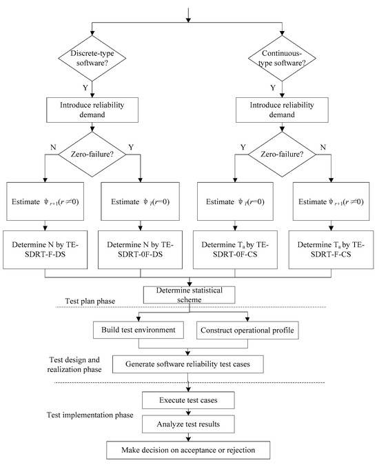
Figure 5. The framework of SRDT with introduced TE.

(1)

Identify the type of software, discrete-type software or continuous-type software.

(2)

Introduce the given reliability demand according to the maximum failure number $r$, and determine which type of plan to use, zero-failure plan or revealed-failure plan.

(3)

For the zero-failure plan, estimate the value of ${\phi }_T$; for the revealed-failure plan, estimate the value of ${\phi }_{r+1}$.

(4)

For discrete-type software, according to the zero-failure plan or revealed-failure plan, determine the minimum test case number by the TE-SRDT-0F-DS plan or TE-SRDT-F-DS plan, respectively. For continuous-type software, the minimum test time is determined by the TE-SRDT-0F-CS plan or TE-SRDT-F-CS plan.

(5)

Build the testing environment.

(6)

Construct the operational profile and generate the corresponding number of reliability test cases according to Step 4.

(7)

Execute test cases and collect failure data.

(8)

Make decisions on acceptance or rejection.

4. Case Study

4.1. Experimental Setup

We chose the Siemens program suite as the subject program. It is the most commonly used testing suite in the field of software defect localization research. It can be downloaded from SIR (Software Infrastructure Repository http://sir.unl.edu/portal/index.php (accessed on 1 August 2024)).

Researchers at Siemens wanted to learn about the effectiveness of the fault detection coverage criteria. Therefore, they created a base version by manually seeding defects, usually by modifying a single line of code in the program. Their goal was to introduce defects on the basis of existing experiments as much as possible. Ten people were involved in seeding defects, most of them with no knowledge of each other’s work. The result of this effort was the generation of multiple mutation versions for each of Siemens’ seven standard programs, each containing a single defect.

It should be noted that the Siemens program suite is the subject of this example verification, but the model is not restricted to the content of the verification, which is used just because it is widely cited in the field of software testing. This method is applicable to any software.

For each program, the original package contains a certain number of original faults, as shown in the column ”Number of faults” in Table 6. The original file states that each defect can be detected by at least 3~350 test cases in the test pool in the Unix environment. Here, the experimental environment is a Windows operating system and GCC compiler.

Table 6. The features of the Siemens program suite.

No.	Program Name	Number of Code Lines	Number of Faults	Test Pool Size	Software Function Description
1	Totinfo	346	23	1052	Information measurement
2	Schedule1	299	9	2650	Priority scheduling
3	Schedule2	297	10	2710	Priority scheduling
4	Tcas	138	41	1608	Contour line identification
5	Printtoken1	402	7	4130	Lexical analysis
6	Printtoken2	483	10	4115	Lexical analysis
7	Replace	516	32	5542	Pattern replacement

All program information is given in Table 6.

4.2. Experimental Procedure

Here, the experiment focuses on Step 1 to Step 4 shown in Figure 5 to illustrate the application steps of the method proposed in this paper, that is, how to determine the SRDT scheme according to the software type and reliability requirements and obtain the estimate of the TE through the statistical fault injection method so as to obtain an explicit improved method and results. The remaining Step 5 to Step 8 are the same as the traditional software reliability testing methodology, so they are omitted here.

First, we used the “Tcas” program as the subject program and then obtained all test results from the Siemens program suite.

Some of the faults and test cases are selected as our fault pool and test case pool, respectively, denoted as Ep and Tp. The fault pool contains 34 faults and is labeled V1-V34. The test case pool contains 870 test cases and is labeled t1–t870. Then, 15 mutation programs $P^{\prime }$ are constructed, that is, $F=15$. The procedures are described as follows:

Firstly, we adopt the Akiyama model [62] $\widehat{M}$ = 4.86 + 0.018 $\times$ L (where L equals the line of code) to obtain the potential failure number of “Tcas”, $\widehat{M}\approx 7$. Then, we use the Poisson distribution as the uniform distribution of residual faults. Therefore, the probability density function is $P_r(M_i=k)={\displaystyle \frac{{\lambda }^k}{k!}}{e}^{-\lambda }(k=0,1,2,\cdots )$, where $\lambda =7$.

According to the Poisson distribution, 15 numbers are randomly selected: 3, 6, 4, 7, 5, 6, 8, 6, 7, 5, 8, 4, 6, 7, and 7.

The mutation program $P^{\prime }$, which contains the same number of faults as the above random numbers, is selected. The details of the inserted faults of $P^{\prime }$ are shown in Table 7.

Table 7. Mutation programs of the “Tcas” program.

No. of Mutation Program	P1	P2	P3	P4	P5	P6	P7	P8	P9	P10	P11	P12	P13	P14	P15
Random number according to Poisson distribution	3	6	4	7	5	6	8	6	7	5	8	4	6	7	7
Inserted fault number	32	20	20	4	8	39	13	23	39	15	30	1	21	27	7
	9	13	30	2	17	4	28	13	7	8	27	5	9	17	5
	26	30	29	19	25	2	26	16	28	40	32	26	6	32	29
		18	9	11	27	10	4	7	29	27	23	25	7	25	24
		15		26	12	32	1	25	11	23	7		32	1	21
		31		30		26	17	27	27		28		15	13	3
				17			21		30		4			29	12
							29				13

The test set $T$ was used to test the 15 mutation programs, as well as the number of mutation programs $P_i$ in which inserted faults were detected and counted. The TE was estimated by the above approach, and the size of the test set was adjusted until a steady TE value was reached. The test case numbers of the test sets $T$ were set to 100, 150, 200, 250, 300, 350, and 400. The TE value was computed in the cases of the zero-failure scheme and one-revealed-failure (i.e., $r=1$) scheme. Therefore, the number of mutation programs for which at least one defect was detected, denoted as K1, was counted, and the number of mutation programs for which at least two faults were detected, denoted as K2, was counted. The test results and TE estimate values are shown in Table 8.

Table 8. Test results.

Test Case Number	100	150	200	250	300	350	400
K1	1	6	10	13	13	13	13
${\widehat{\phi }}_T=K1/F$	0.067	0.4	0.67	0.87	0.87	0.87	0.87
K2	0	2	3	8	13	13	13
${\widehat{\phi }}_2=K2/F$	0	0.133	0.2	0.533	0.87	0.87	0.87

Table 8 shows that all the estimated TE values tend to be stable, as shown in Figure 6 and Figure 7.

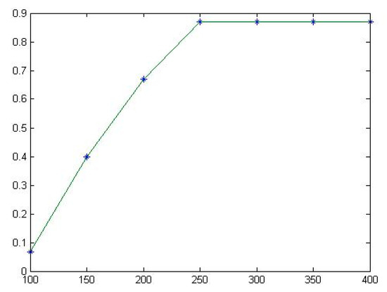
Figure 6. The fitting diagram of ${\widehat{\phi }}_T$ for Tcas.

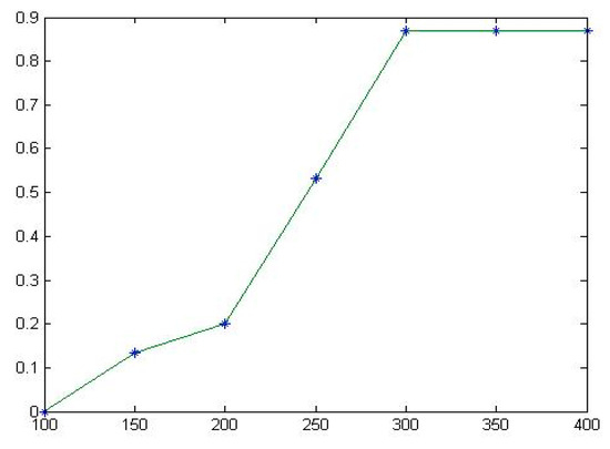
Figure 7. The fitting diagram of ${\widehat{\phi }}_2$ for Tcas.

According to the TE values in Table 7, we present the TE-SRDT-0F-DS and TE-SRDT-F-DS (in the case of failure number $r=1$) schemes. The results are shown in Table 9.

Table 9. The minimum test case number of the TE-SRDT for the “Tcas” program.

Program Name	Zero-Failure Test Plan				$\mathbf{Test} \mathbf{Plan} \mathbf{with} \mathbf{Revealed} \mathbf{Failure} \mathit{r}=1$
	${\widehat{\mathit{\phi }}}_{\mathit{T}}$	${\mathit{N}}_{\mathit{T}}$	$\mathit{N}$	EF	${\widehat{\mathit{\phi }}}_2$	${\mathit{N}}_{\mathit{T}}$	$\mathit{N}$	EF
Tcas	0.87	25,648	46,049	44.3%	0.87	42,166	66,380	36.5%

Notes: In Table 8, $N_T$ stands for the minimum test case number considering TE, $N$ stands for the minimum test case number without considering TE, and EF indicates the test case number reduction percentage.

From Table 9, the experimental results show that within the same limitations of reliability requirements and confidence levels, this approach gives the required number of tests with no failures, 25,648, compared to 46,049 with the traditional method, which greatly reduces the number of test cases required, but achieves the same level of confidence and reliability. When one failure is allowed, this approach gives a number of 42,166 compared to 66,380 for the traditional approach, so this approach greatly reduces the number of test cases required while achieving the same level of confidence and reliability. That is, the proposed method can effectively reduce the number of test cases, i.e., accelerate the testing process and improve the efficiency of the SRDT.

The test results for the other six programs are shown in Table 10 and Table 11. The corresponding fitting diagrams are shown in Figure 8, Figure 9, Figure 10, Figure 11, Figure 12, Figure 13, Figure 14 and Figure 15.

Table 10. All test results for the Siemens program suite.

No.	Program Name	$\widehat{\mathit{M}}$	Ep’ Size	Tp’ Size	${\widehat{\mathit{\phi }}}_{\mathit{T}}$ Stable Value with Zero-Failure		${\widehat{\mathit{\phi }}}_2$ Stable Value with Revealed Failures
					The Minimum Test Case Number	${\widehat{\mathit{\phi }}}_{\mathit{T}}$	The Minimum Test Case Number	${\widehat{\mathit{\phi }}}_2$
1	Totinfo	3	20	560	250	0.733	250	0.333
2	Schedule1	1	8	2,046	1,200	0.467	-	-
3	Schedule2	1	9	2,528	1,600	0.6	-	-
4	Tcas	7	34	870	250	0.87	300	0.87
5	Printtoken1	1	6	3,715	1,000	0.533	-	-
6	Printtoken2	1	9	3,053	2,000	0.615	-	-
7	Replace	4	28	3,639	2,800	0.8	2,000	0.667

Table 11. Effect of TE on the minimum number of test cases for the Siemens program suite.

Program Name	Zero-Failure Scheme				Scheme with Failure Number r = 1
	${\widehat{\mathit{\phi }}}_{\mathit{T}}$	${\mathit{N}}_{\mathit{T}}$	$\mathit{N}$	EF	${\widehat{\mathit{\phi }}}_2$	${\mathit{N}}_{\mathit{T}}$	$\mathit{N}$	EF
Totinfo	0.733	32,595	46,049	29.2%	0.333	61,448	66,380	7.43%
Schedule1	0.467	38,558	46,049	16.3%	-	-	-	-
Schedule2	0.6	35,287	46,049	23.4%	-	-	-	-
Tcas	0.87	25,398	46,049	44.8%	0.87	41,866	66,380	36.9%
Printtoken1	0.533	37,436	46,049	18.7%	-	-	-	-
Printtoken2	0.615	34,887	46,049	24.2%	-	-	-	-
Replace	0.8	27,156	46,049	41.0%	0.667	51,545	66,380	22.3%

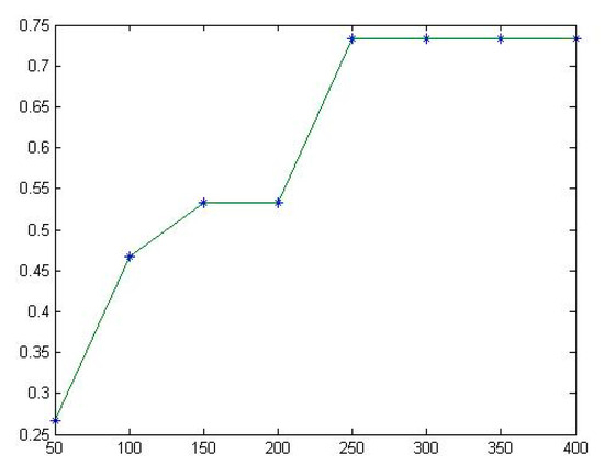
Figure 8. The fitting diagram of ${\widehat{\phi }}_T$ for Totinfo.

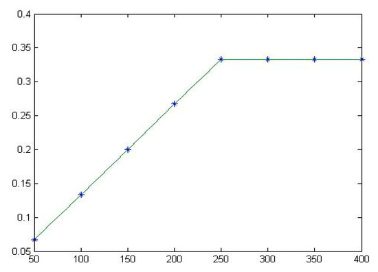
Figure 9. The fitting diagram of ${\widehat{\phi }}_2$ for Totinfo.

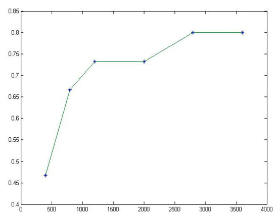
Figure 10. The fitting diagram of ${\widehat{\phi }}_T$ for Replace.

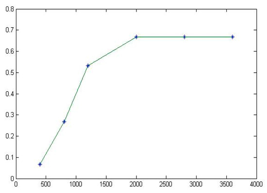
Figure 11. The fitting diagram of ${\widehat{\phi }}_2$ for Replace.

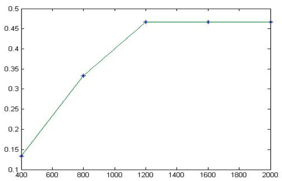
Figure 12. The fitting diagram of ${\widehat{\phi }}_T$ for Schedule1.

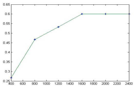
Figure 13. The fitting diagram of ${\widehat{\phi }}_T$ for Schedule2.

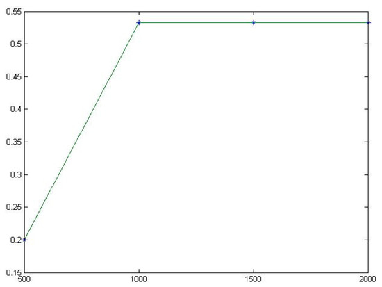
Figure 14. The fitting diagram of ${\widehat{\phi }}_T$ for Printtoken1.

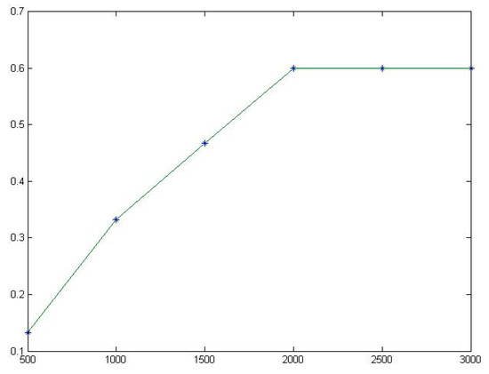
Figure 15. The fitting diagram of ${\widehat{\phi }}_T$ for Printtoken2.

From Table 10 and Table 11, the method gives the same conclusions for the other six programs. In addition, it can be seen that the TE of different programs is different, and the higher the TE, the smaller the number of test cases required, that is, the greater the increase in test efficiency. This once again proves that it is not reasonable to perform the same number of statistical tests on all software without distinction.

4.3. Discussion of Experimental Results

(1)

Impact of TE on SRDT plan

Take TCAS for example, which is shown in Table 8.

i.

If TE and prior information are not considered, the required number of tests with no failures is $N=\left[\ln \left(1-C\right)/\ln (1-p_0)\right]$= 46,049 for $p_0=0.0001$ and $C=0.99$. For ${\widehat{\phi }}_T=0.87$, for the given $(p_0,C)$ = $(0.0001,0.99)$, according to Equation (43), then the required number of tests with no failures is $N$ = 25,398, and the test case number reduction percentage is 44.8%.

ii.

If TE and prior information are not considered, the required number of tests with one failure is $N$ = 66,380 for the given $(p_0,C)$ = $(0.0001,0.99)$. For ${\widehat{\phi }}_T=0.87$, then the required number of tests with one failure is $N$ = 41,866, and the test case number reduction percentage is 36.9%.

The same conclusions can be found in the other six programs, which are shown in Table 10. Thus, the experimental results show that within the same limitation of requirements and confidence levels, this approach can effectively reduce the number of test cases, i.e., accelerate the test process and improve the efficiency of the SRDT.

(2)

Stability of TE

From Table 8 and Table 10, it can be seen that when the test set T is continuously updated to make the test set larger and larger, its ability to find injected defects becomes stronger, and TE eventually tends to a stable value.

i.

For the TCAS program, when the number of test cases in the test set is 100, the TE is estimated to be 0.067. When the numbers of test cases in the test set is 150 and 200, the TE is estimated to be 0.4 and 0.67, respectively. When the number of test cases in the test set is 250, the TE is estimated to be 0.87, and then it stabilizes at 0.87. When the test case set contains more than 250 test cases, e.g., 300, 350, or 400 test cases, the TE tends to stabilize at 0.87.

ii.

For the Totinfo program, when the numbers of test cases in the test set is 50, 100, 150, and 200, the TE is estimated to be 0.267, 0.467, 0.533, and 0.533, respectively. When the number of test cases in the test set is 250, the TE is estimated to be 0.733, and then it stabilizes at 0.733. When the test case set contains more than 250 test cases, e.g., 300, 350, or 400 test cases, the TE tends to be stable at 0.733.

The same conclusions can be found in the other five programs, which are shown in Table 10 and Figure 8, Figure 9, Figure 10, Figure 11, Figure 12, Figure 13, Figure 14 and Figure 15. Therefore, the experimental results indicate that TE has a certain degree of stability and will eventually approach a stable value.

(3)

Additional comments

In this paper, we believe that the original program $P$ is a faultless version of the program $P^G$ with some defects. Then, we create a large number of mutation versions $P^{\prime }$ through fault injection technology, which are also $P^G$ version-based programs with random defects $F{S}_i$. Thus, it can be assumed that the mutation program $P^{\prime }$ contains defects with the same statistical distribution characteristics as the original program. The test on the mutation program $P^{\prime }$ is considered to be similar to the test on the original program.

However, the reduction in the number of test cases is different for different programs. This is because different programs have different testability, which is an intrinsic quality property of the program, but is reflected in the outward manifestation of TE of the test set. For example, if some defects of a program require more test cases than others, the testability of a program with the former defects is essentially lower than that of a program with the latter. This confirms that it is not appropriate for programs with different levels of testability to use the same number of statistical test cases to reach the same expected reliability level.

5. Conclusions and Future Work

This paper extends the research on the introduction of TE to the SDRT approach, as it provides a quantitative assessment of testability as an indicator of the statistical power of the test set. First, we suggest the principle of the SDRT approach introducing TE in the case of zero-failure by modeling the program space division according to the test set, and then propose a detailed form of determining the test effort based on the Bayesian prior distribution. Second, we present the principle and determining form of the SDRT approach introducing TE in the case of revealed failures, which is considered an ongoing issue in many studies. Then, the estimation method of TE by statistical fault injection is studied further by combining the different cases of zero-failure and revealed failures, and the uniform framework of the improved SRDT is proposed for both failure conditions and different software types, i.e., discrete-type software and continuous-type software. Finally, a case study on the Siemens program suite is presented to describe the implementation procedures and validate the testing efficiency of the improved testing method.

Future work should address the limitations of our approach to enhance its effectiveness. Apparently, the additional testing effort for generating prior test cases and estimating the value of TE are some disadvantages of the improved testing approach. Therefore, we should consider the balance between profits (testing efficiency improvement) and costs (i.e., additional testing effort) according to the actual conditions. Moreover, the detailed statistical fault injection method needs to be studied further, and additional hypotheses should be discussed and formulated further.

References

- Salama, M.; Bahsoon, R. Analysing and modelling runtime architectural stability for self-adaptive software. J. Syst. Softw. 2017, 133, 95–112. [Google Scholar] [CrossRef]
- Li, M.; Zhang, W.; Hu, Q.; Guo, H.; Liu, J. Design and Risk Evaluation of Reliability Demonstration Test for Hierarchical Systems with Multilevel Information Aggregation. IEEE Trans. Reliab. 2016, 66, 135–147. [Google Scholar] [CrossRef]
- Zheng, H.; Yang, J.; Zhao, Y. Reliability demonstration test plan for degraded products subject to Gamma process with unit heterogeneity. Reliab. Eng. Syst. Saf. 2023, 240, 1.1–1.15. [Google Scholar] [CrossRef]
- Sandoh, H. Reliability demonstration testing for software. IEEE Trans. Reliab. 1991, 40, 117–119. [Google Scholar] [CrossRef]
- Feller, W. An Introduction to Probability Theory and Its Applications. Am. Math. Mon. 1971, 59, 265. [Google Scholar] [CrossRef]
- Thayer, T.A.; Lipow, M.; Nelson, E.C. Software Reliability; North-Holland: Amsterdam, The Netherlands, 1978. [Google Scholar]
- Miller, K.W.; Morell, L.J.; Noonan, R.E. Estimating the probability of failure when testing reveals no failures. IEEE Trans. Softw. Eng. 1992, 18, 33–43. [Google Scholar] [CrossRef]
- Mann, N.R.; Schafer, R.E.; Singpurwalla, N.D. Methods for Statistical Analysis of Reliability and Life Data; Wiley: New York, NY, USA, 1974. [Google Scholar]
- Martz, H.F.; Waller, R.A. A Bayesian zero-failure (BAZE) reliability demonstration testing procedure. J. Qual. Technol. 1979, 11, 128–138. [Google Scholar] [CrossRef]
- Rahrouh, M. Bayesian Zero-Failure Reliability Demonstration; Durham University: Durham, NC, USA, 2005. [Google Scholar]
- MIL-HDBK-781A: Reliability Test Methods, Plans and Environments; US Department of Defence: Washington, DC, USA, 1996.
- Chen, G. Reliability test and estimation for 0-1 binary systems with unknown distributions. Reliab. Rev. 1995, 15, 19–25. [Google Scholar]
- Tal, O.; MoCollin, C.; Bendell, A. Reliability Demonstration for Safety-Critical Systems. IEEE Trans. Reliab. 2001, 50, 194–203. [Google Scholar] [CrossRef]
- Tal, O.; Bendell, A.; Mccollin, C. Comparison of methods for calculating the duration of software reliability demonstration testing, particularly for safety-critical systems. Qual. Reliab. Eng. Int. 2000, 16, 59–62. [Google Scholar] [CrossRef]
- Kececioglu, D. Reliability and Life Testing Handbook; Prentice Hall: Englewood Cliffs, NJ, USA, 1993. [Google Scholar]
- Malaiya, Y.K.; Li, N.; Bieman, J.; Karcich, R.; Skibbe, B. The relation between software test coverage and reliability. In Proceedings of the Fifth IEEE International Symposium on Software Reliability Engineering, Monterey, CA, USA, 6–9 November 1994; pp. 186–195. [Google Scholar]
- Chen, H.; Lyu, M.R.; Wong, W.E. An empirical study of the correlation between code coverage and reliability estimation. In Proceedings of the Third IEEE International Software Metrics Symposium, Berlin, Germany, 25–26 March 1996; pp. 133–141. [Google Scholar]
- Bertolino, A.; Strigini, L. On the use of testability measures for dependability assessment. IEEE Trans. Softw. Eng. 1996, 22, 97–108. [Google Scholar] [CrossRef][Green Version]
- Yang, M.C.K.; Wong, W.E.; Pasquini, A. Applying testability to reliability estimation. In Proceedings of the Ninth International Symposium on Software Reliability Engineering, Paderborn, Germany, 4–7 November 1998; pp. 90–99. [Google Scholar]
- Voas, J.M.; Miller, K.W. Software Testability: The New Verification. IEEE Softw. 1995, 12, 17–28. [Google Scholar] [CrossRef]
- ANSI/IEEE Standard 610.12-1990; IEEE standard Glossary of software Engineering Terminology. IEEE Press: New York, NY, USA, 1990.
- ISO/IEC25010; Systems and Software Engineering—Systems and Software Quality Requirements and Evaluation (SQuaRE)-System and Software Quality Models. International Standard Organization: Geneva, Switzerland, 2011.
- Hamlet, D.; Voas, J. Faults on its Sleeve: Amplifying Software Reliability Testing. In Proceedings of the 1993 ACM SIGSOFT International Symposium on Software Testing and Analysis, Cambridge, MA, USA, 28–30 June 1993; pp. 89–98. [Google Scholar]
- Chen, W.; Untch, R.H.; Gregg, R.H. Can fault-exposure-potential estimates improve the fault detection abilities of test suites? J. Softw. Test. Verif. Reliab. 2002, 4, 197–218. [Google Scholar] [CrossRef]
- Kuball, S.; May, J. Test-adequacy and statistical testing combining different properties of a test-set. In Proceedings of the 15th International Symposium on Software Reliability Engineering, Saint-Malo, Bretagne, France, 2–5 November 2004; pp. 161–172. [Google Scholar]
- Kuball, S.; Hughes, G.; May, J. The Effectiveness of Statistical Testing when Applied to Logic Systems. Saf. Sci. 2004, 42, 369–383. [Google Scholar] [CrossRef]
- Kuball, S.; May, J.H.R. A discussion of statistical testing on a safety-related application. Proc. Inst. Mech. Eng. Part O J. Risk Reliab. 2007, 221, 121–132. [Google Scholar] [CrossRef]
- Gough, H.; Kuball, S. Application of Statistical Testing to the Data Processing and Control System for the Dungeness B Nuclear Power Plant (Practical Experience Report). In Proceedings of the 2014 Tenth European Dependable Computing Conference, Newcastle, UK, 13–16 May 2014. [Google Scholar] [CrossRef]
- Li, Q.-Y.; Li, H.-F.; Wang, J. Study on the relationship between software test effectiveness and software reliability demonstration testing. In Proceedings of the 2010 3rd International Conference on Computer Science and Information Technology, Wuxi, China, 4–6 June 2010. [Google Scholar] [CrossRef]
- Ma, Z.; Zhang, W.; Wu, W.; Wang, J.; Liu, F. Overview of Software Reliability Demonstration Testing Research Method. J. Ordnance Equip. Eng. 2019, 40, 118–123. [Google Scholar]
- Tal, O. Software Dependability Demonstration for Safety-Critical Military Avionics System by Statistical Testing. Ph.D. Thesis, Nottingham Trent University, Nottingham, UK, 1999. [Google Scholar]
- Cho, C.K. An Introduction to Software Quality Control; Wiley: New York, NY, USA, 1980. [Google Scholar]
- Sawada, K.; Sandoh, H. Continuous model for software reliability demonstration testing considering damage size of software failures. Math. Comput. Model. 2000, 31, 321–326. [Google Scholar] [CrossRef]
- Chan, H.A. Accelerated stress testing for both hardware and software. In Proceedings of the Annual Reliability and Maintainability Symposium, Los Angeles, CA, USA, 26–29 January 2004; pp. 346–351. [Google Scholar]
- Tang, D.; Hecht, H. An approach to measuring and assessing dependability for critical software systems. In Proceedings of the 8th International Symposium on Software Reliability Engineering, Albuquerque, NM, USA, 2–5 November 1997; pp. 192–202. [Google Scholar]
- Hecht, M.; Hecht, H. Use of importance sampling and related techniques to measure very high reliability software. In Proceedings of the Aerospace Conference Proceedings, Big Sky, MT, USA, 18–25 March 2000; pp. 533–546. [Google Scholar]
- Chen, M.H.; Lyu, M.R.; Wong, W.E. Effect of code coverage on software reliability measurement. IEEE Trans Reliab. 2001, 50, 165–170. [Google Scholar] [CrossRef]
- Bishop, P.G. Estimating residual faults from code coverage. In Proceedings of the 21st International Conference on Computer Safety, Reliability and Security, Catania, Italy, 10–13 September 2002; pp. 10–13. [Google Scholar]
- ISO/IEC 9126-1:2001; Software Quality Attributes, Software Engineering-Product Quality, Part 1:Quality model. International Organization of Standardization: Geneva, Switzerland, 2001.
- Voas, J.M. Factors that Affect Software Testability. In Proceedings of the 9th Pacific Northwest Software Quality Conference, Portland, OR, USA, 7–8 October 1991; pp. 235–247. [Google Scholar]
- Jungmayr, S. Improving Testability of Object-Oriented Systems. Ph.D. Thesis, de-Verlag im Internet Gmbh, Berlin, Germany, 2004. [Google Scholar]
- Gao, J.; Shih, M.C. A Component Testability Model for Verification and Measurement. In Proceedings of the 29th annual International Computer Software and Application Conferences(COMPSAC’ 2005), Edinburgh, UK, 26–28 July 2005; pp. 211–218. [Google Scholar]
- Freedman, R.S. Testability of software components. IEEE Trans. Softw. Eng. 1991, 17, 553–564. [Google Scholar] [CrossRef]
- McGregor, J.; Srinivas, S. A Measure of Testing Effort. In Proceedings of the Conference on Object-Oriented Technologies, Toronto, ON, Canada, 17–21 June 1996. [Google Scholar]
- Richard, B.; Monica, M. Measures of testability as a basis for quality assurance. Softw. Eng. J. 1990, 5, 86–92. [Google Scholar]
- Nguyen, T.B.; Delaunay, M.; Robach, C. Testability Analysis For Software Components. In Proceedings of the International Confefence On Software Maintenance’2002 (ICSM’02), Montreal, QC, Canada, 3–6 October 2002; pp. 422–429. [Google Scholar]
- Lo, B.W.; Shi, H. A preliminary Testability Model for Object-Oriented Software. In Proceedings of the International Conference on Software Engineering: Education & Practice, Dunedin, New Zealand, 26–29 January 1998; pp. 330–337. [Google Scholar]
- Sohn, S.; Seong, P. Quantitative evaluation of safety critical software tastability based on fault tree analysis and entropy. J. Syst. Softw. 2004, 73, 351–360. [Google Scholar] [CrossRef]
- Khoshgoftaar, T.M. Predicting testability of program modules using a neural network. In Proceedings of the 3rd IEEE Symposium on Application Specific Systems and Software Engineering Technique, Richardson, TX, USA, 24–25 March 2000; pp. 57–62. [Google Scholar]
- Bruntink, M.; Deursen, A.V. Predicting class testability using object-oriented metrics. In Proceedings of the 4th International Workshop on Source Code Analysis and Manipulation (SCAM’04), Chicago, IL, USA, 15–16 September 2004. [Google Scholar]
- Voas, J.M. PIE: A Dynamic Failure-Based Technique. IEEE Trans. Softw. Eng. 1992, 18, 717. [Google Scholar] [CrossRef]
- Lin, J.C.; Lin, S.W.; Ian-Ho. An estimated method for software testability measurement. In Proceedings of the 8th International WorkShop on Software Technology and Engineering Practices (STEP’97), London, UK, 14–18 July 1997. [Google Scholar]
- Frankl, P.G.; Iakounenko, O. Further empirical studies of test effectiveness. In Proceedings of the 6th ACM SIGSOFT International Symposium on Foundations of Software Engineering, Lake Buena Vista, FL, USA, 3–5 November 1998; ACM Press: New York, NY, USA, 1998; pp. 153–162. [Google Scholar]
- Hutchins, M.; Foster, H.; Goradia, T.; Ostrand, T. Experiments on the effectiveness of dataflow and controlflow-based test adequacy criteria. In Proceedings of the 16th International Conference on Software Engineering, Sorrento, Italy, 16–21 May 1994; IEEE Press: New York, NY, USA, 1994; pp. 191–200. [Google Scholar]
- Frankl, P.G.; Weiss, S.N. An experimental comparison of the effectiveness of branch testing and data flow testing. IEEE Trans Softw. Eng. 1993, 19, 774–787. [Google Scholar] [CrossRef]
- Stott, D.T.; Ries, G.; Hsueh, M.C.; Iyer, R.K. Dependability analysis of a high-speed net work using software-implemented fault injection and simulated fault. IEEE Trans Comput. 1998, 47, 108–119. [Google Scholar] [CrossRef]
- Hamlet, R. Testing programs with the aid of a compiler. IEEE Trans. Softw. Eng. 1977, 3, 279–290. [Google Scholar] [CrossRef]
- DeMillo, R.; Lipton, R.; Sayward, F. Hints on test data selection: Help for the practicing programmer. IEEE Comput. 1978, 11, 34–43. [Google Scholar] [CrossRef]
- Howden, W.E. Weak mutation testing and completeness of test sets. IEEE Trans. Softw. Eng. 1982, 8, 371–379. [Google Scholar] [CrossRef]
- Leveugle, R.; Calvez, A.; Maistri, P.; Vanhauwaert, P. Statistical Fault Injection: Quantified Error and Confidence. In Proceedings of the Design, Automation & Test in Europe Conference & Exhibition, Nice, France, 20–24 April 2009; pp. 502–506. [Google Scholar]
- Leveugle, R.; Calvez, A.; Maistri, P.; Vanhauwaert, P. Precisely Controlling the Duration of Fault Injection Campaigns: A Statistical View. In Proceedings of the 2009 4th International Conference on Design & Technology of Integrated Systems in Nanoscal Era, Cairo, Egypt, 6–9 April 2009; pp. 149–154. [Google Scholar]
- Nanda, M.; Jayanthi, J.; Rao, S. An Effective Verification and Validation Strategy for Safety-Critical Embedded Systems. Int. J. Softw. Eng. Appl. 2013, 4, 123–142. [Google Scholar] [CrossRef]
Disclaimer/Publisher’s Note: The statements, opinions and data contained in all publications are solely those of the individual author(s) and contributor(s) and not of MDPI and/or the editor(s). MDPI and/or the editor(s) disclaim responsibility for any injury to people or property resulting from any ideas, methods, instructions or products referred to in the content. |
© 2024 by the authors. Licensee MDPI, Basel, Switzerland. This article is an open access article distributed under the terms and conditions of the Creative Commons Attribution (CC BY) license (https://creativecommons.org/licenses/by/4.0/).