Symmetry, Asymmetry and Studentized Statistics

Abstract

Inferences on the location parameter $\lambda$ in location-scale families can be carried out using Studentized statistics, i.e., considering estimators $\tilde{\lambda }$ of $\lambda$ and $\tilde{\delta }$ of the nuisance scale parameter $\delta$, in a statistic $T=g(\tilde{\lambda },\tilde{\delta })$ with a sampling distribution that does not depend on $(\lambda ,\delta )$. If both estimators are independent, then T is an externally Studentized statistic; otherwise, it is an internally Studentized statistic. For the Gaussian and for the exponential location-scale families, there are externally Studentized statistics with sampling distributions that are easy to obtain: in the Gaussian case, Student’s classic t statistic, since the sample mean $\tilde{\lambda }=\overline{X}$ and the sample standard deviation $\tilde{\delta }=S$ are independent; in the exponential case, the sample minimum $\tilde{\lambda }=X_{1:n}$ and the sample range $\tilde{\delta }=X_{n:n}-X_{1:n}$, where the latter is a dispersion estimator, which are independent due to the independence of spacings. However, obtaining the exact distribution of Student’s statistic in non-Gaussian populations is hard, but the consequences of assuming symmetry for the parent distribution to obtain approximations allow us to determine if Student’s statistic is conservative or liberal. Moreover, examples of external and internal Studentizations in the asymmetric exponential population are given, and an ANalysis Of Spacings (ANOSp) similar to an ANOVA in Gaussian populations is also presented.

1. Introduction

Let $\mathit{X}$ $=\left(X_1,\dots ,X_n\right)$ be a random sample from a population $X\sim \mathrm{Gaussian}(\mu ,\sigma )$. If the location parameter $\mu$ and the scale parameter $\sigma$ are unknown, the unbiased estimators $\tilde{\mu }=\overline{X}={\displaystyle \frac{1}{n}}{\sum }_{k=1}^n{X}_k\sim \mathrm{Gaussian}\left(\mu ,\frac{\sigma }{\sqrt{n}}\right)$ and ${\tilde{\sigma }}^2=S^2={\displaystyle \frac{1}{n-1}}{\sum }_{k=1}^n{(X_k-\overline{X})}^2$, with ${\displaystyle \frac{(n-1)S^2}{{\sigma }^2}}\sim {\chi }_{n-1}^2$, can be used to estimate these parameters.

The distribution of the estimator $\overline{X}$ depends on the nuisance parameter $\sigma$, which is a problem for making inferences on the location parameter $\mu$. Student’s [1] pathbreaking paper has shown that the statistic

$$t_{n-1}=\sqrt{n}{\displaystyle \frac{\overline{X}-\mu }{S}}$$

(1)

has a distribution that does not depend on the nuisance scale parameter, since its probability density function is

$$f_{t_{n-1}}\left(t\right)={\displaystyle \frac{1}{B\left(\frac{1}{2},\frac{n-1}{2}\right)}}{\displaystyle \frac{1}{\sqrt{n-1}{\left(1+\frac{t^2}{n-1}\right)}^{n/2}}}{\mathbb{I}}_{\mathbb{R}}\left(t\right),$$

(2)

where $B(p,q)={\int }_0^1{x}^{p-1}{(1-x)}^{q-1}\mathrm{d}x$, $p,q>0$, is Euler’s Beta function. The probability density function defined in (2) is for a random variable with Student’s distribution with $n-1$ degrees of freedom. Basically, the “Studentization” defined in (1), as opposed to the common standardization ${\displaystyle \frac{\overline{X}-\mu }{\sigma /\sqrt{n}}}$, uses the estimators of the parameter of interest (location) and of the nuisance parameter, so that the sampling distribution of $t_{n-1}=g(\overline{X},S)$ does not depend on the location parameter $\mu$ or on the nuisance parameter $\sigma$, thus being a pivot statistic that can be used for inferences on $\mu$.

However, Student’s exceptional result depends heavily on the fact that in the location-scale Gaussian family, $\overline{X}$ and $S^2$ are independent random variables, which is an exclusive property of the Gaussian family. This characterization of the Gaussian distribution appeared in Geary’s work [2], and has been proved, independently, by Darmois [3] and by Skitovich [4]. Additionally, in the context of the Koopman–Darmois–Pitman k-parameter exponential family [5,6,7], the Gaussian family is the only one with support $\mathbb{R}$ and with a pair of sufficient statistics for $(\mu ,\sigma )$, namely $\left({\sum }_{k=1}^n{X}_k,{\sum }_{k=1}^n{X}_k^2\right)$, which captures all available information in the sample to estimate these two parameters.

When working with samples from non-Gaussian location-scale families, the dependence structure between the sample mean ${\overline{X}}_n={\displaystyle \frac{1}{n}}{\sum }_{k=1}^n{X}_k$ and the sum of squares $S{S}_n={\sum }_{k=1}^n{(X_k-{\overline{X}}_n)}^2=(n-1)S_n^2$ is hard to discern, except for the special case $n=2$ (note that an index n is now being used to emphasize the size of the random sample). For $n>2$, the computation of the probability density function of Student’s statistic

$$T_{n-1}=\sqrt{n(n-1)}{\displaystyle \frac{{\overline{X}}_n-\lambda }{\sqrt{S{S}_n}}}$$

(3)

is a more difficult problem to handle. In Section 2, the joint probability density function of $({\overline{X}}_n,S{S}_n)$ is investigated in a general context, i.e., not restricted to the Gaussian family. Its explicit expression for $n=2$ is given in Section 2.1, and examples for the probability density function of $T_1$, i.e., for $n=2$ in (3), for several symmetric parent distributions are given in Section 2.2. For $n\ge 3$, a recurrence formula for the joint probability density function of $({\overline{X}}_n,S{S}_n)$ is obtained in Section 2.3, and a detailed study of the recurrence formula for the Gaussian case is seen in Section 2.4.

An interesting alternative for Studentization was proposed in Logan et al.’s work [8], where a self-normalized statistic $W_{n-1}^{\ast }={\displaystyle \frac{{\sum }_{k=1}^n{X}_k}{{\left({\sum }_{k=1}^n{\left|X_k\right|}^{\alpha }\right)}^{1/\alpha }}}$ was considered, especially when X has heavier tails than the Gaussian law, and it is in the domain of attraction of a stable law for sums with index $\alpha \in (0,2)$. Peña et al.’s [9] monograph on self-normalized processes is a thorough overview, with Chapter 15 dealing with the classical t-statistic and Studentized statistics.

Another interesting fact is that Efron [10] showed that $T_{n-1}\stackrel{d}{=}{t}_{n-1}$ when a rotational symmetry of the unit vector $\mathit{U}={\displaystyle \frac{\mathit{X}}{\parallel \mathit{X}\parallel }}=\left({\displaystyle \frac{X_1}{\parallel \mathit{X}\parallel }},\dots ,{\displaystyle \frac{X_n}{\parallel \mathit{X}\parallel }}\right)$ over the surface of the unit sphere in the Euclidean n-space $E^n$ is assumed. However, Efron [10] pointed out the following:

Unfortunately the usual sampling procedures almost never yield rotational symmetry for the normalized vector $\mathit{U}$ except in the case $X\sim \mathrm{Gaussian}(0,{\sigma }^2)$.

Efron also stated that “A very special “lucky” case is given in Section 9, namely Inverted normal error for $n=2$. It is possible to construct examples where $T_n$ is t-distributed with n degrees of freedom, without $\mathit{U}$ having rotational symmetry”. Efron’s [10] pioneering work also investigated the consequences, in what regards Student’s statistic, by assuming weaker orthant symmetry, i.e., when the random vector $\mathit{U}=\left(U_1,\dots ,U_n\right)$ has the same distribution as ${\mathit{U}}_{\mathit{\delta }}=\left({\delta }_1{U}_1,\dots ,{\delta }_n{U}_n\right)$ for every choice of ${\delta }_i=\pm 1$, $i=1,2,\dots ,n$.

This led us to observe, in Section 2.4, that the joint probability density function of $({\overline{X}}_n,S{S}_n)$, in the exceptional rotational symmetry of the Gaussian case, is proportional to the product of n Gaussian$(0,\sigma )$ probability density functions, computed at some special points that form a symmetric arithmetic progression with a null sum and a sum of squares equal to one.

In Section 3, we shall investigate the simplifications that result from an additional symmetry assumption, namely when the joint probability density function of $({\overline{X}}_n,S{S}_n)$ is proportional to the product of n probability density functions of X, as in the Gaussian case. The approximation obtained from the smoothness hypothesis 1 (Section 3.2) is further investigated in Section 3.3 for the worst case possible, i.e., uniform distribution (see Hendriks et al. [11]), by comparing the approximate expression for $T_2$ with the exact distribution given by Perlo [12] for a $\mathrm{Uniform}(-1,1)$ parent.

Aside from the Gaussian family, the exponential location-scale family is also a remarkable member of the Koopman–Darmois–Pitman exponential family. It is the only member of this family with support in a half-line $[\lambda ,\infty )$ and with a pair of sufficient statistics to estimate $(\lambda ,\delta )$, namely $(X_{1:n},{\overline{X}}_n-X_{1:n})$, where $X_{k:n}$, $k=1,\dots ,n$, denotes the k-th order statistic of the random sample $(X_1,\dots ,X_n)$.

Moreover, the spacings $X_{k:n}-X_{k-1:n}\sim \mathrm{Exponential}\left(0,{\displaystyle \frac{1}{n+1-k}}\right)$, $k=1,\dots ,n$, are independent, with the convention $X_{0:n}=\lambda$. This property characterizes the exponential distribution, and it is a consequence of Pexider’s [13] functional equation $f(x+y)={\varphi }_1\left(x\right){\varphi }_2\left(y\right)$, which is an extension of Cauchy’s functional equation, with the solution $f\left(x\right)=k_1{\mathrm{e}}^{k_{2}x}$.

Using the independence of the spacings of the exponential model, we shall also obtain in Section 4 the probability density function of some externally and internally Studentized statistics, according to David’s [14] definition, for inferences on the exponential location parameter. The independence of spacings is further used to compare the location parameters of two exponential populations in Section 4.4, and also to establish an ANalysis Of Spacings (ANOSp), similar to a one-way ANOVA in Gaussian populations, which is presented in Section 4.5. A Satterthwaite [15] approximation for the case of unequal dispersions is given in Section 4.6.

Finally, Section 5 summarizes the main findings regarding approximate solutions for non-Gaussian symmetric populations and for a very asymmetric exponential population, either for exact solutions resulting from the independence of spacings or for approximate solutions for inferences on the comparison of $k\ge 2$ location parameters without assuming equal dispersions.

2. Joint Probability Density Function of $({\overline{\mathit{X}}}_{\mathit{n}},{\mathit{SS}}_{\mathit{n}})$ and Probability Density Function of ${\mathit{T}}_{\mathit{n}-\mathbf{1}}$

Let $\mathit{X}=\left(X_1,\dots ,X_n\right)$ be a random sample of size n from a population X. If $X\sim \mathrm{Gaussian}(\mu ,\sigma )$, then from the independence of ${\overline{X}}_n$ and $S{S}_n$, the joint probability density function of $({\overline{X}}_n-\mu ,S{S}_n)$ is

$$\begin{array}{cc}\hfill f_{({\overline{X}}_n-\mu ,S{S}_n)}(w,s)& =f_{{\overline{X}}_n-\mu }\left(w\right)f_{S{S}_n}\left(s\right)\hfill \\ & ={\displaystyle \frac{1}{\sqrt{2\pi }(\sigma /\sqrt{n})}}{\mathrm{e}}^{-{\displaystyle \frac{1}{2}}{\left({\displaystyle \frac{w}{\sigma /\sqrt{n}}}\right)}^2}{\displaystyle \frac{s^{\frac{n-1}{2}-1}{\mathrm{e}}^{-\frac{s}{2{\sigma }^2}}}{{\left(2{\sigma }^2\right)}^{\frac{n-1}{2}}\Gamma \left(\frac{n-1}{2}\right)}}{\mathbb{I}}_{\mathbb{R}\times {\mathbb{R}}^{+}}(w,s),\hfill \end{array}$$

(4)

where $\Gamma \left(\alpha \right)={\int }_0^{\infty }{x}^{\alpha -1}{\mathrm{e}}^{-x}\mathrm{d}x$, $\alpha >0$, is Euler’s Gamma function.

2.1. Joint Probability Density Function of $({\overline{X}}_2,S{S}_2)$

The independence of ${\overline{X}}_n$ and $S{S}_n$ does not hold for a non-Gaussian population X. However, for samples of size $n=2$, it is easy to obtain the probability density function of Student’s statistic $T_1$.

Since

$${\overline{X}}_2={\displaystyle \frac{X_1+X_2}{2}}\mathrm{and}S{S}_2={\displaystyle \frac{{(X_1-X_2)}^2}{2}},$$

it follows that if $X_1\ge X_2$, then

$$X_1={\overline{X}}_2+\sqrt{{\displaystyle \frac{S{S}_2}{2}}}\mathrm{and}{X}_2={\overline{X}}_2-\sqrt{{\displaystyle \frac{S{S}_2}{2}}},$$

with a similar result also holding true if $X_1<X_2$, namely $X_1={\overline{X}}_2-\sqrt{{\displaystyle \frac{S{S}_2}{2}}}$ and $X_2={\overline{X}}_2+\sqrt{{\displaystyle \frac{S{S}_2}{2}}}$. Therefore, if we denote $f_X$ the probability density function of X, as the absolute value for the Jacobian determinant of both transformations is $\left|J\right|={\displaystyle \frac{1}{\sqrt{2S{S}_2}}}$, then the joint probability density function of $({\overline{X}}_2,S{S}_2)$ is

$$\begin{array}{cc}\hfill f_{({\overline{X}}_2,S{S}_2)}(w,s)& =f_{X_1}\left(w+\sqrt{\frac{s}{2}}\right)f_{X_2}\left(w-\sqrt{\frac{s}{2}}\right){\displaystyle \frac{1}{\sqrt{2s}}}+f_{X_1}\left(w-\sqrt{\frac{s}{2}}\right)f_{X_2}\left(w+\sqrt{\frac{s}{2}}\right){\displaystyle \frac{1}{\sqrt{2s}}}\hfill \\ & =\sqrt{{\displaystyle \frac{2}{s}}}{f}_X\left(w+\sqrt{\frac{s}{2}}\right)f_X\left(w-\sqrt{\frac{s}{2}}\right)\hfill \\ & =\sqrt{{\displaystyle \frac{2}{s}}}{f}_X\left(w+\frac{1}{\sqrt{2}}\sqrt{s}\right)f_X\left(w-\frac{1}{\sqrt{2}}\sqrt{s}\right){\mathbb{I}}_{\mathcal{S}}(s,w),\hfill \end{array}$$

(5)

where the support

$$\mathcal{S}=\left\{\begin{array}{cc}\mathbb{R}\times {\mathbb{R}}^{+}\hfill & ,\mathrm{if}\mathrm{the}\mathrm{support}\mathrm{of}X\mathrm{is}\mathbb{R}\hfill \\ {\mathbb{R}}^{+}\times (0,2w^2)\hfill & ,\mathrm{if}\mathrm{the}\mathrm{support}\mathrm{of}X\mathrm{is}{\mathbb{R}}^{+}\hfill \\ [a,b]\times (0,2\min \left\{{(w-a)}^2,{(b-w)}^2\right\})\hfill & ,\mathrm{if}\mathrm{the}\mathrm{support}\mathrm{of}X\mathrm{is}[\mathrm{a},\mathrm{b}]\hfill \end{array}\right..$$

(6)

Note that if in (5), $X\sim \mathrm{Gaussian}(0,\sigma )$, then

$$f_{({\overline{X}}_2,S{S}_2)}(w,s)=\sqrt{{\displaystyle \frac{2}{s}}}{\displaystyle \frac{{\mathrm{e}}^{-\frac{s+2w^2}{2{\sigma }^2}}}{2\pi {\sigma }^2}}={\displaystyle \frac{{\mathrm{e}}^{-\frac{1}{2}{\left(\frac{w}{\sigma /\sqrt{2}}\right)}^2}}{\sqrt{2\pi }(\sigma /\sqrt{2})}}{\displaystyle \frac{s^{\frac{1}{2}-1}{\mathrm{e}}^{-\frac{s}{2{\sigma }^2}}}{{\left(2{\sigma }^2\right)}^{\frac{1}{2}}\Gamma \left(\frac{1}{2}\right)}}{\mathbb{I}}_{\mathbb{R}\times {\mathbb{R}}^{+}}(w,s),$$

i.e., the same expression as the one given by (4) for $n=2$ because $\Gamma \left(\frac{1}{2}\right)=\sqrt{\pi }$.

As for the coefficients of $\sqrt{s}$ in the arguments of the functions in (5), they satisfy the conditions

$${\displaystyle \frac{1}{\sqrt{2}}}+\left(-{\displaystyle \frac{1}{\sqrt{2}}}\right)=0\mathrm{and}{\left({\displaystyle \frac{1}{\sqrt{2}}}\right)}^2+{\left(-{\displaystyle \frac{1}{\sqrt{2}}}\right)}^2=1.$$

2.2. Probability Density Function of Student’s Statistic $T_1$

To obtain the probability density function of Student’s statistic $T_1$, let

$$T_1={\displaystyle \frac{\sqrt{2}{\overline{X}}_2}{\sqrt{S{S}_2}}}\mathrm{and}U=\sqrt{S{S}_2},$$

from which the inverse transformation is ${\overline{X}}_2={\displaystyle \frac{U{T}_1}{\sqrt{2}}}$ and $S{S}_2=U^2$, with $\left|J\right|=\sqrt{2}{U}^2$. Hence, the joint probability density function of $(T_1,U)$ is

$$f_{(T_1,U)}(t,u)=2u{f}_X\left({\displaystyle \frac{u(t+1)}{\sqrt{2}}}\right)f_X\left({\displaystyle \frac{u(t-1)}{\sqrt{2}}}\right),$$

and therefore, if X has support $\mathbb{R}$, the probability density function of $T_1$ is given by

$$f_{T_1}\left(t\right)=2{\int }_0^{\infty }u{f}_X\left({\displaystyle \frac{u(t+1)}{\sqrt{2}}}\right)f_X\left({\displaystyle \frac{u(t-1)}{\sqrt{2}}}\right)\mathrm{d}u.$$

(7)

Some simple examples for symmetric parent distributions are the following:

• If $X\sim \mathrm{Gaussian}(0,1)$,

  $$f_{T_1}\left(t\right)={\displaystyle \frac{1}{\pi (1+t^2)}}{\mathbb{I}}_{\mathbb{R}}\left(t\right),$$

  i.e., $T_1\sim \mathrm{Cauchy}(0,1)$ (note that a standard Cauchy random variable is Student t-distributed with one degree of freedom).
• If $X\sim \mathrm{Uniform}(-1,1)$,

  $$f_{T_1}\left(t\right)={\displaystyle \frac{1}{2{(1+|t\left|\right)}^2}}{\mathbb{I}}_{\mathbb{R}}\left(t\right).$$
• If $X\sim \mathrm{Beta}(2,2;-1,1)$,

  $$f_{T_1}\left(t\right)={\displaystyle \frac{3}{8}}{\displaystyle \frac{1+4\left|t\right|+t^2}{{(1+|t\left|\right)}^4}}{\mathbb{I}}_{\mathbb{R}}\left(t\right).$$
• If $X\sim \mathrm{Laplace}(0,1)$,

  $$f_{T_1}\left(t\right)=\left\{\begin{array}{cc}1/4& \left|t\right|\le 1\hfill \\ 1/\left(4t^2\right)& \left|t\right|>1\hfill \end{array}\right..$$
• If $X\sim \mathrm{Cauchy}(0,1)$,

  $$f_{T_1}\left(t\right)={\displaystyle \frac{1}{2{\pi }^{2}t}}\ln {\left({\displaystyle \frac{t+1}{t-1}}\right)}^2{\mathbb{I}}_{\mathbb{R}-\left\{-1,1\right\}}\left(t\right).$$

(Note that a random variable X has a symmetric distribution around a parameter $\theta \in \mathbb{R}$ if its cumulative distribution function $F_X$ satisfies $F_X(\theta -x)=F_X(\theta +x)$, $x\in \mathbb{R}$. In particular, if X is an absolutely continuous random variable, its distribution is symmetric around $\theta$ if $f_X(\theta -x)=f_X(\theta +x)$, $x\in \mathbb{R}$.)

The graphics in Figure 1 show that the probability density function of $T_1$ with a non-Gaussian parent can be quite different from that of $t_1$, i.e., with a Gaussian parent. Note that with a $\mathrm{Uniform}(-1,1)$ parent and a $\mathrm{Beta}(2,2;-1,1)$ parent, the corresponding densities of $T_1$ are unimodal and have heavier tails than those of $t_1$ (see Figure 2). In the case of a Cauchy parent, which is known for having very heavy tails, $T_1$ has an antimodal probability density function. The observation that heavier tails of the underlying parent distribution result in less heavy tails for the distribution of Student’s T-statistic, and vice-versa, was proved by van Zwet [16,17]. This indicates that the tail weight of the distribution is very important to determine the conservative or liberal behavior of Student’s statistic.

Figure 1. Probability density function of $T_1$ with symmetric parent distributions.

Figure 2. Right tail of the probability density function of $T_1$ for the symmetric parent distributions in Figure 1.

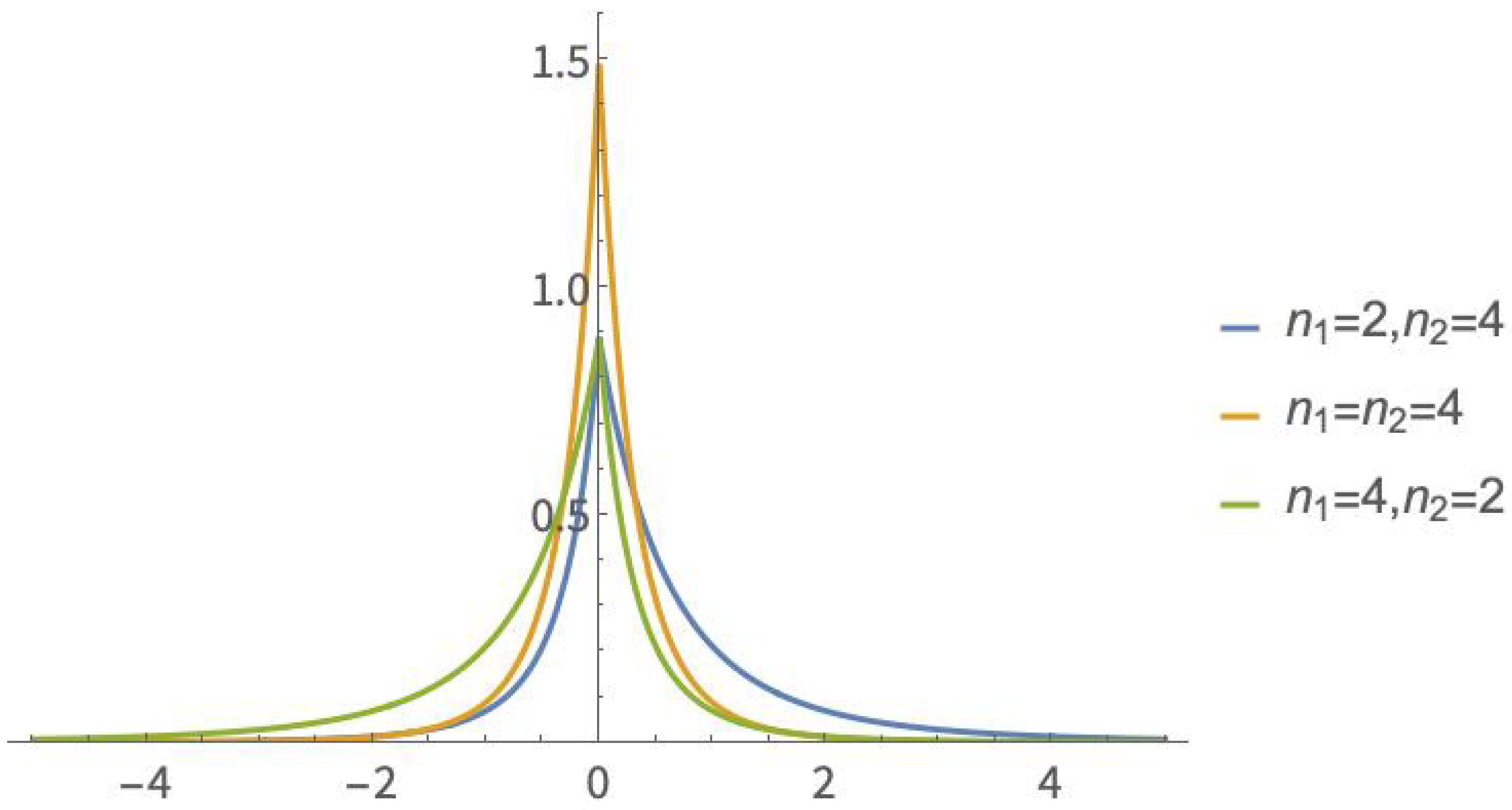
2.3. Joint Probability Density Function of $({\overline{X}}_n,S{S}_n)$

Let $\mathit{X}=(X_1,\dots ,X_{n+1})$, $n\ge 2$, be a random sample from the parent distribution X. From $({\overline{X}}_n,S{S}_n)$ and $X_{n+1}$ being independent, the joint probability density function of $({\overline{X}}_n,S{S}_n,X_{n+1})$ is

$$f_{({\overline{X}}_n,S{S}_n,X_{n+1})}(w,s,x)=f_{({\overline{X}}_n,S{S}_n)}(w,s)f_{X_{n+1}}\left(x\right)=f_{({\overline{X}}_n,S{S}_n)}(w,s)f_X\left(x\right).$$

On the other hand, as

$${\overline{X}}_{n+1}={\displaystyle \frac{n}{n+1}}{\overline{X}}_n+{\displaystyle \frac{X_{n+1}}{n+1}}\mathrm{and}S{S}_{n+1}=S{S}_n+{\displaystyle \frac{n}{n+1}}{({\overline{X}}_n-X_{n+1})}^2,$$

using the auxiliary random variable $Y={\overline{X}}_n-X_{n+1}$, the inverse transformation is

$${\overline{X}}_n={\overline{X}}_{n+1}+{\displaystyle \frac{Y}{n+1}},S{S}_n=S{S}_{n+1}-{\displaystyle \frac{n}{n+1}}{Y}^2\mathrm{and}{X}_{n+1}={\overline{X}}_{n+1}-{\displaystyle \frac{n}{n+1}}Y,$$

with $\left|J\right|=1$. Hence, the joint probability density function of $({\overline{X}}_{n+1},S{S}_{n+1},Y)$ is

$$f_{({\overline{X}}_{n+1},S{S}_{n+1},Y)}(w,s,y)=f_{({\overline{X}}_n,S{S}_n)}\left(w+{\displaystyle \frac{y}{n+1}},s-{\displaystyle \frac{n{y}^2}{n+1}}\right)f_X\left(w-{\displaystyle \frac{ny}{n+1}}\right),$$

and therefore, the joint probability density function of $({\overline{X}}_{n+1},S{S}_{n+1})$ is given by

$$f_{({\overline{X}}_{n+1},S{S}_{n+1})}(w,s)={\int }_{-\sqrt{{\displaystyle \frac{n+1}{n}}s}}^{\sqrt{{\displaystyle \frac{n+1}{n}}s}}{f}_{({\overline{X}}_n,S{S}_n)}\left(w+{\displaystyle \frac{y}{n+1}},s-{\displaystyle \frac{n{y}^2}{n+1}}\right)f_X\left(w-{\displaystyle \frac{ny}{n+1}}\right)\mathrm{d}y.$$

(8)

We emphasize that in integral (8), it is assumed that X has support $\mathbb{R}$, which we shall continue to assume for what follows, but if this is not the case, then the integration limits should be defined according to its support (see (6)).

In making the replacement $v={\displaystyle \frac{y}{\sqrt{\frac{n+1}{n}s}}}$ in (8), it follows that

$$f_{({\overline{X}}_{n+1},S{S}_{n+1})}(w,s)={\int }_{-1}^1\sqrt{\frac{n+1}{n}s}{f}_{({\overline{X}}_n,S{S}_n)}\left(w+v\sqrt{\frac{s}{n(n+1)}},s(1-v^2)\right)f_X\left(w-v\sqrt{\frac{ns}{n+1}}\right)\mathrm{d}v.$$

(9)

For example, if $n+1=3$, then in using Formulas (9) and (5),

$$\begin{array}{cc}\hfill f_{({\overline{X}}_3,S{S}_3)}(w,s)& ={\int }_{-1}^1\sqrt{{\displaystyle \frac{3}{2}}s}{f}_{({\overline{X}}_2,S{S}_2)}\left(w+v\sqrt{\frac{s}{6}},s(1-v^2)\right)f_X\left(w-v\sqrt{\frac{2}{3}s}\right)\mathrm{d}v\hfill \\ & =\sqrt{3}{\int }_{-1}^1{\displaystyle \frac{1}{\sqrt{1-v^2}}}{f}_X\left(w+\left(v+\sqrt{3(1-v^2)}\right)\sqrt{\frac{s}{6}}\right)\hfill \\ & \times f_X\left(w+\left(v-\sqrt{3(1-v^2)}\right)\sqrt{\frac{s}{6}}\right)f_X\left(w-2v\sqrt{\frac{s}{6}}\right)\mathrm{d}v\hfill \\ & =\sqrt{3}{\int }_{-1}^1{\displaystyle \frac{1}{\sqrt{1-v^2}}}{f}_X\left(w+\frac{v+\sqrt{3(1-v^2)}}{\sqrt{6}}\sqrt{s}\right)\hfill \\ & \times f_X\left(w+\frac{v-\sqrt{3(1-v^2)}}{\sqrt{6}}\sqrt{s}\right)f_X\left(w-\frac{2v}{\sqrt{6}}\sqrt{s}\right)\mathrm{d}v.\hfill \end{array}$$

(10)

Notice that the coefficients of $\sqrt{s}$ in the arguments of the functions in the last integrand in (10) satisfy the following two conditions:

$${\displaystyle \frac{v+\sqrt{3(1-v^2)}}{\sqrt{6}}}+{\displaystyle \frac{v-\sqrt{3(1-v^2)}}{\sqrt{6}}}-{\displaystyle \frac{2v}{\sqrt{6}}}=0$$

and

$${\left({\displaystyle \frac{v+\sqrt{3(1-v^2)}}{\sqrt{6}}}\right)}^2+{\left({\displaystyle \frac{v-\sqrt{3(1-v^2)}}{\sqrt{6}}}\right)}^2+{\left(-{\displaystyle \frac{2v}{\sqrt{6}}}\right)}^2=1.$$

2.4. The Gaussian Case

In applying (10), in particular, to the case $X\sim \mathrm{Gaussian}(0,\sigma )$, for $w\in \mathbb{R}$ and $s>0$,

$$\begin{array}{cc}\hfill f_{({\overline{X}}_3,S{S}_3)}(w,s)& =\sqrt{3}{\int }_{-1}^1{\displaystyle \frac{1}{\sqrt{1-v^2}}}{\displaystyle \frac{{\mathrm{e}}^{-\frac{s+3w^2}{2{\sigma }^2}}}{2\sqrt{2}{\pi }^{3/2}{\sigma }^3}}\mathrm{d}v\hfill \\ & =\sqrt{3}{\displaystyle \frac{{\mathrm{e}}^{-\frac{s+3w^2}{2{\sigma }^2}}}{2\sqrt{2}{\pi }^{3/2}{\sigma }^3}}{\int }_{-1}^1{\displaystyle \frac{1}{\sqrt{1-v^2}}}\mathrm{d}v\hfill \\ & ={\displaystyle \frac{1}{\sqrt{2\pi }\frac{\sigma }{\sqrt{3}}}}{\mathrm{e}}^{-{\displaystyle \frac{3w^2}{2{\sigma }^2}}}{\mathbb{I}}_{\mathbb{R}}\left(w\right){\displaystyle \frac{{\mathrm{e}}^{-\frac{s}{2{\sigma }^2}}}{2{\sigma }^2}}{\mathbb{I}}_{{\mathbb{R}}^{+}}\left(s\right)\hfill \\ & \approx f_X\left(w+\sqrt{\frac{s}{2}}\right)f_X\left(w\right)f_X\left(w-\sqrt{\frac{s}{2}}\right),\hfill \end{array}$$

(11)

where $\left\{{\displaystyle \frac{1}{\sqrt{2}}},0,-{\displaystyle \frac{1}{\sqrt{2}}}\right\}$ is a set of equidistant points such that their sum is 0 and the sum of their squares is 1.

As for the joint probability density function of $({\overline{X}}_4,S{S}_4)$, using the recurrence Formula (9), we obtain

$$f_{({\overline{X}}_4,S{S}_4)}(w,s)=\sqrt{{\displaystyle \frac{4s}{3}}}{\int }_{-1}^1{f}_{({\overline{X}}_3,S{S}_3)}\left(w+\sqrt{\frac{s}{12}}v,(1-v^2)s\right)f_X\left(w-\sqrt{\frac{3s}{4}}v\right)\mathrm{d}v,$$

(12)

and in view of what was established in (11), the joint probability density function (12) can be approximated using the product of $f_X$ computed at the points $w+{\alpha }_{i,4}\sqrt{s}$, $i=1,2,3,4$, i.e.,

$$f_{({\overline{X}}_4,S{S}_4)}(w,s)\approx K\sqrt{s}\prod _{i=1}^4{f}_X\left(w+{\alpha }_{i,4}\sqrt{s}\right),$$

(13)

with K as a norming constant, provided that ${\sum }_{i=1}^4{\alpha }_{i,4}=0$ and ${\sum }_{i=1}^4{\alpha }_{i,4}^2=1$.

In determining the points $w+{\alpha }_{i,4}\sqrt{s}$, since the set $A=\{{\alpha }_{1,4},{\alpha }_{2,4},{\alpha }_{3,4},{\alpha }_{3,4}\}$ is symmetric, for its elements to fulfill the first condition, they must satisfy $a_{1,4}=-a_{4,4}$ and $a_{2,4}=-a_{3,4}$. As the points are also equidistant, i.e., ${\alpha }_{i,4}-{\alpha }_{i-1,4}=r$, $i=2,3,4$, they form an arithmetic progression with common distance r, and thus, $A=\left\{{\displaystyle \frac{3r}{2}},{\displaystyle \frac{r}{2}},-{\displaystyle \frac{r}{2}},-{\displaystyle \frac{3r}{2}}\right\}$. In order to satisfy the second condition, we must also have $r^2={\displaystyle \frac{1}{5}}$, and hence,

$$A=\{{\alpha }_{1,4},{\alpha }_{2,4},{\alpha }_{3,4},{\alpha }_{3,4}\}=\left\{{\displaystyle \frac{3}{\sqrt{20}}},{\displaystyle \frac{1}{\sqrt{20}}},-{\displaystyle \frac{1}{\sqrt{20}}},-{\displaystyle \frac{3}{\sqrt{20}}}\right\}.$$

Therefore, from (13), and for $w\in \mathbb{R}$ and $s>0$, we obtain

$$f_{({\overline{X}}_4,S{S}_4)}(w,s)\approx {\mathrm{e}}^{-{\displaystyle \frac{4w^2}{2{\sigma }^2}}}\sqrt{s}{\mathrm{e}}^{-{\displaystyle \frac{s}{2{\sigma }^2}}}\propto f_{{\overline{X}}_4}\left(w\right)f_{S{S}_4}\left(s\right).$$

(14)

More generally, we have the following:

• If $n=2k+1$, then

  $$\left\{{\alpha }_{1,n},\dots ,{\alpha }_{n,n}\right\}=\left\{{\displaystyle \frac{n-1}{2}}r,\left({\displaystyle \frac{n-1}{2}}-1\right)r,\dots ,r,0,-r,\dots ,-\left({\displaystyle \frac{n-1}{2}}-1\right)r,-{\displaystyle \frac{n-1}{2}}r\right\},$$

  and from $2{\displaystyle \frac{\frac{n-1}{2}\frac{n+1}{2}n}{6}}{r}^2=1$, we obtain $r^2={\displaystyle \frac{12}{n(n^2-1)}}$.
• If $n=2k$, then

  $$\left\{{\alpha }_{1,n},\dots ,{\alpha }_{n,n}\right\}=\left\{{\displaystyle \frac{2n-1}{2}}r,{\displaystyle \frac{2n-3}{2}}r,\dots ,{\displaystyle \frac{r}{2}},-{\displaystyle \frac{r}{2}},\dots ,-{\displaystyle \frac{2n-3}{2}}r,-{\displaystyle \frac{2n-1}{2}}r\right\},$$

  and from $2{\sum }_{k=0}^{n/2}{\left({\displaystyle \frac{2k-1}{2}}\right)}^2{r}^2=1$, we obtain $r^2={\displaystyle \frac{12}{n(n^2-1)}}$.

It follows that ${\alpha }_{1,n}=\sqrt{{\displaystyle \frac{3(n-1)}{n(n+1)}}}$, and since ${\alpha }_{i,n}=\left({\displaystyle \frac{n-1}{2}}-i+1\right)r$, $i=1,\dots ,n$, we have

$${\alpha }_{i,n}=(n+1-2i)\sqrt{{\displaystyle \frac{3}{n(n^2-1)}}},i=1,\dots ,n.$$

In particular, ${\alpha }_{i,n-1}=(n-2i)\sqrt{{\displaystyle \frac{3}{(n-1)n(n-2)}}}$, and hence,

$$\sqrt{{\displaystyle \frac{n-2}{n+1}}}{\alpha }_{i,n-1}=(n-2i)\sqrt{{\displaystyle \frac{3}{n(n^2-1)}}}.$$

Therefore,

$${\alpha }_{i,n}-\sqrt{{\displaystyle \frac{n-2}{n+1}}}{\alpha }_{i,n-1}=\sqrt{{\displaystyle \frac{3}{n(n^2-1)}}}\left(={\displaystyle \frac{r}{2}}\right).$$

For example, for $n=2$ and $n=3$ we obtained the values

$$\begin{array}{cc}\hfill n=2:& {\alpha }_{1,2}={\displaystyle \frac{1}{\sqrt{2}}},{\alpha }_{2,2}=-{\displaystyle \frac{1}{\sqrt{2}}};\hfill \\ \hfill n=3:& {\alpha }_{1,3}={\displaystyle \frac{1}{\sqrt{2}}},{\alpha }_{2,3}=0,{\alpha }_{3,3}=-{\displaystyle \frac{1}{\sqrt{2}}}.\hfill \end{array}$$

As a recurrence formula,

$${\alpha }_{i,n}=\sqrt{{\displaystyle \frac{3}{n(n^2-1)}}}+\sqrt{{\displaystyle \frac{n-2}{n+1}}}{\alpha }_{i,n-1},i=1,\dots ,n-1,{\alpha }_{n,n}=-\sqrt{{\displaystyle \frac{3(n-1)}{n(n+1)}}}.$$

(15)

By expressing the multiplier $\sqrt{{\displaystyle \frac{n-2}{n+1}}}$ as $\sqrt{{\displaystyle \frac{n-2}{n+1}}}=\sqrt{1-{\xi }_n^2}$, we obtain ${\xi }_n=\sqrt{{\displaystyle \frac{3}{n+1}}}$.

3. Symmetry and Studentization

3.1. Symmetric Random Variables

There are useful results that enable the identification or characterization of symmetric random variables, such as the following:

(i)

If X and Y are independent random variables, then $W=XY$ has a characteristic function ${\phi }_W\left(t\right)=\mathbb{E}\left({\mathrm{e}}^{\mathrm{i}tXY}\right)={\int }_{-\infty }^{\infty }\mathbb{E}\left({\mathrm{e}}^{\mathrm{i}tXy}\right)\mathrm{d}{F}_Y\left(y\right)={\int }_{-\infty }^{\infty }{\phi }_X\left(ty\right)\mathrm{d}{F}_Y\left(y\right)$.

(ii)

If $X\sim \mathrm{Bernoulli}\left(\frac{1}{2}\right)$, then $B=2X-1$ has a probability mass function $\mathbb{P}(B=-1)=\mathbb{P}(B=1)=\frac{1}{2}$, and its characteristic function is ${\phi }_B\left(t\right)=\mathbb{E}\left({\mathrm{e}}^{\mathrm{i}tB}\right)={\displaystyle \frac{1}{2}}{\mathrm{e}}^{-\mathrm{i}t}+{\displaystyle \frac{1}{2}}{\mathrm{e}}^{\mathrm{i}t}=\cos t$.

(iii)

If X and B (B as defined in (ii)) are independent, the characteristic function of $W=BX$ is ${\phi }_W\left(t\right)={\int }_{-\infty }^{\infty }\cos \left(tx\right)\mathrm{d}{F}_X\left(x\right)$.

(iv)

A random variable is symmetric if and only if its characteristic function is ${\phi }_X\left(t\right)={\int }_{-\infty }^{\infty }\cos \left(tx\right)\mathrm{d}{F}_X\left(x\right)$.

From the above, a random variable X is symmetric if and only if $X\stackrel{d}{=}XB$, with X and B being independent. Therefore, if X and Y are independent random variables and X is symmetric, then $XY$ is also symmetric. In particular, if X is symmetric, then ${\overline{X}}_n$ is symmetric, which leads to $T_{n-1}$ being symmetric as well.

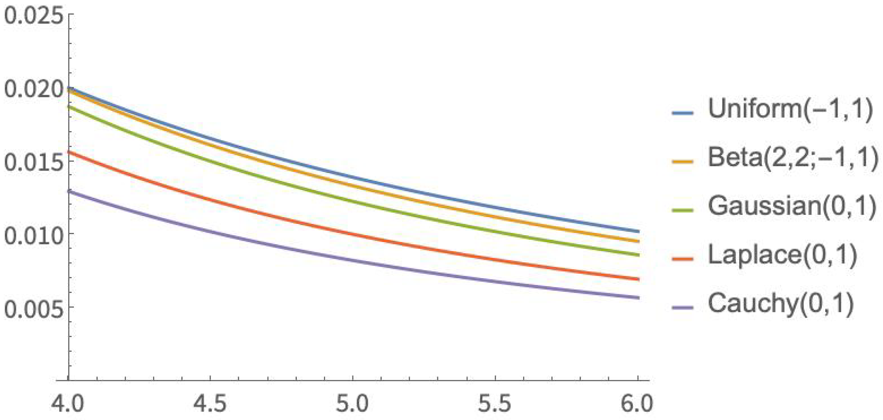
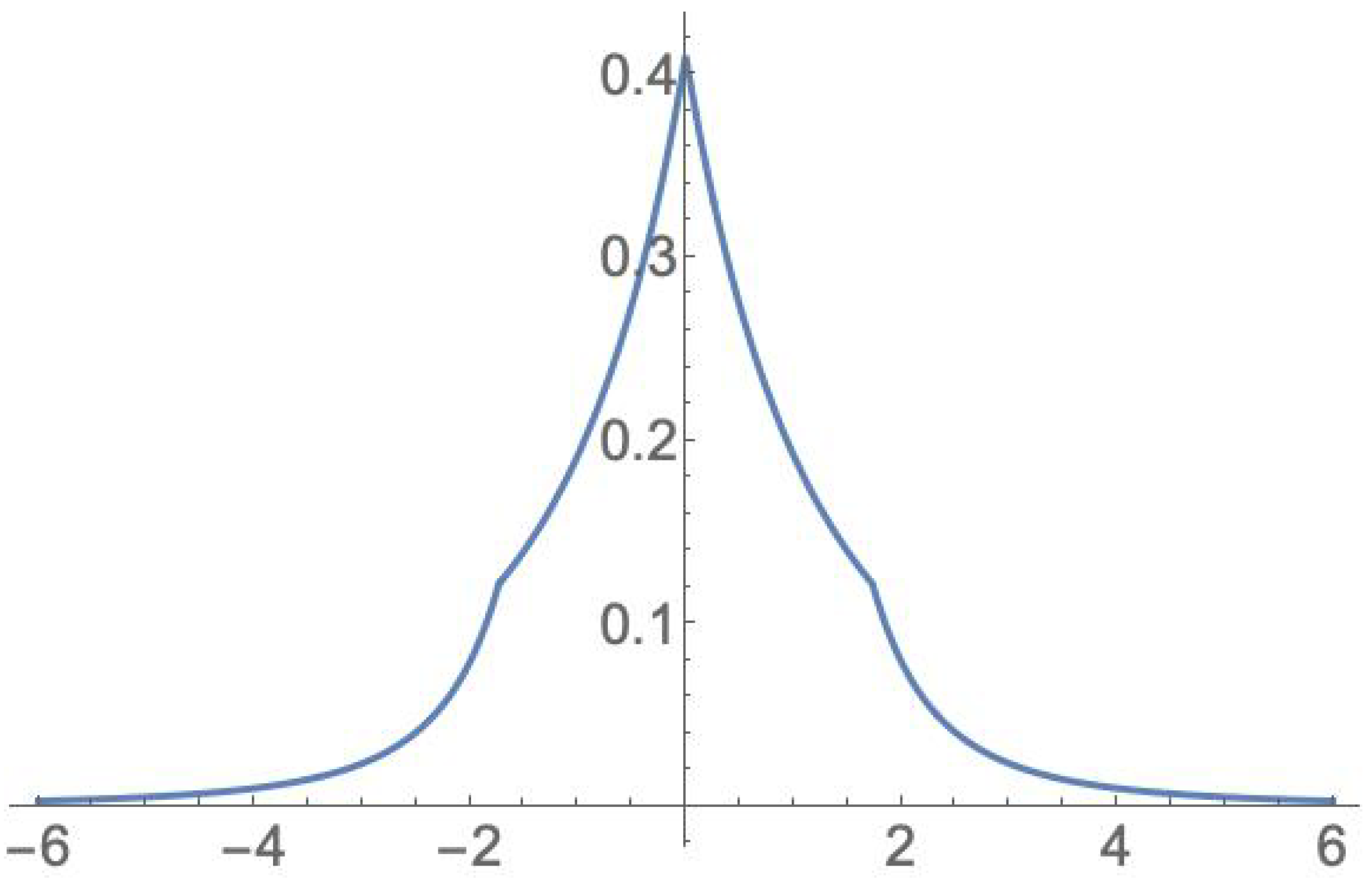
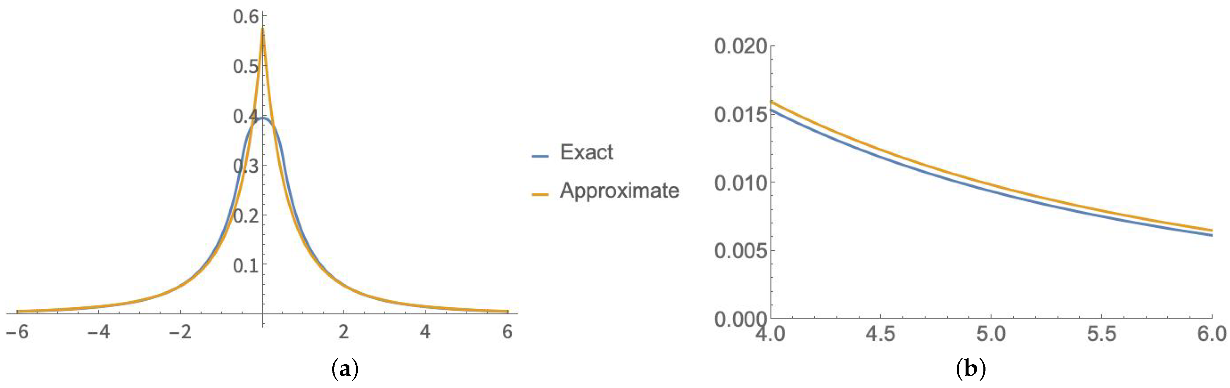
3.2. An Approximate Joint Probability Density Function of $({\overline{X}}_n,S{S}_n)$ with a Symmetric Parent Distribution

Using the Gaussian case as a guideline, for $n=3$, we assume that $f_X$ is a continuous and smooth probability density function of a symmetric random variable X, in the sense that there is a value ${\xi }_3\left(f_X\right)\in (-1,1)$ such that, from the mean value theorem, the integral in (10) can be computed as

$$\begin{array}{cc}\hfill f_{({\overline{X}}_3,S{S}_3)}(w,s)& ={\displaystyle \frac{1}{\sqrt{1-{\xi }_3^2}}}{f}_X\left(w+\frac{{\xi }_3+\sqrt{3(1-{\xi }_3^2)}}{\sqrt{6}}\sqrt{s}\right)\hfill \\ & \times f_X\left(w-\frac{{\xi }_3+\sqrt{3(1-{\xi }_3^2)}}{\sqrt{6}}\sqrt{s}\right)f_X\left(w-{\displaystyle \frac{2{\xi }_3}{\sqrt{6}}}\sqrt{s}\right)\hfill \\ & ={\displaystyle \frac{1}{\sqrt{1-{\xi }_3^2}}}\prod _{i=1}^3{f}_X\left(w+{\alpha }_{i,3}\left({\xi }_3\right)\sqrt{s}\right),\hfill \end{array}$$

(16)

where ${\alpha }_{1,3}\left({\xi }_3\right)={\displaystyle \frac{{\xi }_3+\sqrt{3(1-{\xi }_3^2)}}{\sqrt{6}}}$, ${\alpha }_{2,3}\left({\xi }_3\right)={\displaystyle \frac{-{\xi }_3-\sqrt{3(1-{\xi }_3^2)}}{\sqrt{6}}}$, and ${\alpha }_{2,3}\left({\xi }_3\right)=-{\displaystyle \frac{3{\xi }_3}{\sqrt{6}}}$, so that ${\sum }_{i=1}^3{\alpha }_{i,3}\left({\xi }_3\right)=0$ and ${\sum }_{i=1}^3{\alpha }_{i,3}^2\left({\xi }_3\right)=1$.

More generally, we investigate the consequences of a smoothness hypothesis, which is based on the Gaussian case.

Smoothness Hypothesis 1.

Let $X_1,X_2,\dots$ be independent replicas of a random variable X, with a smooth probability density function $f_X$ that allows the integral mean value theorem to be used. Therefore, for $\nu =2,\dots ,n$, there are values ${\xi }_{\nu }\left(f_X\right)\in (-1,1)$ and ${\alpha }_{i,\nu }\left({\xi }_{\nu }\right)$ of the form

$${\alpha }_{i,\nu }={\displaystyle \frac{{\xi }_{\nu }}{\sqrt{\nu (\nu -1)}}}+{\alpha }_{i,\nu -1}\sqrt{1-{\xi }_{\nu }^2},i=1,\dots ,\nu -1,\mathrm{and}{\alpha }_{\nu ,\nu }=-{\xi }_{\nu }\sqrt{{\displaystyle \frac{\nu -1}{\nu }}},$$

satisfying the conditions ${\sum }_{i=1}^{\nu }{\alpha }_{i,\nu }\left({\xi }_{\nu }\right)=0$ and ${\sum }_{i=1}^{\nu }{\alpha }_{i,\nu }^2\left({\xi }_{\nu }\right)=1$ such that the approximation

$$\begin{array}{cc}\hfill f_{({\overline{X}}_{\nu },S{S}_{\nu })}(w,s)& \approx K{s}^{(\nu -3)/2}\prod _{i=1}^{\nu }{f}_X(w+{\alpha }_{i,\nu }\sqrt{s}){\mathbb{I}}_{\mathcal{S}}(w,s),\hfill \end{array}$$

(17)

where K is a norming constant, is valid.

Then, the integral mean value theorem also holds for $f_{({\overline{X}}_{n+1},S{S}_{n+1})}$, i.e., there are values ${\xi }_{n+1}\left(f_X\right)\in (-1,1)$ and ${\alpha }_{i,n+1}\left({\xi }_{n+1}\right)$ such that the approximation

$$f_{({\overline{X}}_{n+1},S{S}_{n+1})}(w,s)\approx K{s}^{(n+1-3)/2}\prod _{i=1}^{n+1}{f}_X(w+{\alpha }_{i,n+1}\left({\xi }_{n+1}\right)\sqrt{s}){\mathbb{I}}_{\mathcal{S}}(w,s)$$

(18)

is also valid, with $({\overline{X}}_{n+1},S{S}_{n+1})$ having support $\mathcal{S}$ defined in (6), and ${\alpha }_{i,n+1}={\displaystyle \frac{{\xi }_{n+1}}{\sqrt{n(n+1)}}}+{\alpha }_{i,n}\sqrt{1-{\xi }_{n+1}^2}$, $i=1,\dots ,n$, and ${\alpha }_{n+1,n+1}=-{\xi }_{n+1}\sqrt{{\displaystyle \frac{n}{n+1}}}$.

If we further assume that X is a symmetric random variable, which implies that the points ${\alpha }_{1,n},\dots ,{\alpha }_{n,n}$ form an arithmetic progression with common distance $r_n=-{\displaystyle \frac{2\sqrt{3}}{\sqrt{n(n^2-1)}}}$ and ${\alpha }_{i,n}=-{\alpha }_{n+1-i,n}$, $i=1,\dots ,n$, then ${\xi }_n=\sqrt{{\displaystyle \frac{3}{n+1}}}$ and

$${\alpha }_{i,n}=(n+1-2i)\sqrt{{\displaystyle \frac{3}{n(n^2-1)}}},i=1,\dots ,n.$$

(19)

Equation (19) is easily obtained. In fact, if $n=2k+1$, then ${\alpha }_{1,n}=k\left|r_n\right|$. Moreover, the abcissas of the positive points ${\alpha }_{i,n}$ are $\left|r\right|,2\left|r\right|,\dots ,k\left|r\right|$, and since ${\sum }_{j=1}^k{\left(jr\right)}^2={\displaystyle \frac{1}{2}}$, this implies that $\left|r\right|=2\sqrt{{\displaystyle \frac{3}{n(n^2-1)}}}$. For $n=2k$, the results are similar, with the abcissas of the positive ${\alpha }_{i,n}$ now being ${\displaystyle \frac{\left|r\right|}{2}},{\displaystyle \frac{3\left|r\right|}{2}},\dots ,(k-{\displaystyle \frac{1}{2}})\left|r\right|$.

3.3. An Approximate Expression for the Probability Density Function of $T_{n-1}$ with a Smooth Symmetric Parent

Considering the transformation

$$T_{n-1}=\frac{\sqrt{n(n-1)}{\overline{X}}_n}{\sqrt{S{S}_n}}\mathrm{and}U=\sqrt{S{S}_n},$$

from which ${\overline{X}}_n=\frac{U{T}_{n-1}}{\sqrt{n(n-1)}}$ and $S{S}_n=U^2$, with $\left|J\right|={\displaystyle \frac{2U^2}{\sqrt{n(n-1)}}}$, we obtain

$$\begin{array}{cc}\hfill f_{(T_{n-1},U)}(t,u)& ={\displaystyle \frac{2u^2}{\sqrt{n(n-1)}}}{f}_{({\overline{X}}_n,S{S}_n)}\left(\frac{ut}{\sqrt{n(n-1)}},u^2\right),\hfill \end{array}$$

and therefore, for $t\in \mathbb{R}$, and X with support $\mathbb{R}$,

$$f_{T_{n-1}}\left(t\right)={\displaystyle \frac{2}{\sqrt{n(n-1)}}}{\int }_0^{\infty }{u}^2{f}_{({\overline{X}}_n,S{S}_n)}\left(\frac{ut}{\sqrt{n(n-1)}},u^2\right)\mathrm{d}u.$$

Using approximation (18), and denoting ${\alpha }_{i,n}\left({\xi }_n\right)={\alpha }_{i,n}$, it follows that

$$\begin{array}{c}\hfill f_{T_{n-1}}\left(t\right)\approx K{\int }_0^{\infty }{u}^{n-1}\prod _{i=1}^n{f}_X\left(\left(\frac{t}{\sqrt{n(n-1)}}+{\alpha }_{i,n}\right)u\right)\mathrm{d}u.\end{array}$$

(20)

For example, if $X\sim \mathrm{Gaussian}(0,1)$, then

$$\begin{array}{cc}\hfill f_{t_{n-1}}\left(t\right)& \approx K{\int }_0^{\infty }{u}^{n-1}\prod _{i=1}^n\exp \left\{-{\displaystyle \frac{1}{2}}{\left[\left({\displaystyle \frac{t}{\sqrt{n(n-1)}}}+{\alpha }_{i,n}\right)u\right]}^2\right\}\mathrm{d}u=\hfill \\ & =K{\int }_0^{\infty }{u}^{n-1}\exp \left[-{\displaystyle \frac{u^2}{2}}\left({\displaystyle \frac{t^2}{n-1}}+1\right)\right]\mathrm{d}u=K{\displaystyle \frac{1}{{\left(1+\frac{t^2}{n-1}\right)}^{n/2}}},\hfill \end{array}$$

as expected.

If $X\sim \mathrm{Laplace}(0,1)$, where $f_X\left(x\right)={\displaystyle \frac{1}{2}}{\mathrm{e}}^{-\left|x\right|}$, then

$$\begin{array}{cc}\hfill f_{T_{n-1}}\left(t\right)& \approx K{\int }_0^{\infty }{u}^{n-1}\prod _{i=1}^n\exp \left[-\left|\left({\displaystyle \frac{t}{\sqrt{n(n-1)}}}+{\alpha }_{i,n}\right)u\right|\right]\mathrm{d}u=\hfill \\ & =K{\int }_0^{\infty }{u}^{n-1}\exp \left(-u\sum _{i=1}^n\left|{\displaystyle \frac{t}{\sqrt{n(n-1)}}}+{\alpha }_{i,n}\right|\right)\mathrm{d}u,\hfill \end{array}$$

and therefore,

$$f_{T_{n-1}}\left(t\right)\approx K{\left(\sum _{i=1}^n\left|{\displaystyle \frac{t}{\sqrt{n(n-1)}}}+{\alpha }_{i,n}\right|\right)}^{-n}{\mathbb{I}}_{\mathbb{R}}\left(t\right).$$

In particular, if $n=3$,

$$f_{T_2}\left(t\right)\approx K{\left(\left|{\displaystyle \frac{t}{\sqrt{6}}}+{\displaystyle \frac{1}{\sqrt{2}}}\right|+{\displaystyle \frac{\left|t\right|}{\sqrt{6}}}+\left|{\displaystyle \frac{t}{\sqrt{6}}}-{\displaystyle \frac{1}{\sqrt{2}}}\right|\right)}^{-3}{\mathbb{I}}_{\mathbb{R}}\left(t\right).$$

(21)

Computing the norming constant so that the right-hand side of (21) is transformed into a probability density function, we obtain

$$f_{T_2}\left(t\right)\approx {\displaystyle \frac{9\sqrt{6}}{19}}{\left(\left|{\displaystyle \frac{t}{\sqrt{6}}}+{\displaystyle \frac{1}{\sqrt{2}}}\right|+{\displaystyle \frac{\left|t\right|}{\sqrt{6}}}+\left|{\displaystyle \frac{t}{\sqrt{6}}}-{\displaystyle \frac{1}{\sqrt{2}}}\right|\right)}^{-3}{\mathbb{I}}_{\mathbb{R}}\left(t\right).$$

In Figure 3, the approximate probability density function of $T_2$ with a $\mathrm{Laplace}(0,1)$ parent is represented.

Figure 3. Approximate probability density function of $T_2$ with a $\mathrm{Laplace}(0,1)$ parent.

For the non-Gaussian parent case, to assess how well approximation (20) works, we shall compare the exact probability density function of $T_2$ with a $\mathrm{Uniform}(-1,1)$ parent, given by Perlo [12], namely

$$f_{T_2}\left(t\right)=\left\{\begin{array}{cc}{\displaystyle \frac{\sqrt{3}\left(1-\frac{9t^2}{4-t^2}\right)}{2(4-t^2)\sqrt{1-t^2}}}+{\displaystyle \frac{3\sqrt{3}(t^2+2)}{{(4-t^2)}^{5/2}}}\mathrm{arctanh}\left(\sqrt{{\displaystyle \frac{1-{\mathrm{t}}^2}{4-{\mathrm{t}}^2}}}\right)\hfill & ,\left|t\right|\le {\displaystyle \frac{1}{2}}\hfill \\ {\displaystyle \frac{9\left(\frac{1}{\left|t\right|+1)}+\frac{3\left|t\right|}{t^2-4}\right)}{4\left(\right|t|+1)(4-t^2)}}+{\displaystyle \frac{3\sqrt{3}(t^2+2)}{{(t^2-4)}^{5/2}}}\arctan \left({\displaystyle \frac{\sqrt{t^2-4}}{\sqrt{3}(t+2)}}\right)\hfill & ,\left|t\right|>{\displaystyle \frac{1}{2}}\hfill \end{array}\right.,$$

(22)

with the approximation using (20).

As we are now dealing with a parent distribution with a limited support, the integration limits for (20) must be defined according to (6). In this case, the condition

$$-\sqrt{6}<ut<\sqrt{6}\wedge 0<u^2<2\min \left\{{\left({\displaystyle \frac{ut}{\sqrt{6}}}+1\right)}^2,{\left(1-{\displaystyle \frac{ut}{\sqrt{6}}}\right)}^2\right\}$$

must be satisfied, or equivalently,

$$-\sqrt{6}<ut<\sqrt{6}\wedge 0<u<\min \left\{\sqrt{2}\left({\displaystyle \frac{ut}{\sqrt{6}}}+1\right),\sqrt{2}\left(1-{\displaystyle \frac{ut}{\sqrt{6}}}\right)\right\}.$$

Hence, in denoting $a=\min \left\{\sqrt{2}\left({\displaystyle \frac{ut}{\sqrt{6}}}+1\right),\sqrt{2}\left(1-{\displaystyle \frac{ut}{\sqrt{6}}}\right)\right\}$, it follows that

$$f_{T_2}\left(t\right)\approx K{\int }_0^a{u}^2{\left({\displaystyle \frac{1}{2}}\right)}^3\mathrm{d}u\propto {\int }_0^a{u}^2\mathrm{d}u={\displaystyle \frac{2\sqrt{6}}{(\sqrt{3}+{\left|t\right|)}^3}}{\mathbb{I}}_{\mathbb{R}}\left(t\right).$$

(23)

Computing the norming constant K so that the function in the right-hand side of (23) becomes a probability density function, we obtain

$$f_{T_2}\left(t\right)\approx {\displaystyle \frac{3}{(\sqrt{3}+{\left|t\right|)}^3}}{\mathbb{I}}_{\mathbb{R}}\left(t\right).$$

(24)

In Figure 4, the exact and approximate probability density functions of $T_2$ with a $\mathrm{Uniform}(-1,1)$ parent, defined in (22) and (24), respectively, are plotted together. As can be observed, the approximation is not good in the central region of the distributions, but it is quite good in the tails of the distributions, which is where it actually matters because inferences are made using the tails of the distributions.

Figure 4. Probability density function of $T_2$ with a $\mathrm{Uniform}(-1,1)$ parent: (a) Exact and approximate densities. (b) Zoom in of right tails.

Observe that Hendriks et al. [11] analyzed why the Uniform parent is the least favorable one, as far as approximations are concerned, for the probability density function of $T_{n-1}$.

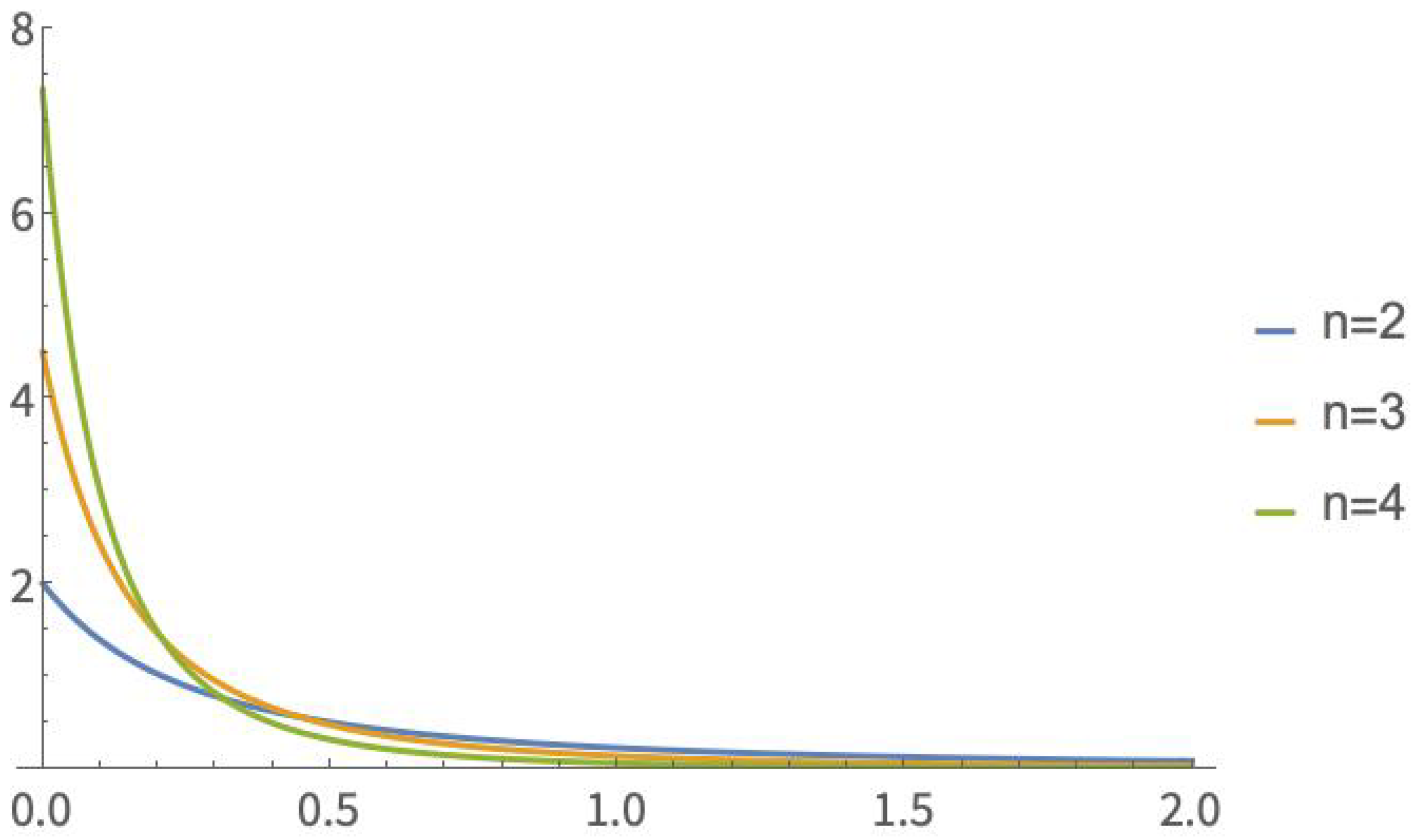
4. Externally Studentized Statistics Using Spacings of an Exponential Parent

4.1. External Studentization Using the Maximum Likelihood Scale Estimator

Let $\mathit{X}=\left(X_1,\dots ,X_n\right)$ be a random sample of size n from $X\sim Exponential(\lambda ,\delta )$, $\lambda \in \mathbb{R}$, $\delta >0$, i.e., with probability density function

$$f_X\left(x\right)={\displaystyle \frac{1}{\delta }}{\mathrm{e}}^{-{\displaystyle \frac{x-\lambda }{\delta }}}{\mathbb{I}}_{(\lambda ,\infty )}\left(x\right).$$

The maximum likelihood estimators $\widehat{\lambda }=X_{1:n}\sim \mathrm{Exponential}\left(\lambda ,{\displaystyle \frac{\delta }{n}}\right)$ and $\widehat{\delta }={\overline{X}}_n-X_{1:n}={\displaystyle \frac{1}{n}}{\sum }_{k=1}^n(X_{k:n}-X_{1:n})={\displaystyle \frac{1}{n}}{\sum }_{k=2}^n(n+1-k)(X_{k:n}-X_{k-1:n})\sim \mathrm{Gamma}\left(n-1,{\displaystyle \frac{\delta }{n}}\right)$ are independent due to the independence of the spacings $X_{k:n}-X_{k-1:n}\sim \mathrm{Exponential}\left(0,{\displaystyle \frac{\delta }{n+1-k}}\right)$, $k=1,\dots ,n$, with the usual convention $X_{0:n}=\lambda$.

Therefore, the externally Studentized statistic

$$T_{n-1}^{\ast }={\displaystyle \frac{X_{1:n}-\lambda }{{\overline{X}}_n-X_{1:n}}},$$

(25)

where $T_{n-1}^{\ast }\stackrel{d}{=}{\displaystyle \frac{Z_{1:n}}{{\overline{Z}}_n-Z_{1:n}}}$, with $(Z_1,\dots ,Z_n)$ being a random sample from $Z={\displaystyle \frac{X-\lambda }{\delta }}\sim \mathrm{Exponential}(0,1)$, has probability density function

$$\begin{array}{cc}\hfill f_{T_{n-1}^{\ast }}\left(t\right)& ={\int }_{-\infty }^{\infty }{f}_{Z_{1:n}}\left(tx\right)f_{{\overline{Z}}_n-Z_{1:n}}\left(x\right)\left|x\right|\mathrm{d}x\hfill \\ & ={\int }_0^{\infty }n{\mathrm{e}}^{-ntx}{\displaystyle \frac{n^{n-1}{x}^{n-2}{\mathrm{e}}^{-nx}}{\Gamma (n-1)}}x\mathrm{d}x\hfill \\ & ={\displaystyle \frac{n^n}{\Gamma (n-1)}}{\int }_0^{\infty }{x}^{n-1}{\mathrm{e}}^{-n(t+1)x}\mathrm{d}x\hfill \\ & ={\displaystyle \frac{n-1}{{(1+t)}^n}}{\mathbb{I}}_{(0,\infty )}\left(t\right),\hfill \end{array}$$

and hence, $T_{n-1}^{\ast }\sim \mathrm{Pareto}(n-1,0)$.

4.2. External Studentization Using the Sample Range as a Dispersion Estimator

Another externally Studentized statistic that can be used to make inferences on the location parameter $\lambda$ is

$${\tau }_{n-1}={\displaystyle \frac{X_{1:n}-\lambda }{X_{n:n}-X_{1:n}}}.$$

(26)

In noticing that ${\tau }_{n-1}\stackrel{d}{=}{\displaystyle \frac{Z_{1:n}}{Z_{n:n}-Z_{1:n}}}$ and considering that $Z_{n:n}-Z_{1:n}\stackrel{d}{=}{Z}_{n-1:n-1}$, the joint probability density function of $(Z_{1:n},Z_{n:n}-Z_{1:n})$ is

$$f_{(Z_{1:n},Z_{n:n}-Z_{1:n})}(x,y)=f_{Z_{1:n}}\left(x\right)f_{Z_{n:n}-Z_{1:n}}\left(y\right)=n{\mathrm{e}}^{-nx}(n-1){\left(1-{\mathrm{e}}^{-y}\right)}^{n-2}{\mathrm{e}}^{-y}{\mathbb{I}}_{{\mathbb{R}}^{+}\times {\mathbb{R}}^{+}}(x,y).$$

Using the transformation $S=Z_{1:n}$ and ${\tau }_{n-1}$, with $\left|J\right|={\displaystyle \frac{S}{{\tau }_{n-1}^2}}$, the joint probability density function of $(S,{\tau }_{n-1})$ is defined as

$$f_{(S,{\tau }_{n-1})}(s,t)=n(n-1){\mathrm{e}}^{-ns}{\mathrm{e}}^{-s/t}{(1-{\mathrm{e}}^{-s/t})}^{n-2}{\displaystyle \frac{s}{t^2}}{\mathbb{I}}_{{\mathbb{R}}^{+}\times {\mathbb{R}}^{+}}(s,t).$$

Therefore, for $t>0$,

$$\begin{array}{cc}\hfill f_{{\tau }_{n-1}}\left(t\right)& ={\displaystyle \frac{1}{t}}{\int }_0^{\infty }ns{\mathrm{e}}^{-ns}\left[(n-1){\mathrm{e}}^{-s/t}{(1-{\mathrm{e}}^{-s/t})}^{n-2}{\displaystyle \frac{1}{t}}\right]\mathrm{d}s\hfill \\ & =-{\displaystyle \frac{1}{t}}{\int }_0^{\infty }n(1-ns){\mathrm{e}}^{-ns}{(1-{\mathrm{e}}^{-s/t})}^{n-1}\mathrm{d}s\hfill \\ & =-{\displaystyle \frac{1}{t}}{\int }_0^{\infty }n{\mathrm{e}}^{-ns}{(1-{\mathrm{e}}^{-s/t})}^{n-1}\mathrm{d}s+{\displaystyle \frac{1}{t}}{\int }_0^{\infty }{n}^{2}s{\mathrm{e}}^{-ns}{(1-{\mathrm{e}}^{-s/t})}^{n-1}\mathrm{d}s.\hfill \end{array}$$

By making the replacement $u=1-{\mathrm{e}}^{-s/t}$ in the integrals, we obtain

$$\begin{array}{cc}\hfill f_{{\tau }_{n-1}}\left(t\right)& =-n{\int }_0^1{(1-u)}^{nt-1}{u}^{n-1}\mathrm{d}u-n^{2}t{\int }_0^1\ln (1-u){(1-u)}^{nt-1}{u}^{n-1}\mathrm{d}u\hfill \\ & =-n\left[B(n,nt)+nt{\displaystyle \frac{\partial B(n,nt)}{\partial \left(nt\right)}}\right].\hfill \end{array}$$

Since

$${\displaystyle \frac{\partial B(n,nt)}{\partial \left(nt\right)}}=B(n,nt)\left[\psi \left(nt\right)-\psi (n+nt)\right],$$

where $\psi \left(z\right)={\displaystyle \frac{\mathrm{d}}{\mathrm{d}z}}\ln z={\displaystyle \frac{{\Gamma }^{\prime }\left(z\right)}{\Gamma \left(z\right)}}$ is the digamma function, it follows that

$$f_{{\tau }_{n-1}}\left(t\right)=nB(n,nt)\left\{nt\left[\psi (n+nt)-\psi \left(nt\right)\right]-1\right\}{\mathbb{I}}_{(0,\infty )}\left(t\right).$$

(27)

Using the recurrence formula for the digamma function,

$$\psi (n+z)=\sum _{k=1}^n{\displaystyle \frac{1}{n-k+z}}+\psi \left(z\right),n\in \mathbb{N},$$

(cf. Abramowitz and Stegun [18]), the probability density function of ${\tau }_{n-1}$, given in (27), can be further simplified to

$$f_{{\tau }_{n-1}}\left(t\right)=nB(n,nt)\sum _{k=1}^{n-1}{\displaystyle \frac{nt}{n-k+nt}}{\mathbb{I}}_{(0,\infty )}\left(t\right).$$

In Table A1, in Appendix A, critical values of ${\tau }_{n-1}$ are displayed. The critical values were obtained using Mathematica v12. In Figure 5, the probability density function of ${\tau }_{n-1}$ is plotted for some values of n.

Figure 5. Probability density function of ${\tau }_{n-1}$.

For large values of n, an approximation can be used to obtain critical values of the statistic ${\tau }_{n-1}$. In recalling that $Z_{n:n}-Z_{1:n}\stackrel{d}{=}{Z}_{n-1:n-1}$, the limit distribution of the sequence of maxima ${(Z_{n-1:n-1}-\ln (n-1))}_{n\ge 2}$ is a standard Gumbel distribution, and therefore,

$$Z_{n:n}-Z_{1:n}-\ln (n-1)\underset{n\to \infty }{\overset{d}{\to }}V\sim \mathrm{Gumbel}(0,1).$$

Moreover, as $\underset{n\to \infty }{\lim }{\displaystyle \frac{\ln n}{\ln (n-1)}}=1$, in using the fact that ${\displaystyle \frac{Z_{n-1:n-1}}{\ln n}}\stackrel{P}{\to }1$ and $n{Z}_{1:n}\stackrel{d}{=}Z$, it follows from Slutsky’s theorem [19] that

$$n\ln n{\tau }_{n-1}\underset{n\to \infty }{\overset{d}{\to }}Z\sim \mathrm{Exponential}(0,1).$$

4.3. Internal Studentization Using Sums of Spacings

As the minimum $X_{1:n}$ and/or the maximum $X_{n:n}$ can be outliers, according to Hampel’s [20] breakdown point concept, the statistic ${\tau }_{n-1}$, defined in (26), can be unreliable. For an overview of robustness issues, see Rochetti [21], and in what concerns the duality of perspectives for extreme values/outliers, see Bhattacharya et al. [22]. For these reasons, it is more conservative to use instead the internally Studentized statistic

$${\tau }_{n-1;i,k}={\displaystyle \frac{{\overline{X}}_n-\lambda }{X_{k:n}-X_{i:n}}},$$

(28)

with $1<i<k<n$.

The sample mean ${\overline{X}}_n$ is a sufficient and complete estimator of $\lambda$, and the distribution of ${\tau }_{n-1;i,k}$ does not depend on the nuisance scale parameter $\delta$. Hence, from Basu’s [23] theorem, we conclude that ${\overline{X}}_n$ and ${\tau }_{n-1;i,k}$ are independent.

Noticing also that ${\tau }_{n-1;i,k}\stackrel{d}{=}{\displaystyle \frac{{\overline{Z}}_n}{Z_{k:n}-Z_{i:n}}}$, from the equality

$$Z_{k:n}-Z_{i:n}={\displaystyle \frac{{\overline{Z}}_n}{{\tau }_{n-1;i,k}}},$$

we must have $f_{Z_{k:n}-Z_{i:n}}=f_{{\displaystyle \frac{{\overline{Z}}_n}{{\tau }_{n-1;i,k}}}}$. Hence, from ${\overline{Z}}_n\sim \mathrm{Gamma}\left(n,\frac{1}{n}\right)$ and $Z_{k:n}-Z_{i:n}\stackrel{d}{=}{Z}_{k-i:n-i}$, we have for $x>0$,

$${\displaystyle \frac{\Gamma (n+1-i)}{\Gamma (k-i)\Gamma (n+1-k)}}{\mathrm{e}}^{-x(n+1-k)}{\left(1-{\mathrm{e}}^{-x}\right)}^{k-i-1}={\int }_0^{\infty }{f}_{{\overline{Z}}_n}\left(xt\right)f_{{\tau }_{n-1;i.k}}\left(t\right)t\mathrm{d}t,$$

i.e.,

$${\displaystyle \frac{\Gamma (n+1-i)}{\Gamma (k-i)\Gamma (n+1-k)}}{\mathrm{e}}^{-x(n+1-k)}{\left(1-{\mathrm{e}}^{-x}\right)}^{k-i-1}={\int }_0^{\infty }{\displaystyle \frac{n{\left(nxt\right)}^{n-1}{\mathrm{e}}^{-nxt}}{\Gamma \left(n\right)}}{f}_{{\tau }_{n-1;i.k}}\left(t\right)t\mathrm{d}t.$$

Thus, denoting $\mathcal{L}(f;x)$ the Laplace transform of function f at x, we obtain

$$\mathcal{L}(t^n{f}_{{\tau }_{n-1;i,k}}\left(t\right);x)={\displaystyle \frac{\Gamma \left(n\right)\Gamma (n+1-i)}{n\Gamma (k-i)\Gamma (n+1-k)}}{\displaystyle \frac{{\mathrm{e}}^{-x(n+1-k)/n}{(1-{\mathrm{e}}^{-x/n})}^{k-i-1}}{x^{n-1}}},$$

and in denoting ${\mathcal{L}}^{-1}(g;t)$ the inverse Laplace transform of function g at t, it follows that

$$f_{{\tau }_{n-1;i,k}}\left(t\right)={\displaystyle \frac{\Gamma \left(n\right)\Gamma (n+1-i)}{n\Gamma (k-i)\Gamma (n+1-k)}}{t}^{-n}{\mathcal{L}}^{-1}\left({\displaystyle \frac{{\mathrm{e}}^{-x(n+1-k)/n}{(1-{\mathrm{e}}^{-x/n})}^{k-i-1}}{x^{n-1}}};t\right).$$

(29)

For example, if $n=2$, $i=1$ and $k=2$,

$$f_{{\tau }_{1;1,2}}\left(t\right)={\displaystyle \frac{1}{2t^2}}{\mathcal{L}}^{-1}\left({\displaystyle \frac{{\mathrm{e}}^{-x/2}}{x}};t\right)={\displaystyle \frac{1}{2t^2}}{\mathbb{I}}_{({\displaystyle \frac{1}{2}},\infty )}\left(t\right),$$

i.e., ${\tau }_{1;1,2}\sim \mathrm{Pareto}(1,{\displaystyle \frac{1}{2}}).$

The most interesting scenario for (29) is when the integers n, i, and k satisfy the condition $n+1-k=k-i-1$, which occurs in the following cases:

• $n=3j-1$, $i=j-1$ and $k=2j$;
• $n=3j$, $i=j$ and $k=2j+1$;
• $n=3j+1$, $i=j+1$ and $k=2j+2$.

If this happens, then

$$f_{{\tau }_{n-1;i,k}}\left(t\right)={\displaystyle \frac{\Gamma \left(n\right)\Gamma (2j+1)}{n\Gamma \left(j\right)\Gamma (j+1)}}{\displaystyle \frac{1}{t^n}}{\mathcal{L}}^{-1}\left({\displaystyle \frac{1}{x^{k-2}}}{\left({\displaystyle \frac{{\mathrm{e}}^{-x/n}(1-{\mathrm{e}}^{-x/n})}{x}}\right)}^j;t\right).$$

Since

$${\mathcal{L}}^{-1}\left({\displaystyle \frac{1}{x^{k-2}}};t\right)={\displaystyle \frac{t^{k-3}}{\Gamma (k-2)}}\mathrm{and}{\mathcal{L}}^{-1}\left({\displaystyle \frac{{\mathrm{e}}^{-x/n}(1-{\mathrm{e}}^{-x/n})}{x}};t\right)={\mathbb{I}}_{({\displaystyle \frac{1}{n}},{\displaystyle \frac{2}{n}})}\left(t\right),$$

from the fact that the inverse Laplace transform of a product is the convolution of the inverse Laplace transforms of the factors, we obtain, for example, for $n=3$, $i=1$, and $k=3$,

$$f_{{\tau }_{2;1,3}}\left(t\right)=\left\{\begin{array}{cc}0& ,t<{\displaystyle \frac{1}{3}}\hfill \\ {\displaystyle \frac{4(t-\frac{1}{3})}{3t^3}}& ,{\displaystyle \frac{1}{3}}\le t<{\displaystyle \frac{2}{3}}\hfill \\ {\displaystyle \frac{4}{9t^3}}& ,t\ge {\displaystyle \frac{2}{3}}\hfill \end{array}\right.,$$

and for $n=4$, $i=2$, and $k=4$,

$$f_{{\tau }_{3;2,4}}\left(t\right)=\left\{\begin{array}{cc}0& ,t<{\displaystyle \frac{1}{4}}\hfill \\ {\displaystyle \frac{3{(4t-1)}^2}{32t^4}}& ,{\displaystyle \frac{1}{4}}\le t<{\displaystyle \frac{1}{2}}\hfill \\ {\displaystyle \frac{3(8t-3)}{32t^4}}& ,t\ge {\displaystyle \frac{1}{2}}\hfill \end{array}\right..$$

In Table A2, in Appendix A, critical values of ${\tau }_{n-1;i,k}$ are supplied for integers n, i, and k satisfying $n+1-k=k-i-1$. The critical values of ${\tau }_{n-1;i,k}$ were also obtained with Mathematica v12. The probability density functions of ${\tau }_{2;1,3}$ and ${\tau }_{3;2,4}$ are shown in Figure 6.

Figure 6. Probability density functions of ${\tau }_{2;1,3}$ and ${\tau }_{3;2,4}$.

4.4. Comparing the Locations of Two Exponential Populations with Equal Dispersions

For two exponential populations $X\sim \mathrm{Exponential}({\lambda }_1,{\delta }_1)$ and $Y\sim \mathrm{Exponential}({\lambda }_2,{\delta }_2)$, it may be of interest to make inferences on ${\lambda }_1-{\lambda }_2$. For this purpose, Theorem 1 can be helpful.

Theorem 1.

Let $X_1$ and $X_2$ be two independent random variables such that $X_1\sim \mathit{Exponential}({\lambda }_1,{\delta }_1)$ and $X_2\sim \mathit{Exponential}({\lambda }_2,{\delta }_2)$. Then, $X_1-X_2$ has an asymmetric Laplace distribution with probability density function

$$f_{X_1-X_2}\left(x\right)=\left\{\begin{array}{cc}{\displaystyle \frac{1}{{\delta }_1+{\delta }_2}}{\mathrm{e}}^{{\displaystyle \frac{x-({\lambda }_1-{\lambda }_2)}{{\delta }_2}}}\hfill & ,x\le {\lambda }_1-{\lambda }_2\hfill \\ {\displaystyle \frac{1}{{\delta }_1+{\delta }_2}}{\mathrm{e}}^{-{\displaystyle \frac{x-({\lambda }_1-{\lambda }_2)}{{\delta }_1}}}\hfill & ,x>{\lambda }_1-{\lambda }_2\hfill \end{array}\right..$$

Proof. 

Let $Y=(X_1-{\lambda }_1)-(X_2-{\lambda }_2)$. Since $X_1-{\lambda }_1\sim \mathrm{Exponential}(0,{\delta }_1)$ and $X_2-{\lambda }_2\sim \mathrm{Exponential}(0,{\delta }_2)$, for $y\le 0$,

$$\begin{array}{cc}\hfill f_Y\left(y\right)& ={\int }_{-y}^{\infty }{f}_{X_1-{\lambda }_1}(y+x)f_{X_2-{\lambda }_2}\left(x\right)\mathrm{d}x={\displaystyle \frac{1}{{\delta }_1{\delta }_2}}{\int }_{-y}^{\infty }{\mathrm{e}}^{-{\displaystyle \frac{y+x}{{\delta }_1}}}{\mathrm{e}}^{-{\displaystyle \frac{x}{{\delta }_2}}}\mathrm{d}x={\displaystyle \frac{1}{{\delta }_1+{\delta }_2}}{\mathrm{e}}^{{\displaystyle \frac{y}{{\delta }_2}}},\hfill \end{array}$$

and for $y>0$,

$$\begin{array}{cc}\hfill f_Y\left(y\right)& ={\int }_0^{\infty }{f}_{X_1-{\lambda }_1}(y+x)f_{X_2-{\lambda }_2}\left(x\right)\mathrm{d}x={\displaystyle \frac{1}{{\delta }_1{\delta }_2}}{\int }_0^{\infty }{\mathrm{e}}^{-{\displaystyle \frac{y+x}{{\delta }_1}}}{\mathrm{e}}^{-{\displaystyle \frac{x}{{\delta }_2}}}\mathrm{d}x={\displaystyle \frac{1}{{\delta }_1+{\delta }_2}}{\mathrm{e}}^{-{\displaystyle \frac{y}{{\delta }_1}}}.\hfill \end{array}$$

Hence, from $X_1-X_2\stackrel{d}{=}Y+({\lambda }_1-{\lambda }_2)$, it follows that

$$f_{X_1-X_2}\left(x\right)=f_Y(x-({\lambda }_1-{\lambda }_2))=\left\{\begin{array}{cc}{\displaystyle \frac{1}{{\delta }_1+{\delta }_2}}{\mathrm{e}}^{{\displaystyle \frac{x-({\lambda }_1-{\lambda }_2)}{{\delta }_2}}}\hfill & ,x\le {\lambda }_1-{\lambda }_2\hfill \\ {\displaystyle \frac{1}{{\delta }_1+{\delta }_2}}{\mathrm{e}}^{-{\displaystyle \frac{x-({\lambda }_1-{\lambda }_2)}{{\delta }_1}}}\hfill & ,x>{\lambda }_1-{\lambda }_2\hfill \end{array}\right..$$

□

If in Theorem 1 it is considered that ${\delta }_1={\delta }_2=\delta$, the symmetric Laplace distribution with location parameter ${\lambda }_1-{\lambda }_2\in \mathbb{R}$, and scale parameter $\delta >0$ is obtained. For more details on asymmetric Laplace random variables, see Brilhante and Kotz [24].

When dealing with two populations with equal dispersions, inferences on the difference between the locations of the two populations can be carried out using an externally Studentized statistic as described below.

Let $\mathit{X}=\left(X_1,\dots ,X_{n_1}\right)$ and $\mathit{Y}=\left(Y_1,\dots ,Y_{n_2}\right)$ be two independent random samples with parent distributions $X\sim \mathrm{Exponential}({\lambda }_1,\delta )$ and $Y\sim \mathrm{Exponential}({\lambda }_2,\delta )$, respectively. Considering that

$${\displaystyle \frac{X_{1:n_1}-{\lambda }_1}{\delta }}\sim \mathrm{Exponential}\left(0,\frac{1}{n_1}\right)\mathrm{and}{\displaystyle \frac{Y_{1:n_2}-{\lambda }_2}{\delta }}\sim \mathrm{Exponential}\left(0,\frac{1}{n_2}\right),$$

from Theorem 1,

$$U={\displaystyle \frac{X_{1:n_1}-Y_{1:n_2}-({\lambda }_1-{\lambda }_2)}{\delta }}$$

has probability density function

$$f_U\left(x\right)=\left\{\begin{array}{cc}{\displaystyle \frac{n_1{n}_2}{N}}{\mathrm{e}}^{n_{2}x}\hfill & ,x\le 0\hfill \\ {\displaystyle \frac{n_1{n}_2}{N}}{\mathrm{e}}^{-n_{1}x}\hfill & ,x>0\hfill \end{array}\right.,$$

with $N=n_1+n_2$.

On the other hand, as

$$n_1\left({\overline{X}}_{n_1}-X_{1:n_1}\right)=\sum _{k=2}^{n_1}(n_1+1-k)\left(X_{k:n_1}-X_{k-1:n_1}\right)\sim \mathrm{Gamma}(n_1-1,\delta ),$$

and, similarly, $n_2\left({\overline{Y}}_{n_2}-Y_{1:n_2}\right)\sim \mathrm{Gamma}(n_2-1,\delta )$, we have

$$V={\displaystyle \frac{\widehat{\delta }}{\delta }}={\displaystyle \frac{\left[n_1\left({\overline{X}}_{n_1}-X_{1:n_1}\right)+n_2\left({\overline{Y}}_{n_2}-Y_{1:n_2}\right)\right]/N}{\delta }}\sim \mathrm{Gamma}\left(N-2,\frac{1}{N}\right).$$

The independence of spacings in exponential populations ensures that U and V are independent, and therefore, the externally Studentized statistic $W_{n_1-1,n_2-1}={\displaystyle \frac{U}{V}}$, i.e.,

$$W_{n_1-1,n_2-1}={\displaystyle \frac{X_{1:n_1}-Y_{1:n_2}-({\lambda }_1-{\lambda }_2)}{\left[n_1({\overline{X}}_{n_1}-X_{1:n_1})+n_2({\overline{Y}}_{n_2}-Y_{1:n_2})\right]/N}},$$

can be used to make inferences on ${\lambda }_1-{\lambda }_2$.

As for the probability density function of $W_{n_1-1,n_2-1}$, for $w\le 0$,

$$\begin{array}{cc}\hfill f_{W_{n_1-1,n_2-1}}\left(w\right)& ={\int }_{-\infty }^{\infty }{f}_U\left(wx\right)f_V\left(x\right)\left|x\right|\mathrm{d}x\hfill \\ & ={\displaystyle \frac{n_1{n}_2{N}^{N-3}}{\Gamma (N-2)}}{\int }_0^{\infty }{x}^{N-2}{\mathrm{e}}^{-(N-n_{2}w)x}\mathrm{d}x\hfill \\ & ={\displaystyle \frac{n_1{n}_2(N-2)}{N^2{\left(1-\frac{n_2}{N}w\right)}^{N-1}}},\hfill \end{array}$$

and for $w>0$,

$$\begin{array}{cc}\hfill f_{W_{n_1-1,n_2-1}}\left(w\right)& ={\int }_{-\infty }^{\infty }{f}_U\left(wx\right)f_V\left(x\right)\left|x\right|\mathrm{d}x\hfill \\ & ={\displaystyle \frac{n_1{n}_2{N}^{N-3}}{\Gamma (N-2)}}{\int }_0^{\infty }{x}^{N-2}{\mathrm{e}}^{-(N+n_{1}w)x}\mathrm{d}x\hfill \\ & ={\displaystyle \frac{n_1{n}_2(N-2)}{N^2{\left(1+\frac{n_1}{N}w\right)}^{N-1}}}.\hfill \end{array}$$

Therefore,

$$f_{W_{n_1-1,n_2-1}}\left(w\right)=\left\{\begin{array}{cc}{\displaystyle \frac{n_1{n}_2(N-2)}{N^2{\left(1-\frac{n_2}{N}w\right)}^{N-1}}}\hfill & ,w\le 0\hfill \\ {\displaystyle \frac{n_1{n}_2(N-2)}{N^2{\left(1+\frac{n_1}{N}w\right)}^{N-1}}}\hfill & ,w>0\hfill \end{array}\right..$$

(30)

From (30), $\mathbb{P}(W\le 0)={\displaystyle \frac{n_1}{N}}$ and $\mathbb{P}(W>0)={\displaystyle \frac{n_2}{N}}=1-{\displaystyle \frac{n_1}{N}}$. Notice that ${\displaystyle \frac{n_1}{N}}$ is the proportion of observations in the combined sample that comes from the population X.

The critical value $W_{n_1-1,n_2-1;\alpha }$, $0<\alpha <1$, of $W_{n_1-1,n_2-1}$ is

$$W_{n_1-1,n_2-1;\alpha }=\left\{\begin{array}{cc}{\displaystyle \frac{N}{n_2}}\left[1-{\left({\displaystyle \frac{n_1}{N\alpha }}\right)}^{{\displaystyle \frac{1}{N-2}}}\right]\hfill & ,0<\alpha \le {\displaystyle \frac{n_1}{N}}\hfill \\ {\displaystyle \frac{N}{n_1}}\left[{\left({\displaystyle \frac{n_2}{N(1-\alpha )}}\right)}^{{\displaystyle \frac{1}{N-2}}}-1\right]\hfill & ,{\displaystyle \frac{n_1}{N}}<\alpha <1\hfill \end{array}\right..$$

If a balanced design is considered instead, i.e., $n_1=n_2=n$ in (30), denoting, for simplicity, $W_{n-1,n-1}=W_{n-1}$, then

$$f_{W_{n-1}}\left(w\right)={\displaystyle \frac{n-1}{2{\left(1+\frac{\left|w\right|}{2}\right)}^{2n-1}}}{\mathbb{I}}_{\mathbb{R}}\left(w\right).$$

(31)

The $(1-\alpha )$-th critical value of $W_{n-1}$ is $W_{n-1;1-\alpha }=2\left({\displaystyle \frac{1}{{\left(2\alpha \right)}^{1/2(n-1)}}}-1\right)$, $\alpha <0.5$. (The distribution of $W_{n-1}$ is symmetric around zero.)

In Figure 7, the probability density function of $W_{n_1,n_2}$ is plotted for some values of $n_1$ and $n_2$.

Figure 7. Probability density function of $W_{n_1-1,n_2-1}$.

Observe that if the two populations have unequal dispersions, i.e., ${\delta }_1\ne {\delta }_2$, the distribution of $W_{n_1-1,n_2-1}$ depends on the nuisance scale parameters ${\delta }_1$ and ${\delta }_2$, and so, it cannot be used to make inferences on ${\lambda }_1-{\lambda }_2$, unless a Satterthwaite [15] approximation is considered (for more details, see Section 4.6).

4.5. Analysis of Spacings (ANOSp) for Testing Homogeneity of $k>2$ Locations of Exponential Populations with Equal Dispersions

Let ${\mathit{X}}_{\mathbf{1}}=\left(X_{11},\dots ,X_{1n_1}\right),\dots ,{\mathit{X}}_{\mathit{k}}=\left(X_{k1},\dots ,X_{k{n}_k}\right)$ be $k>2$ independent random samples, with $X_{ij}\sim \mathrm{Exponential}({\lambda }_i,{\delta }_i)$, $i=1,\dots ,k$, $j=1,\dots ,n_i$. For what follows, we shall use the notations ${\overline{X}}_i$ for the sample mean and $X_{j:n_i}^{\left(i\right)}$ for the j-th ascending order statistic, $j=1,\dots ,n_i$, of the i-th random sample, $i=1,\dots ,k$. We shall also use the notations $\overline{X}={\displaystyle \frac{1}{N}}{\sum }_{i=1}^k{\sum }_{j=1}^{n_i}{X}_{ij}$ and $X_{1:N}={\min }_{\begin{array}{c}1\le i\le k\\ 1\le j\le n_i\end{array}}{X}_{ij}=\underset{1\le i\le k}{\min }{X}_{1:n_i}^{\left(i\right)}$, with $N=n_1+\cdots +n_k$ denoting the size of the combined samples.

The maximum likelihood estimators of the location and scale parameters of the individual populations are

$${\widehat{\lambda }}_i=X_{1:n_i}^{\left(i\right)}\sim \mathrm{Exponential}\left({\lambda }_i,\frac{{\delta }_i}{n_i}\right)\mathrm{and}{\widehat{\delta }}_i={\overline{X}}_i-X_{1:n_i}^{\left(i\right)}\sim \mathrm{Gamma}\left(n_i-1,\frac{{\delta }_i}{n_i}\right),$$

$i=1,\dots ,k$. Our interest lies in testing the homogeneity of locations of the populations, i.e., testing

$$H_0:{\lambda }_1=\cdots ={\lambda }_k(=\lambda )\mathrm{vs}.H_A:{\lambda }_i\ne {\lambda }_j,\mathrm{for}\mathrm{some}i,j\in \{1,,\dots ,k\},i\ne j.$$

For the time being, we shall assume that the populations have equal dispersions, i.e., ${\delta }_1=\dots ={\delta }_k=\delta$.

In this setting, a parallelism with a one-way ANOVA scheme can be made, since the Total Sum of Spacings (TSSp) can be split into a Between Sum of Spacings (BSSp) and a Within Sum of Spacings (WSSp) as follows:

$$\begin{array}{cc}\hfill \mathrm{TSSp}& =\sum _{i=1}^k\sum _{j=1}^{n_i}\left(X_{ij}-X_{1:N}\right)\hfill \\ & =\sum _{i=1}^k\sum _{j=1}^{n_i}\left[\left(X_{ij}-X_{1:n_i}^{\left(i\right)}\right)+\left(X_{1:n_i}^{\left(i\right)}-X_{1:N}\right)\right]\hfill \\ & =\sum _{i=1}^k{n}_i\left(X_{1:n_i}^{\left(i\right)}-X_{1:N}\right)+\sum _{i=1}^k\sum _{j=1}^{n_i}\left(X_{ij}-X_{1:n_i}^{\left(i\right)}\right)\hfill \\ & =\mathrm{BSSp}+\mathrm{WSSp}.\hfill \end{array}$$

In noticing that

$$\begin{array}{cc}\hfill \mathrm{WSSp}& =\sum _{i=1}^k\sum _{j=2}^{n_i}\left(X_{j:n_i}^{\left(i\right)}-X_{1:n_i}^{\left(i\right)}\right)=\sum _{i=1}^k\sum _{j=2}^{n_i}(n_i+1-j)\left(X_{j:n_i}^{\left(i\right)}-X_{j-1:n_i}^{\left(i\right)}\right)\sim \mathrm{Gamma}(N-k,\delta ),\hfill \end{array}$$

the statistic $\frac{\mathrm{WSSp}}{N-k}$ is an unbiased estimator of $\delta$, regardless of the validity of $H_0$.

On the other hand, under $H_0$, the random variables $Y_i=n_i{X}_{1:n_i}^{\left(i\right)}\sim \mathrm{Exponential}(\lambda ,\delta )$, $i=1,\dots ,k$, are independent. Thus, from

$$\mathrm{BSSp}=\sum _{i=1}^k{n}_i\left(X_{1:n}^{\left(i\right)}-X_{1:N}\right)=\sum _{i=1}^k{n}_i{X}_{1:n_i}^{\left(i\right)}-N{X}_{1:N}$$

and $N{X}_{1:N}\stackrel{d}{=}k{Y}_{1:k}$, with $Y_{1:k}=\min \{Y_1,\dots ,Y_k\}$, it follows that

$$\mathrm{BSSp}\stackrel{d}{=}\sum _{i=1}^k{Y}_i-k{Y}_{1:k}=k\left({\overline{Y}}_k-Y_{1:k}\right)\sim \mathrm{Gamma}\left(k-1,\delta \right).$$

Thus, under $H_0$, the statistic ${\displaystyle \frac{\mathrm{BSSp}}{k-1}}$ is an unbiased estimator of $\delta$.

From the above, and under $H_0$, the F-statistic

$$F={\displaystyle \frac{\mathrm{MBSSp}}{\mathrm{MWSSp}}}={\displaystyle \frac{\frac{\mathrm{BSSp}}{k-1}}{\frac{\mathrm{WSSp}}{N-k}}}={\displaystyle \frac{\frac{\mathrm{BSSp}/\left(2\delta \right)}{2(k-1)}}{\frac{\mathrm{WSSp}/\left(2\delta \right)}{2(N-k)}}}\sim F_{2(k-1),2(N-k)}$$

(32)

can detect gross departures from the null hypothesis. Notice that the independence of spacings in exponential populations guarantees the independence of BSSp and WSSp.

An ANOSp table, similar to a one-way ANOVA table, can be shown in this context (see Table 1).

Table 1. ANOSp table.

Sum of Spacings	df	Mean of Sum of Spacings	F-Statistic
$\mathrm{BSSp}={\displaystyle \sum _{i=1}^k}{n}_i\left(X_{1:n_i}^{\left(i\right)}-X_{1:N}\right)$	$2(k-1)$	$\mathrm{MBSSp}={\displaystyle \frac{\mathrm{BSSp}}{2(k-1)}}$	$F={\displaystyle \frac{\mathrm{MBSSp}}{\mathrm{MWSSp}}}={\displaystyle \frac{\frac{\mathrm{BSSp}}{k-1}}{\frac{\mathrm{WSSp}}{N-k}}}$
$\mathrm{WSSp}={\displaystyle \sum _{i=1}^k\sum _{j=1}^{n_i}}\left(X_{ij}-X_{1:n_i}^{\left(i\right)}\right)$	$2(N-k)$	$\mathrm{MWSSp}={\displaystyle \frac{\mathrm{WSSp}}{2(N-k)}}$

4.6. Analysis of Spacings (ANOSp) for Testing Homogeneity of $k>2$ Locations of Exponential Populations with Unequal Dispersions

If the exponential populations have unequal dispersions, the statistic defined in (32) is useless, because its distribution depends now on the nuisance scale parameters of the individual populations. However, a Satterthwaite approximation can be considered to eliminate its distribution’s dependence on those nuisance parameters.

Satterthwaite [15] showed that if $Y_1,\dots ,Y_n$ are independent random variables such that $Y_i\sim {\chi }_{{\nu }_i}^2$, $i=1,\dots ,n$, the linear combination ${\sum }_{i=1}^n{a}_i{Y}_i$, with $a_i\in \mathbb{R}$, $i=1,\dots ,n$, can be approximated using ${\displaystyle \frac{Y}{\nu }}$, where $Y\sim {\chi }_v^2$, i.e., ${\sum }_{i=1}^n{a}_i{Y}_i\approx {\displaystyle \frac{Y}{\nu }}$, where the degree of freedom $\nu$ is estimated using the estimator

$$\tilde{\nu }={\displaystyle \frac{{\left({\sum }_{i=1}^n{a}_i{Y}_i\right)}^2}{{\sum }_{i=1}^n\frac{a_i^2}{{\nu }_i}{Y}_i^2}}.$$

(33)

Since under $H_0$, the distribution of MBSSp does not depend on $\lambda$, we shall assume, without loss of generality, that $\lambda =0$. We shall also assume that from $X_{1:N}=\underset{1\le i\le k}{\min }{X}_{1:n_i}^{\left(i\right)}$, in particular, $X_{1:N}=X_{1:n_1}^{\left(1\right)}$, and therefore,

$$\begin{array}{cc}\hfill \mathrm{MBSSp}& ={\displaystyle \frac{1}{k-1}}\sum _{i=1}^k{n}_i\left(X_{1:n_i}^{\left(i\right)}-X_{1:N}\right)\hfill \\ & ={\displaystyle \frac{1}{k-1}}\sum _{i=1}^k{n}_i\left(X_{1:n_i}^{\left(i\right)}-X_{1:n_1}^{\left(1\right)}\right)\hfill \\ & ={\displaystyle \frac{n_1-N}{k-1}}{X}_{1:n_1}^{\left(1\right)}+\sum _{i=2}^k{\displaystyle \frac{n_i}{k-1}}{X}_{1:n_i}^{\left(i\right)}\hfill \\ & ={\displaystyle \frac{n_1-N}{k-1}}{\widehat{\lambda }}_1+\sum _{i=2}^k{\displaystyle \frac{n_i}{k-1}}{\widehat{\lambda }}_i,\hfill \end{array}$$

which can be expressed as

$$\mathrm{MBSSp}={\displaystyle \frac{{\delta }_1(n_1-N)}{2n_1(k-1)}}{Y}_1+\sum _{i=2}^k{\displaystyle \frac{{\delta }_i}{2(k-1)}}{Y}_i\approx {\displaystyle \frac{U}{{\nu }_1}},$$

with $Y_i={\displaystyle \frac{2n_i}{{\delta }_i}}{\widehat{\lambda }}_i\sim {\chi }_2^2$, $i=1,\dots ,k$, and $U\sim {\chi }_{{\nu }_1}^2$. In using $a_1={\displaystyle \frac{{\delta }_1(n_1-N)}{2n_1(k-1)}}$ and $a_i={\displaystyle \frac{{\delta }_i}{2(k-1)}}$, $i=2,\dots ,k$, in Formula (33), the parameter ${\nu }_1$ is estimated by

$${\tilde{\nu }}_1={\displaystyle \frac{2\left({\sum }_{i=1}^k{n}_i{\widehat{\lambda }}_i-N{\widehat{\lambda }}_1\right)}{{(n_1-N)}^2{\widehat{\lambda }}_1^2+{\sum }_{i=2}^k{n}_i^2{\widehat{\lambda }}_i^2}}.$$

(34)

On the other hand, noticing that

$$\begin{array}{cc}\hfill \mathrm{MWSSp}& ={\displaystyle \frac{1}{N-k}}\sum _{i=1}^k\sum _{j=1}^{n_i}\left(X_{ij}-X_{1:n_i}^{\left(i\right)}\right)\hfill \\ & ={\displaystyle \frac{1}{N-k}}\sum _{i=1}^k{n}_i\left({\overline{X}}_i-X_{1:n_i}^{\left(i\right)}\right)\hfill \\ & =\sum _{i=1}^k{\displaystyle \frac{n_i}{N-k}}{\widehat{\delta }}_i,\hfill \end{array}$$

with ${\widehat{\delta }}_i\sim \mathrm{Gamma}(n_i-1,{\delta }_i)$, $i=1,\dots ,k$, and then considering $Y_i={\displaystyle \frac{2}{{\delta }_i}}{\widehat{\delta }}_i\sim {\chi }_{2(n_i-1)}^2$, $i=1,\dots ,k$, we have

$$\mathrm{MWSSp}=\sum _{i=1}^k{\displaystyle \frac{n_i{\delta }_i}{2(N-K)}}{Y}_i\approx {\displaystyle \frac{V}{{\nu }_2}},$$

with $V\sim {\chi }_{{\nu }_2}^2$. In using $a_i={\displaystyle \frac{n_i{\delta }_i}{2(N-K)}}$, $i=1,\dots ,n$, in Formula (33), the parameter ${\nu }_2$ is estimated by

$${\tilde{\nu }}_2={\displaystyle \frac{2{\left({\sum }_{i=1}^k{n}_i{\widehat{\delta }}_i\right)}^2}{{\sum }_{i=1}^k\frac{n_i^2}{n_i-1}{\widehat{\delta }}_i^2}}.$$

(35)

Consequently, under $H_0$, U and V are independent, and therefore,

$$F={\displaystyle \frac{\mathrm{MBSSp}}{\mathrm{MWSSp}}}\approx {\displaystyle \frac{U/{\nu }_1}{V/{\nu }_2}}\sim F_{{\nu }_1,{\nu }_2},$$

where the degrees of freedom ${\nu }_1$ and ${\nu }_2$ of the F-statistic are estimated using (34) and (35), respectively.

5. Conclusions

The exact distribution of externally Studentized statistics in Gaussian samples and in exponential samples are readily obtained. The members of the location-scale exponential family with a pair of sufficient statistics for the parameters are as follows:

• $X\sim \mathrm{Gaussian}(\mu ,\sigma )$, when the support is the real line;
• $Y\sim \mathrm{Exponential}(\lambda ,\delta )$, when the support is the half-line $(\lambda ,\infty )$ (or the reverted exponential when the support is $(-\infty ,\lambda )$, in which case the pair of sufficient statistics is $\left(Y_{n:n},{\sum }_{k=1}^n{Y}_k\right)$, and the maximum likelihood estimators of the parameters are $\widehat{\lambda }=Y_{n:n}$ and $\widehat{\delta }=Y_{n:n}-{\overline{Y}}_n$);
• $W\sim \mathrm{Uniform}(\lambda ,\lambda +\delta )$ when the support is a segment, in which case the pair of sufficient statistics is $(W_{1:n},W_{n:n})$ and the maximum likelihood estimators of the parameters are $\widehat{\lambda }=W_{1:n}$ and $\widehat{\delta }=W_{n:n}-W_{1:n}$.

While for Gaussian samples and for exponential samples, the probability density functions of externally Studentized statistics are easily obtained, in the case of uniform samples, this is not possible. However, as uniform random variables are symmetric by default, the approximation under the smoothness hypothesis 1 holds, although it is known from Hendriks [11] that this is the worst framework to consider. Alternatively, as uniform samples can be logarithmically transformed into exponential data, inferences on the location parameter(s) can be dealt with using the results of Section 4.

On the other hand, it is, in general, impossible to obtain exact results for internally Studentized statistics. As Hotelling [25], Efron [10], and Lehman [26] have shown, symmetry for the parent distribution is a useful property for Studentizations. The investigation of the approximation resulting from the smoothness hypothesis (17) for symmetric parents, inspired by the Gaussian case, shows that even in the worst $\mathrm{Uniform}(-1,1)$ case, which was identified by Hendriks et al. [11] as such, the approximation in the tails is quite good, and therefore, it is usable for inferences on the location parameter.

With regard to asymmetric exponential parent distributions, from the independence of spacings, exact results either for one sample inferences on the location parameter or for the comparison of $k\ge 2$ location parameters assuming equal dispersions are straightforward. An approximate solution for the unequal dispersions case, inspired by Satterthwaite’s [15] treatment for comparing means in heteroscedastic Gaussian parents, has been presented.

References

- Student. The probable error of a mean. Biometrika 1908, 6, 1–25. [Google Scholar] [CrossRef]
- Geary, R.C. Distribution of Student’s ratio for nonnormal samples. Suppl. J. R. Stat. Soc. 1936, 3, 178–184. [Google Scholar] [CrossRef]
- Darmois, G. Analyse générale des liaisons stochastiques: Étude particuière de l’analyse factorielle lineéaire. Rev. L’Institut Int. Stat./Rev. Int. Stat. Inst. 1953, 21, 2–8. [Google Scholar] [CrossRef]
- Skitovich, V.P. Linear forms of independent random variables and the normal distribution law. Izv. Akad. Nauk SSSR Ser. Mat. 1954, 18, 185–200, (English Translation Sel. Transl. Math. Stat. Probab. 1962, 2, 211–218). [Google Scholar]
- Koopman, B.O. On distributions admitting a sufficient statistic. Trans. Am. Math. Soc. 1936, 39, 399–409. [Google Scholar] [CrossRef]
- Darmois, G. Sur les lois de probabilités à estimation exhaustive. Comptes Rendus L’Acad. Sci. Paris 1935, 200, 1265–1266. [Google Scholar]
- Pitman, E. Sufficient statistics and intrinsic accuracy. Math. Proc. Camb. Philos. Soc. 1936, 32, 567–579. [Google Scholar] [CrossRef]
- Logan, B.F.; Mallows, C.L.; Rice, S.O.; Shepp, L.A. Limit distributions of self-normalized sums. Ann. Probab. 1973, 1, 788–809. [Google Scholar] [CrossRef]
- Peña, V.H.D.L.; Lai, T.L.; Shao, Q.M. Self-Normalized Processes. Limit Theory and Statistical Applications; Springer: Berlin/Heidelberg, Germany, 2009. [Google Scholar]
- Efron, B. Student’s t-test under symmetry conditions. J. Am. Stat. Assoc. 1969, 64, 1278–1302. [Google Scholar] [CrossRef]
- Hendriks, H.W.M.; Ijzerman-Boon, P.C.; Klaassen, C.A.J. Student’s t-statistic under unimodal densities. Austrian J. Stat. 2006, 35, 131–141. [Google Scholar] [CrossRef]
- Perlo, V. On the distribution of Student’s ratio for samples of three drawn from the rectangular distribution. Biometrika 1933, 25, 203–204. [Google Scholar] [CrossRef]
- Pexider, J.V. Notiz über Funkcionaltheoreme. Monatsh. Math. Phys. 1903, 14, 293–301. [Google Scholar] [CrossRef]
- David, H.A. Order Statistics; Wiley: New York, NY, USA, 1981. [Google Scholar]
- Satterthwaite, F.E. An approximate distribution of estimates of variance components. Biom. Bull. 1946, 2, 110–114. [Google Scholar] [CrossRef]
- van Zwet, W. Convex Transformations of Random Variables, 7th ed.; Mathematical Centre: Amsterdam, The Netherlands, 1964. [Google Scholar]
- van Zwet, W. Convex transformations: A new approach to skewness and kurtosis. Statist. Neerl. 1964, 18, 433–441. [Google Scholar] [CrossRef]
- Abramowitz, M.; Stegun, I.A. Handbook of Mathematical Functions: With Formulas, Graphs, and Mathematical Tables, 8th ed.; Dover: New York, NY, USA, 1972. [Google Scholar]
- Slutsky, E. Über stochastische Asymptoten und Grenzwerte. Metron 1964, 5, 3–89. [Google Scholar]
- Hampel, F.R. Contributions to the Theory of Robust Estimation. Ph.D. Thesis, University of California, Berkeley, CA, USA, 1986. [Google Scholar]
- Ronchetti, E. The main contributions of robust statistics to statistical science and a new challenge. Metron 2021, 79, 127–135. [Google Scholar] [CrossRef]
- Bhattacharya, S.; Kamper, F.; Beirlant, J. Outlier detection based on extreme value theory and applications. Scand. J. Stat. 2024, 50, 1466–1502. [Google Scholar] [CrossRef]
- Basu, D. On statistics independent of a complete sufficient statistic. Sankhyā Indian J. Stat. 1955, 15, 377–380. [Google Scholar] [CrossRef]
- Brilhante, M.F.; Kotz, S. Infinite divisibility of the spacings of a Kotz–Kozubowski–Podgórski generalized Laplace model. Stat. Probab. Lett. 2008, 78, 2433–2436. [Google Scholar] [CrossRef]
- Hotelling, H. The behavior of some standard statistical tests under nonstandard conditions. In Proceedings of the Fourth Berkeley Symposium on Mathematical Statistics and Probability (Volume 1: Contributions to the Theory of Statistics); Neyman, J., Ed.; University of California Press: Berkeley, CA, USA, 1961; pp. 319–359. [Google Scholar]
- Lehmann, E.L. “Student” and small-sample theory. Stat. Sci. 1999, 14, 418–426. [Google Scholar] [CrossRef]
Disclaimer/Publisher’s Note: The statements, opinions and data contained in all publications are solely those of the individual author(s) and contributor(s) and not of MDPI and/or the editor(s). MDPI and/or the editor(s) disclaim responsibility for any injury to people or property resulting from any ideas, methods, instructions or products referred to in the content. |
© 2024 by the authors. Licensee MDPI, Basel, Switzerland. This article is an open access article distributed under the terms and conditions of the Creative Commons Attribution (CC BY) license (https://creativecommons.org/licenses/by/4.0/).