Brinkman–Bénard Convection with Rough Boundaries and Third-Type Thermal Boundary Conditions

Abstract

The Brinkman–Bénard convection problem is chosen for investigation, along with very general boundary conditions. Using the Maclaurin series, in this paper, we show that it is possible to perform a relatively exact linear stability analysis, as well as a weakly nonlinear stability analysis, as normally performed in the case of a classical free isothermal/free isothermal boundary combination. Starting from a classical linear stability analysis, we ultimately study the chaos in such systems, all conducted with great accuracy. The principle of exchange of stabilities is proven, and the critical Rayleigh number, $R{a}_c$, and the wave number, $a_c$, are obtained in closed form. An asymptotic analysis is performed, to obtain $R{a}_c$ for the case of adiabatic boundaries, for which $a_c\simeq 0$. A seemingly minimal representation yields a generalized Lorenz model for the general boundary condition used. The symmetry in the three Lorenz equations, their dissipative nature, energy-conserving nature, and bounded solution are observed for the considered general boundary condition. Thus, one may infer that, to obtain the results of various related problems, they can be handled in an integrated manner, and results can be obtained with great accuracy. The effect of increasing the values of the Biot numbers and/or slip Darcy numbers is to increase, not only the value of the critical Rayleigh number, but also the critical wave number. Extreme values of zero and infinity, when assigned to the Biot number, yield the results of an adiabatic and an isothermal boundary, respectively. Likewise, these extreme values assigned to the slip Darcy number yield the effects of free and rigid boundary conditions, respectively. Intermediate values of the Biot and slip Darcy numbers bridge the gap between the extreme cases. The effects of the Biot and slip Darcy numbers on the Hopf–Rayleigh number are, however, opposite to each other. In view of the known analogy between Bénard convection and Taylor–Couette flow in the linear regime, it is imperative that the results of the latter problem, viz., Brinkman–Taylor–Couette flow, become as well known.

1. Introduction

The buoyancy-driven convection in a porous medium is a paradigm for many natural phenomena and also for man-made technological applications. These include beach sand, sandstone, limestone, groundwater systems for industrial and agricultural use, the flow through filtering media, thermal insulation, electronic cooling, chemical catalytic reactors, heat pipes, heat exchangers, solar collectors, crude oil extraction, and thermal energy storage, to name a few. The pore distribution, with respect to shape and size, in these situations may be regular or irregular. For some of these media, the porosity (the fraction of the total volume of the media that is occupied by void space) does not exceed 0.6. Some of the aforementioned paradigm problems consider packed beds and granular materials with porosities in the range 0.4–0.6, and certain other studies involving metal foams (man-made porous medium) reported very high porosities (>0.9). The choice of a porous material is based on the application where it will be put to use. The paradigm problem with a low-porosity medium is referred to as a Darcy–Bénard convective system (DBCS), while the paradigm problem with a high-porosity medium is referred to as a Brinkman–Bénard convective system (BBCS) [1,2,3,4,5,6,7,8,9,10,11,12].

While studying the buoyancy-driven convection in a clear liquid layer (with no porous matrix), i.e., a Rayleigh–Bénard convective system (RBCS), an artificial boundary condition that is free–free isothermal (FIFI), and realistic boundary conditions that are rigid–rigid isothermal (RIRI) or rigid-free isothermal (RIFI) are most commonly used [13,14,15,16,17,18]. The RBCS problem involves a clear liquid layer bounded by two infinite horizontal planes, while a BBCS involves a liquid-saturated porous medium between two planes. One can implement RBCS/BBCS problems with the two planes replaced by low-porosity slabs, and we would then have a composite media, as shown in Figure 1. For the study of a BBCS bounded by a Darcy porous media, a slip boundary condition such as the Beavers–Joseph [19,20] condition needs to be used. In the case of the flow being possible only in the immediate neighborhood of the two interfaces, then one can use the Saffman slip boundary condition [21]. Many studies are available that reported on the effect of slip velocity on the velocity distribution [22,23,24,25,26,27,28,29,30]. At the interface between porous media in a composite system, the thermal boundary condition has to be of the third-type (Robin boundary condition). Since the boundary temperature distribution near an interface is usually non-uniform, this might lead to an error when using approximations such as effective conductivity. Such errors can be minimized by adjusting using a thermal-slip coefficient [31,32,33], which can eventually be absorbed into the Biot number.

Figure 1. Schematic of composite porous media.

Very few works on Bénard convection [34,35,36] have made use of general boundary conditions. By general boundary conditions, we mean the Beavers–Joseph slip condition for velocity and the Robin boundary condition for temperature. The velocity boundary condition is also known in the literature as a rough boundary condition. A few works on RBC have appeared using such a boundary condition [30,37,38], who limited themselves to a linear stability analysis and predicted the onset of convection.

The objective of the present paper is to consider the unified BBCS problem, encompassing all possible boundary combinations by considering a slip condition for velocity and a third-type thermal boundary condition. As a first step, we perform a linear stability analysis; then, using information on the modes from linear theory, we seek help from the Maclaurin series, to conduct a weakly-nonlinear stability analysis, to arrive at a generalized Lorenz model of the problem. As a limiting case, the results of the DBCS and RBCS are discussed. The layout of this paper is as follows: In Section 2, the mathematical background for the model is presented. In Section 3, a brief discussion of the solution method for solving the boundary eigenvalue problem (BEVP) of linear theory is provided. Section 4 is dedicated to the special case of both boundaries being adiabatic. In Section 5, the nonlinear stability analysis is discussed. In Section 6, the results from the study are presented. Finally, in Section 7 a summary of the study is presented. In the Appendix A, the validity of the principle of exchange of stabilities (PES) is proven.

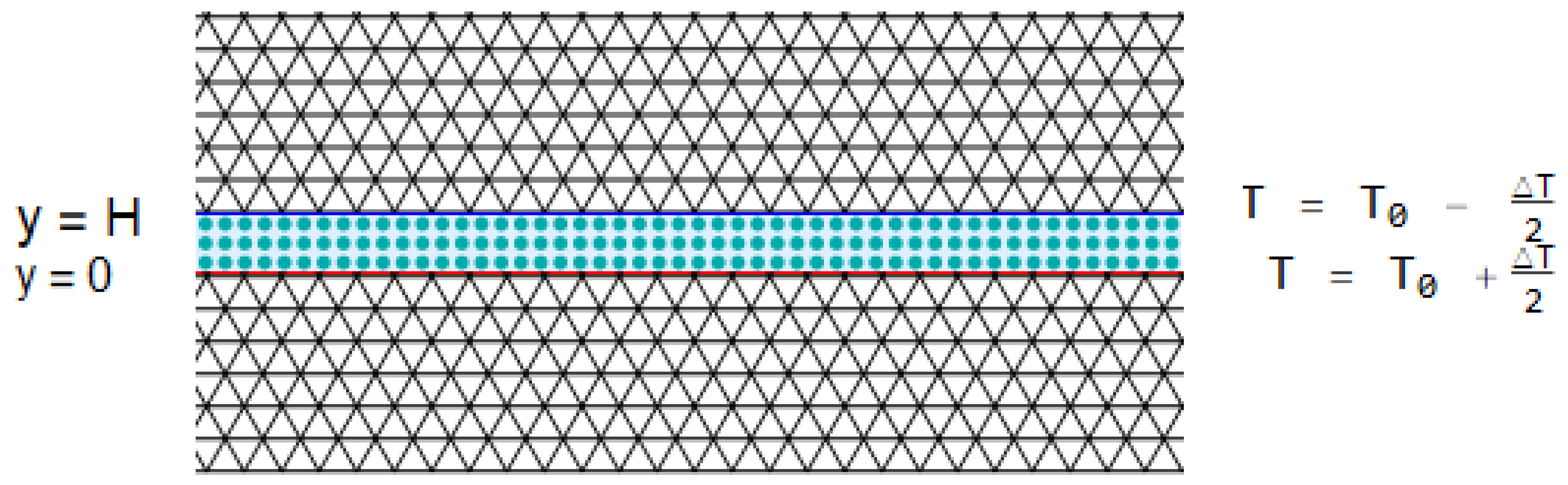
2. Mathematical Formulation

We consider the RBCS in a layer of a sparsely packed porous medium saturated with a Newtonian liquid between two densely packed porous slabs at $y=0$ and $y=H$. The lower- and upper-horizontal walls are maintained at constant temperatures of $T_0$ + $\mathsf{\Delta }T$ and $T_0$, respectively. The regions outside of the domain of interest, $y>H$ and $y<0$, are assumed to be tightly packed porous media. As a result, these regions can exchange both liquid matter and heat with the domain of interest. The Cartesian coordinate system is chosen. A schematic of the described problem is presented in Figure 1.

As shown in the planar diagram in Figure 1, the analysis is restricted to 2D rolls, which means that the dynamics in any plane parallel to the $xz$ plane will be identical; in other words, the physical quantities do not depend on the spatial variable z. The components of the velocity vector $\overrightarrow{q}$ in this 2D setup are taken to be $(u,v)$, respectively, in the x and y directions. It is further assumed that the solid and liquid phases of the considered problem are in local thermal equilibrium and that the porous media possess homogeneous properties in both directions. In addition, the dissipation due to viscosity is assumed to be negligibly small. Under such assumptions, one can invoke Oberbeck–Boussinesq approximation to write the governing equations in the following form:

$$\begin{array}{c}\nabla ·\overrightarrow{q}=0,\hspace{1em}\hspace{1em}\hspace{1em}\hspace{1em}\hspace{1em}\hspace{1em}\hspace{1em}\hspace{1em}\hspace{1em}\hspace{1em}\hspace{1em}\hspace{1em}\hspace{1em}\hspace{1em}\hspace{1em}\hspace{1em}\hspace{1em}\hspace{1em}\hspace{1em}\hspace{1em}\hspace{1em}\hfill \end{array}$$

(1)

$$\begin{array}{c}\frac{{\rho }_0}{\varphi }\left[\frac{\partial \overrightarrow{q}}{\partial t}+\frac{1}{\varphi }\left(\overrightarrow{q}·\nabla \right)\overrightarrow{q}\right]=-\nabla p+\tilde{\mu }{\nabla }^2\overrightarrow{q}+{\rho }_0\beta \left(T-T_0\right)g\widehat{j}-\frac{\mu }{\mathtt{K}}\overrightarrow{q},\hfill \end{array}$$

(2)

$$\begin{array}{c}{\left({\rho }_0{C}_p\right)}_m\frac{\partial T}{\partial t}+{\left({\rho }_0{C}_p\right)}_f\left(\overrightarrow{q}·\nabla \right)T={\left({\rho }_0{C}_p\right)}_m{\kappa }_m{\nabla }^{2}T.\hspace{1em}\hspace{1em}\hspace{1em}\hspace{1em}\hspace{1em}\hfill \end{array}$$

(3)

The symbols appearing in Equations (1)–(3) are

$$\begin{array}{cc}p,\left(\mathrm{Pa}\right)& \mathrm{the}\mathrm{hydrostatic}\mathrm{pressure}\mathrm{of}\mathrm{the}\mathrm{liquid},\hfill \\ \mu ,{(\mathrm{kgm}}^{-1}{\mathrm{s}}^{-1})& \mathrm{the}\mathrm{dynamic}\mathrm{viscosity}\mathrm{of}\mathrm{the}\mathrm{liquid},\hfill \\ \tilde{\mu },{(\mathrm{kgm}}^{-1}{\mathrm{s}}^{-1})& \mathrm{the}\mathrm{effective}\mathrm{viscosity},\hfill \\ \mathtt{K},\left({\mathrm{m}}^2\right)& \mathrm{the}\mathrm{permeability}\mathrm{of}\mathrm{the}\mathrm{porous}\mathrm{matrix},\hfill \\ {\rho }_0,\left({\mathrm{kgm}}^{-3}\right)& \mathrm{the}\mathrm{reference}\mathrm{density}\mathrm{of}\mathrm{the}\mathrm{liquid},\hfill \\ \beta ,\left({\mathrm{K}}^{-1}\right)& \mathrm{the}\mathrm{coefficient}\mathrm{of}\mathrm{thermal}\mathrm{expansion},\hfill \\ g,\left({\mathrm{ms}}^{-2}\right)& \mathrm{the}\mathrm{acceleration}\mathrm{due}\mathrm{to}\mathrm{gravity},\hfill \\ T,\left(\mathrm{K}\right)& \mathrm{the}\mathrm{temperature},\hfill \\ T_0,\left(\mathrm{K}\right)& \mathrm{the}\mathrm{reference}\mathrm{temperature},\hfill \\ {\displaystyle {\kappa }_m=\frac{k_m}{{\left({\rho }_0{C}_p\right)}_m},\left({\mathrm{m}}^2{\mathrm{s}}^{-1}\right)}& \mathrm{the}\mathrm{effective}\mathrm{thermal}\mathrm{diffusivity}\mathrm{of}\mathrm{the}\mathrm{interior}\mathrm{porous}\mathrm{matrix},\hfill \\ k_m,\left({\mathrm{Wm}}^{-1}{\mathrm{K}}^{-1}\right)& \mathrm{the}\mathrm{thermal}\mathrm{conductivity}\mathrm{of}\mathrm{the}\mathrm{interior}\mathrm{porous}\mathrm{matrix},\hfill \\ {\left({\rho }_0{C}_p\right)}_m,\left(\mathrm{J}{\mathrm{m}}^{-3}{\mathrm{K}}^{-1}\right)& \mathrm{the}\mathrm{average}\mathrm{volumetric}\mathrm{heat}\mathrm{capacity}\mathrm{of}\mathrm{the}\mathrm{interior}\mathrm{porous}\mathrm{matrix},\hfill \\ {\left({\rho }_0{C}_p\right)}_f,\left(\mathrm{J}{\mathrm{m}}^{-3}{\mathrm{K}}^{-1}\right)& \mathrm{the}\mathrm{average}\mathrm{volumetric}\mathrm{heat}\mathrm{capacity}\mathrm{of}\mathrm{the}\mathrm{liquid},\hfill \\ C_p,\left(\mathrm{J}{\mathrm{kg}}^{-1}{\mathrm{K}}^{-1}\right)& \mathrm{the}\mathrm{specific}\mathrm{heat}\mathrm{at}\mathrm{constant}\mathrm{pressure},\hfill \\ \varphi ,(0<\varphi <1)& \mathrm{the}\mathrm{volume}\mathrm{fraction}.\hfill \end{array}$$

It is assumed that the domain of interest, $0<y<H$, exchanges heat with the lower region, $y<0$, through convection with an out flux proportional to $T_0+{\displaystyle \frac{\mathsf{\Delta }T}{2}}$, with $\mathsf{\Delta }T>0$, and with the upper region, $y>H$, with an out flux proportional to $T_0-{\displaystyle \frac{\mathsf{\Delta }T}{2}}$. The horizontal walls $y=0$ and $y=H$ are assumed to have different heat transfer coefficient values $h_l$ and $h_u$, respectively. The walls $y=0$ and $y=H$ are also assumed to be permeable, with different permeabilities, ${\mathtt{K}}_l^{*}$ and ${\mathtt{K}}_u^{*}$, respectively. Since the boundaries are permeable, the normal mass flux is continuous, and the tangential component of the seepage velocity $\overrightarrow{q}=(u,v)$ must satisfy the empirical relationship of the Beavers and Joseph [19] or the Saffman [21] slip condition. Thus, the boundary conditions are modeled as follows [29,34]:

$$\begin{array}{c}\hfill \left.\begin{array}{c}\hfill v=0,\frac{\partial u}{\partial y}-\frac{\alpha u}{\sqrt{{\mathtt{K}}_l^{*}}}=0,\frac{\partial T}{\partial y}-{\displaystyle \frac{h_l}{k_m}}\left[T-\left(T_0+\frac{\mathsf{\Delta }T}{2}\right)\right]=0\\ \hfill \mathrm{at}y=0\mathrm{for}-\infty <x<\infty ,\end{array}\right\}\end{array}$$

(4)

$$\begin{array}{c}\hfill \left.\begin{array}{c}\hfill v=0,\frac{\partial u}{\partial y}+\frac{\alpha u}{\sqrt{{\mathtt{K}}_u^{*}}}=0,\frac{\partial T}{\partial y}+{\displaystyle \frac{h_u}{k_m}}\left[T-\left(T_0-\frac{\mathsf{\Delta }T}{2}\right)\right]=0\\ \hfill \mathrm{at}y=H\mathrm{for}-\infty <x<\infty .\end{array}\right\}\end{array}$$

(5)

The third-kind temperature boundary conditions in (4) and (5) arise due to a modified version of Newton’s law of cooling. The third-kind velocity boundary conditions are due to the Saffman version of the Beavers–Joseph law [19,21]. The material parameters characterizing the structure of the porous matrix at the boundaries determine the non-dimensional constant $\alpha$ (slip coefficient) that appears in Equations (4) and (5). At this juncture, it should be noted that the analysis is restricted to small-scale convective motions in a sparsely packed, porous medium, and hence the convective acceleration term, $(\overrightarrow{q}·\nabla )\overrightarrow{q}$, in Equation (2) can be neglected, in comparison with the heat advection term $(\overrightarrow{q}·\nabla )T$ in Equation (3). This essentially means that thermally induced instabilities dominate the hydrodynamic instabilities. Furthermore, in the case of a viscous liquid, in the absence of an applied force, a material particle retains its momentum when it is displaced from one point to another. However, in a porous medium with a fixed solid matrix, this is not the case, as the solid matrix obstructs the motion, resulting in momentum variation. With the assumption of small-scale convective motions, many studies have considered the convective acceleration term, $(\overrightarrow{q}·\nabla )\overrightarrow{q}$, to be quite small and hence dropped it from the study [3,8]. The dimensionless variables used in this study are given by

$$\left.\begin{array}{c}(x^{*},y^{*})={\displaystyle \frac{1}{H}}(x,y),t^{*}={\displaystyle \frac{{\kappa }_m}{H^2}}t,\\ {\overrightarrow{q}}^{*}=(u^{*},v^{*})={\displaystyle \frac{MH}{{\kappa }_m}}(u,v)={\displaystyle \frac{MH}{{\kappa }_m}}\overrightarrow{q},\\ p^{*}={\displaystyle \frac{M{H}^2}{\mu {\kappa }_m}}p,T^{*}={\displaystyle \frac{T-T_0}{\mathsf{\Delta }T}}\end{array}\right\},$$

(6)

where ${\displaystyle M={\left({\rho }_0{C}_p\right)}_f/{\left({\rho }_0{C}_p\right)}_m}$ is the heat capacity ratio.

Using Equation (6) in (1)–(5), and dropping the asterisks for simplicity, the non-dimensional form of the governing equations may be written as

$$\begin{array}{c}\nabla ·\overrightarrow{q}=0,\hspace{1em}\hspace{1em}\hspace{1em}\hspace{1em}\hspace{1em}\hspace{1em}\hspace{1em}\hspace{1em}\hspace{1em}\hspace{1em}\hspace{1em}\hfill \end{array}$$

(7)

$$\begin{array}{c}\frac{1}{P{r}^{*}}\frac{\partial \overrightarrow{q}}{\partial t}=-\nabla p+\mathsf{\Lambda }{\nabla }^2\overrightarrow{q}-{\sigma }^2\overrightarrow{q}+RaT\widehat{j},\hfill \end{array}$$

(8)

$$\begin{array}{c}\frac{\partial T}{\partial t}+(\overrightarrow{q}·\nabla )T={\nabla }^{2}T,\hspace{1em}\hspace{1em}\hspace{1em}\hspace{1em}\hspace{1em}\hspace{1em}\hfill \end{array}$$

(9)

and the boundary conditions in the dimensionless form as

$$\begin{array}{c}\hfill \left.\begin{array}{c}\hfill v=0,\frac{\partial u}{\partial y}-S_{l}u=0,\frac{\partial T}{\partial y}-B{i}_l\left(T-\frac{1}{2}\right)=0\\ \hfill \mathrm{at}y=0\mathrm{for}-\infty <x<\infty ,\end{array}\right\}\end{array}$$

(10)

$$\begin{array}{c}\hfill \left.\begin{array}{c}\hfill v=0,\frac{\partial u}{\partial y}+S_{u}u=0,\frac{\partial T}{\partial y}+B{i}_u\left(T+\frac{1}{2}\right)=0\\ \hfill \mathrm{at}y=1\mathrm{for}-\infty <x<\infty \end{array}\right\}.\end{array}$$

(11)

The non-dimensional numbers appearing in Equations (7)–(11) are as follows: ${\displaystyle P{r}^{*}=\varphi \lambda Pr}$ is the modified Prandtl number, ${\displaystyle Pr=\frac{\mu }{{\rho }_0{\kappa }_f}}$ is the Prandtl number, ${\displaystyle \lambda =\frac{{\kappa }_f}{{\kappa }_m}}$ is the thermal diffusivity ratio, ${\displaystyle \varphi }$ is the porosity, ${\displaystyle \mathsf{\Lambda }=\frac{\tilde{\mu }}{\mu }}$ is the viscosity ratio, ${\displaystyle {\sigma }^2=\frac{H^2}{\mathtt{K}}}$ is the inverse Darcy number or the porous parameter, ${\displaystyle R{a}_f=\frac{{\rho }_{0}g\beta \mathsf{\Delta }T{H}^3}{\mu {\kappa }_f}}$ is the Rayleigh number, ${\displaystyle Ra=\lambda MR{a}_f}$ is the modified Rayleigh number, ${\displaystyle (S_l,S_u)=\left(\frac{\alpha H}{\sqrt{{\mathtt{K}}_l^{*}}},\frac{\alpha H}{\sqrt{{\mathtt{K}}_u^{*}}}\right)}$ are the slip Darcy numbers at lower and upper plates, respectively, and ${\displaystyle (B{i}_l,B{i}_u)=\left(\frac{h_{l}H}{k_m},\frac{h_{u}H}{k_m}\right)}$ are the Biot numbers at lower and upper plates, respectively.

It should be noted here that

(a)

the limiting case $(B{i}_l,B{i}_u)\to (\infty ,\infty )$ recovers the isothermal horizontal boundaries, while $(B{i}_l,B{i}_u)\to (0,0)$ recovers adiabatic horizontal boundaries, and

(b)

the limiting case $(S_l,S_u)\to (0,0)$ recovers stress free horizontal boundaries, while $(S_l,S_u)\to (\infty ,\infty )$ recovers the rigid horizontal boundaries.

The governing Equations (7)–(9) can be written in component form, as follows:

$$\begin{array}{c}\frac{\partial u}{\partial x}+\frac{\partial v}{\partial y}=0,\hspace{1em}\hspace{1em}\hspace{1em}\hspace{1em}\hspace{1em}\hspace{1em}\hspace{1em}\hspace{1em}\hspace{1em}\hspace{1em}\hspace{1em}\hspace{1em}\hspace{1em}\hfill \end{array}$$

(12)

$$\begin{array}{c}\frac{1}{P{r}^{*}}\frac{\partial u}{\partial t}=-\frac{\partial p}{\partial x}+\mathsf{\Lambda }\left(\frac{{\partial }^{2}u}{\partial x^2}+\frac{{\partial }^{2}u}{\partial y^2}\right)-{\sigma }^{2}u,\hspace{1em}\hspace{1em}\hspace{1em}\hfill \end{array}$$

(13)

$$\begin{array}{c}\frac{1}{P{r}^{*}}\frac{\partial v}{\partial t}=-\frac{\partial p}{\partial y}+\mathsf{\Lambda }\left(\frac{{\partial }^{2}v}{\partial x^2}+\frac{{\partial }^{2}v}{\partial y^2}\right)-{\sigma }^{2}v+RaT,\hfill \end{array}$$

(14)

$$\begin{array}{c}\frac{\partial T}{\partial t}+u\frac{\partial T}{\partial x}+v\frac{\partial T}{\partial y}=\frac{{\partial }^{2}T}{\partial x^2}+\frac{{\partial }^{2}T}{\partial y^2}.\hspace{1em}\hspace{1em}\hspace{1em}\hspace{1em}\hspace{1em}\hfill \end{array}$$

(15)

The stream function, $\psi (x,y)$, is constant in the following form, so as to satisfy the continuity Equation (12):

$$u=-\frac{\partial \psi }{\partial y},\hspace{1em}\hspace{1em}\hspace{1em}\hspace{1em}v=\frac{\partial \psi }{\partial x}.$$

(16)

Eliminating the pressure between Equations (13) and (14), and using Equation (16) in the resulting equation, the governing Equations (13)–(15) reduce to:

$$\begin{array}{c}\frac{1}{P{r}^{*}}\frac{\partial }{\partial t}\left({\nabla }^2\psi \right)=\mathsf{\Lambda }{\nabla }^4\psi -{\sigma }^2{\nabla }^2\psi +Ra\frac{\partial T}{\partial x},\hfill \end{array}$$

(17)

$$\begin{array}{c}\frac{\partial T}{\partial t}+\frac{\partial (\psi ,T)}{\partial (x,y)}={\nabla }^{2}T.\hspace{1em}\hspace{1em}\hspace{1em}\hspace{1em}\hspace{1em}\hspace{1em}\hfill \end{array}$$

(18)

Here ${\nabla }^2={\displaystyle \frac{{\partial }^2}{\partial x^2}}+{\displaystyle \frac{{\partial }^2}{\partial y^2}}$ is the Laplacian operator. The second term on the left-hand side of Equation (18) is the Jacobian term. Now, the boundary conditions (10) and (11) take the following form:

$$\begin{array}{c}\hfill \begin{array}{c}\hfill \psi =0,\frac{{\partial }^2\psi }{\partial y^2}-S_l\frac{\partial \psi }{\partial y}=0,\frac{\partial T}{\partial y}-B{i}_l\left(T-\frac{1}{2}\right)=0\mathrm{at}y=0\mathrm{for}-\infty <x<\infty \end{array},\end{array}$$

(19)

$$\begin{array}{c}\hfill \begin{array}{c}\hfill \psi =0,\frac{{\partial }^2\psi }{\partial y^2}+S_u\frac{\partial \psi }{\partial y}=0,\frac{\partial T}{\partial y}+B{i}_u\left(T+\frac{1}{2}\right)=0\mathrm{at}y=1\mathrm{for}-\infty <x<\infty \end{array}.\end{array}$$

(20)

Siddheshwar [34] reported detailed information on the derivation of the rough boundary condition mentioned above, while Platten and Legros [39] gave similar information on the Robin boundary condition for temperature.

2.1. Basic State

The heat is transferred solely in the conduction mode in the quiescent basic state, and one can obtain the following stationary solution for Equations (17) and (18), corresponding to the basic state, as follows:

$${\psi }_b=0,\hspace{1em}\hspace{1em}\hspace{1em}{T}_b\left(y\right)=-{\mathtt{B}}_{\mathrm{eff}}\left[y-\frac{1}{2}\left({\displaystyle \frac{1}{{\mathtt{B}}_{\mathrm{eff}}}}-{\displaystyle \frac{2}{B{i}_l}}\right)\right],$$

(21)

where the subscript, b, denotes a basic state quantity and ${\mathtt{B}}_{\mathrm{eff}}=B{i}_{l}B{i}_u/(B{i}_l+B{i}_u+B{i}_{l}B{i}_u)$ is the effective Biot number.

Noting that $u_b=0,v_b=0$ and $p_b=p_b\left(y\right)$ in the basic state, from Equation (14) we obtain

$$\frac{d{p}_b}{dy}=Ra{T}_b\left(y\right).$$

(22)

Equation (13) is trivially satisfied in the basic state. Substituting Equation (21) in (22) and integrating with respect to y once, we obtain

$$p_b\left(y\right)=p_0-Ra{\mathtt{B}}_{\mathrm{eff}}\left[\frac{y^2}{2}-\frac{y}{2}\left({\displaystyle \frac{1}{{\mathtt{B}}_{\mathrm{eff}}}}-{\displaystyle \frac{2}{B{i}_l}}\right)\right].$$

(23)

The quantity $p_0$ in Equation (23) is an arbitrary integration constant.

2.2. Perturbations of the Basic-State

The basic state given by Equation (21) is perturbed by thermal perturbations, resulting in a change in the physical quantities, as follows:

$$\left.\begin{array}{c}\psi ={\psi }_b+\mathsf{\Psi },\\ T=T_b\left(y\right)+\mathsf{\Theta },\end{array}\right\}$$

(24)

where $\mathsf{\Psi }$ and $\mathsf{\Theta }$ are perturbations in the stream function and temperature, respectively. These perturbations have a small amplitude and finite amplitude in the case of linear and nonlinear stability analyses, respectively. Substituting Equation (24) into Equations (17) and (18), the governing equations for the disturbances take the form:

$$\begin{array}{c}\frac{1}{P{r}^{*}}\frac{\partial }{\partial t}\left({\nabla }^2\mathsf{\Psi }\right)=\mathsf{\Lambda }{\nabla }^4\mathsf{\Psi }-{\sigma }^2{\nabla }^2\mathsf{\Psi }+Ra\frac{\partial \mathsf{\Theta }}{\partial x},\hfill \end{array}$$

(25)

$$\begin{array}{c}\frac{\partial \mathsf{\Theta }}{\partial t}+{\displaystyle \frac{\partial (\mathsf{\Psi },\mathsf{\Theta })}{\partial (x,y)}}-{\mathtt{B}}_{\mathrm{eff}}\frac{\partial \mathsf{\Psi }}{\partial x}={\nabla }^2\mathsf{\Theta }.\hspace{1em}\hspace{1em}\hspace{1em}\hfill \end{array}$$

(26)

The boundary conditions for solving Equations (25) and (26) are obtained from Equations (19)–(21), (23), and (24), and now take the form:

$$\begin{array}{c}\hfill \begin{array}{c}\hfill \mathsf{\Psi }=0,\frac{{\partial }^2\mathsf{\Psi }}{\partial y^2}-S_l\frac{\partial \mathsf{\Psi }}{\partial y}=0,\frac{\partial \mathsf{\Theta }}{\partial y}-B{i}_l\mathsf{\Theta }=0\mathrm{at}y=0\mathrm{for}-\infty <x<\infty \end{array},\end{array}$$

(27)

$$\begin{array}{c}\hfill \begin{array}{c}\hfill \mathsf{\Psi }=0,\frac{{\partial }^2\mathsf{\Psi }}{\partial y^2}+S_u\frac{\partial \mathsf{\Psi }}{\partial y}=0,\frac{\partial \mathsf{\Theta }}{\partial y}+B{i}_u\mathsf{\Theta }=0\mathrm{at}y=1\mathrm{for}-\infty <x<\infty \end{array}.\end{array}$$

(28)

The periodicity condition dictated by the formation of the Brinkman–Bénard convective cells is given by

$$\begin{array}{c}\hfill \left.\begin{array}{ccc}\hfill \mathsf{\Psi }\left(a\pi \left(x+\frac{2}{a}\right),y\right)& =\hfill & \hfill \mathsf{\Psi }\left(x,y\right)\\ \hfill \mathsf{\Theta }\left(a\pi \left(x+\frac{2}{a}\right),y\right)& =\hfill & \hfill \mathsf{\Theta }\left(x,y\right)\end{array}\right\},\mathrm{for}0<y<1\end{array}$$

(29)

The above periodicity condition and the assumption of an infinite-horizontal-extent BBCS indicates the symmetry of the system about the vertical lines in the $xy$-plane, at the edge of a pair of counter rotating cells. In view of the fact that symmetry is invoked through the periodicity condition (29), there is no need to specify the $x$-boundary condition (due to absence of lateral walls).

2.3. Linear Stability Analysis of the Marginal State

In order to prove the validity of the principle of exchange of stabilities in the case of general boundary conditions, we consider the following periodic wave solutions of Equations (25) and (26):

$$\left.\begin{array}{c}{\displaystyle \mathsf{\Psi }(x,y)=A{e}^{i\omega t}sin\left(\pi ax\right)F\left(y\right),}\\ {\displaystyle \mathsf{\Theta }(x,y)={\mathtt{B}}_{\mathrm{eff}}B{e}^{i\omega t}cos\left(\pi ax\right)G\left(y\right),}\end{array}\right\}$$

(30)

where $F\left(y\right)$ and $G\left(y\right)$ are determined, so as to satisfy the boundary conditions (27) and (28). The periodicity condition (29) is obviously satisfied by Equation (30). In the Appendix A, we have proven the principle of exchange of stabilities, and hence we can set $\omega =0$. Now substituting Equation (30) with $\omega =0$ in Equations (25) and (26), we obtain

$$\begin{array}{c}\mathsf{\Lambda }{F}^{\prime \prime \prime \prime }-(2{\pi }^2{a}^2\mathsf{\Lambda }+{\sigma }^2)F^{\prime \prime }+({\pi }^2{a}^2\mathsf{\Lambda }+{\sigma }^2){\pi }^2{a}^{2}F-\pi aR{a}^{*}G=0,\hspace{1em}\hspace{1em}\hspace{1em}\hspace{1em}\hfill \end{array}$$

(31)

$$\begin{array}{c}{G}^{\prime \prime }-{\pi }^2{a}^{2}G+\pi aF=0,\hspace{1em}\hspace{1em}\hspace{1em}\hspace{1em}\hspace{1em}\hspace{1em}\hspace{1em}\hspace{1em}\hspace{1em}\hspace{1em}\hspace{1em}\hspace{1em}\hspace{1em}\hspace{1em}\hspace{1em}\hspace{1em}\hspace{1em}\hspace{1em}\hspace{1em}\hspace{1em}\hfill \end{array}$$

(32)

where the differentiation with respect to-y is denoted by the prime.

The boundary conditions (27) and (28), together with Equation (30), lead to

$$\begin{array}{c}F=0,F^{\prime \prime }-S_l{F}^{\prime }=0,G^{\prime }-B{i}_{l}G=0\mathrm{at}y=0,\hfill \end{array}$$

(33)

$$\begin{array}{c}F=0,F^{\prime \prime }+S_u{F}^{\prime }=0,G^{\prime }+B{i}_{u}G=0\mathrm{at}y=1.\hfill \end{array}$$

(34)

In Equations (31)–(34), the modified Rayleigh number, $R{a}^{*}=Ra{\mathtt{B}}_{\mathrm{eff}}$, is the eigenvalue of the problem. We first solve BEVP (31)–(34) using the shooting method, to determine the critical wave number, $a_c$, and the critical Darcy–Rayleigh number, ${R{a}^{*}}_c$. This information is then used to obtain a Maclaurin series expansion for the corresponding eigenfunctions. The eigenfunctions must be chosen appropriately, in order to meet the orthogonality conditions required by the weakly nonlinear stability analysis. The following section highlights the implementation of the shooting method for solving the BEVP (31)–(34).

3. Solution of the BEVP of the Linear Stability Analysis

3.1. Evaluation of Unknown, Initial, and Critical Values Using the Shooting Method

To solve the BEVP using the shooting method, we assume the eigenvalue, $R{a}^{*}$, is an additional variable. Following Siddheshwar and Revathi [40], we introduce the following additional artificial differential equation into the boundary value problem:

$$\frac{d}{dy}\left(R{a}^{*}\right)=0,R{a}^{*}\left(0\right)=R{a}^{*}$$

(35)

and a normalized additional initial condition, such as

$$G\left(0\right)=1$$

(36)

It should be noted here that the eigenfunctions depend on the normalization condition used. Any of the following conditions could also be used in place of condition (36):

$$F^{\prime }\left(0\right)=1\mathrm{or}{F}^{\prime \prime }\left(0\right)=1\mathrm{or}{G}^{\prime }\left(0\right)=1.$$

(37)

We chose the normalization condition (36) so that the eigenfunctions satisfy the orthogonality conditions required by the weakly nonlinear analysis. Now, by treating the eigenvalue as an additional variable, Equations (31)–(34) together with (35) and (36) constitute an augmented boundary value problem (ABVP). To solve this BVP using the shooting method, we first convert the ABVP into an equivalent initial value problem (IVP) through introducing the necessary unavailable initial conditions $F^{\prime }\left(0\right)={\alpha }^{*}$ and $F^{\prime \prime \prime }\left(0\right)={\beta }^{*}$ in the place of the right-end boundary conditions. Thus, we have the following "augmented" IVP in place of the ABVP constituted by Equations (31)–(36):

$$\left.\begin{array}{c}{\displaystyle \frac{d{u}_1}{dy}}=u_2,u_1\left(0\right)=0;{\displaystyle \frac{d{u}_2}{dy}}=u_3,u_2\left(0\right)={\alpha }^{*};\hfill \\ {\displaystyle \frac{d{u}_3}{dy}}=u_4,u_3\left(0\right)={\alpha }^{*}{S}_l;\hfill \\ {\displaystyle \frac{d{u}_4}{dy}}={\displaystyle \frac{1}{\mathsf{\Lambda }}}\left[\left(2{\pi }^2{a}^2\mathsf{\Lambda }+{\sigma }^2\right)u_3-\left({\pi }^2{a}^2\mathsf{\Lambda }+{\sigma }^2\right){\pi }^2{a}^2{u}_1\right.\hfill \\ \left.+\pi a{u}_5{u}_7\right],u_4\left(0\right)={\beta }^{*};\hfill \\ {\displaystyle \frac{d{u}_5}{dy}}=u_6,u_5\left(0\right)=1;\hfill \\ {\displaystyle \frac{d{u}_6}{dy}}={\pi }^2{a}^2{u}_5-\pi a{u}_1,u_6\left(0\right)=B{i}_l;\hfill \\ {\displaystyle \frac{d{u}_7}{dy}}=0,u_7\left(0\right)=R{a}^{*}.\hfill \end{array}\right\}$$

(38)

Here, $u_1$, $u_5$, and $u_7$ stand for the variables $F\left(y\right)$, $G\left(y\right)$, and $R{a}^{*}$, respectively. The IVP (38) needs to be solved iteratively, until the right-end boundary conditions (34) are satisfied.

To implement a correction scheme for the guessed values of ${\alpha }^{*}$, ${\beta }^{*}$ and $R{a}^{*}$, three additional IVPs are formed by differentiating (38) with respect to ${\alpha }^{*}$, ${\beta }^{*}$, and $R{a}^{*}$. Thus, four IVPs are solved using the Runge–Kutta–Fehlberg (RKF45) method, using an adaptive step size, for an assumed guess value of ${\alpha }^{*}$, ${\beta }^{*}$ and $R{a}^{*}$ to obtain refined values of ${\alpha }^{*}$, ${\beta }^{*}$, and $R{a}^{*}$. This procedure needs to be repeated until the residues are minimized to the desired tolerance. Rough estimates for the initial values, to begin with, may be obtained using the single-term Galerkin method, as described in Siddheshwar and Revathi [40]. Post-convergence, the eigenvalue, $R{a}^{*}$, is recorded over a range of values of the wave number, a, for a particular set of parameter values. These data can be used to find the minimum value ${R{a}^{*}}_c$ of the eigenvalue and the corresponding wave number, $a_c$, which are known as critical values.

3.2. Discussion of the Normalization Condition and "Barletta Scaling"

It should be reiterated that the eigenfunctions required by the weakly nonlinear stability analysis must satisfy the orthogonality conditions. This mainly depends on the assumed normalization condition, which in turn is sensitive to the type of lower boundary. This essentially means that we must choose an appropriate normalization condition to meet the orthogonality constraints. Extensive computational experimentation revealed that for small/large values $B{i}_l$, we may have to float $B{i}_l$ in the initial conditions between $G\left(0\right)$ and $G^{\prime }\left(0\right)$; and similarly, for small/large-values of $S_l$, we may have to float $S_l$ in the initial conditions between $F^{\prime }\left(0\right)$ and $F^{\prime \prime }\left(0\right)$. Table 1 summarizes the appropriate normalization condition, along with the other initial conditions used in various situations.

Table 1. Initial conditions and appropriate normal condition (appears in bold font) for various types of lower boudary.

Type of Lower Boundary	Initial and Normalization Condition
Free-Isothermal (FIFI, FIFA, FIRI, FIRA)	$u_1\left(0\right)=0,{\mathbf{u}}_{\mathbf{2}}\left(\mathbf{0}\right)=\mathbf{1},u_3\left(0\right)=S_l,u_4\left(0\right)={\alpha }^{*}$,
$S_l\to 0,B{i}_l\to \infty$	$u_5\left(0\right)={\displaystyle \frac{{\beta }^{*}}{B{i}_l}},u_6\left(0\right)={\beta }^{*},u_7\left(0\right)=R{a}^{*}$.
Free-Adiabatic (FAFI, FAFA, FARI, FARA)	$u_1\left(0\right)=0,{\mathbf{u}}_{\mathbf{2}}\left(\mathbf{0}\right)=\mathbf{1},u_3\left(0\right)=S_l,u_4\left(0\right)={\alpha }^{*}$,
$S_l\to 0,B{i}_l\to 0$	$u_5\left(0\right)={\beta }^{*},u_6\left(0\right)={\beta }^{*}B{i}_l,u_7\left(0\right)=R{a}^{*}$.
Rigid-Isothermal (RIFI, RIFA, RIRI, RIRA)	$u_1\left(0\right)=0,u_3\left(0\right)={\displaystyle \frac{1}{S_l}},{\mathbf{u}}_{\mathbf{3}}\left(\mathbf{0}\right)=\mathbf{1},u_4\left(0\right)={\alpha }^{*}$,
$S_l\to \infty ,B{i}_l\to \infty$	$u_5\left(0\right)={\displaystyle \frac{{\beta }^{*}}{B{i}_l}},u_6\left(0\right)={\beta }^{*},u_7\left(0\right)=R{a}^{*}$.
Rigid-Adiabatic (RAFI, RAFA, RARI, RARA)	$u_1\left(0\right)=0,u_3\left(0\right)={\displaystyle \frac{1}{S_l}},{\mathbf{u}}_{\mathbf{3}}\left(\mathbf{0}\right)=\mathbf{1},u_4\left(0\right)={\alpha }^{*}$,
$S_l\to \infty ,B{i}_l\to 0$	$u_5\left(0\right)={\beta }^{*},u_6\left(0\right)={\beta }^{*}B{i}_l,u_7\left(0\right)=R{a}^{*}$.

It can be seen that the temperature distribution, $\mathsf{\Theta }(x,y)$, has been scaled by ${\mathtt{B}}_{\mathrm{eff}}$. This ensures that ${\mathtt{B}}_{\mathrm{eff}}$, which is the necessary basic state temperature gradient, does not appear in the BEVP (31)–(34) and also leads to rescaling of the Rayleigh number. This is crucial in handling the limiting case of adiabatic boundaries. Note that the case of both boundaries being adiabatic results in an indeterminate value for ${\mathtt{B}}_{\mathrm{eff}}$, and if the BEVP (31)–(34) contains ${\mathtt{B}}_{\mathrm{eff}}$, then the computation will result in incorrect eigenvalues. Such a scaling turns out to be very effective in handling limiting cases and capturing accurate eigenvalues. It was introduced for the first time by Barletta and Storesletten [29], and hence we shall refer to this scaling as “Barletta scaling”. Barletta scaling may also be appropriately used for the velocity field.

We now highlight the methodology for obtaining an analytical expression for the eigenfunction, obtained numerically using the shooting method.

3.3. Series Expansion of Eigenfunctions

We use the information about the unavailable initial conditions and critical values of $Ra$ and a obtained using the shooting method in constructing a Maclaurin series for the eigenfunctions. Before proceeding further, we note here that the series solution procedure adopted by Narayana et al. [35] for solving the BEVP (31)–(34) is laborious when determining the critical values $a_c$ and ${R{a}^{*}}_c$. In their work, for each wave number, we need to solve the nonlinear algebraic system of three equations (generated using the right-end boundary conditions (34)) using Newton’s method and obtain the values of ${\alpha }^{*},{\beta }^{*}$ and $R{a}^{*}$, which renders the procedure relatively difficult. Here, we adopt a much simpler procedure for evaluating the initial and critical values, using the shooting method, and use it to construct the series solution for the eigenfunctions. To this end we assume Maclaurin series expansion for the eigenfunctions $F\left(y\right)$ and $G\left(y\right)$, in the following form:

$$\left.\begin{array}{c}{\displaystyle F\left(y\right)=\sum _{k=0}^{\infty }{\mathfrak{a}}_k{y}^k,}\\ {\displaystyle G\left(y\right)=\sum _{k=0}^{\infty }{\mathfrak{b}}_k{y}^k,}\end{array}\right\}$$

(39)

where the Maclaurin constants ${\mathfrak{a}}_k$ and ${\mathfrak{b}}_k$ are determined by substituting (39) in the IVP defined by Equations (35)–(38). We obtain the following recurrence relations for the Maclaurin constants ${\mathfrak{a}}_k$ and ${\mathfrak{b}}_k$:

$$\begin{array}{l}(k+4)(k+3)(k+2)(k+1){\mathfrak{a}}_{k+4}-\left({\sigma }^2+2{\pi }^2{a}^2\mathsf{\Lambda }\right)(k+2)(k+1){\mathfrak{a}}_{k+2}\\ +{\pi }^2{a}^2\left({\sigma }^2+{\pi }^2{a}^2\mathsf{\Lambda }\right){\mathfrak{a}}_k-\pi aR{a}^{*}{\mathfrak{b}}_k=0\end{array}$$

(40)

$$\begin{array}{c}(k+2)(k+1){\mathfrak{b}}_{k+2}-{\pi }^2{a}^2{\mathfrak{b}}_k+\pi a{\mathfrak{a}}_k=0\hspace{1em}\hspace{1em}\hspace{1em}\hspace{1em}\hspace{1em}\hspace{1em}\hspace{1em}\hspace{1em}\hspace{1em}\hspace{1em}\hspace{1em}\hfill \end{array}$$

(41)

The first few Maclaurin constants can be obtained from the initial conditions, and after some algebra, this procedure gives us

$$F=F({\alpha }^{*},{\beta }^{*},R{a}^{*};y)\mathrm{and}G=G({\alpha }^{*},{\beta }^{*},R{a}^{*};y),$$

in the following form:

$$\begin{array}{c}F({\alpha }^{*},{\beta }^{*},R{a}^{*};y)={\alpha }^{*}y+\frac{1}{2}{\alpha }^{*}{S}_l{y}^2+\frac{{\beta }^{*}}{6}{y}^3\hfill \\ +\frac{1}{24\mathsf{\Lambda }}\left[\left({\sigma }^2+2{\pi }^2{a}^2\mathsf{\Lambda }\right){\alpha }^{*}{S}_l+\pi aR{a}^{*}\right]y^4\hfill \\ +\frac{1}{120\mathsf{\Lambda }}\left[\left({\sigma }^2+2{\pi }^2{a}^2\mathsf{\Lambda }\right){\beta }^{*}+\pi aB{i}_{l}R{a}^{*}-{\pi }^2{a}^2{\alpha }^{*}\left({\sigma }^2+{\pi }^2{a}^2\mathsf{\Lambda }\right)\right]y^5+\dots \hfill \end{array}$$

(42)

$$\begin{array}{c}G({\alpha }^{*},{\beta }^{*},R{a}^{*};y)=1+B{i}_{l}y+\frac{1}{2}{\pi }^2{a}^2{y}^2+\frac{1}{6}\left({\pi }^2{a}^{2}B{i}_l-\pi a{\alpha }^{*}\right)y^3\hfill \\ +\frac{1}{24}\left({\pi }^4{a}^4-\pi a{\alpha }^{*}{S}_l\right)y^4+\frac{1}{120}\left({\pi }^2{a}^2\left({\pi }^2{a}^{2}B{i}_l-\pi a{\alpha }^{*}\right)-\pi a{\beta }^{*}\right)y^5+\cdots .\hfill \end{array}$$

(43)

In addition to depending on ${\alpha }^{*},{\beta }^{*},R{a}^{*}$ and y, $F({\alpha }^{*},{\beta }^{*},R{a}^{*};y)$, and $G({\alpha }^{*},{\beta }^{*},R{a}^{*};y)$ depend on the parameters of the problem, viz., $S_l,S_u,B{i}_l,B{i}_u,\mathsf{\Lambda },{\sigma }^2$, and also on the wave number a. The series expansion of the eigenfunctions given by Equations (42) and (43) would change if an alternative normalization condition was used in place of (36). The convergence of the series solution presented in Equations (42) and (43) depends on the number of terms taken. Computation reveals that we must consider at least 20 terms, in order that the eigenfunctions obtained in the series match those obtained numerically.

4. Asymptotic Analysis of Both Adiabatic Boundaries ($\mathbf{0}\le {\mathit{Bi}}_{\mathit{l}}<<\mathbf{1},\mathbf{0}\le {\mathit{Bi}}_{\mathit{u}}<<\mathbf{1})$

The BEVP (31)–(34) for the case of adiabatic boundaries after scaling the eigenfunction $G\left(y\right)$ using $\pi a$ may be written as

$$\begin{array}{c}\mathsf{\Lambda }{F}^{\prime \prime \prime \prime }-(2{\pi }^2{a}^2\mathsf{\Lambda }+{\sigma }^2)F^{\prime \prime }+({\pi }^2{a}^2\mathsf{\Lambda }+{\sigma }^2){\pi }^2{a}^{2}F-{\pi }^2{a}^{2}R{a}^{*}G=0,\hfill \end{array}$$

(44)

$$\begin{array}{c}{G}^{\prime \prime }-{\pi }^2{a}^{2}G+F=0,\hspace{1em}\hspace{1em}\hspace{1em}\hspace{1em}\hspace{1em}\hspace{1em}\hspace{1em}\hspace{1em}\hspace{1em}\hspace{1em}\hspace{1em}\hspace{1em}\hspace{1em}\hspace{1em}\hspace{1em}\hspace{1em}\hfill \end{array}$$

(45)

The boundary condition leads to:

$$\begin{array}{c}F=0,\hspace{1em}{F}^{\prime \prime }=S_l{F}^{\prime },\hspace{1em}{G}^{\prime }=0\hspace{1em}\mathrm{at}\hspace{1em}y=0,\hfill \end{array}$$

(46)

$$\begin{array}{c}F=0,\hspace{1em}{F}^{\prime \prime }=-S_u{F}^{\prime },\hspace{1em}{G}^{\prime }=0\hspace{1em}\mathrm{at}\hspace{1em}y=1.\hfill \end{array}$$

(47)

We note that the critical wave number corresponding to adiabatic boundaries is very small, and hence the solution to the BEVP (44)–(47) may be written as a series expansion, in terms of ${\pi }^2{a}^2$, as follows:

$$\begin{array}{c}\hfill \left.\begin{array}{c}F\left(y\right)=F_0\left(y\right)+{\pi }^2{a}^2{F}_1\left(y\right)+\dots ,\hfill \\ G\left(y\right)=G_0\left(y\right)+{\pi }^2{a}^2{G}_1\left(y\right)+\dots ,\hfill \end{array}\right\}\end{array}$$

(48)

Substituting (48) into Equations (44)–(47), we obtain the following boundary value problems with various orders of ${\pi }^2{a}^2$:

$$\begin{array}{l}O\left({\left({\pi }^2{a}^2\right)}^0\right):\hspace{1em}\hspace{1em}\hspace{1em}\hspace{1em}\hspace{1em}\hspace{1em}\hspace{1em}\hspace{1em}\hspace{1em}\hspace{1em}\hspace{1em}\hspace{1em}\\ \mathsf{\Lambda }{F}_0^{\prime \prime \prime \prime }-{\sigma }^2{F}_0^{\prime \prime }=0,\hspace{1em}\hspace{1em}\hspace{1em}\hspace{1em}\hspace{1em}\hspace{1em}\hspace{1em}\hspace{1em}\hspace{1em}\hspace{1em}\hspace{1em}\hspace{1em}\end{array}$$

(49)

$$\begin{array}{c}{G}_0^{\prime \prime }+F_0=0,\hspace{1em}\hspace{1em}\hspace{1em}\hspace{1em}\hspace{1em}\hspace{1em}\hspace{1em}\hspace{1em}\hspace{1em}\hspace{1em}\hfill \end{array}$$

(50)

$$\begin{array}{c}{F}_0=0,F_0^{\prime \prime }=S_l{F}_0^{\prime },G_0^{\prime }=0\mathrm{at}y=0,\hspace{1em}\hfill \end{array}$$

(51)

$$\begin{array}{c}{F}_0=0,F_0^{\prime \prime }=-S_u{F}_0^{\prime },G_0^{\prime }=0\mathrm{at}y=1.\hfill \end{array}$$

(52)

$$\begin{array}{l}O\left({\left({\pi }^2{a}^2\right)}^1\right):\hspace{1em}\hspace{1em}\hspace{1em}\hspace{1em}\hspace{1em}\hspace{1em}\hspace{1em}\hspace{1em}\hspace{1em}\\ \mathsf{\Lambda }{F}_1^{\prime \prime \prime \prime \prime }-{\sigma }^2{F}_1^{\prime \prime }=R{a}^{*}{G}_0+2\mathsf{\Lambda }{F}_0^{\prime \prime }-{\sigma }^2{F}_0,\hspace{1em}\hspace{1em}\hspace{1em}\hspace{1em}\end{array}$$

(53)

$$\begin{array}{c}{G}_1^{\prime \prime }+F_1=G_0,\hspace{1em}\hspace{1em}\hspace{1em}\hspace{1em}\hspace{1em}\hspace{1em}\hspace{1em}\hspace{1em}\hfill \end{array}$$

(54)

$$\begin{array}{c}{F}_1=0,F_1^{\prime \prime }=S_l{F}_1^{\prime },G_1^{\prime }=0\mathrm{at}y=0,\hspace{1em}\hfill \end{array}$$

(55)

$$\begin{array}{c}{F}_1=0,F_1^{\prime \prime }=-S_u{F}_1^{\prime },G_1^{\prime }=0\mathrm{at}y=1.\hfill \end{array}$$

(56)

The solution to the zeroth order perturbation problem (49)–(52) is given by

$$F_0\left(y\right)=0,G_0\left(y\right)=1.$$

(57)

The solution to the first-order perturbation problem (53)–(56) is given by

$$\begin{array}{ccc}\hfill F_1\left(y\right)& =& a_1+a_{2}y+a_{3}cosh\left({\displaystyle \frac{\sigma }{\sqrt{\mathsf{\Lambda }}}}y\right)+sinh\left(a_4{\displaystyle \frac{\sigma }{\sqrt{\mathsf{\Lambda }}}}y\right)-{\displaystyle \frac{R{a}^{*}}{2{\sigma }^2}}{y}^2,\hspace{1em}\hspace{1em}\hspace{1em}\hspace{1em}\hfill \end{array}$$

(58)

$$\begin{array}{lll}{G}_1\left(y\right)& =& 1+{\displaystyle \frac{y^2}{2}}+{\displaystyle \frac{R{a}^{*}}{{\sigma }^2}}{\displaystyle \frac{y^4}{24}}-\left[{\displaystyle \frac{a_1{y}^2}{2}}+{\displaystyle \frac{a_2{y}^3}{6}}+{\displaystyle \frac{{\sigma }^2}{\mathsf{\Lambda }}}\right.\hspace{1em}\hspace{1em}\hspace{1em}\hspace{1em}\hfill \\ & & \left.\left(a_{3}cosh\left({\displaystyle \frac{\sigma }{\sqrt{\mathsf{\Lambda }}}}y\right)+a_{4}sinh\left({\displaystyle \frac{\sigma }{\mathsf{\Lambda }}}y\right)\right)\right].\hspace{1em}\hspace{1em}\hspace{1em}\hspace{1em}\hspace{1em}\hspace{1em}\hspace{1em}\hspace{1em}\hspace{1em}\hspace{1em}\hspace{1em}\end{array}$$

(59)

The expressions for the coefficients, $a_i,(i=1,2,3,4)$, which are functions of the parameters $\mathsf{\Lambda },\sigma ,S_l,S_u$ and $R{a}^{*}$ are omitted, due to reasons of space. One of the solvability conditions

$${\int }_0^{1}R{a}^{*}{F}_0\left(y\right)dy=0$$

is satisfied trivially, and the other solvability conditions

$${\int }_0^1[1-F_1\left(y\right)]G_0\left(y\right)dy=0,$$

yield the following expression for $R{a}_c^{*}$:

$$R{a}_c^{*}={\displaystyle \frac{12{\sigma }^4\left[2S_l{S}_u{\mathsf{\Lambda }}^{3/2}+b_{1}cosh\left({\displaystyle \frac{\sigma }{\sqrt{\mathsf{\Lambda }}}}\right)+b_{2}sinh\left({\displaystyle \frac{\sigma }{\sqrt{\mathsf{\Lambda }}}}\right)\right]}{\left[b_3+b_{4}cosh\left({\displaystyle \frac{\sigma }{\sqrt{\mathsf{\Lambda }}}}\right)+b_{5}sinh\left({\displaystyle \frac{\sigma }{\sqrt{\mathsf{\Lambda }}}}\right)\right]}},$$

(60)

where

$$\begin{array}{ccc}\hfill b_1& =& {\mathsf{\Lambda }}^{1/2}[-2S_l{S}_u\mathsf{\Lambda }+(S_l+S_u){\sigma }^2],\hfill \\ \hfill b_2& =& \sigma [S_l(-1+S_u)\mathsf{\Lambda }-S_u\mathsf{\Lambda }+{\sigma }^2],\hfill \\ \hfill b_3& =& 4{\mathsf{\Lambda }}^{3/2}[6(S_l+S_u+S_l{S}_u)\mathsf{\Lambda }-(6+3S_l+3S_u+S_l{S}_u){\sigma }^2],\hfill \\ \hfill b_4& =& {\mathsf{\Lambda }}^{1/2}[-24(S_l+S_u+S_l{S}_u){\mathsf{\Lambda }}^2-8(-3+S_l{S}_u)\mathsf{\Lambda }{\sigma }^2+(S_l+S_u){\sigma }^4],\hfill \\ \hfill b_5& =& \sigma [24(S_l+S_u+S_l{S}_u){\mathsf{\Lambda }}^2+(-4(3+S_l)+(-4+S_l)S_u)\mathsf{\Lambda }{\sigma }^2+{\sigma }^4].\hfill \end{array}$$

In the limit ${\sigma }^2\to 0$ and $\mathsf{\Lambda }=1$ (Rayleigh–Bénard-convection), we obtain

$$R{a}_c^{*}={\displaystyle \frac{720[4(3+S_u)+S_l(4+S_u)]}{9(8+S_u)+S_l(9+S_u)}}.$$

(61)

5. Weakly Nonlinear Stability Analysis: Derivation of the Generalized Lorenz Model

The minimal Fourier–Galerkin representation for obtaining the generalized Lorenz model is

$$\begin{array}{ccc}\hfill \mathsf{\Psi }(x,y,t)& =& A\left(t\right)sin\left(\pi ax\right)F\left(y\right),\hspace{1em}\hspace{1em}\hspace{1em}\hspace{1em}\hspace{1em}\hspace{1em}\hspace{1em}\hfill \end{array}$$

(62)

$$\begin{array}{ccc}\hfill \mathsf{\Theta }(x,y,t)& =& {\mathtt{B}}_{\mathrm{eff}}\left\{B\left(t\right)cos\left(\pi ax\right)G\left(y\right)-C\left(t\right)H\left(y\right)\right\},\hfill \end{array}$$

(63)

where $F\left(y\right)$ and $G\left(y\right)$ are given by Equations (40) and (41), with ${\alpha }^{*}$, ${\beta }^{*}$, ${R{a}_D}_c$, and $a_c$ tabulated in Table 2 and Table 3 for different values of the parameters. The function $H\left(y\right)$ is given by

$$H\left(y\right)=F^{\prime }\left(y\right)G\left(y\right).$$

(64)

Here, the prime on $F\left(y\right)$ denotes the $y$-derivative. The three eigenfunctions that we considered in Equations (62) and (63) are

$$\begin{array}{c}\hfill \left.\begin{array}{c}\hfill E_F=sin\left(\pi ax\right)F\left(y\right),\\ \hfill E_G=cos\left(\pi ax\right)G\left(y\right),\\ \hfill E_H=H\left(y\right).\end{array}\right\}.\end{array}$$

(65)

The eigenfunctions $E_F(x,y)$ and $E_G(x,y)$ are for the linear analysis and $E_H\left(y\right)$ is for the convective mode. As required by the weakly nonlinear analysis, we can observe that $E_F(x,y)$, $E_G(x,y)$ and $E_H\left(y\right)$ satisfy the following orthogonality results:

$$\begin{array}{c}\hfill \left.\begin{array}{c}\hfill <E_F^2>\ne 0,<E_G^2>\ne 0<E_H^2>\ne 0,\\ \hfill <E_F·E_G>=0,<E_F·E_H>=0,\\ \hfill <E_G·E_H>=0\end{array}\right\}.\end{array}$$

(66)

Here, the angular bracket represents an inner product defined by

$$<·,·>={\int }_{x=0}^{\frac{2\pi }{\pi a}}{\int }_{y=0}^1(·)(·)dydx.$$

This essentially constitutes integration over a pair of consecutive counter-rotating cells.

Table 2. Values of the critical Rayleigh number and the wave number for different boundary conditions by taking $\mathsf{\Lambda }=1$ and ${\sigma }^2=0$.

BC	Parameters’ Values	Present Study		Platten and Legros [39]		Kanchana et al. [17]
		${\mathit{Ra}}_{\mathit{c}}$	${\mathit{\alpha }}_{\mathit{c}}$	${\mathit{Ra}}_{\mathit{c}}$	${\mathit{\alpha }}_{\mathit{c}}$	${\mathit{Ra}}_{\mathit{c}}$	${\mathit{\alpha }}_{\mathit{c}}$
RIRI	$(B{i}_l,B{i}_u)\to (\infty ,\infty )$  $(S_l,S_u)\to (\infty ,\infty )$	1707.75	3.116	1708.35	3.004	1707.762	3.120
RARI	$(B{i}_l,B{i}_u)\to (0,\infty )$  $(S_l,S_u)\to (\infty ,\infty )$	1295.77	2.552	1285.56	2.752	1295.781	2.550
RIRA	$(B{i}_l,B{i}_u)\to (\infty ,0)$  $(S_l,S_u)\to (\infty ,\infty )$	1295.77	2.552	1250	2.271	1295.781	2.550
FIRI	$(B{i}_l,B{i}_u)\to (\infty ,\infty )$  $(S_l,S_u)\to (0,\infty )$	1100.64	2.682	1091.57	2.672	1100.657	2.680
RIFI	$(B{i}_l,B{i}_u)\to (\infty ,\infty )$  $(S_l,S_u)\to (\infty ,0)$	1100.64	2.682	1064.44	2.552	1100.657	2.680
RAFI	$(B{i}_l,B{i}_u)\to (0,\infty )$  $(S_l,S_u)\to (\infty ,0)$	816.74	2.215	886.11	2.221	816.748	2.210
FIRA	$(B{i}_l,B{i}_u)\to (\infty ,0)$  $(S_l,S_u)\to (0,\infty )$	816.74	2.215	854.62	2.052	816.748	2.210
FARI	$(B{i}_l,B{i}_u)\to (0,\infty )$  $(S_l,S_u)\to (0,\infty )$	668.997	2.086	679.76	2.055	669.001	2.050
RIFA	$(B{i}_l,B{i}_u)\to (\infty ,0)$  $(S_l,S_u)\to (\infty ,0)$	668.997	2.086	705.47	2.067	669.001	2.050
FIFI	$(B{i}_l,B{i}_u)\to (\infty ,\infty )$  $(S_l,S_u)\to (0,0)$	657.51	2.221	657.51	2.221	657.511	2.220
FAFI	$(B{i}_l,B{i}_u)\to (0,\infty )$  $(S_l,S_u)\to (0,0)$	384.692	1.758	350.35	1.388	384.693	1.760
FIFA	$(B{i}_l,B{i}_u)\to (\infty ,0)$  $(S_l,S_u)\to (0,0)$	384.692	1.758	385.59	1.218	384.693	1.760
RARA	$(B{i}_l,B{i}_u)\to (0,0)$  $(S_l,S_u)\to (\infty ,\infty )$	720.00	0	720.00	0	722.89	0
RAFA	$(B{i}_l,B{i}_u)\to (0,0)$  $(S_l,S_u)\to (\infty ,0)$	320.00	0	320.00	0	328.46	0.322
FARA	$(B{i}_l,B{i}_u)\to (0,0)$  $(S_l,S_u)\to (0,\infty )$	320.00	0	320.00	0	321.990	0.329
FAFA	$(B{i}_l,B{i}_u)\to (0,0)$  $(S_l,S_u)\to (0,0)$	120.00	0	120.00	0	128.81	0.425

Table 3. Values of the critical Rayleigh number and the wave number for different values of the Biot number and the slip Darcy number.

${\mathit{Bi}}_{\mathit{l}}={\mathit{Bi}}_{\mathit{u}}=10$				${\mathit{S}}_{\mathit{l}}={\mathit{S}}_{\mathit{u}}=10$
${\mathit{S}}_{\mathit{l}}$	${\mathit{S}}_{\mathit{u}}$	${\mathit{a}}_{\mathit{c}}$	${\mathit{Ra}}_{\mathit{c}}^{*}$	${\mathit{Bi}}_{\mathit{l}}$	${\mathit{Bi}}_{\mathit{u}}$	${\mathit{a}}_{\mathit{c}}$	${\mathit{Ra}}_{\mathit{c}}^{*}$
${10}^{-3}$	10	0.76601	792.56	${10}^{-3}$	10	0.69497	782.20
${10}^{-2}$		0.76622	793.08	${10}^{-2}$		0.69594	783.36
${10}^{-1}$		0.76832	798.20	${10}^{-1}$		0.70509	794.39
0.4		0.77484	814.47	0.4		0.72956	825.97
0.6		0.77883	824.68	0.6		0.74220	843.58
1		0.78607	843.75	1		0.76179	872.92
2		0.80077	884.80	2		0.79235	924.63
3		0.81200	918.54	3		0.81005	958.81
4		0.82083	946.80	4		0.82162	983.29
5		0.82796	970.84	5		0.82976	1001.75
10		0.84959	1052.14	10		0.84959	1052.14
${10}^2$		0.88610	1236.60	${10}^2$		0.87262	1125.31
${10}^3$		0.89121	1271.03	${10}^3$		0.87522	1135.10
${10}^6$		0.89180	1275.19	${10}^6$		0.87551	1136.22
10	${10}^{-3}$	0.76601	792.56	10	${10}^{-3}$	0.69497	782.20
	${10}^{-2}$	0.76622	793.08		${10}^{-2}$	0.69595	783.36
	${10}^{-1}$	0.76832	798.20		${10}^{-1}$	0.70509	794.39
	0.4	0.77484	814.47		0.4	0.72956	825.97
	0.6	0.77883	824.68		0.6	0.74220	843.58
	1	0.78607	843.75		1	0.76179	872.92
	2	0.80077	884.80		2	0.79234	924.63
	3	0.81200	918.54		3	0.81005	958.81
	4	0.82083	946.80		4	0.82162	983.29
	5	0.82796	970.84		5	0.82976	1001.75
	10	0.84959	1052.14		10	0.84959	1052.14
	${10}^2$	0.88610	1236.60		${10}^2$	0.87262	1125.31
	${10}^3$	0.89121	1271.03		${10}^3$	0.87522	1135.10
	${10}^6$	0.89180	1275.19		${10}^6$	0.87551	1136.22
${10}^{-3}$	${10}^{-3}$	0.67562	570.81	${10}^{-3}$	${10}^{-3}$	0.13434	415.34
${10}^{-2}$	${10}^{-2}$	0.67612	571.74	${10}^{-2}$	${10}^{-2}$	0.23672	435.30
${10}^{-1}$	${10}^{-1}$	0.68099	580.93	${10}^{-1}$	${10}^{-1}$	0.40871	500.27
0.4	0.4	0.69586	610.05	0.4	0.4	0.55208	596.23
0.6	0.6	0.70474	628.30	0.6	0.6	0.59793	638.13
1	1	0.72052	662.37	1	1	0.65594	701.42
2	2	0.75150	736.11	2	2	0.73043	804.34
3	3	0.77445	797.43	3	3	0.76895	870.27
4	4	0.79225	849.53	4	4	0.79306	917.36
5	5	0.80650	894.51	5	5	0.80970	953.04
10	10	0.84959	1052.14	10	10	0.84959	1052.14
${10}^2$	${10}^2$	0.92460	1455.50	${10}^2$	${10}^2$	0.89578	1203.54
${10}^3$	${10}^3$	0.93558	1540.23	${10}^3$	${10}^3$	0.90104	1224.71
${10}^6$	${10}^6$	0.93684	1550.72	${10}^6$	${10}^6$	0.90163	1227.16

Substituting Equations (62) and (63) into Equations (25) and (26), and following a classical analysis and using the orthogonality relations in (66), we obtain the generalized Lorenz model, in the form:

$$\begin{array}{ccc}\hfill \frac{1}{P{r}^{*}}\frac{dA}{dt}& =& -c_{11}A+c_{12}R{a}^{*}B,\hspace{1em}\hspace{1em}\hspace{1em}\hspace{1em}\hspace{1em}\hfill \end{array}$$

(67)

$$\begin{array}{ccc}\hfill \frac{dB}{dt}& =& c_{21}A-c_{22}B-c_{23}AC,\hfill \end{array}$$

(68)

$$\begin{array}{ccc}\hfill \frac{dC}{dt}& =& -b^{*}{c}_{31}C+{\displaystyle \frac{c_{32}}{2}}AB,\hfill \end{array}$$

(69)

where

$$\begin{array}{c}\hfill \left.\begin{array}{c}\hfill c_{11}={\sigma }^2-{\displaystyle \frac{\mathsf{\Lambda }\left[⟨F{F}^{\prime \prime \prime \prime }⟩-2{\pi }^2{a}^2⟨F{F}^{\prime \prime }⟩+{\pi }^4{a}^4⟨F^2⟩\right]}{⟨F{F}^{\prime \prime }⟩-{\pi }^2{a}^2⟨F^2⟩}},\\ \hfill c_{12}=-\pi a{\displaystyle \frac{⟨FG⟩}{⟨F{F}^{\prime \prime }⟩-{\pi }^2{a}^2⟨F^2⟩}},\\ \hfill c_{21}=\pi a{\displaystyle \frac{⟨FG⟩}{⟨G^2⟩}},c_{22}=-{\displaystyle \frac{⟨G{G}^{\prime \prime }⟩}{⟨G^2⟩}}+{\pi }^2{a}^2,\\ \hfill c_{23}=-\pi a{\displaystyle \frac{⟨FG{H}^{\prime }⟩}{⟨G^2⟩}},c_{31}=-{\displaystyle \frac{⟨H{H}^{\prime \prime }⟩}{b^{*}⟨H^2⟩}},c_{32}=1+{\displaystyle \frac{⟨HF{G}^{\prime }⟩}{⟨H^2⟩}},\end{array}\right\}.\end{array}$$

We note here that all $c_{ij}$’s are positive. We now discuss some of the features of the generalized Lorenz model in Equations (67)–(69).

5.1. Symmetric Nature

The system (67)–(69) possesses a symmetry defined by

$$(A,B,C)\to (-A,-B,C).$$

(70)

This can be seen by substituting Equation (70) into the system (67)–(69). The invariance of the C-axis implies that the trajectories of the generalized Lorenz system on the C-axis remain on it and approach the origin (0, 0, 0). Furthermore, for $A=0$ and $B>0$, we have ${\displaystyle \frac{dA}{dt}}>0$. In addition, for $B<0$ we have ${\displaystyle \frac{dA}{dt}}<0$. These imply all trajectories that rotate around the C-axis must do so in a clockwise direction when viewed from above the plane of $C=0$ (for more details refer to Sparrow [41]). The symmetry shown above is inherited for all limiting cases of the generalized Lorenz model in Equations (67)–(69).

5.2. Dissipative Nature

The divergence of the system (67)–(69) is given by

$$\begin{array}{c}\hfill \frac{\partial }{\partial A}\left(\frac{dA}{dt}\right)+\frac{\partial }{\partial B}\left(\frac{dB}{dt}\right)+\frac{\partial }{\partial C}\left(\frac{dC}{dt}\right)=-\left(c_{11}{Pr}^{*}+c_{22}+b^{*}{c}_{31}\right)<0.\end{array}$$

(71)

Thus, the volume element, V, contracts at the rate $exp[-\left(c_{11}{Pr}^{*}+c_{22}+b^{*}{c}_{31}\right)t]$. This implies that the trajectories traced by the system (67)–(69) cannot have unstable periodic orbits or unstable stationary points.

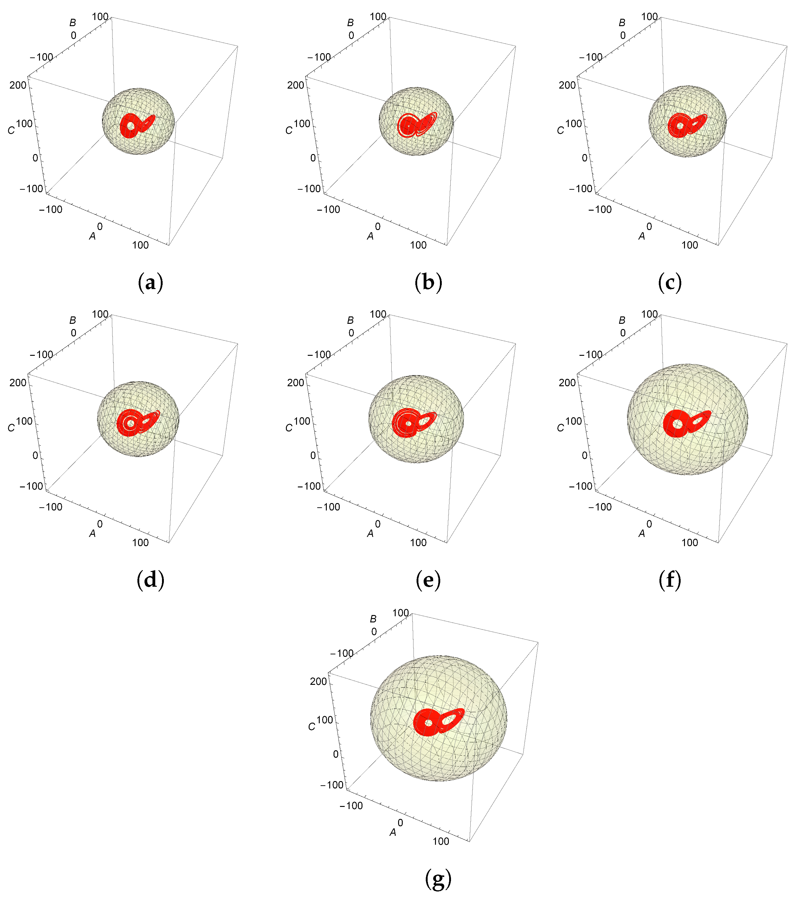
5.3. Ellipsoidal Bound on the Solution (Trajectory)

We now show that there is a bounded ellipsoid, E, within which all trajectories of the generalized Lorenz system (67)–(69) remain. In order to show this aspect, we multiply Equations (67)–(69) by A, B, and $C-\mathcal{C}$, respectively, where $\mathcal{C}=(c_{12}{Pr}^{*}+c_{21}R{a}^{*})/c_{32}$. Adding the resultant equations and rearranging them, we obtain

$$\begin{array}{c}\hfill {\displaystyle \frac{d\mathcal{L}}{d\tau }}=-\left[c_{11}{Pr}^{*}{A}^2+c_{22}{B}^2+b^{*}{c}_{31}{\left(C-{\displaystyle \frac{\mathcal{C}}{2}}\right)}^2-b^{*}{c}_{31}{\displaystyle \frac{{\mathcal{C}}^2}{4}}\right],\end{array}$$

(72)

where $\mathcal{L}={\displaystyle \frac{1}{2}}[A^2+B^2+{(C-\mathcal{C})}^2]$.

The quantity $\mathcal{L}$ is a Lyapunov function if the trajectory of $(A,B,C)$ remains bounded within the ellipsoid:

$$\begin{array}{c}\hfill {\displaystyle \frac{A^2}{{\mathtt{a}}^2}}+{\displaystyle \frac{B^2}{{\mathtt{b}}^2}}+{\displaystyle \frac{C^2}{{\mathtt{c}}^2}}=1,\end{array}$$

(73)

where

$$\begin{array}{c}\hfill \mathtt{a}=\sqrt{{\displaystyle \frac{c_{31}{b}^{*}}{c_{11}{Pr}^{*}}}}\left({\displaystyle \frac{\mathcal{C}}{2}}\right),\mathtt{b}=\sqrt{{\displaystyle \frac{c_{31}{b}^{*}}{c_{22}}}}\left({\displaystyle \frac{\mathcal{C}}{2}}\right),\mathtt{c}={\displaystyle \frac{\mathcal{C}}{2}}.\end{array}$$

5.4. Energy-Conserving Nature of the System

To prove that the generalized Lorenz system (67)–(69) is energy-conserving within the dissipationless limit, we consider the kinetic energy, $\mathcal{T}$, and the potential energy, $\mathcal{V}$, as given below:

$$\begin{array}{c}\hfill \mathcal{T}={\displaystyle \frac{1}{2}}[u^2+v^2],\mathcal{V}=-\frac{R{a}^{*}{Pr}^{*}}{2}\left({\mathsf{\Theta }}_1^2+{\mathsf{\Theta }}_2^2\right),\end{array}$$

(74)

where

$${\mathsf{\Theta }}_1=B\left(t\right)cos\left(\pi ax\right)G\left(y\right)\mathrm{and}{\mathsf{\Theta }}_2=C\left(t\right)F^{\prime }\left(y\right)G\left(y\right).$$

Using the perturbed version of Equation (16), we can write the kinetic energy in terms of the stream function as

$$\mathcal{T}=\frac{1}{2}\left[{\left(\frac{\partial \mathsf{\Psi }}{\partial x}\right)}^2+{\left(-\frac{\partial \mathsf{\Psi }}{\partial y}\right)}^2\right].$$

(75)

Substituting Equation (62) into (75), and simplifying and integrating over one Bénard cell, we obtain the total kinetic energy, $\mathcal{T}$, in the form

$$\mathcal{T}=-{\displaystyle \frac{{\delta }^4}{{\pi }^4{\alpha }^3}}\left[F(F^{\prime \prime }-{\pi }^2{\alpha }^{2}F)\right]A^2$$

(76)

Now, substituting ${\mathsf{\Theta }}_1$ and ${\mathsf{\Theta }}_2$ into (74), simplifying and integrating over one Bénard cell, we obtain the total potential energy, $\mathcal{V}$, in the form

$$\mathcal{V}={\displaystyle \frac{{Pr}^{*}R{a}^{*}}{2{\pi }^2}}\left[{\displaystyle \frac{2}{\alpha }}<G,G>B^2-<G,F{F}^{\prime \prime }G>C^2\right].$$

(77)

The total energy, $E\left(\tau \right)$, is given by

$$E\left(\tau \right)=\mathcal{T}+\mathcal{V}.$$

(78)

Substituting $\mathcal{T}$ and $\mathcal{V}$ from Equations (76) and (77) into Equation (78), and then differentiating with respect to $\tau$, we obtain a simplification

$$\begin{array}{ccc}\hfill \frac{d}{d\tau }E\left(\tau \right)& =& -\frac{{\delta }^6{\left({Pr}^{*}\right)}^2}{2{\pi }^4{\alpha }^3}\left[\left({\displaystyle \frac{c_{11}}{c_{12}}}\right)<F,G>(A^2+R{a}^{*}{B}^2)\right.\hfill \\ & & +{\displaystyle \frac{b^{*}\alpha c_{31}}{2}}<F^{\prime }G,F^{\prime }G>C^2\hfill \\ & & +{\displaystyle \frac{1}{\pi R{a}^{*}}}\left(1-{\displaystyle \frac{\alpha }{2{\delta }^2}}\right)<FG,F^{\prime }{G}^{\prime }>ABC\hfill \\ & & \left.+{\displaystyle \frac{1}{\pi R{a}^{*}}}\left(1+{\displaystyle \frac{\alpha }{2{\delta }^2}}\right)<FG,F^{\prime }G>ABC\right].\hfill \end{array}$$

(79)

From Equation (79), in the dissipationless limit, viz., ${Pr}^{*}\to 0$, we obtain

$$\frac{d}{dt}E\left(t\right)=0.$$

(80)

Equation (80) is a statement of the conservation of energy. In view of this, we conclude that the generalized Lorenz model of (67)–(69) is energy conserving within the dissipationless limit.

By considering the aforementioned nature of the symmetry, as dissipative, and the existence of the bounding ellipsoid and energy-conserving properties, we conclude that the generalized Lorenz model (67)–(69) has properties seen in the classical Lorenz model [42]. Hence, it is natural to anticipate chaotic behavior in the system (67)–(69) when $R{a}^{*}$ greatly exceeds $R{a}_c^{*}$. We next determine the threshold eigenvalue at which the chaotic attractor manifests.

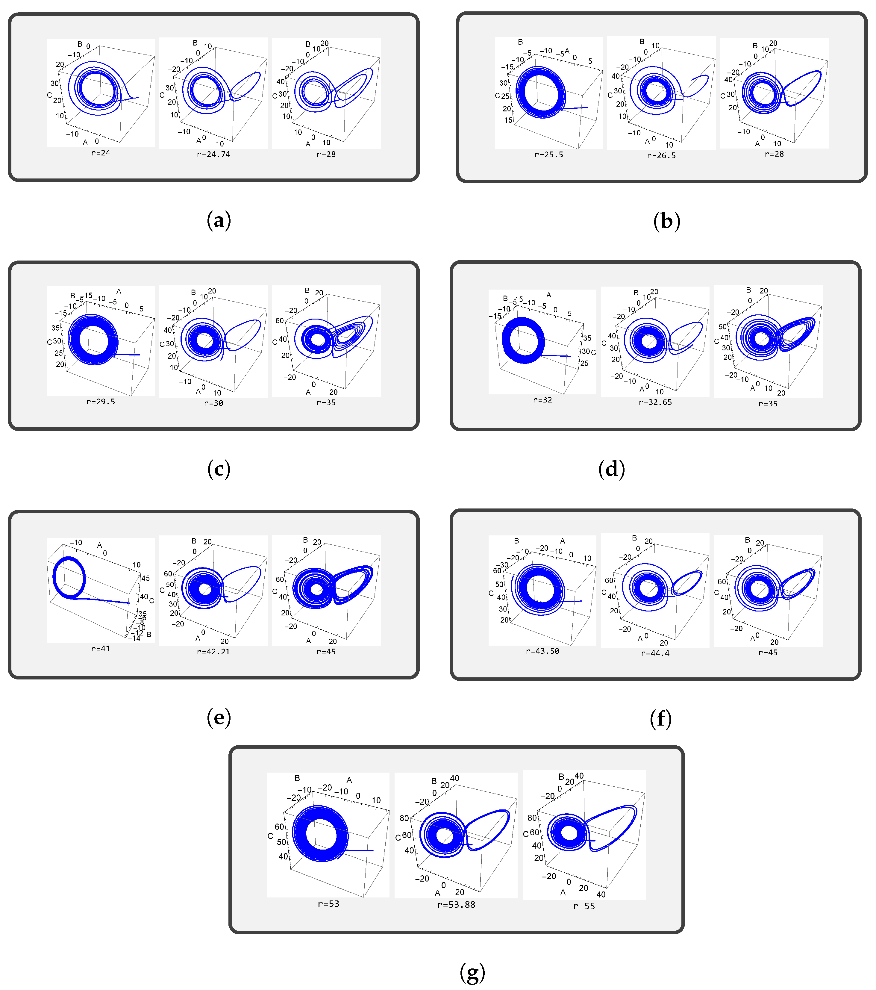
5.5. Prediction of the Onset of Chaos Using the Generalized Lorenz Model

The critical points of the generalized Lorenz model of (67)–(69) are given by

$$\begin{array}{c}\hfill \left.\begin{array}{c}\hfill (0,0,0),\left(q_1,\left({\displaystyle \frac{c_{11}}{c_{12}R{a}^{*}}}\right)q_1,\left({\displaystyle \frac{c_{11}{c}_{32}}{2b^{*}{c}_{12}{c}_{31}R{a}^{*}}}\right)q_1^2\right),\\ \hfill \left(-q_1,-\left({\displaystyle \frac{c_{11}}{c_{12}R{a}^{*}}}\right)q_1,\left({\displaystyle \frac{c_{11}{c}_{32}}{2b^{*}{c}_{12}{c}_{31}R{a}^{*}}}\right)q_1^2\right),\end{array}\right\},\end{array}$$

where $q_1=\sqrt{\frac{2b^{*}{c}_{31}\left(c_{12}{c}_{21}R{a}^{*}-c_{11}{c}_{22}\right)}{c_{11}{c}_{23}{c}_{32}}}$.

Among the three critical points noted above, $(0,0,0)$ corresponds to the pre-onset and the other two are post-onset points. We shall now linearize the Lorenz model about one post-onset critical point, say $\left(q_1,\left({\displaystyle \frac{c_{11}}{c_{12}R{a}^{*}}}\right)q_1,\left({\displaystyle \frac{c_{11}{c}_{32}}{2b^{*}{c}_{12}{c}_{31}R{a}^{*}}}\right)q_1^2\right)$.

Let

$$\begin{array}{c}\hfill \left.\begin{array}{c}A=q_1+\tilde{A},B=\left({\displaystyle \frac{c_{11}}{c_{12}R{a}^{*}}}\right)q_1+\tilde{B},\hfill \\ C=\left({\displaystyle \frac{c_{11}{c}_{32}}{2b^{*}{c}_{12}{c}_{31}R{a}^{*}}}\right)q_1^2+\tilde{C}\hfill \end{array}\right\}.\end{array}$$

(81)

The quantities $(\tilde{A},\tilde{B},\tilde{C})$ are slight deviations from the critical point. The product of these deviations is negligibly small. Using the above decomposition in the system (67)–(69) and neglecting the products of quantities with ~ we obtain the linearized Lorenz model in the form

$$\begin{array}{c}\hfill {\displaystyle \frac{d\mathcal{X}}{dt}}=\mathcal{A}\mathcal{X},\end{array}$$

(82)

where $\mathcal{X}={[\tilde{A},\tilde{B},\tilde{C}]}^{Tr}$ and

$$\begin{array}{c}\hfill \mathcal{A}=\left[\begin{array}{ccc}-c_{11}P{r}^{*}& c_{12}P{r}^{*}R{a}^{*}& 0\\ c_{21}-\left({\displaystyle \frac{c_{11}{c}_{23}{c}_{32}}{2c_{12}{c}_{31}R{a}^{*}}}\right)q_1^2& -c_{22}& -c_{23}{q}_1\\ \left({\displaystyle \frac{c_{11}{c}_{32}}{2c_{12}R{a}^{*}}}\right)q_1& {\displaystyle \frac{c_{32}}{2}}{q}_1& -c_{31}\end{array}\right].\end{array}$$

The auxiliary equation associated with the above equation is given by

$$|\mathcal{A}-\lambda I|=0,$$

where $\lambda$ is the characteristic root and I is the $3\times 3$ identity matrix.

On expansion of the determinant, we obtain

$$f\left(\lambda \right)=-{\lambda }^3-s_2{\lambda }^2-s_1\lambda +s_0=0,$$

(83)

where the coefficients are given by

$$\begin{array}{ccc}\hfill s_2& =& c_{11}{Pr}^{*}+c_{22}+c_{31},\hfill \\ \hfill s_1& =& c_{11}{c}_{31}{Pr}^{*}+{\displaystyle \frac{c_{12}{c}_{21}{c}_{31}R{a}^{*}}{c_{11}}},\hfill \\ \hfill s_0& =& 2c_{31}{Pr}^{*}\left(c_{11}{c}_{22}-c_{12}{c}_{21}R{a}^{*}\right).\hfill \end{array}$$

The roots of Equation (83) are real if

$$R{a}^{*}=\left(c_{11}{c}_{22}\right)/\left(c_{12}{c}_{21}\right).$$

When $R{a}^{*}>\left(c_{11}{c}_{22}\right)/\left(c_{12}{c}_{21}\right)$ we have one real root and a pair of complex conjugate roots. When we increase $R{a}^{*}$ further, say $R{a}_H^{*}$, these complex conjugate roots cross the complex plane’s imaginary axis, leading to a Hopf bifurcation. To find $R{a}_H^{*}$, we replace $\lambda$ with $i\lambda$ in Equation (83) and equate to zero the real and imaginary parts of the resulting equations, to obtain two expressions for ${\lambda }^2$. Equating the two expressions of ${\lambda }^2$ and simplifying, we obtain the modified Hopf–Rayleigh number $R{a}_H^{*}$ as:

$$r_H=\widetilde{Pr}\left({\displaystyle \frac{\widetilde{Pr}+\tilde{b}+3}{\widetilde{Pr}-\tilde{b}-1}}\right),$$

(84)

where

$$\begin{array}{c}\hfill \left.\begin{array}{c}\hfill r_H=R{a}_H^{*}/R{a}_c^{*},R{a}_c^{*}=\left(c_{11}{c}_{22}\right)/\left(c_{12}{c}_{21}\right),\\ \hfill \widetilde{Pr}=(c_{11}/c_{22})P{r}^{*}\mathrm{and}\tilde{b}=(c_{31}/c_{22})b^{*}\end{array}\right\}.\end{array}$$

6. Results and Discussion

This work concerning Brinkman–Bénard convection with general boundary conditions for velocity and temperature is reported to show that it is possible to unify various problems that have the same governing equations but different boundary conditions. To be precise, the 36 different problems covered by this study are

• Brinkman–Bénard convection problem with 16 different boundary conditions;
• Rayleigh–Bénard convection problem with 16 different boundary conditions (see, Table 2 for a list of these conditions);
• Darcy–Bénard convection problem with 4 different temperature boundary conditions.

Since the focus of this work is on covering many related problems in an integrated manner, we will not digress here to discuss individual boundary conditions and whether they are of practical utility or not.

Before we move on to a discussion of the results of both linear and nonlinear theories, we make brief mention of the choice of parameter values. The parameters appearing in the study are $Pr$, $\mathsf{\Lambda }$, ${\sigma }^2$, $S_l$, $S_u$, $B{i}_l$, $B{i}_u$, and $\lambda$. Apart from these, we also have the non-dimensional quantity of porosity, $\varphi$. The product of $Pr$, $\lambda$, and $\varphi$ appears together and hence we have called this product $P{r}^{*}$ and assigned a value of 10, which is much higher than that of water. To cover the extreme cases of free and rigid boundaries, as well as a rough boundary, it is essential that we take the entire range of values from zero to infinity. For computation, zero is taken to be a very small positive value, ${10}^{-3}$, and infinity is taken to be a very large positive value, ${10}^{+6}$. This decision about zero and infinity was taken through the observation of computational values in very general and limiting cases. The same reasoning was applied when choosing the range of values of $B{i}_l$ and $B{i}_u$ for zero to infinity.

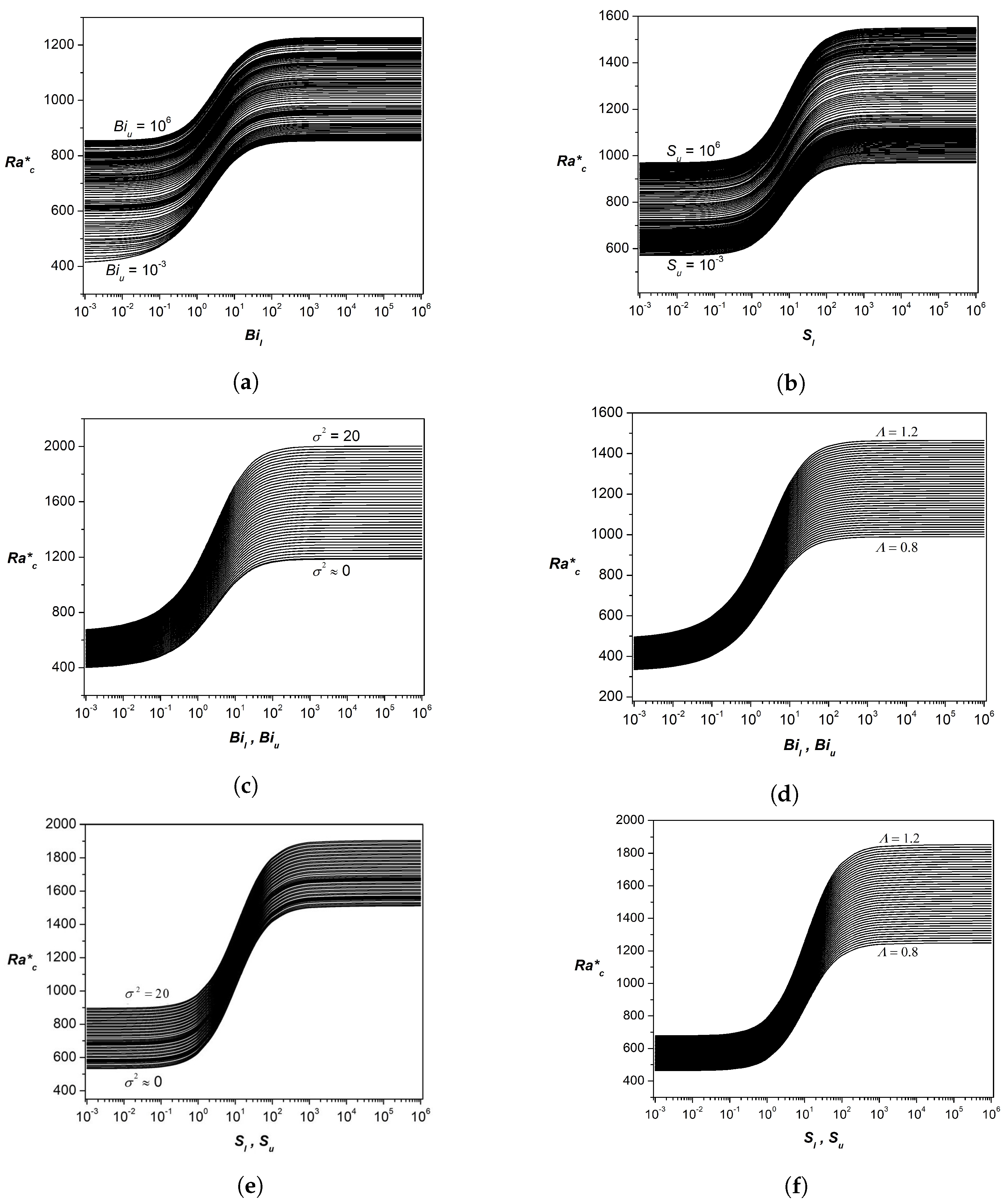
6.1. Discussion of the Results from Linear Theory

The critical Rayleigh number corresponding to marginal stationary stability was found using the eigenvalue of the BEVP of Equations (31) and (32), subject to general boundary conditions. Variation of the critical Rayleigh number and the critical wave number with non-dimensional parameters is presented in Table 3, as well as in Figure 2 and Figure 3. A very small slip Darcy number indicates a stress-free boundary condition, and a very large slip Darcy number indicates a rigid boundary condition. Moderate values indicate a rough boundary condition.

Figure 2. Variation of the critical Rayleigh number, $R{a}_c^{*}$, with various parameters. (a) Isothermal to adiabatic. (b) Free to rigid. (c) Clear liquid to densely packed medium, and isothermal to adiabatic. (d) Effect of viscosity ratio, and isothermal to adiabatic. (e) Clear liquid to densely packed medium, and free to rigid. (f) Effect of viscosity ratio, and free to rigid.

Figure 3. Variation of the critical wave number, $a_c$, with various parameters. (a) Isothermal to adiabatic. (b) Free to rigid. (c) Clear liquid to densely packed medium, and isothermal to adiabatic. (d) Effect of viscosity ratio, and isothermal to adiabatic. (e) Clear liquid to densely packed medium, and free to rigid. (f) Effect of viscosity ratio, and free to rigid.

The Biot number characterizes the relative difference between the thermal resistance inside the layer and at the boundary surface. If the Biot number is very small, this indicates that the thermal resistance at the boundary surface exceeds the thermal resistance inside the layer, and this is the case for a thermally insulated boundary condition. For this type of boundary condition, all the supplied energy can develop instability, and hence the onset occurs much earlier than in the case when the Biot number has finite or infinite values. The critical wave number is equal to zero (large cell), as a result of all the accumulated thermal energy being used for cell formation. In the case of both boundaries being adiabatic, an asymptotic analysis is performed to arrive at the expression of the critical Rayleigh number, by assuming a very small wave number for the regular perturbation expansion. From the expression (61), one can obtain the results of $FAFA$, $RARA$, and $RAFA\left(FARA\right)$, and these coincide with the classical results. Finite values of $B{i}_u$ and $B{i}_l$ yield a critical Rayleigh number and a critical wave number, in respect of bounding plates with an arbitrarily low heat conductivity. On the other hand, if the thermal resistance of the bounding surface is much less than the thermal resistance inside the layer, then this is a case of an isothermal boundary condition or a perfect conductor. The larger the value of the Biot number, the larger the critical Rayleigh number, meaning that larger Biot number systems are most stable. When this boundary condition is imposed, there is no heat flux across the boundary. This implies that the thermal fluctuation relaxes infinitely rapidly.

The inverse Darcy number, ${\sigma }^2$, characterizes the extent of occupation of the solid phase in the liquid medium within the sandwiched porous region. A small value of ${\sigma }^2$ would mean that the porous medium is sparsely packed, while a large value would mean it is densely packed. The slip Darcy numbers $S_l$ and $S_u$ arise due to the application of the Beavers–Joseph slip condition at the interface between the sandwiched porous medium and its bounding porous walls, which are densely packed. The porous interface renders the surface rough. The two rough porous walls are considered to be dissimilar, in the sense that they have unequal yet constant values of thermal resistance and permeability. The effective viscosity ratio, $\mathsf{\Lambda }$, in the two porous walls was assumed to be the same, to keep the number of parameters as low as possible. From earlier experience on porous-medium Bénard problems, it is evident that the effect of $\mathsf{\Lambda }$ on instability is comparatively small, in relation to the influence of other parameters. Keeping the parameter values in the two bounding porous walls unequal, we have the distinct advantage of extracting results for a maximum number of limiting cases from our study.

In Figure 2 and Figure 3, we present the influence of all parameters on $R{a}_c^{*}$ and $a_c$, respectively. In presenting the effect of the variation of a particular parameter on $R{a}_c^{*}$ and $a_c$, we consider moderate values of the other fixed parameters. This procedure was adopted after ascertaining computationally that the scenario remained similar at values other than moderate values. In Figure 2a, the extreme values of $B{i}_l$ and $B{i}_u$ (from very small to very large) refer to insulated and isothermal boundary conditions, respectively. Intermediate values refer to situations in which the thermal resistance at the boundary surface either exceeds or is in deficit of the thermal resistance inside the layer. Thus, it is obvious from the linear stability analysis with general boundary conditions that we were able to bridge the gap between the results of insulated and isothermal boundary conditions at the two bounding surfaces. Figure 2b illustrates a similar situation as that in Figure 2a for the case of shear matching at the interfaces. The gap in the results between the free boundary and rigid boundary conditions at the interfaces were bridged. An extremely small value of $S_l$ and $S_u$ indicates a free boundary and an extremely large value suggests a rigid boundary. Intermediate values indicate results pertaining to a rough boundary condition. The results of Figure 2c–f are essentially a reiteration of the earlier results for different values of ${\sigma }^2$ and $\mathsf{\Lambda }$. The intention behind the presentation of the results in Figure 3 is identical to that expressed in the context of Figure 2. Table 3 has been included for completeness, though it is only a tabulated result of the pictorial representation in Figure 2 and Figure 3. To increase confidence in the results obtained, we validated the results of the present study by comparing the results in several limiting cases. Table 2 and Table 4 document these results and indicate that we achieved this objective. In what follows, we discuss the results of the weakly nonlinear stability analysis.

Table 4. Values of the critical Darcy–Rayleigh number $R{a}_c^{*}$ and the wave number ${\alpha }_c=\pi a_c$ for different boundary conditions, taking $\mathsf{\Lambda }=0$ and ${\sigma }^2=1$.

Type of Boundaries	Present Study		Nield and Bejan [8]
	${\mathit{\alpha }}_{\mathit{c}}$	${\mathit{Ra}}_{\mathit{c}}^{*}$	${\mathit{\alpha }}_{\mathit{c}}$	${\mathit{Ra}}_{\mathit{c}}^{*}$
Isothermal–Isothermal	3.1416	39.4783	3.14	39.48
Isothermal–Adiabatic	2.3263	27.0976	2.33	27.10
Adiabatic–Isothermal	2.3263	27.0976	-	-
Adiabatic–Adiabatic	0.005	12.0013	0	12

6.2. Discussion of Results Using Nonlinear Stability Theory

Before providing a discussion of the results of the nonlinear analysis, we now make some general remarks. We note that the structure of the Lorenz model (67)–(69) is the same as that of the classical Lorenz model [42], with the coefficients being different. We call the Lorenz model of this paper a generalized Lorenz model. The values of the parameters considered in the nonlinear analysis for the purpose of computation were the same as those chosen in the linear analysis. The intention behind the choice was the same in the two analyses. In view of the innumerable number of possible limiting cases, we considered only a few representative cases.

Table 5 and Table 6 document the coefficients of the generalized Lorenz model for different combinations of parameter values. The tabulated values are included to note the fact that the various quantities characterizing the model were all within a certain expected range of values. This lends credence to the procedure adopted in the paper for arriving at a generalized Lorenz model. The last three columns, viz., $\tilde{b}$, $\widetilde{Pr}$, and $r_H$, are scaled versions of the counterparts of the corresponding quantities of the classical Lorenz model [42]. We observe that these values are within the expected range. There are exceptions, however, in the cases when $B{i}_l$ and $B{i}_u$ are very small, which are the cases of adiabatic boundaries. Knowing that such boundaries are not physically realistic, one may consider, without any doubt, the obtained values of $\tilde{b}$, $\widetilde{Pr}$, and $r_H$ as acceptable values. As a consequence of this observation, we deliberately refrained from making any further calculations pertaining to boundaries where both are adiabatic.

Table 5. Coefficients of the Lorenz system and the Hopf–Rayleigh number for different values of lower and upper slip Darcy numbers with $\mathsf{\Lambda }=1$, ${\sigma }^2=1$ and $B{i}_l=B{i}_u=10$.

${\mathit{S}}_{\mathit{l}}$	${\mathit{S}}_{\mathit{u}}$	Coefficients of the Lorenz System						$\tilde{\mathit{b}}$	$\widetilde{\mathit{Pr}}$	${\mathit{r}}_{\mathit{H}}$
		${\mathit{c}}_{\mathbf{11}}$	${\mathit{c}}_{\mathbf{12}}={\mathit{c}}_{\mathbf{21}}$	${\mathit{c}}_{\mathbf{22}}$	${\mathit{c}}_{\mathbf{23}}$	${\mathit{c}}_{\mathbf{31}}$	${\mathit{c}}_{\mathbf{32}}$
${10}^{-3}$	10	21.8455	0.0275630	12.7768	1.0473500	31.3206	1.6084	2.45136	17.0977	28.2521
${10}^{-2}$		21.8623	0.0275663	12.7798	1.0498800	31.3238	1.60835	2.45104	17.1070	28.2587
${10}^{-1}$		22.0362	0.0276072	12.8116	1.0750500	31.3630	1.60815	2.44802	17.2002	28.3267
0.4		22.5837	0.0277281	12.9102	1.1609500	31.4934	1.60733	2.43942	17.4930	28.5448
0.6		22.9231	0.0277962	12.9707	1.2199800	31.5795	1.60669	2.43468	17.6729	28.6818
1		23.5490	0.0279101	13.0823	1.3422100	31.7525	1.60546	2.42713	18.0006	28.9371
2		24.8594	0.0280961	13.3122	0.4181370	32.1667	1.60212	2.41633	18.6742	29.4845
3		25.8944	0.0281910	13.4922	0.2265190	32.5472	1.59884	2.41230	19.1922	29.9251
4		26.7298	0.0282318	13.6361	0.1525550	32.8891	1.59569	2.41192	19.6023	30.2857
5		27.4177	0.0282411	13.7542	0.1151720	33.1956	1.59281	2.41349	19.9341	30.5850
10		29.5728	0.0281073	14.1238	0.0561866	34.3103	1.58172	2.42925	20.9382	31.5317
${10}^2$		33.3935	0.0270043	14.8052	0.0211920	37.0307	1.55216	2.50119	22.5552	33.2118
${10}^3$		33.9318	0.0266963	14.9104	0.0186483	37.5320	1.54639	2.51717	22.7572	33.4430
${10}^6$		33.9923	0.0266573	14.9228	0.0183795	37.5915	1.5457	2.51906	22.7787	33.4682
10	${10}^{-3}$	21.8446	0.0275619	12.7768	0.0620477	31.3201	1.60838	2.45132	17.0971	28.2514
	${10}^{-2}$	21.8621	0.0275660	12.7799	0.0620323	31.3237	1.60834	2.45101	17.1067	28.2584
	${10}^{-1}$	22.0362	0.0276073	12.8115	0.0618777	31.3627	1.60813	2.44802	17.2004	28.3269
	0.4	22.5836	0.0277279	12.9101	0.0613983	31.4930	1.60731	2.43942	17.4930	28.5448
	0.6	22.9229	0.0277961	12.9709	0.0611065	31.5799	1.60671	2.43467	17.6726	28.6815
	1	23.5491	0.0279102	13.0821	0.0605773	31.7522	1.60544	2.42714	18.0009	28.9374
	2	24.8593	0.0280959	13.3124	0.0595116	32.1669	1.60213	2.41632	18.6738	29.4842
	3	25.8944	0.0281910	13.4922	0.0587126	32.5471	1.59884	2.41230	19.1922	29.9251
	4	26.7302	0.0282322	13.6361	0.0580950	32.8894	1.59571	2.41194	19.6025	30.2859
	5	27.4179	0.0282413	13.7542	0.0576061	33.1957	1.59281	2.41350	19.9343	30.5851
	10	29.5728	0.0281073	14.1238	0.0561866	34.3103	1.58172	2.42925	20.9382	31.5317
	${10}^2$	33.3923	0.0270033	14.8052	0.0540763	37.0301	1.55214	2.50116	22.5544	33.2110
	${10}^3$	33.9316	0.0266961	14.9103	0.0538163	37.5318	1.54638	2.51718	22.7572	33.4430
	${10}^6$	33.9926	0.0266569	14.9224	0.0537878	37.5915	1.54566	2.51913	22.7795	33.4692
${10}^{-3}$	${10}^{-3}$	15.3800	0.0269441	11.4402	1.0373900	28.3338	1.64971	2.47669	13.4439	25.5203
${10}^{-2}$	${10}^{-2}$	15.4116	0.0269554	11.4470	1.0401700	28.3428	1.64962	2.47599	13.4634	25.5310
${10}^{-1}$	${10}^{-1}$	15.7209	0.0270617	11.5131	1.0681100	28.4282	1.64851	2.46919	13.6548	25.6376
0.4	0.4	16.6918	0.0273614	11.7176	1.1625000	28.7082	1.64479	2.45000	14.2450	25.9894
0.6	0.6	17.2938	0.0275248	11.8422	1.2265100	28.8921	1.64245	2.43976	14.6036	26.2190
1	1	18.4023	0.0277823	12.0675	1.3575300	29.2502	1.63793	2.42388	15.2495	26.6590
2	2	20.7339	0.0281668	12.5258	0.4260500	30.0877	1.62784	2.40206	16.5529	27.6346
3	3	22.5984	0.0283393	12.8788	0.2311810	30.8385	1.61908	2.39451	17.5469	28.4440
4	4	24.1284	0.0284021	13.1613	0.1555150	31.5103	1.61156	2.39415	18.3328	29.1179
5	5	25.4075	0.0284038	13.3928	0.1171170	32.1097	1.60497	2.39752	18.9709	29.6847
10	10	29.5728	0.0281073	14.1239	0.0561862	34.3106	1.58174	2.42926	20.9381	31.5316
${10}^2$	${10}^2$	37.8708	0.0260191	15.5322	0.0197446	40.0625	1.52524	2.57933	24.3822	35.1167
${10}^3$	${10}^3$	39.1744	0.0254341	15.7582	0.0170888	41.2115	1.51432	2.61524	24.8597	35.6609
${10}^6$	${10}^6$	39.3268	0.0253604	15.7849	0.0168051	41.3522	1.51302	2.61972	24.9142	35.7242

Table 6. Coefficients of Lorenz system and Hopf–Rayleigh number for different values of lower and upper Biot numbers with $\mathsf{\Lambda }=1$, ${\sigma }^2=1$, and $S_l=S_u=10$.

${\mathit{Bi}}_{\mathit{l}}$	${\mathit{Bi}}_{\mathit{u}}$	Coefficients of Lorenz System						$\tilde{\mathit{b}}$	$\widetilde{\mathit{Pr}}$	${\mathit{r}}_{\mathit{H}}$
		${\mathit{c}}_{\mathbf{11}}$	${\mathit{c}}_{\mathbf{12}}={\mathit{c}}_{\mathbf{21}}$	${\mathit{c}}_{\mathbf{22}}$	${\mathit{c}}_{\mathbf{23}}$	${\mathit{c}}_{\mathbf{31}}$	${\mathit{c}}_{\mathbf{32}}$
${10}^{-3}$	10	29.1037	0.0372074	7.20571	0.0366865	31.0650	1.20452	4.31117	40.3898	54.9233
${10}^{-2}$		29.1028	0.0371515	7.23585	0.0367666	31.0602	1.20599	4.29255	40.2203	54.7124
${10}^{-1}$		29.1179	0.0366544	7.52711	0.037520	31.0242	1.22037	4.12166	38.6841	52.7957
0.4		29.1582	0.0353018	8.36365	0.0396794	30.9802	1.26256	3.70415	34.863	48.0508
0.6		29.1850	0.0345965	8.83169	0.0408873	30.9989	1.28675	3.50996	33.0457	45.8073
1		29.2341	0.0334898	9.61121	0.0429139	31.1066	1.32794	3.23649	30.4167	42.5844
2		29.3284	0.0317191	10.9737	0.0465625	31.5566	1.40233	2.87565	26.726	38.1312
3		29.3946	0.0306572	11.8568	0.0490450	32.0571	1.45194	2.70369	24.7913	35.8509
4		29.4409	0.0299412	12.4751	0.0508662	32.5204	1.48711	2.60681	23.5997	34.4755
5		29.4782	0.0294267	12.9320	0.0522604	32.9310	1.51330	2.54648	22.7949	33.5632
10		29.5728	0.0281073	14.1238	0.0561866	34.3103	1.58172	2.42925	20.9382	31.5317
${10}^2$		29.7030	0.0263954	15.6651	0.0621767	36.9439	1.66819	2.35836	18.9613	29.5542
${10}^3$		29.7194	0.0261822	15.8504	0.0630031	37.3445	1.67818	2.35605	18.7499	29.3613
${10}^6$		29.7201	0.0261570	15.8709	0.0631004	37.3894	1.67922	2.35585	18.7262	29.3399
10	${10}^{-3}$	29.1030	0.0372064	7.20560	0.0486803	31.0649	1.20451	4.31121	40.3894	54.9230
	${10}^{-2}$	29.1039	0.0371528	7.23609	0.0487350	31.0599	1.20600	4.29236	40.2204	54.7120
	${10}^{-1}$	29.1165	0.0366526	7.52707	0.0492362	31.0239	1.22036	4.12165	38.6824	52.7941
	0.4	29.1589	0.0353027	8.36374	0.0505528	30.9811	1.26257	3.70421	34.8635	48.0514
	0.6	29.1843	0.0345957	8.83163	0.0512204	30.9977	1.28674	3.50986	33.0452	45.8065
	1	29.2338	0.0334894	9.61128	0.0522272	31.1063	1.32794	3.23643	30.4161	42.5837
	2	29.3288	0.0317196	10.9737	0.0537338	31.5570	1.40235	2.8757	26.7265	38.1318
	3	29.3944	0.0306570	11.8567	0.0545607	32.0570	1.45192	2.70371	24.7914	35.8511
	4	29.4414	0.0299416	12.4752	0.0550759	32.5205	1.48711	2.60681	23.5999	34.4757
	5	29.4781	0.0294266	12.9320	0.0554203	32.9312	1.51331	2.54650	22.7947	33.5631
	10	29.5728	0.0281073	14.1238	0.0561866	34.3103	1.58172	2.42925	20.9382	31.5317
	${10}^2$	29.7029	0.0263953	15.6650	0.0568236	36.9433	1.66817	2.35834	18.9614	29.5542
	${10}^3$	29.7186	0.0261815	15.8503	0.0568663	37.3437	1.67815	2.35602	18.7495	29.3609
	${10}^6$	29.7201	0.0261570	15.8709	0.0568710	37.3895	1.67923	2.35585	18.7261	29.3399
${10}^{-3}$	${10}^{-3}$	29.9469	0.0721017	0.18038	0.0075992	29.0540	1.00387	161.073	1660.23	2021.65
${10}^{-2}$	${10}^{-2}$	29.7094	0.0682501	0.57548	0.0133728	29.0095	1.01288	50.4096	516.258	632.670
${10}^{-1}$	${10}^{-1}$	29.2270	0.0584225	1.86821	0.0231062	28.8743	1.04692	15.4556	156.444	195.459
0.4	0.4	28.9703	0.0485894	3.83446	0.0315834	28.7699	1.10935	7.50299	75.5525	96.9687
0.6	0.6	28.9491	0.0453658	4.72113	0.0344888	28.7900	1.1409	6.09812	61.3181	79.6347
1	1	28.9757	0.0413102	6.09413	0.0384156	28.9332	1.19337	4.74772	47.5469	62.8980
2	2	29.1104	0.0361915	8.40381	0.0440987	29.5681	1.29092	3.51841	34.6395	47.3320
3	3	29.2262	0.0335830	9.92005	0.0474722	30.3189	1.36108	3.05633	29.4618	41.1891
4	4	29.3155	0.0319563	11.0126	0.0497992	31.0588	1.41469	2.82031	26.6201	37.8761
5	5	29.3841	0.0308321	11.8412	0.0515263	31.7464	1.45706	2.68101	24.8150	35.8077
10	10	29.5728	0.0281073	14.1238	0.0561866	34.3103	1.58172	2.42925	20.9382	31.5317
${10}^2$	${10}^2$	29.8318	0.0247867	17.4254	0.0629192	40.3437	1.78355	2.31523	17.1198	27.8229
${10}^3$	${10}^3$	29.8621	0.0243830	17.8561	0.0638208	41.4017	1.81174	2.31863	16.7237	27.4992
${10}^6$	${10}^6$	29.8672	0.0243384	17.9056	0.0639213	41.5289	1.81507	2.31932	16.6803	27.4651

Extensive computation of the solution to the generalized Lorenz model was performed, to cover all possible ranges of parameter values. For each combination of parameter values, the value of $r_H$ obtained analytically using Equation (84) was considered, to meticulously check the veracity of the prediction made using the bifurcation diagram. In all cases, there was a perfect match between the two values. We considered 12 boundary combinations out of the 16 possible ones, by omitting those boundaries which were both adiabatic. Out of the 12, some demonstrated the duplication of values with other cases (due to symmetry), and these five were bunched together in the bifurcation diagrams, phase space plots, and the Lyapunov spectrum. As a result, in Figure 4, Figure 5 and Figure 6, we only see plots of the seven boundary combinations whose results were different from each other. In these plots, we see only the results pertaining to a sandwiched clear liquid layer (no porous matrix, i.e., ${\sigma }^2=0)$. We ascertained that similar results were seen when ${\sigma }^2\ne 0$ (sandwiched porous-medium).

Figure 4. Bifurcation diagrams of the generalized Lorenz model for different boundary conditions using the initial conditions (1, 1, 1), $\mathsf{\Lambda }=1$, and ${\sigma }^2=0$. (a) FIFI. (b) FIRI (RIFI). (c) RIRI. (d) FAFI (FIFA). (e) FARI (RIFA). (f) FIRA (RAFI). (g) RARI (RIRA).

Figure 5. Phase space plots of the generalized Lorenz model for different boundary conditions using the initial conditions (1, 1, 1), $\mathsf{\Lambda }=1$, ${\sigma }^2=0$, and for different values of r. (a) FIFI. (b) FIRI (RIFI). (c) RIRI. (d) FAFI (FIFA). (e) FARI (RIFA). (f) FIRA (RAFI). (g) RARI (RIRA).

Figure 6. Ellipsoid and phase space plots of the generalized Lorenz model for different boundary conditions using the initial conditions (1, 1, 1), $r=55$, $\mathsf{\Lambda }=1$, and ${\sigma }^2=0$. (a) FIFI. (b) FIRI (RIFI). (c) RIRI. (d) FAFI (FIFA). (e) FARI (RIFA). (f) FIRA (RAFI). (g) RARI (RIRA).

The bifurcation diagrams in Figure 4 are plots made through considering the time series of $C\left(t\right)$ and extracting local maximum values from it. To find the time series of $C\left(t\right)$, numerical integration of the Lorenz system (67)–(69) using the standard fourth-order Runge–Kutta method, with a step-size of $\mathsf{\Delta }t={10}^{-5}$, was performed, and the local maximum of $C(t$) in the time interval (0, 1000) was extracted. The bifurcation diagram depicts the transition to chaos at the Hopf bifurcation point, $r=r_H$, and the chaotic motion seen beyond $r_H$ in the $C_{Max}-r$ plane was interrupted by periodic motions of various periodicities. The intensity of chaos in each period was determined using vigorous oscillations or otherwise, as seen in the diagram. The more vigorous the oscillations the more chaotic the system. A period of periodic motion serves the purpose of conserving energy (fueling zone), which is later used in the next spell of chaos for its sustenance in a range of values of r. From the bifurcation diagrams with respect to the various boundary combinations shown in Figure 4, it is clear that they look alike in content, except for the fact that they are translated versions of each other. In the case when one of the boundaries is adiabatic, the chaos is more intense compared to that in the case when both boundaries are isothermal. This is obviously due to the lack of exchange of thermal energy through such a boundary between the system and its surrounding. Now, coming to the aspects pertaining to the velocity boundary condition, it was found that, in the case of a rigid boundary combination, the appearance of chaos or periodic motion took place at large values of r, almost three times that in the case of the free boundary combination. We even noticed this result in the case of linear theory, due to the liquid sticking to the rigid boundary.

Figure 5 shows phase-space plots of the seven chosen boundary combinations. Three ranges of values of r are considered in each plot: $r<r_H$, $r=r_H$, and $r>r_H$. The phase-space plot pertaining to $r<r_H$ is typically that of regular convective motion. Looking at the plot for $r=r_H$, we obtain a picture of the trajectories moving away from one of the post-onset critical points and proceeding towards the other post-onset critical point. A very important point to note regarding these trajectories is that the nonlinear terms, $AB$ and $AC$, in the generalized Lorenz model are responsible for keeping the trajectories within the ellipsoidal trapping region. In other words, this means the solution to the generalized Lorenz model always remains bounded. Applying the Lipschitz condition to the initial value problem involving the generalized Lorenz model, it can be seen that the various loop-like structures (butterfly diagram) are non-intersecting. This is a case of chaotic dynamics. In the case when periodic motion appears beyond $r_H$, the trajectories traced the same loop(s). The number of loops, say n, seen in the phase space plots indicates that the periodic motion is of period n.

As in the case of the classical Lorenz model [42], in the generalized Lorenz model, one can also find a trapping region within which the trajectories remain (seen in Figure 3). This trapping region is an ellipsoid, as shown in Equation (73), and its volume depends on the boundary combination, as shown in Figure 6. Figure 7 is a justification for not considering the physically unrealistic boundary combinations of both boundaries as adiabatic. We have plotted the real part of the largest eigenvalue, ${\lambda }_1$, in the Lyapunov spectrum against r for the representative boundary combinations of $FAFA$. The figure clearly indicates the blowing up of Re(${\lambda }_2$) with r, thereby implying that this boundary combination is not viable. A similar observation holds good for $RARA$ and $RAFA\left(FARA\right)$.

Figure 7. The real part of the eigenvalue versus r. (a) FAFA. (b) Magnified plot of (a) around $r_H$.

At this point, we draw attention to an earlier work by [17], which covered all possible boundary combinations in the case of a clear liquid layer bounded by two surfaces. A Lorenz model of each case was derived using a single-term Galerkin procedure. On comparison of the corresponding values for $r_H$ from this paper with those of [17], it was found that the values of $r_H$ reported here are accurate values. This result is documented in Table 7. This table also indicates the confidence level for the results obtained using the Fourier–Galerkin single-term procedure. An important point also needs to be mentioned here: The method adopted here is also a single-term Fourier–Galerkin, but the trial function (polynomial with nearly 20 terms) is an accurate description of the eigenfunctions of the problem. This is the reason why one can have great confidence in the predicted results of this paper.

Table 7. Values of the Hopf–Rayleigh number for different boundary conditions, taking $\mathsf{\Lambda }=1$ and ${\sigma }^2=0$.

BC	FIFI	RIFI	FIRI	RIRI	FAFI	FIFA	FARI	RIFA	RAFI	FIRA	RARI	RIRA
Present study	24.74	26.20	26.20	30.00	32.64	32.64	42.21	42.21	44.37	44.37	53.87	53.87
Kanchana et al. [17]	24.74	29.13	27.09	35.28	43.38	51.00	43.08	42.46	46.97	45.52	45.35	63.03

We end the discussion of results with the observation that extensive computation revealed that the results obtained in the case of a sandwiched high porosity medium were qualitatively similar to those reported earlier for the case of a sandwiched clear liquid layer.

7. Summary

The overall conclusions drawn from this study are

(a)

It is possible to unify the study of linear and weakly nonlinear regimes of various related Rayleigh–Bénard problems with identical governing equations but different boundary conditions;

(b)

Using Maclaurin series representation, it is possible to have accurate representations for the eigenfunctions of both the conductive mode (linear theory) and convective modes (nonlinear theory);

(c)

The generalized Lorenz model has all the characteristics of the classical Lorenz model;

(d)

Classical linear and nonlinear stability analyses can be performed using the generalized Lorenz model, to obtain information on the onset of regular convection, chaos, and periodic motions;

(e)

The effect of increasing values of the Biot and slip Darcy numbers is to stabilize the system and decrease the cell size at the onset of regular convection;

(f)

The effect of increasing the values of the Biot and slip Darcy numbers on the onset of chaos is opposite;

(g)

The general velocity and thermal boundary conditions used in this paper succeeded in bridging the gap between the results of free and rigid boundaries, and also those of isothermal and adiabatic boundary conditions;

(h)

By analogy between the results of the present general study and its corresponding Taylor–Couette problem [43], the results of the linear theory for the latter problem are as good as known;

(i)

This analogy has been proven for linear theory, and further investigation is required to prove/disprove the analogy in the nonlinear regime.

References

- Muskat, M. The Flow of Fluids through Porous Media; McGraw Hill: New York, NY, USA, 1937. [Google Scholar]
- Scheidegger, M. The Physics of Flow through Porous Media; MacMillan: New York, NY, USA, 1957. [Google Scholar]
- Beck, J.L. Convection in a box of porous material saturated with fluid. Phys. Fluids 1972, 15, 1377–1383. [Google Scholar] [CrossRef]
- Vadasz, P. Free Convection in Rotating Porous Media: In Transport Phenomena in Porous Media; Elsevier: Pergamon, Turkey, 1998. [Google Scholar]
- Crolet, J.M. Computation Methods for Flow and Transport in Porous Media; Springer: Dordrecht, The Netherlands, 2000. [Google Scholar]
- Ingham, D.B.; Pop, I. Transport Phenomena in Porous Media; Elsevier: Oxford, UK, 2005. [Google Scholar]
- Vafai, K. Handbook of Porous Media; CRC Press: London, UK, 2005. [Google Scholar]
- Nield, D.A.; Bejan, A. Convection in Porous Media; Springer Science Business Media: New York, NY, USA, 2006. [Google Scholar]
- Straughan, B. The Energy Method, Stability, and Nonlinear Convection; Springer: New York, NY, USA, 2004. [Google Scholar]
- Straughan, B. Stability and Wave Motion in Porous Media; Springer: New York, NY, USA, 2008. [Google Scholar]
- Kaviany, M. Principles of Heat Transfer in Porous Media; Springer Science and Business Media: New York, NY, USA, 2012. [Google Scholar]
- Liu, S.; Jiang, L. From Rayleigh-Bénard convection to porous-media convection: How porosity affects heat transfer and flow structure. J. Fluid Mech. 2020, 895, A18. [Google Scholar] [CrossRef]
- Herring, J. Investigation of Problems in Thermal Convection: Rigid Boundaries. J. Atmos. Sci. 1964, 21, 277–290. [Google Scholar] [CrossRef]
- Kvernvold, O. Rayleigh-Bénard convection with one free and one rigid boundary. Geophys. Astrophys. Fluid Dyn. 1197, 92, 273–294. [Google Scholar] [CrossRef]
- Mizushima, J. Mechanism of mode selection in Rayleigh-Bénard convection with free-rigid boundaries. Fluid Dyn. Res. 1993, 11, 297–311. [Google Scholar] [CrossRef]
- Webber, M. The destabilizing effect of boundary slip on Bénard convection. Math. Methods Appl. Sci. 2006, 29, 819–838. [Google Scholar] [CrossRef]
- Kanchana, C.; Siddheshwar, P.G.; Yi, Z. The effect of boundary-conditions on the onset of chaos in Rayleigh-Bénard convection using energy-conserving Lorenz models. Appl. Math. Model. 2020, 88, 349–366. [Google Scholar] [CrossRef]
- Haragus, M.; Iooss, G. Domain Walls for the Bénard–Rayleigh Convection Problem with Rigid–Free boundary-conditions. J. Dyn. Differ. Equ. 2021, 34, 1–23. [Google Scholar] [CrossRef]
- Beavers, G.S.; Joseph, D.D. boundary-conditions at a naturally permeable wall. J. Fluid Mech. 1967, 30, 197–207. [Google Scholar] [CrossRef]
- Beavers, G.S.; Sparrow, E.M.; Masha, B.A. boundary-conditions at a porous surface which bounds a fluid flow. AIChE J. 1974, 20, 596–597. [Google Scholar] [CrossRef]
- Saffman, P.G. On the boundary-condition at the interface of a porous medium. Stud. Appl. Math. 1971, 1, 93–101. [Google Scholar] [CrossRef]
- Richardson, S. A model for the boundary-condition of a porous material Part 2. J. Fluid Mech. 1971, 49, 327–336. [Google Scholar] [CrossRef]
- Taylor, G.I. A model for the boundary-condition of a porous material, Part 1. J. Fluid Mech. 1971, 49, 319–326. [Google Scholar] [CrossRef]
- Goldstein, M.E.; Braun, W.H. Effect of Velocity Slip at a Porous Boundary on the Performance of an Incompressible Porous Bearing; NASA Technical Note; TN D-6181; NASA: Washington, DC, USA, 1971. [Google Scholar]
- Nield, D.A. Onset of convection in a fluid layer overlying a layer of a porous medium. J. Fluid Mech. 1977, 81, 513–522. [Google Scholar] [CrossRef]
- Pillatsis, G.; Taslim, M.E.; Narusawa, U. Thermal instability of a fluid saturated porous medium bounded by thin fluid layers. ASME J. Heat Mass Transf. 1987, 109, 677–682. [Google Scholar] [CrossRef]
- Givler, R.C.; Altobelli, S.A. A determination of the effective viscosity for the Brinkman–Forchheimer flow model. J. Fluid Mech. 1994, 258, 355–370. [Google Scholar] [CrossRef]
- Jäger, W.; Mikelic, A. On the interface boundary-condition of Beavers, Joseph and Saffman. SIAM J. Appl. Math. 2000, 60, 1111–1127. [Google Scholar]
- Barletta, A.; Storesletten, L. Onset of convection in a porous rectangular channel with external heat transfer to upper and lower fluid environments. Transp. Porous Media 2012, 94, 659–681. [Google Scholar] [CrossRef]
- Bolaños, S.J.; Vernescu, B. Derivation of the Navier slip and slip length for viscous flows over a rough boundary. Phys. Fluids 2017, 29, 057103. [Google Scholar] [CrossRef]
- Sahraoui, M.; Kaviany, M. Slip and no-slip velocity boundary-conditions at the interface of porous, plain media. Int. J. Heat Mass Transf. 1992, 35, 927–943. [Google Scholar] [CrossRef]
- Sahraoui, M.; Kaviany, M. Slip and no-slip temperature boundary-conditions at the interface of porous, plain media: Conduction. Int. J. Heat Mass Transf. 1993, 36, 1019–1033. [Google Scholar] [CrossRef]
- Sahraoui, M.; Kaviany, M. Slip and no-slip temperature boundary-conditions at the interface of porous, plain media: Convection. Int. J. Heat Mass Transf. 1994, 37, 1029–1044. [Google Scholar] [CrossRef]
- Siddheshwar, P.G. Convective instability of ferromagnetic fluids bounded by fluid-permeable, magnetic boundaries. J. Magn. Magn. Mater. 1995, 149, 148–150. [Google Scholar] [CrossRef]
- Narayana, M.; Shekar, M.; Siddheshwar, P.G.; Anuraj, N.V. On the differential transform method of solving boundary eigenvalue problems: An illustration. J. Appl. Math. Mech. Z. Für Angew. Math. Mech. 2021, 101, e202000114. [Google Scholar] [CrossRef]
- Heena, F.; Siddheshwar, P.G.; Idris, R. Effects of rough boundaries on Rayleigh–Bénard Convection in nanofluids. ASME J. Heat Mass Transf. 2023, 145, 062602. [Google Scholar]
- Celli, M.; Kuznetsov, A.V. A new hydrodynamic boundary-condition simulating the effect of rough boundaries on the onset of Rayleigh-Bénard convection. Int. J. Heat Mass Transf. 2018, 116, 581–586. [Google Scholar] [CrossRef]
- Sharma, M.; Chand, K.; De, A.K. Investigation of flow dynamics and heat transfer mechanism in turbulent Rayleigh-Bénard convection over multi-scale rough surface. J. Fluid Mech. 2022, 941, A20. [Google Scholar] [CrossRef]
- Platten, J.K.; Legros, J.C. Convection in Liquids; Springer Science & Business Media: New York, NY, USA, 2012. [Google Scholar]
- Siddheshwar, P.G.; Revathi, B.R. Shooting method for good estimates of the eigenvalue in the Rayleigh-Bénard-Marangoni convection problem with general boundary-conditions on velocity and temperature. In Proceedings of the ASME 2009 International Mechanical Engineering Congress & Exposition, Lake Buena Vista, FL, USA, 13–19 November 2009. Art. No. IMECE2009-12761. [Google Scholar]
- Sparrow, C. The Lorenz Equations: Bifurcations, Chaos, and Strange Attractors; Springer: Berlin/Heidelberg, Germany, 1982. [Google Scholar]
- Lorenz, E.N. Deterministic nonperiodic flow. J. Atmos. Sci. 1963, 20, 130–141. [Google Scholar] [CrossRef]
- Koschmieder, E.L. Bénard Cells and Taylor Vortices; Cambridge University Press: Cambridge, UK, 1997. [Google Scholar]
Disclaimer/Publisher’s Note: The statements, opinions and data contained in all publications are solely those of the individual author(s) and contributor(s) and not of MDPI and/or the editor(s). MDPI and/or the editor(s) disclaim responsibility for any injury to people or property resulting from any ideas, methods, instructions or products referred to in the content. |
© 2023 by the authors. Licensee MDPI, Basel, Switzerland. This article is an open access article distributed under the terms and conditions of the Creative Commons Attribution (CC BY) license (https://creativecommons.org/licenses/by/4.0/).