Computational Methods for Estimating the Evidence and Bayes Factor in SEIR Stochastic Infectious Diseases Models Featuring Asymmetrical Dynamics of Transmission

Abstract

Stochastic epidemic models may offer a vitally essential public health tool for comprehending and regulating disease progression. The best illustration of their importance and usefulness is perhaps the substantial influence that these models have had on the global COVID-19 epidemic. Nonetheless, these models are of limited practical use unless they provide an adequate fit to real-life epidemic outbreaks. In this work, we consider the problem of model selection for epidemic models given temporal observation of a disease outbreak through time. The epidemic models are stochastic individual-based transmission models of the Susceptible–Exposed–Infective–Removed (SEIR) type. The main focus is on the use of model evidence (or marginal likelihood), and hence the Bayes factor is a gold-standard measure of merit for comparing the fits of models to data. Even though the Bayes factor has been discussed in the epidemic modeling literature, little focus has been given to the fundamental issues surrounding its utility and computation. Based on various asymmetrical infection mechanism assumptions, we derive analytical expressions for Bayes factors which offer helpful suggestions for model selection problems. We also explore theoretical aspects that highlight the need for caution when utilizing the Bayes factor as a model selection technique, such as when the within-model prior distributions become more asymmetrical (diffuse or informative). Three computational methods for estimating the marginal likelihood and hence Bayes factor are discussed, which are the arithmetic mean estimator, the harmonic mean estimator, and the power posterior estimator. The theory and methods are illustrated using artificial data.

1. Introduction and Related Background

Stochastic infectious disease models can be a crucial public health tool for understanding and managing disease progression. More specifically, such models may be used to analyze the efficacy of suggested control measures [1,2] or to examine vaccination strategies [3]. The global COVID-19 epidemic serves as the best illustration of the importance of these models, where the results of such epidemiological modeling have been used to estimate the basic reproduction number [4,5], assess the effectiveness of disease-control measures [6,7] and inform policy-making [8]. These models, however, are of limited use in practice unless they allow efficient estimation of their parameters and offer a good fit to actual epidemic outbreaks. Unfortunately, stochastic epidemic models do not lend themselves to simple parameter inference or model selection. This is because the context of an epidemic is characterized by the difficulties involved, such as the dependence and incompleteness of epidemic outbreak data.

Even if a model’s parameters can be inferred, selecting the best-suited model is a challenging task. For instance, as epidemic data are not independent, straightforward and standard measures of model selection cannot be applied directly. Due to these issues, stochastic epidemic model selection is still in its infancy, and there is a clear need for development [9,10,11].

The focus of this paper is on model selection given complete epidemic data as the researcher’s intention is to derive explicit expressions for the Bayes factor in asymmetrical epidemic settings to gain some insight into the value of Bayes factors as a tool for model selection, and to validate the estimate of the Bayes factor derived from other computational methods proposed in the literature in order to see how reliable they are in situations where complete epidemic data are available but Bayes factors cannot be obtained in closed forms.

1.1. The Stochastic SEIR Epidemic Model

The SEIR model is defined as in [12,13,14]. A closed population of size $N=n+k$ is considered, where n and k denote the initial number of susceptible and infective individuals, respectively. The population is divided into four compartments. These are called the susceptible, exposed, infectious and removed classes. Let $S\left(t\right),E\left(t\right),I\left(t\right)$ and $R\left(t\right)$ denote the numbers of individuals in the different classes at time t (so $S\left(t\right)+E\left(t\right)+I\left(t\right)+R\left(t\right)=N$ for all t). It is also assumed that the epidemic starts at $t=0$ with $\left(S\right(0),E(0),I(0),R(0\left)\right)=(n,0,k=1,0)$. An individual, while infectious, has contacts with other individuals at the time points of an in-homogeneous Poisson process with rate $g(\beta ,t)$, where $\beta$ is referred to as the infection rate parameter. The overall infection rate function depends on the infection process assumptions. Each such contact results in the susceptible immediately becoming infective. Individuals that receive an infection are initially latent for a time period of $D_L$ with distribution $F_{D_L}$, then infectious for a duration of $D_I$ with distribution $F_{D_I}$, and finally they become recovered for the remaining time period. The disease spreads until there are no exposed or infectious individuals left in the population for the first time. At this point, no more individuals can receive the infection, therefore the epidemic ends. All latent periods, infectious periods, Poisson processes, and uniform contact choices are assumed to be mutually independent.

In this work, we shall focus on assessing the extent to which the infection mechanism is important in the disease spread via asymmetric epidemic scenarios [15,16,17,18]. In particular, we consider comparing the standard SEIR model described above with two alternative SEIR epidemic models. The three models are:

• $M_1$: The SEIR with overall infection rate $g(\beta ,t)=\beta n^{-1}S\left(t\right)I\left(t\right)$.
• $M_2$: The SEIR with overall infection rate $g(\beta ,t)=\beta n^{-1}{e}^{-\psi t}S\left(t\right)I\left(t\right);\psi \in (0,\infty )$.
• $M_3$: The SEIR with overall infection rate $g(\beta ,t)=\beta n^{-1}S\left(t\right)I^{\zeta }\left(t\right);\zeta \in (0,0.5)$.

The second model $M_2$ is a variation of the standard SEIR model $M_1$ created by relaxing the assumption of a constant infection rate. In epidemic modeling, it is a common assumption that the infection rate, $\beta$, remains constant throughout time; however, this is not always accurate. Specifically, the implementation of control measures or changes in behavior in reaction to the epidemic could both have an impact on the infection rate over time. In this model, a time-dependent infection rate, $\beta \left(t\right)=n^{-1}\beta e^{-\psi t}$, is considered, where we shall assume that $\psi =0.1$ in order to discriminate $M_2$ from $M_1$ as setting $\psi =0$ in the former yields the latter.

The third model $M_3$ is similarly an adaptation of the standard SEIR model $M_1$, where the power parameter $\zeta$ represents the degree of interaction among infectious and susceptible individuals. We shall assume that $\zeta =0.3$ [10,19] in order to more clearly distinguish between the two models $M_3$ and $M_1$. This way of modeling the infection rate is justified by the fact that the rate of new infections need not increase linearly in $S\left(t\right)$ and $I\left(t\right)$. As the epidemic grows, for instance, susceptibles could become more conscious of the possibility of catching the disease and adjust their behavior accordingly. As a result, the power coefficient parameter $\zeta$ is introduced, where the smaller the $\zeta$, the less susceptibles are exposed to the infectives.

1.1.1. Transition Probabilities

For the model $M_1$ ($M_2$ and $M_3$ can be done similarly), if both $D_L$ and $D_I$ are exponentially distributed (with rates $\delta$ and $\gamma$, say), the model is called a Markovian SEIR model (see Figure 1). A special case of this SEIR model is one in which the exposed (latent) period $D_L$ is not random, as in [12,13,14]. In this study, a fixed latent period of length l is assumed. The epidemic then develops based on the following transition probabilities in a small interval $[t,t+\Delta t)$,

$$\begin{array}{ccc}\hfill P[\left(S(t+\Delta t),E(t+\Delta t)\right)& =& (S\left(t\right)-1,E\left(t\right)+1)]=\beta n^{-1}S\left(t\right)I\left(t\right)\Delta t+o(\Delta t),\hfill \end{array}$$

$$\begin{array}{ccc}\hfill P[\left(I(t+\Delta t),R(t+\Delta t)\right)& =& \left(I\right(t)-1,R(t)+1)]=\gamma I(t)\Delta t+o(\Delta t).\hfill \end{array}$$

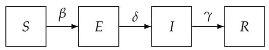
Figure 1. The Susceptible (S), Exposed (E), Infectious (I) and Removed (R) (SEIR) model.

1.1.2. Types of Epidemic Data

There are generally two types of epidemic data, temporal data and final size data [20]. Final size data do not show how the disease spreads over time during the epidemic; they only show snapshot information at the beginning and end of the outbreak. Temporal data, on the other hand, reveal details about the state of individuals during the epidemic. Data that contain both infection and removal times are referred to as complete temporal data, whereas data that only include removal times are referred to as partial temporal data. Temporal data may correspond to the times at which individuals are infected or removed.

1.1.3. The Basic Reproduction Number $R_0$

Threshold behavior is frequently shown in epidemic models. This roughly suggests that during an epidemic, either relatively few individuals become infected or a substantial number are infected. The basic reproduction number, $R_0$, which is heuristically defined as the average number of new infections brought on by a single infective in a large susceptible population, is a quantity of critical relevance in mathematical epidemic theory (see, e.g., [21]). This quantity is important because roughly speaking, in a population of infinitely many susceptibles, if $R_0\le 1$ then, with probability one, only a finite number of susceptibles will become infected (i.e., minor outbreak). However, if $R_0>1$ there is a positive probability that infinitely many susceptibles will become infected (i.e., major outbreak) and the disease becomes endemic. Knowledge of the value of $R_0$ makes it possible to calculate the proportion of a population that should be vaccinated in order to prevent an epidemic from spreading.

1.2. Marginal Likelihood Estimation

The marginal likelihood [22,23], also referred to as the evidence or integrated likelihood, is a quantity that gives a standard measure of the fit of a model in a Bayesian setting. Given multiple models that give reasonable predictions, the marginal likelihood of each model offers a mechanism to discriminate between them. What it gives is a measure of the likelihood of the data under the considered model. The issue is that, because it is often analytically challenging, computing the marginal likelihood is rarely straightforward, even in simple models. To calculate the marginal data densities in more complex models, high-dimensional integration is necessary. However, in majority of models, it is not possible to analytically integrate out parameters from the joint distribution for the data and the parameters. This means that numerical methods are required to obtain estimations, and these methods may be computationally costly.

The marginal likelihood could be formally defined as follows. Given a data set $\mathit{y}$, a statistical model M with parameter $\mathit{\theta }$, a prior distribution $\pi \left(\mathit{\theta }\right|M)$, a likelihood $\pi \left(\mathit{y}\right|\mathit{\theta },M)$ and a posterior distribution $\pi \left(\mathit{\theta }\right|\mathit{y},M)$, then $\pi \left(\mathit{y}\right|M)$ is the marginal likelihood of the model. It represents the likelihood of the data given the model. It can be calculated by using the equality

$$\pi \left(\mathit{y}\right|M)=\int \pi (\mathit{y}|\mathit{\theta },M)\pi \left(\mathit{\theta }\right|M)d\mathit{\theta },$$

where approximations shall be denoted as $\widehat{\pi \left(\mathit{y}\right)}$, and the conditioning on M shall be omitted for notational simplicity.

1.3. Bayes Factors

Bayes factor [23] is one of the most crucial tools for Bayesian model comparison and hypothesis testing. The Bayes factor, which enables model comparison, may be calculated once the marginal likelihood has been determined. Now, suppose there are two competing epidemic models, $M_i$ and $M_j$, with parameters ${\mathit{\theta }}_i$ and ${\mathit{\theta }}_j$, respectively, and $\mathit{y}$ is the observed data set. The Bayes factor in favor of model $M_i$ over model $M_j$ is then given by

$$B{F}_{ij}=\frac{\pi \left(\mathit{y}\right|M_i)}{\pi \left(\mathit{y}\right|M_j)}=\frac{\int \pi \left(\mathit{y}\right|{\mathit{\theta }}_i)\pi \left({\mathit{\theta }}_i\right)d{\mathit{\theta }}_i}{\int \pi \left(\mathit{y}\right|{\mathit{\theta }}_j)\pi \left({\mathit{\theta }}_j\right)d{\mathit{\theta }}_j},$$

where here, and throughout the paper, $\pi$ denotes a density function.

Analytical calculation of Bayes factors is often challenging. Moreover, the estimation of Bayes factors is, in general, difficult. Many approaches exist to estimate it, but here we focus specifically on simulation-based and easy-to-implement methods. The fact that these techniques are relatively prescriptive and provide the user with few implementation options that might substantially impact the performance of the resultant algorithms is one of its appealing features.

1.4. Model Selection within the Stochastic Epidemic Models Literature

There is currently no favored approach for model selection in the literature of epidemic modeling [11]. In the Bayesian setting, approaches include the use of Bayes factors [24,25,26,27], criteria such as the Deviance Information Criterion (DIC) [26,27,28], and methods based on the predictive distribution of future outbreaks [10,29]. Bayesian model selection tools have been applied to epidemic models with final size data and temporal data in certain scenarios. Here, we focus on the use of Bayes factors via marginal likelihood estimation.

The use of reversible jump Markov chain Monte Carlo techniques has been a common approach for computing Bayes factors for epidemics [24,25], although these methods are often problematic in practice due to the challenge of designing efficient algorithms. Given removal data, a combination of MCMC methods and importance sampling was used to estimate marginal likelihoods from which Bayes factors can be calculated [30]. A path-sampling method [31] was implemented to compare epidemic models given data on the final outcome of the epidemic in [26]. The power posterior approach [32] was extended and implemented for estimating the Bayes factor in the epidemic context where the epidemic data are only partially observed [27]. A more complete picture about this topic can be found in [10,11].

2. Bayesian Inference via MCMC Methods for the SEIR Model with Time-Dependent Infection Rate

2.1. Complete Data Case

Suppose that an SEIR system is considered and let m denote the number of individuals becoming infectious at times $\mathit{i}=(i_1,\dots ,i_m)$ and removed from the population at times $\mathit{r}=(r_1,\dots ,r_m)$ with $0=r_1\le r_2\le \dots \le r_m$. Similarly, let $\mathit{e}=\{e_j:j\ne \omega \}$ denote the set of the $m-1$ exposure times, that are the times at which individuals catch the infection but are unable to spread it, such that for $1\le j\le m,e_j$ refers to the exposure time of the individual who becomes infectious at time $i_j=e_j+l$ and recovered at time $r_j$, where the initial exposed individual is labeled by $\omega$ such that $e_{\omega }<e_j$ for all $j\ne \omega$.

Now, taking into account model $M_2$, the likelihood of the data given the model parameters may be written as

$$\begin{array}{ccc}\hfill L(\mathit{e},\mathit{i},\mathit{r}|\beta ,\psi ,\mathit{\theta },e_{\omega })& =& \left(\prod _{j=1,j\ne \omega }^m{h}_{\psi }(\beta ,e_j-)I(e_j-)\right)\times exp\left(-{\int }_{e_{\omega }}^{r_m}{h}_{\psi }(\beta ,t)S\left(t\right)I\left(t\right)dt\right)\hfill \\ & \times & \prod _{j=1}^m{f}_{D_I}\left(r_j-i_j|\mathit{\theta }\right),\hfill \end{array}$$

(1)

where $h_{\psi }(\beta ,s)=n^{-1}\beta e^{-\psi s}$, with $e_k=i_k=r_k=\infty$ for $k=m+1,\dots ,N$, and $\mathit{\theta }$ indicates the parameter governing the infectious period, $D_I$, where $\mathit{\theta }$ may be a vector.

Note that, when the infectious period distribution is exponential with rate $\gamma$ ( $r_j-i_j\sim Exp\left(\gamma \right)$), then

$$\begin{array}{c}\hfill \prod _{j=1}^m{f}_{D_I}\left(r_j-i_j|\mathit{\theta }\right)=\prod _{j=1}^m\gamma exp\left(-\gamma (r_j-i_j)\right)\end{array}$$

(2)

Given complete epidemic data, the Bayesian framework can first be used by assigning the model parameters’ independent conjugate gamma prior distributions as in [33], namely $\beta \sim \mathsf{\Gamma }({\lambda }_{\beta },{\nu }_{\beta })$, and $\gamma \sim \mathsf{\Gamma }({\lambda }_{\gamma },{\nu }_{\gamma })$. Then, the joint posterior density for $\beta$ and $\gamma$ (assuming $\psi$ is known) is obtained by multiplying the prior distributions and the likelihood as follows.

$$\begin{array}{ccc}\hfill \pi (\beta ,\gamma |\mathit{e},\mathit{i},\mathit{r},e_{\omega })& \propto & L(\mathit{e},\mathit{i},\mathit{r},e_{\omega }|\beta ,\gamma )\pi \left(\beta \right)\pi \left(\gamma \right)\hfill \\ & =& \left(\prod _{j=1,j\ne \omega }^m{n}^{-1}\beta e^{-\psi e_j-}I(e_j-)\right)\times exp\left(-n^{-1}\beta {\xi }_{\psi }\right)\hfill \\ & \times & \prod _{j=1}^m\gamma exp\left(-\gamma (r_j-i_j)\right)\times {\beta }^{{\lambda }_{\beta }-1}{e}^{-{\nu }_{\beta }\beta }\times {\gamma }^{{\lambda }_{\gamma }-1}{e}^{-{\nu }_{\gamma }\gamma },\hfill \end{array}$$

(3)

where

$${\xi }_{\psi }={\int }_{e_{\omega }}^{r_m}{e}^{-\psi t}S\left(t\right)I\left(t\right)dt.$$

The parameters $\beta$ and $\gamma$ are a posteriori conditionally independent, so we have

$$\pi \left(\beta \right|\mathit{e},e_{\omega },\mathit{i},\mathit{r})\equiv \mathsf{\Gamma }\left({\lambda }_{\beta }+m-1,{\nu }_{\beta }+n^{-1}{\xi }_{\psi }\right),$$

(4)

$$\pi \left(\gamma \right|\mathit{e},e_{\omega },\mathit{i},\mathit{r})\equiv \mathsf{\Gamma }\left({\lambda }_{\gamma }+m,{\nu }_{\gamma }+\sum _{j=1}^m(r_j-i_j)\right).$$

(5)

The posterior distributions of the two parameters, $\beta$ and $\gamma$, are thus easily accessible, making it simple to obtain any function of these parameters.

Note that the inference for models $M_1$ and $M_3$, given complete data, can be performed in a similar manner (see, e.g., [10,14]).

2.2. Incomplete Data Case

When the exposure times and hence the infection times are not observed, the likelihood of the removal times becomes intractable. A common way to handle this issue is to use data augmentation technique [34,35] by treating the missing data as extra parameters to be inferred from the data [33].

We again derive the following full conditional posterior distributions by assigning independent conjugate gamma prior distributions for the model parameters $\beta$ and $\gamma$, and further assuming $e_{\omega }$ has an improper uniform prior density on $(-\infty ,r_1)$,

$$\pi \left(\beta \right|\gamma ,\mathit{e},e_{\omega },\mathit{i},\mathit{r})\equiv \mathsf{\Gamma }\left({\lambda }_{\beta }+m-1,{\nu }_{\beta }+n^{-1}{\xi }_{\psi }\right),$$

(6)

$$\pi \left(\gamma \right|\beta ,\mathit{e},e_{\omega },\mathit{i},\mathit{r})\equiv \mathsf{\Gamma }\left({\lambda }_{\gamma }+m,{\nu }_{\gamma }+\sum _{j=1}^m(r_j-i_j)\right),$$

(7)

and

$$\pi (\mathit{i},\mathit{e},e_{\omega }|\beta ,\gamma ,\mathit{r})\propto \prod _{j=1,j\ne \omega }^m{e}^{-\psi e_j-}I(e_j-)\times exp\left(-\beta n^{-1}{\xi }_{\psi }\right)\times \prod _{j=1}^{m}exp\left(-\gamma (r_j-i_j)\right).$$

(8)

Given that the model parameters $\beta$ and $\gamma$ have closed forms of the posterior distribution, updating them can be performed via Gibbs sampling steps [10,33,36]. However, as the posterior distribution of the component $(\mathit{i},\mathit{e},e_{\omega })$ is not explicitly provided, it needs to be updated using the Metropolis–Hastings step. In general, it is possible to apply (with minor adjustments) the MCMC technique in [10,33] to update both the model parameters and the missing exposure and infection times. Bayesian inference for models $M_1$ and $M_3$ can be performed in a similar way (see, e.g., [10,27]).

However, the focus of this paper is on model choice given complete epidemic data, where we aim to derive explicit expressions for the Bayes factor in asymmetric infection process settings to validate the estimate of the Bayes factor derived from other proposed methods.

2.3. The Behavior of the SEIR Models Featuring Asymmetrical Dynamics of Transmission

One crucial issue of special significance when modeling an infectious disease is how infectious the disease is. The rate at which individuals contract a disease, in other words. The use of strategies to stop the spread of a disease among a population can be facilitated by having access to such knowledge. The effective of having different infection processes can be observed by comparing the removal trajectories and the epidemic duration for an epidemic.

The behavior of models $M_1$ and $M_3$ was investigated using the removal trajectories and the outbreak duration. A simulation study was conducted to investigate how the two SEIR models behave. We simulated 5000 removal trajectories from each SEIR model with $\beta =0.5,\gamma =0.2$ for the $M_1$ model and $\beta =3,\gamma =0.2,\psi =0.3$ for the $M_3$ model, using a population of size $N=100(n=99,k=1)$.

The major outbreak components of the final size distributions were permitted to be comparable in the sense that they peaked at around the same values for both models, and we set the mean infectious period to be the same in both models ($1/\gamma =5$). The length of the latent period was set at $l=1$ in both models.

It is clear from Figure 2 that the removal trajectory distributions of the two SEIR models differ in terms of their position and shape. In particular, the $M_1$ model peaks quicker and has more variants, whereas the $M_3$ model tends to be more widespread and has a longer epidemic duration.

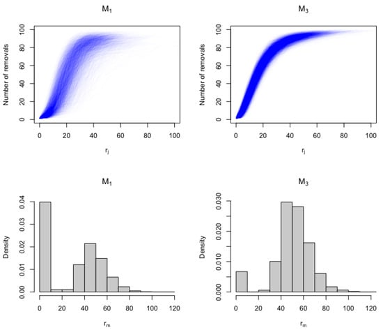
Figure 2. The distributions of removal trajectories and epidemic duration are represented by the top and bottom rows, respectively. The distributions of 5000 removal curves that were simulated from each SEIR model are displayed in the first row. The distributions of the epidemic duration ($r_m$) from each SEIR model based on the 5000 simulated epidemics are displayed in the second row.

3. Bayes Factors and Marginal Likelihood Estimation for SEIR Epidemic Models Given Complete Data

In this section, assuming complete outbreak data, we shall derive explicit expressions for the Bayes factor across several epidemic scenarios. This assumption could be unrealistic in practice, although it may arise when outbreaks are being closely monitored. For instance, complete data can be gathered in the early phases of a suspected major epidemic, or in experimental settings for animal diseases. The motivations for looking at Bayes factor formula are that it is of interest in its own right and it provides us of some insights into how to better comprehend this Bayesian model selection tool. In addition, we can validate the estimate of the Bayes factor derived from other methods proposed in the literature such as the arithmetic mean and harmonic mean methods in order to see how reliable they are in situations where complete epidemic data are available but Bayes factors cannot be obtained in closed forms.

3.1. Bayes Factors: Theoretical Aspects

The Bayes factor in favor of model $M_1$ over model $M_2$ can be calculated as follows.

$$\begin{array}{ccc}\hfill B{F}_{12}& =& \frac{\pi (\mathit{e},e_{\omega },\mathit{i},\mathit{r}|M_1)}{\pi (\mathit{e},e_{\omega },\mathit{i},\mathit{r}|M_2)}\hfill \\ & =& \frac{{\int }_{\gamma }{\int }_{\beta }\pi (\mathit{e},e_{\omega },\mathit{i},\mathit{r}|\beta ,\gamma )\pi \left(\beta \right)\pi \left(\gamma \right)d\beta d\gamma }{{\int }_{\gamma }{\int }_{\beta }\pi (\mathit{e},e_{\omega },\mathit{i},\mathit{r}|\beta ,\gamma ,\psi )\pi \left(\beta \right)\pi \left(\gamma \right)d\beta d\gamma }\hfill \end{array}$$

(9)

The epidemic likelihood may be broken into two independent (infection and removal) parts and, as the removal processes are the same for both SEIR models, they are canceled out. Therefore, we have the following Bayes factor expression:

$$\begin{array}{ccc}\hfill B{F}_{12}& =& \frac{{\nu }_{\beta }^{{\lambda }_{\beta }}\mathsf{\Gamma }\left({\lambda }_{\beta }\right)}{{\nu }_{\beta }^{{\lambda }_{\beta }}\mathsf{\Gamma }\left({\lambda }_{\beta }\right)}\times \frac{{\prod }_{j=1,j\ne \omega }^m{n}^{-1}I(e_j-)}{{\prod }_{j=1,j\ne \omega }^m{n}^{-1}{e}^{-\psi e_j-}I(e_j-)}\times \frac{{\int }_{\beta }{\beta }^{m-1}\times e^{-\beta n^{-1}\xi }\times {\beta }^{{\lambda }_{\beta }-1}{e}^{-{\nu }_{\beta }\beta }d\beta }{{\int }_{\beta }{\beta }^{m-1}\times e^{-\beta n^{-1}{\xi }_{\psi }}\times {\beta }^{{\lambda }_{\beta }-1}{e}^{-{\nu }_{\beta }\beta }d\beta }\hfill \\ & =& exp\left(\psi \sum _{j=1,j\ne \omega }^m{e}_j-\right)\times {\left(\frac{{\nu }_{\beta }+n^{-1}{\xi }_{\psi }}{{\nu }_{\beta }+n^{-1}\xi }\right)}^{m-1+{\lambda }_{\beta }},\hfill \end{array}$$

(10)

where

$$\xi ={\int }_{e_{\omega }}^{r_m}S\left(t\right)I\left(t\right)dt;{\xi }_{\psi }={\int }_{e_{\omega }}^{r_m}{e}^{-\psi t}S\left(t\right)I\left(t\right)dt.$$

Now, we have ${\xi }_{\psi }<\xi$ as $0<e^{-\psi t}<1$, therefore $B{F}_{12}$ has an upper bound, that is

$$B{F}_{12}<exp\left(\psi \sum _{j=1,j\ne \omega }^m{e}_j-\right).$$

In addition, to see the impact of the infection rate prior distribution on the behavior of $B{F}_{12}$, we rewrite $B{F}_{12}$ in terms of the mean and variance of the prior distribution, that are

$$E\left[\mathsf{\Gamma }({\lambda }_{\beta },{\nu }_{\beta })\right]={\lambda }_{\beta }/{\nu }_{\beta }=\mu \mathrm{and}\mathrm{Var}\left[\mathsf{\Gamma }({\lambda }_{\beta },{\nu }_{\beta })\right]={\lambda }_{\beta }/{\nu }_{\beta }^2={\sigma }^2,$$

which implies ${\lambda }_{\beta }={\mu }^2/{\sigma }^2$ and ${\nu }_{\beta }=\mu /{\sigma }^2$. Substituting these values into (10) yields

$$B{F}_{12}=exp\left(\psi \sum _{j=1,j\ne \omega }^m{e}_j-\right)\times {\left(\frac{\frac{\mu }{{\sigma }^2}+\frac{{\xi }_{\psi }}{n}}{\frac{\mu }{{\sigma }^2}+\frac{\xi }{n}}\right)}^{m-1+\frac{{\mu }^2}{{\sigma }^2}}.$$

(11)

Consequently, as ${\sigma }^2\to \infty$ or ${\sigma }^2\to 0$, we have the following limits for the Bayes factor $B{F}_{12}$, namely

$$B{F}_{12}\to {({\xi }_{\psi }/\xi )}^{m-1}\times exp\left(\psi \sum _{j=1,j\ne \omega }^m{e}_j-\right),\mathrm{as}{\sigma }^2\to \infty ,$$

(12)

and

$$B{F}_{12}\to exp\left(\psi \sum _{j=1,j\ne \omega }^m{e}_j-\right),\mathrm{as}{\sigma }^2\to 0.$$

(13)

It can be noticed that as the prior becomes more and more concentrated at $\mu$ (${\sigma }^2\to 0$), the Bayes factor becomes more decisive in supporting $M_1$.

Similarly, the Bayes factor in favor of model $M_2$ over model $M_3$ can be obtained as follows.

$$\begin{array}{ccc}\hfill B{F}_{23}& =& \frac{\pi (\mathit{e},e_{\omega },\mathit{i},\mathit{r}|M_2)}{\pi (\mathit{e},e_{\omega },\mathit{i},\mathit{r}|M_3)}\hfill \\ & =& \frac{{\nu }_{\beta }^{{\lambda }_{\beta }}\mathsf{\Gamma }\left({\lambda }_{\beta }\right)}{{\nu }_{\beta }^{{\lambda }_{\beta }}\mathsf{\Gamma }\left({\lambda }_{\beta }\right)}\times \frac{{\prod }_{j=1,j\ne \omega }^m{n}^{-1}{e}^{-\psi e_j-}I(e_j-)}{{\prod }_{j=1,j\ne \omega }^m{n}^{-1}{I}^{\zeta }(e_j-)}\times \frac{{\int }_{\beta }{\beta }^{m-1}\times e^{-\beta n^{-1}{\xi }_{\psi }}\times {\beta }^{{\lambda }_{\beta }-1}{e}^{-{\nu }_{\beta }\beta }d\beta }{{\int }_{\beta }{\beta }^{m-1}\times e^{-\beta n^{-1}{\xi }_{\zeta }}\times {\beta }^{{\lambda }_{\beta }-1}{e}^{-{\nu }_{\beta }\beta }d\beta }\hfill \\ & =& exp\left(-\psi \sum _{j=1,j\ne \omega }^m{e}_j-\right)\times \left(\prod _{j=1,j\ne \omega }^m{I}^{1-\zeta }(e_j-)\right)\times {\left(\frac{{\nu }_{\beta }+n^{-1}{\xi }_{\zeta }}{{\nu }_{\beta }+n^{-1}{\xi }_{\psi }}\right)}^{m-1+{\lambda }_{\beta }},\hfill \end{array}$$

(14)

where,

$${\xi }_{\zeta }={\int }_{e_{\omega }}^{r_m}S\left(t\right)I^{\zeta }\left(t\right)dt.$$

By rewriting $B{F}_{23}$ in terms of the mean and variance of the prior distribution, we have

$$B{F}_{23}=exp\left(-\psi \sum _{j=1,j\ne \omega }^m{e}_j-\right)\times \left(\prod _{j=1,j\ne \omega }^m{I}^{1-\zeta }(e_j-)\right)\times {\left(\frac{\frac{\mu }{{\sigma }^2}+\frac{{\xi }_{\zeta }}{n}}{\frac{\mu }{{\sigma }^2}+\frac{{\xi }_{\psi }}{n}}\right)}^{m-1+\frac{{\mu }^2}{{\sigma }^2}}.$$

(15)

Consequently, as ${\sigma }^2\to \infty$ or ${\sigma }^2\to 0$, we have the following limits for the Bayes factor $B{F}_{23}$, namely

$$B{F}_{23}\to {({\xi }_{\zeta }/{\xi }_{\psi })}^{m-1}\times exp\left(-\psi \sum _{j=1,j\ne \omega }^m{e}_j-\right)\times \left(\prod _{j=1,j\ne \omega }^m{I}^{1-\zeta }(e_j-)\right),\mathrm{as}{\sigma }^2\to \infty ,$$

(16)

and

$$B{F}_{23}\to exp\left(-\psi \sum _{j=1,j\ne \omega }^m{e}_j-\right)\times \left(\prod _{j=1,j\ne \omega }^m{I}^{1-\zeta }(e_j-)\right),\mathrm{as}{\sigma }^2\to 0.$$

(17)

It is evident that decreasing the prior uncertainty leads to favoring the $M_2$ model.

These theoretical aspects and explicit Bayes factor expressions are of particular assistance in gaining some insights into what estimated values of Bayes factors might be expected, specifically under different prior assumptions. For this particular epidemic setting, we may conclude that increasing (decreasing) the prior uncertainty of the model parameters reduces (increases) the Bayes factor value.

As an aside, one should be aware of any potential connections to Lindley’s paradox [37] when employing the Bayes factor criteria to conduct a Bayesian model choice task. However, in this epidemic setting, models are not nested and have the same level of complexity.

Prior Sensitivity Simulation Study

It is well known that Bayes factors can exhibit strong dependence on the within-model prior distributions [38]. In our epidemic setting, we explore this issue in detail, considering what happens to the Bayes factors for an asymmetrical diffuse prior distribution. A typical case in practice is when ${\lambda }_{\beta }=1$ and ${\nu }_{\beta }\to 0$ (see, e.g., [27,39,40]).

Figure 3 (left) shows $log\left(B{F}_{12}\right)$ values for some complete epidemic data generated under model $M_1$ in a closed population of size $N=100(n=99,k=1)$, 92 of whom were infected, with parameter values $\beta =3,\gamma =1,l=1$. The parameter $\psi$ in model $M_2$ was set to $0.1$, and then $log\left(B{F}_{12}\right)$ was calculated for various values of ${\nu }_{\beta }$. It is clear that as the prior become more informative (i.e., ${\nu }_{\beta }$ increases), the $log\left(B{F}_{12}\right)$ becomes more supportive to the data-generating model $M_1$.

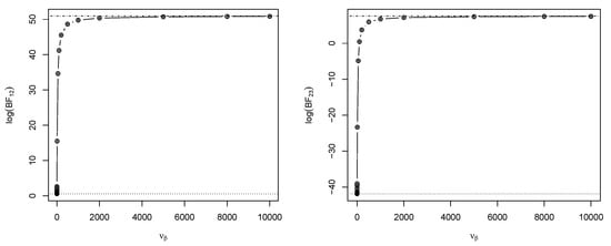
Figure 3. Values of $log\left(B{F}_{12}\right)$ (left) and $log\left(B{F}_{23}\right)$ (right), calculated for various ${\nu }_{\beta }$ (the $\beta$ prior scale parameter) with ${\lambda }_{\beta }=1$ fixed. The horizontal dashed lines denote the lower and upper limiting values of $log\left(B{F}_{12}\right)$ and $log\left(B{F}_{23}\right)$ as ${\nu }_{\beta }$ varies.

Figure 3 (right) shows $log\left(B{F}_{23}\right)$ values for some complete epidemic data generated under model $M_3$ in a closed population of size $N=100(n=99,k=1)$, 92 of whom were infected, with parameter values $\beta =7.5,\gamma =1,l=1,\zeta =0.3$. Again, we set $\psi =0.1$ in model $M_2$, and then $log\left(B{F}_{23}\right)$ was calculated for various values of ${\nu }_{\beta }$. It is evident that as ${\nu }_{\beta }$ increases (the prior becomes more informative), the $log\left(B{F}_{23}\right)$ tends to favor the true model $M_3$.

3.2. Computational Methods for Marginal Likelihood Estimation

As introduced earlier, $(\mathit{e},e_{\omega }),\mathit{i}$ and $\mathit{r}$ denote the observed exposure, infection and removal times, respectively, with $\beta$ and $\gamma$ representing the models’ infection and removal rates parameters. Here we discuss three computational methods to estimate the marginal likelihood presented in the literature of model choice but not applied in model selection of stochastic epidemic models. The rationale is to see how robust and reliable they are when considering dependent data with complex likelihoods such as the ones involved in our epidemic models settings.

3.2.1. Arithmetic Mean Estimator (Naive Monte Carlo Estimator)

Dropping the notational dependence on M, the marginal likelihood becomes

$$\pi (\mathbf{e},e_{\omega },\mathit{i},\mathit{r})={\int }_{\gamma }{\int }_{\beta }\pi (\mathit{e},e_{\omega },\mathit{i},\mathit{r}|\beta ,\gamma )\pi (\beta ,\gamma )d\beta d\gamma .$$

(18)

The arithmetic mean (AM) estimator for $\pi (\mathit{e},e_{\omega },\mathit{i},\mathit{r})$ can be obtained by a simple Monte Carlo integration method, that is

$$\widehat{\pi (\mathit{e},e_{\omega },\mathit{i},\mathit{r})}=\frac{1}{K}\sum _{h=1}^K\pi (\mathit{e},e_{\omega },\mathit{i},\mathit{r}|{\beta }^{\left(h\right)},{\gamma }^{\left(h\right)}),$$

(19)

where ${\beta }^{\left(1\right)},\dots ,{\beta }^{\left(K\right)}$ and ${\gamma }^{\left(1\right)},\dots ,{\gamma }^{\left(K\right)}$ are samples generated from the priors $\pi \left(\beta \right)$ and $\pi \left(\gamma \right)$, respectively.

It is well-known [23] that since the likelihood is typically sharply peaked, most of the prior samples have very small likelihood values, in particular when the prior is diffuse. Therefore, unless K is very large, the prior samples will contain virtually no points from the high-likelihood region, leading to poor and inadequate estimation of the marginal likelihood. However, by the law of large numbers, this estimator converges to the true expectation as the number of independent samples, K, drawn from the prior, tends to infinity [41]. Additionally, this estimate can perform well when the dimensionality of the parameter space is modest, so that enormous prior samples can be generated very quickly.

• Illustrative simulation study

In what follows, we conducted a simulation study to illustrate the effectiveness of the AM estimator of the marginal likelihood in approximating the true marginal likelihood and hence the Bayes factor. This simulation example was performed under different prior assumptions for each model parameter. As we have a prior of two dimensions in each model, $M_1,M_2$ and $M_3$, we expect the arithmetic mean estimates of the marginal likelihoods, namely

$$\widehat{\pi (\mathit{e},e_{\omega },\mathit{i},\mathit{r}|M_1)}=\frac{1}{K}\sum _{h=1}^K\pi (\mathit{e},e_{\omega },\mathit{i},\mathit{r}|{\beta }^{\left(h\right)},{\gamma }^{\left(h\right)}),$$

(20)

$$\widehat{\pi (\mathit{e},e_{\omega },\mathit{i},\mathit{r}|M_2)}=\frac{1}{K}\sum _{h=1}^K\pi (\mathit{e},e_{\omega },\mathit{i},\mathit{r}|\psi ,{\beta }^{\left(h\right)},{\gamma }^{\left(h\right)}),$$

(21)

and

$$\widehat{\pi (\mathit{e},e_{\omega },\mathit{i},\mathit{r}|M_3)}=\frac{1}{K}\sum _{h=1}^K\pi (\mathit{e},e_{\omega },\mathit{i},\mathit{r}|\zeta ,{\beta }^{\left(h\right)},{\gamma }^{\left(h\right)}),$$

(22)

to be effective in the estimating and recovering the true value of the Bayes factor. Here, ${\beta }^{\left(h\right)}$ and ${\gamma }^{\left(h\right)}$, where $h=1,2,\dots ,K$, are independent samples drawn from the gamma prior distribution.

We simulated two typical epidemic data sets, one data set was generated under $M_1$ and the other data set was simulated from $M_3$. Each outbreak was in a closed population consisting of 99 initially susceptible individuals and a single initially infected case. The model parameters for the simulation were ($\beta =3,\gamma =1,l=1$) for model $M_1$ and ($\beta =7,\gamma =1,l=1,\zeta =0.3$) for model $M_3$. The resulting final size was 92 under both models. The parameter $\psi$ was set to $0.1$ when fitting $M_2$.

Under each prior assumption, namely $\mathsf{\Gamma }(1,1),\mathsf{\Gamma }(1,0.1)$ and $\mathsf{\Gamma }(1,0.01)$, the true values of the logarithm of Bayes factors were calculated using (10) and (14). The estimated values of the logarithm of Bayes factors, under different prior distributions, were computed as follows. Initially, we simulated K samples from the prior for each parameter and evaluated the marginal likelihoods based on these prior samples using (20)–(22). Then, the logarithm of Bayes factors was estimated using the following equations.

$$log\left(\widehat{B{F}_{12}}\right)=log\left[\widehat{\pi (\mathit{e},e_{\omega },\mathit{i},\mathit{r}|M_1)}\right]-log\left[\widehat{\pi (\mathit{e},e_{\omega },\mathit{i},\mathit{r}|M_2)}\right],$$

(23)

$$log\left(\widehat{B{F}_{23}}\right)=log\left[\widehat{\pi (\mathit{e},e_{\omega },\mathit{i},\mathit{r}|M_2)}\right]-log\left[\widehat{\pi (\mathit{e},e_{\omega },\mathit{i},\mathit{r}|M_3)}\right].$$

(24)

The results are displayed in Table 1. It was found that increasing prior uncertainty of the model parameters does not have much effect on the precision of Bayes factor estimation via AM method, as the prior in our case is low-dimensional and so fast to sample from. These results suggest that as the flat prior distribution expresses a form of neutrality and lack of previous knowledge, its use is possible in the present application. In contrast, a more informative prior (e.g., $\mathsf{\Gamma }(1,1)$) also has the advantage of estimating $log\left(B{F}_{12}\right)$ and $log\left(B{F}_{23}\right)$ more accurately. These results indicate the possibility of using the arithmetic mean estimator of the marginal likelihood as a simple but effective way of approximating Bayes factors in situations where complete epidemic data are available but Bayes factors cannot be obtained in a closed form. For instance, when comparing these SEIR models with unknown $\psi$ or when comparing the SEIR model with different infection mechanisms and unknown power parameter $\zeta$.

Table 1. The logarithm of Bayes factor results obtained using two data sets simulated based on models $M_1$ and $M_3$. For each case, model parameters were assigned prior distributions to varying degrees of diffuseness to determine the effect on the logarithm of Bayes factor estimation. Three sizes of prior parameter sample ($K={10}^4,K={10}^5$ and $K={10}^6$) were used to determine the effective sample size required to reasonably estimate the logarithm of Bayes factor.

Model	Prior	True$\log \left({\mathit{BF}}_{12}\right)$	$\log \left(\widehat{{\mathit{BF}}_{12}}\right)$
			$\mathbf{K}\mathbf{=}{\mathbf{10}}^{\mathbf{4}}$	$\mathbf{K}\mathbf{=}{\mathbf{10}}^{\mathbf{5}}$	$\mathbf{K}\mathbf{=}{\mathbf{10}}^{\mathbf{6}}$
	$\mathsf{\Gamma }(1,1)$	$3.894706$	$3.995201$	$3.835836$	$3.899106$
$M_1$	$\mathsf{\Gamma }(1,0.1)$	$1.811504$	$2.035148$	$1.817458$	$1.815973$
	$\mathsf{\Gamma }(1,0.01)$	$1.593932$	$0.9698732$	$1.859154$	$1.6351788$
		True $\mathbf{log}\mathbf{\left(}{\mathit{BF}}_{\mathbf{23}}\mathbf{\right)}$	$\mathbf{log}\mathbf{\left(}\widehat{{\mathit{BF}}_{\mathbf{23}}}\mathbf{\right)}$
			$\mathbf{K}\mathbf{=}{\mathbf{10}}^{\mathbf{4}}$	$\mathbf{K}\mathbf{=}{\mathbf{10}}^{\mathbf{5}}$	$\mathbf{K}\mathbf{=}{\mathbf{10}}^{\mathbf{6}}$
	$\mathsf{\Gamma }(1,1)$	$-28.08603$	$-28.59146$	$-28.3244$	$-28.04024$
$M_3$	$\mathsf{\Gamma }(1,0.1)$	$-30.5115$	$-31.30335$	$-30.35625$	$-30.49217$
	$\mathsf{\Gamma }(1,0.01)$	$-30.767$	$-35.95646$	$-31.66247$	$-30.71537$

3.2.2. Harmonic Mean Method

Estimation of the marginal likelihood by harmonic mean approach has become a popular method due to its simplicity. The harmonic mean (HM) estimator was first proposed by [42] who showed that the marginal likelihood can be estimated from the harmonic mean of the likelihood, given posterior samples. Under the assumption that the prior distribution of the parameters is proper, we have

$$1={\int }_{\gamma }{\int }_{\beta }\pi (\beta ,\gamma )d\beta d\gamma =\pi (\mathit{e},e_{\omega },\mathit{i},\mathit{r}){\int }_{\gamma }{\int }_{\beta }\frac{1}{\pi (\mathit{e},e_{\omega },\mathit{i},\mathit{r}|\beta ,\gamma )}\pi (\beta ,\gamma |\mathit{e},e_{\omega },\mathit{i},\mathit{r})d\beta d\gamma .$$

Therefore,

$$\frac{1}{\pi (\mathit{e},e_{\omega },\mathit{i},\mathit{r})}={\int }_{\gamma }{\int }_{\beta }\frac{1}{\pi (\mathit{e},e_{\omega },\mathit{i},\mathit{r}|\beta ,\gamma )}\pi (\beta ,\gamma |\mathit{e},e_{\omega },\mathit{i},\mathit{r})d\beta d\gamma =E_{(\beta ,\gamma |\mathit{e},e_{\omega },\mathit{i},\mathit{r})}\left(\frac{1}{\pi (\mathit{e},e_{\omega },\mathit{i},\mathit{r}|\beta ,\gamma )}\right),$$

where $E_{(\beta ,\gamma |\mathit{e},e_{\omega },\mathit{i},\mathit{r})}$ denotes the expected value with respect to the posterior distribution of the models parameters.

The harmonic mean estimator is given by

$$\widehat{\pi (\mathit{e},e_{\omega },\mathit{i},\mathit{r})}={\left(\frac{1}{K}\sum _{h=1}^K\frac{1}{\pi (\mathit{e},e_{\omega },\mathit{i},\mathit{r}|{\beta }^{\left(h\right)},{\gamma }^{\left(h\right)})}\right)}^{-1},$$

(25)

where $\{{\beta }^{\left(1\right)},\dots ,{\beta }^{\left(K\right)}\}$ and $\{{\gamma }^{\left(1\right)},\dots ,{\gamma }^{\left(K\right)}\}$ are sets of MCMC draws from the posterior distribution.

The simplicity (easy and fast) of the HM approach is its main advantage over other more specialized techniques. It uses only within-model posterior samples and likelihood evaluations, which are often available anyway as part of posterior sampling. This estimator is consistent, but sometimes its variance can be large, since occasionally a sample may be taken into consideration with low likelihood, which significantly affects the result due to the reciprocal presented in (25). The HM estimator is often biased and results in overestimating the true marginal likelihood [43]. It is included here because of its simplicity and being not applied as a model selection tool in stochastic epidemic modeling.

3.2.3. Power Posterior Method

An approach for estimating the marginal likelihood based on the idea of thermodynamic integration [31] was developed in [32]. The authors introduced an auxiliary variable (temperature parameter) $p\in [0,1]$ and defined the power posterior (PP) as

$${\pi }_p(\beta ,\gamma |\mathit{e},e_{\omega },\mathit{i},\mathit{r})\propto \pi {(\mathit{e},e_{\omega },\mathit{i},\mathit{r}|\beta ,\gamma )}^p\pi (\beta ,\gamma ),$$

(26)

where by construction the normalizing constant of the power posterior is

$$z_p(\mathit{e},e_{\omega },\mathit{i},\mathit{r})={\int }_{\gamma }{\int }_{\beta }\pi {(\mathit{e},e_{\omega },\mathit{i},\mathit{r}|\beta ,\gamma )}^p\pi (\beta ,\gamma )d\beta d\gamma .$$

(27)

Clearly, as p moves from $p=0$ to $p=1$, the power posterior follows a path from the prior to the posterior density, where $z_{p=0}(\mathit{e},e_{\omega },\mathit{i},\mathit{r})=1$ is the integral of the proper prior of $(\beta ,\gamma )$ and $z_{p=1}(\mathit{e},e_{\omega },\mathit{i},\mathit{r})$ is the marginal likelihood. It can be shown that

$$log\left[\pi (\mathit{e},e_{\omega },\mathit{i},\mathit{r})\right]=log\left[\frac{z_{p=1}(\mathit{e},e_{\omega },\mathit{i},\mathit{r})}{z_{p=0}(\mathit{e},e_{\omega },\mathit{i},\mathit{r})}\right]={\int }_0^1{E}_{\beta ,\gamma |\mathit{e},e_{\omega },\mathit{i},\mathit{r},p}log\left[\pi (\mathit{e},e_{\omega },\mathit{i},\mathit{r}|\beta ,\gamma )\right]dp.$$

(28)

In [44], the approach was refined so that the power posterior estimate of $log\left[\pi (\mathit{e},e_{\omega },\mathit{i},\mathit{r}]\right)$ becomes

$$log\left[\pi (\mathit{e},e_{\omega },\mathit{i},\mathit{r})\right]\approx \sum _{j=1}^r\frac{1}{2}(p_j-p_{j-1})\times [{\Delta }_{p_j}+{\Delta }_{p_{j-1}}]-\sum _{j=1}^r\frac{1}{12}{(p_j-p_{j-1})}^2\times [{\mathsf{\Phi }}_{p_j}-{\mathsf{\Phi }}_{p_{j-1}}],$$

(29)

where

$${\Delta }_q=E_{\beta ,\gamma |\mathit{e},e_{\omega },\mathit{i},\mathit{r},q}log\left[\pi (\mathit{e},e_{\omega },\mathit{i},\mathit{r}|\beta ,\gamma )\right];q=p_j,p_{j-1},$$

and

$${\mathsf{\Phi }}_q=V_{\beta ,\gamma |\mathit{e},e_{\omega },\mathit{i},\mathit{r},q}log\left[\pi (\mathit{e},e_{\omega },\mathit{i},\mathit{r}|\beta ,\gamma )\right];q=p_j,p_{j-1},$$

are the expectation and the variance of $log\left[\pi (\mathit{e},e_{\omega },\mathit{i},\mathit{r}|\beta ,\gamma )\right]$ at q, respectively; and r is the number of points in the interval $(0,1]$ in the temperature schedule.

When considering $M_2$ model ($M_1$ and $M_3$ are performed similarly), at temperature p, the power posterior densities for $\beta$ and $\gamma$ can be obtained using (26), which gives

$${\pi }_p\left(\beta \right|\mathit{e},e_{\omega },\mathit{i},\mathit{r})\equiv \mathsf{\Gamma }\left({\lambda }_{\beta }+p(m-1),{\nu }_{\beta }+(p/n){\xi }_{\psi }\right),$$

(30)

$${\pi }_p\left(\gamma \right|\mathit{e},e_{\omega },\mathit{i},\mathit{r})\equiv \mathsf{\Gamma }\left({\lambda }_{\gamma }+m,{\nu }_{\gamma }+p\sum _{j=1}^m(r_j-i_j)\right).$$

(31)

More details about this method when applied to stochastic epidemic outbreak data can be found in [10,27], where the performance of this approach in estimating Bayes factors was investigated and assessed.

4. Extensive Simulation Study

In this section, we present an extensive simulation study for the three considered approaches in which the true values of the marginal likelihoods and hence Bayes factors are known (i.e., can be calculated analytically). Throughout this section, we assumed a fixed latent period of $l=1$, and we chose $\gamma =1$. Then, two simulated scenarios were preformed, each scenario was based on 120 epidemic outbreak data sets. These epidemic data sets were simulated using various population sizes ($N=10,50,100$) and fitted under two asymmetric prior assumptions, namely $\mathsf{\Gamma }(1,1)$ and $\mathsf{\Gamma }(1,0.01)$.

To make each of the approaches (AM, HM and PP) for computing the evidence as comparable as possible, we tried to make each of the algorithms equivalent in terms of the number of iterations. Therefore, the results were based on a run of 100,000 after a burn-in period of 5000 iterations, and thinning the chain by taking each 5th value. Table 2 summarized the two simulated scenarios.

Table 2. Details of the extensive simulation study in which each simulation scenario consists of 120 outbreak data sets generated under various population sizes and fitted under different prior assumptions.

Scenario	True Model	Fitted Models	Parameter Values
I	$M_1$	$M_1,M_2$	$\beta =2,2.5,3;\psi =0.1;r=20,40$
II	$M_3$	$M_2,M_3$	$\beta =3,5,7.5;\psi =0.1;\zeta =0.3;r=20,40$

4.1. Scenario I

In this simulated scenario, the data-generating model was $M_1$, where, using each population size, $N=10,50$ and 100, 20 outbreak data sets were generated. Then, under the two prior assumptions, namely $\mathsf{\Gamma }(1,1)$ and $\mathsf{\Gamma }(1,0.01)$, the true values of the $logB{F}_{12}$ were calculated using (10) and the $log\left(\widehat{B{F}_{12}}\right)$ values were computed using AM, HM and PP methods and their means over the 20 data sets are presented in Table 3, where each row gives results from 20 simulated epidemics in which the final sizes are matched to m.

Table 3. Results of the true mean values of $logB{F}_{12}$ and the estimated mean of $log\left(\widehat{B{F}_{12}}\right)$ computed using AM, HM and PP methods using different population sizes and two prior distribution settings. Each row gives results from 20 simulated epidemics in which the final sizes are matched to m.

Model	N	m	Prior	$\mathit{E}[log\left(\widehat{{\mathit{BF}}_{12}}\right)]$
				True	AM	HM	PP
$M_1$	10	8	$\mathsf{\Gamma }(1,1)$	0.1363	0.1373	0.1172	0.1367
			$\mathsf{\Gamma }(1,0.01)$	−0.4487	−0.4738	−0.3657	−0.4499
$M_1$	50	45	$\mathsf{\Gamma }(1,1)$	2.2709	2.2569	1.4543	2.2715
			$\mathsf{\Gamma }(1,0.01)$	0.8469	0.6860	1.5133	0.8486
$M_1$	100	90	$\mathsf{\Gamma }(1,1)$	1.8638	1.8609	0.5455	1.8627
			$\mathsf{\Gamma }(1,0.01)$	0.8393	0.8841	1.4024	0.8391

Surprisingly, in this experiment, the AM approach performed very well. This might be a result of having low-dimensional parameter space in our setting. The poorest performance was from the HM estimator. The PP method proved its robustness in estimating Bayes factors.

The mean values of the $logB{F}_{12}$ and the means of $log\left(\widehat{B{F}_{12}}\right)$ indicated that as the prior becomes diffuse, the true value of Bayes factors and their estimates using all approaches decrease. In addition to that, the values of Bayes factor were sensitive to epidemic data and were independent of the epidemic sizes. Another point to be mentioned here is that, with small outbreaks, having a vague prior distribution is not recommended and can affect this diagnostic tool for model choice as seen in Table 3 (the fourth row).

4.2. Scenario II

In the second scenario, the epidemic data were simulated from model $M_3$. Using each population sizes, namely $N=10,50$ and 100, we generated 20 outbreak data sets. Then, under the two prior assumptions, namely $\mathsf{\Gamma }(1,1)$ and $\mathsf{\Gamma }(1,0.01)$, the true values of the $logB{F}_{23}$ were calculated using (14) and their mean is shown in Table 4. The $log\left(\widehat{B{F}_{23}}\right)$ values were estimated using AM, HM and PP methods, and their means over the 20 data sets are presented in Table 4, where we matched the final size of the 20 outbreak data sets to m.

Table 4. Results of the true mean values of $logB{F}_{23}$ and the estimated mean of $log\left(\widehat{B{F}_{23}}\right)$ computed using AM, HM and PP methods using different population sizes and two prior distribution settings. Each row gives results from 20 simulated epidemics from the true model in which the final sizes are matched to m.

Model	N	m	Prior	$\mathit{E}[log\left(\widehat{{\mathit{BF}}_{23}}\right)]$
				True	AM	HM	PP
$M_3$	10	8	$\mathsf{\Gamma }(1,1)$	−0.2644	−0.2651	−0.1929	−0.2632
			$\mathsf{\Gamma }(1,0.01)$	−0.1416	−0.1520	−0.2231	−0.1430
$M_3$	50	45	$\mathsf{\Gamma }(1,1)$	−6.4499	−6.4552	−7.2083	−6.4518
			$\mathsf{\Gamma }(1,0.01)$	−6.6124	−6.6772	−6.1098	−6.6116
$M_3$	100	90	$\mathsf{\Gamma }(1,1)$	−17.3413	−17.3440	−18.8693	−17.3454
			$\mathsf{\Gamma }(1,0.01)$	−19.5665	−19.4738	−19.1056	−19.5655

The AM approach performed very well in this simulated example as a result of the relatively low number of parameters. The HM estimator was poor in recovering the true mean values of the $logB{F}_{23}$. The estimates produced by the PP method had a high degree of accuracy.

Again, mean values of the $logB{F}_{23}$ and the mean of $log\left(\widehat{B{F}_{23}}\right)$ showed that the true value of Bayes factors and their estimates using all approaches decrease as the prior becomes diffuse. Moreover, unlike in the first scenario, the mean values of $logB{F}_{23}$ were impacted by epidemic sizes. In other words, as the final epidemic increases the evidence becomes clear in supporting the true model.

5. Concluding Remarks

In this paper, we have demonstrated that Bayes factors can be obtained analytically for situations where complete epidemic data are available based on various asymmetrical dynamics of infection transmission. In addition, three computational methods to estimate the marginal likelihood and hence Bayes factor have been discussed: A Monte Carlo estimate employing samples drawn from the prior distribution, known as the arithmetic mean estimate; a Monte Carlo estimate employing samples drawn from the MCMC posterior distribution, also known as the harmonic mean estimate; and a discretized numerical approximation of the thermodynamic integration known as the power posterior estimate. Various asymmetric prior distribution assumptions have been used to see their effects on values of Bayes factors.

Bayes factor expressions that have been derived based on complete outbreak data were of particular assistance in gaining some insights into what estimated values of Bayes factors might be expected, specifically under different prior assumptions. The results also indicated the possibility of using the arithmetic mean estimator (AME) of the marginal likelihood as a simple but effective way of approximating Bayes factors in situations where complete epidemic data are available but closed forms of Bayes factors cannot be obtained.

The results presented in this research should be interpreted as a broad indicator of the level of accuracy of these approaches. It is acknowledged that there are various ways in which some of the algorithms could be optimized, such as the tempering scale in power posterior method and considering other adjusted versions of the harmonic mean approach. Although saying that the AM method clearly performs well, it remains to see how well it performs with more complicated models and different epidemic data. In the author’s opinion, the PP method showed the most promise in terms of accuracy and generality.

The evidence is typically a challenging quantity to estimate, especially if the prior distribution is dispersed, thus it is not surprising that its estimation process may need considerable work in terms of computation time and computer coding. As is the case with the harmonic mean estimator, sometimes the simplest approach may not yield the most precise results.

For further work, it would be interesting to see the efficacy of the methods for estimating the marginal likelihood and Bayes factors in other epidemic settings such as epidemic models with different removal process assumptions. It has not passed our attention to apply this work for incomplete epidemic data; however, we leave this for future work. The comparison of model selection by other model selection criterion such as DIC would be another area of investigation.

References

- Adrakey, H.K.; Streftaris, G.; Cunniffe, N.J.; Gottwald, T.R.; Gilligan, C.A.; Gibson, G.J. Evidence-based controls for epidemics using spatio-temporal stochastic models in a Bayesian framework. J. R. Soc. Interface 2017, 14, 20170386. [Google Scholar] [CrossRef]
- Butt, A.I.K.; Imran, M.; Batool, S.; Nuwairan, M.A. Theoretical analysis of a COVID-19 CF-fractional model to optimally control the spread of pandemic. Symmetry 2023, 15, 380. [Google Scholar] [CrossRef]
- Khajji, B.; Boujallal, L.; Balatif, O.; Rachik, M. Mathematical Modelling and Optimal Control Strategies of a Multistrain COVID-19 Spread. J. Appl. Math. 2022, 2022, 9071890. [Google Scholar] [CrossRef]
- Huisman, J.S.; Scire, J.; Angst, D.C.; Li, J.; Neher, R.A.; Maathuis, M.H.; Bonhoeffer, S.; Stadler, T. Estimation and worldwide monitoring of the effective reproductive number of SARS-CoV-2. eLife 2022, 11, e71345. [Google Scholar] [CrossRef]
- Locatelli, I.; Trächsel, B.; Rousson, V. Estimating the basic reproduction number for COVID-19 in Western Europe. PLoS ONE 2021, 16, e0248731. [Google Scholar] [CrossRef] [PubMed]
- Aleta, A.; Martin-Corral, D.; Pastore y Piontti, A.; Ajelli, M.; Litvinova, M.; Chinazzi, M.; Dean, N.E.; Halloran, M.E.; Longini, I.M., Jr.; Merler, S.; et al. Modelling the impact of testing, contact tracing and household quarantine on second waves of COVID-19. Nat. Hum. Behav. 2020, 4, 964–971. [Google Scholar] [CrossRef]
- Kucharski, A.J.; Klepac, P.; Conlan, A.J.; Kissler, S.M.; Tang, M.L.; Fry, H.; Gog, J.R.; Edmunds, W.J.; Emery, J.C.; Medley, G.; et al. Effectiveness of isolation, testing, contact tracing, and physical distancing on reducing transmission of SARS-CoV-2 in different settings: A mathematical modelling study. Lancet Infect. Dis. 2020, 20, 1151–1160. [Google Scholar] [CrossRef]
- Ferguson, N.M.; Laydon, D.; Nedjati-Gilani, G.; Imai, N.; Ainslie, K.; Baguelin, M.; Bhatia, S.; Boonyasiri, A.; Cucunubá, Z.; Cuomo-Dannenburg, G.; et al. Impact of Non-Pharmaceutical Interventions (NPIs) to Reduce COVID-19 Mortality and Healthcare Demand; Imperial College COVID-19 Response Team: London, UK, 2020. [Google Scholar]
- O’Neill, P.D. Introduction and snapshot review: Relating infectious disease transmission models to data. Stat. Med. 2010, 29, 2069–2077. [Google Scholar] [CrossRef]
- Alharthi, M. Bayesian Model Assessment for Stochastic Epidemic Models. Ph.D. Thesis, University of Nottingham, Nottingham, UK, 2016. [Google Scholar]
- Gibson, G.J.; Streftaris, G.; Thong, D. Comparison and assessment of epidemic models. Stat. Sci. 2018, 33, 19–33. [Google Scholar] [CrossRef]
- O’Neill, P.D.; Becker, N.G. Inference for an epidemic when susceptibility varies. Biostatistics 2001, 2, 99–108. [Google Scholar] [CrossRef]
- Boys, R.J.; Giles, P.R. Bayesian inference for stochastic epidemic models with time-inhomogeneous removal rates. J. Math. Biol. 2007, 55, 223–247. [Google Scholar] [CrossRef]
- Alharthi, M. Model discrimination for epidemiological SEIR-type models with different transmission mechanisms. JP J. Biostat. 2022, 20, 27–50. [Google Scholar] [CrossRef]
- Severo, N.C. Generalizations of some stochastic epidemic models. Math. Biosci. 1969, 4, 395–402. [Google Scholar] [CrossRef]
- Liu, W.M.; Hethcote, H.W.; Levin, S.A. Dynamical behavior of epidemiological models with nonlinear incidence rates. J. Math. Biol. 1987, 25, 359–380. [Google Scholar] [CrossRef] [PubMed]
- O’Neill, P.; Wen, C. Modelling and inference for epidemic models featuring non-linear infection pressure. Math. Biosci. 2012, 238, 38–48. [Google Scholar] [CrossRef]
- Roberto Telles, C.; Lopes, H.; Franco, D. SARS-COV-2: SIR model limitations and predictive constraints. Symmetry 2021, 13, 676. [Google Scholar] [CrossRef]
- Aristotelous, G. Topics in Bayesian Inference and Model Assessment for Partially Observed Stochastic Epidemic Models. Ph.D. Thesis, University of Nottingham, Nottingham, UK, 2020. [Google Scholar]
- Britton, T.; Kypraios, T.; O’Neill, P.D. Inference for epidemics with three levels of mixing: Methodology and application to a measles outbreak. Scand. J. Stat. 2011, 38, 578–599. [Google Scholar] [CrossRef]
- Andersson, H.; Britton, T. Stochastic Epidemic Models and Their Statistical Analysis; Springer: New York, NY, USA, 2000; Volume 4. [Google Scholar]
- Aitkin, M. Posterior bayes factors. J. R. Stat. Soc. Ser. B Methodol. 1991, 53, 111–128. [Google Scholar] [CrossRef]
- Kass, R.E.; Raftery, A.E. Bayes factors. J. Am. Stat. Assoc. 1995, 90, 773–795. [Google Scholar] [CrossRef]
- Neal, P.J.; Roberts, G.O. Statistical inference and model selection for the 1861 Hagelloch measles epidemic. Biostatistics 2004, 5, 249–261. [Google Scholar] [CrossRef] [PubMed]
- O’Neill, P.D.; Marks, P.J. Bayesian model choice and infection route modelling in an outbreak of Norovirus. Stat. Med. 2005, 24, 2011–2024. [Google Scholar] [CrossRef]
- Knock, E.S.; O’Neill, P.D. Bayesian model choice for epidemic models with two levels of mixing. Biostatistics 2014, 15, 46–59. [Google Scholar] [CrossRef] [PubMed]
- Alharthi, M.; Kypraios, T.; O’Neill, P.D. Bayes factors for partially observed stochastic epidemic models. Bayesian Anal. 2019, 14, 907–936. [Google Scholar] [CrossRef]
- Worby, C.J. Statistical Inference and Modelling for Nosocomial Infections and the Incorporation of Whole Genome Sequence Data. Ph.D. Thesis, University of Nottingham, Nottingham, UK, 2013. [Google Scholar]
- Zhang, L. Time-Varying Individual-Level Infectious Disease Models. Ph.D. Thesis, University of Guelph, Guelph, ON, Canada, 2014. [Google Scholar]
- Touloupou, P.; Alzahrani, N.; Neal, P.; Spencer, S.E.; McKinley, T.J. Efficient model comparison techniques for models requiring large scale data augmentation. Bayesian Anal. 2018, 13, 437–459. [Google Scholar] [CrossRef]
- Gelman, A.; Meng, X.L. Simulating normalizing constants: From importance sampling to bridge sampling to path sampling. Stat. Sci. 1998, 13, 163–185. [Google Scholar] [CrossRef]
- Friel, N.; Pettitt, A.N. Marginal likelihood estimation via power posteriors. J. R. Stat. Soc. Ser. B Stat. Methodol. 2008, 70, 589–607. [Google Scholar] [CrossRef]
- O’Neill, P.D.; Roberts, G.O. Bayesian inference for partially observed stochastic epidemics. J. R. Stat. Soc. Ser. A Stat. Soc. 1999, 162, 121–129. [Google Scholar] [CrossRef]
- Dempster, A.P.; Laird, N.M.; Rubin, D.B. Maximum likelihood from incomplete data via the EM algorithm. J. R. Stat. Soc. Ser. B Methodol. 1977, 39, 1–38. [Google Scholar]
- Gelfand, A.E.; Smith, A.F. Sampling-based approaches to calculating marginal densities. J. Am. Stat. Assoc. 1990, 85, 398–409. [Google Scholar] [CrossRef]
- Kypraios, T. Efficient Bayesian Inference for Partially Observed Stochastic Epidemics and a New Class of Semi-Parametric Time Series Models. Ph.D. Thesis, Lancaster University, Lancaster, UK, 2007. [Google Scholar]
- Lindley, D.V. A statistical paradox. Biometrika 1957, 44, 187–192. [Google Scholar] [CrossRef]
- Robert, C.P. The Bayesian Choice: From Decision-Theoretic Foundations to Computational Implementation; Springer: New York, USA, 2007; Volume 2. [Google Scholar]
- Clancy, D.; O’Neill, P.D. Bayesian estimation of the basic reproduction number in stochastic epidemic models. Bayesian Anal. 2008, 3, 737–757. [Google Scholar] [CrossRef]
- Alharthi, M.F. The Basic Reproduction Number for the Markovian SIR-Type Epidemic Models: Comparison and Consistency. J. Math. 2022, 2022, 1925202. [Google Scholar] [CrossRef]
- Robert, C.P.; Casella, G.; Casella, G. Monte Carlo Statistical Methods; Springer: New York, NY, USA, 2004; Volume 3. [Google Scholar]
- Newton, M.A.; Raftery, A.E. Approximate Bayesian inference with the weighted likelihood bootstrap. J. R. Stat. Soc. Ser. B Methodol. 1994, 56, 3–48. [Google Scholar] [CrossRef]
- Lartillot, N.; Philippe, H. Computing Bayes factors using thermodynamic integration. Syst. Biol. 2006, 55, 195–207. [Google Scholar] [CrossRef]
- Friel, N.; Hurn, M.; Wyse, J. Improving power posterior estimation of statistical evidence. Stat. Comput. 2014, 24, 709–723. [Google Scholar] [CrossRef]
Disclaimer/Publisher’s Note: The statements, opinions and data contained in all publications are solely those of the individual author(s) and contributor(s) and not of MDPI and/or the editor(s). MDPI and/or the editor(s) disclaim responsibility for any injury to people or property resulting from any ideas, methods, instructions or products referred to in the content. |
© 2023 by the author. Licensee MDPI, Basel, Switzerland. This article is an open access article distributed under the terms and conditions of the Creative Commons Attribution (CC BY) license (https://creativecommons.org/licenses/by/4.0/).