Data-Driven RBFNN-Enhanced Model-Free Adaptive Traffic Symmetrical Signal Control for a Multi-Phase Intersection with Fast-Changing Traffic Flow

Abstract

Fast-changing demand in real traffic systems always leads to asymmetrical traffic flow and queues, which aggravates congestion and energy waste. In this paper, the traffic signal control problem of multi-phase intersections was studied with fast-changing traffic flows. First, a novel model-free adaptive control-based symmetrical queuing balancing method was designed by using the full-format dynamic linearization (FFDL) technique. Second, in order to deal with the fast-changing traffic flow, a radial basis function neural network (RBFNN) was added to adjust parameters in a two-layer structure. Moreover, a variable cycle tuning algorithm was introduced to further reduce the time loss. Using the simulation, the proposed algorithm was compared with three other control strategies under low and high traffic demand, respectively, and the results showed the capability of the proposed algorithm.

1. Introduction

Over the last few decades, urban traffic congestion was an intractable problem for metropolises around the world, with negative follow-up effects on safety, economics, and the environment. Thus, various countermeasures were proposed to overcome the traffic congestion problem [1]. Additionally, the speed of traffic flow also has a strong relevance for driving safety [2]. Therefore, alleviating traffic pressure as well as reducing traffic accidents is an urgent problem that needs to be solved. With the development of technology, traffic signal control gradually became the main solution to alleviate these problems. An early work was reported in 1964 where a linear control algorithm was proposed to switch the traffic light under unsaturated conditions [3]. Then, the representative systems were developed and widely used throughout the world include SCATS [4], SCOOT [5], and so on.

However, with the increase in vehicles, traffic dynamics became more complex and the above-mentioned control systems were found to have serious limitations in reaching high performance. Therefore, more algorithms were proposed. In [6], a fuzzy-based intelligent traffic signal method was introduced for traffic signal control, which provided a convenient and economical way to improve existing traffic light infrastructure. Ref. [7] proposed a cost-effective model estimating traffic pattern changes when adding newly constructed roads to existing facilities, which assisted decision-making processes. In [8], the road network was divided into several agents and a distributed control scheme was then proposed. To accelerate congestion dissipation, this controller design process was based on a performance index aggregating the state of each agent and balancing their adjacent agents. In ref. [9], to alleviate traffic congestion, a new control strategy was presented based on transition rules, proving that traffic signal timing optimization is an effective way to decrease congestion. In order to reduce the total travel time, ref. [10] formulated a performance index constructed using time delay and signal control variables and gave an optimized solution by using a heuristic social learning-particle swarm optimization algorithm. The proposed method was evaluated via real traffic data and ensured real-time application. Ref. [11] focused on the lane drop issue on freeways and designed an integrated variable speed limit and lane change control method to solve bottleneck congestion.

Additionally, considering the uncertainty of traffic conditions, a series of adaptive algorithms were also developed. Ref. [12] gave an intensive study of the performance of an adaptive traffic-responsive strategy that adjusts traffic light parameters in an urban network to mitigate strong degradation of the infrastructure. In [13], an adaptive multi-input and multi-output linear-quadratic regulator was designed based on a delay-related state space model. This proposed strategy was tested in a 35-intersection microscopic traffic simulation environment and proved to be more computationally feasible than existing centralized signal control methods, including deep Q learning-based methods, max-pressure, and self-organizing methods. Ref. [14] proposed a method for evaluating the effect of regional traffic control based on genetic neural networks. At the same time, some researchers also studied the impact of pedestrians on traffic flow. In [15], the concept of a dynamic traffic management system was extended by designing control strategies for pedestrian flow, learning the experience of a vehicle traffic management system. Ref [16] developed a pedestrian-safety-aware traffic signal control strategy aiming to minimize vehicle traveling delay and reduce pedestrian crossing risk.

However, the aforementioned methods were mostly model-based, and it is difficult to accurately model traffic dynamics because of the randomness of demand, the difference in driver behavior, and the complexity of intersections. Therefore, model-based methods are difficult to apply in the actual process and their performance cannot be guaranteed. On the other hand, with the development of detection technology, massive traffic data were stored in everyday operations, providing a solid foundation for data-driven controller design [17]. Thus, the so-called data-driven control methods point out a promising direction in future traffic control.

As an effective data-driven control method, model-free adaptive control (MFAC) gives an originally proposed framework to address a class of nonlinear non-affine systems based on a concept called pseudo-partial derivative [18]. In order to treat different work scenarios, MFAC offers a compact/partial/full form dynamic linearization data model for controller design [19,20]. For the stability analysis, based on some acceptable assumptions, MFAC proves the convergence of the error dynamics by using a contraction mapping principle [21]. Additionally, model-free adaptive iterative learning control (MFAILC) was developed to achieve perfect tracking performance when handling repetitive tasks [22].

In addition, MFAC was widely used in many fields as well, such as underwater vehicle manipulators, torque control of asynchronous motors, unmanned surface vehicles, cable-driven robots, and multi-agent systems [23,24,25,26,27,28]. The feature of independence of mathematical models also leads to the application intelligent transportation field. To ease traffic pressure in a macroscopic sense, [29] provided a novel data-driven constrained model-free adaptive predictive control scheme for the multi-region urban perimeter control problem, where the merits of the MFAC method and model predictive control approach were combined. Similarly, Ref. [30] proposed a model-free adaptive iterative learning perimeter control (MFAILPC) scheme based on data collected from past days. By mining the repetitive operation pattern via historical traffic data, the MFAILPC improves performance iteratively and the learning gain is tuned adaptively along the iterative axis. To overcome the strong coupled characteristic of the traffic system, ref. [31] proposed a novel data-driven strategy called decentralized estimation and decentralized MFAC method for the multi-region perimeter control problem, with the key advantage that it can only use traffic data, instead of the traffic model.

In the intersection level, ref. [32] designed a MFAC algorithm for signal intersections control problem, to achieve queue length equalization, obtain less delay, and increase travel efficiency. Moreover, ref. [33] proposed a novel distributed model-free adaptive predictive control (D-MFAPC) approach for multi-region urban traffic networks. Different from the traditional design process, D-MFAPC uses the dynamic linearized data models instead of mathematical traffic models as the prediction model in the distributed control design. Additionally, the formulated control problem was finally solved by an alternating direction method with a multipliers-based approach. Motivated by the similarity and repeatability of the traffic flow, ref. [34] proposed a data-driven MFAILC urban traffic control strategy, in which the urban traffic dynamics is dynamically linearized along the iteration axis. Then, an iterative compensation algorithm was added to the MFAILC to handle the data dropout in the real traffic network system.

Although the above MFAC methods studied the intersections control, they cannot be applied to general multi-phase intersections directly, and they show certain limitations in self-regulation ability facing fast-varying traffic flow. So, in order to solve the above-mentioned issues, an improved method needs to be further studied. Inspired by the symmetric phenomenon, one promising way is to adjust the green time making the traffic flow into a symmetric state. The balanced flow in the intersection further reduces time delay and releases the congestion. Additionally, enlightened by the strong approximating capability of artificial neural networks, this paper tried to construct a hierarchical frame to improving the parameters adjusting process.

The main contributions of this work are summarized as follows:

(1)

Based on the full-format dynamic linearization (FFDL), a novel MFAC traffic signal control scheme was proposed for multi-phase intersections. The raised scheme combines data-driven prediction technique with symmetrical queuing equalization rules in order to balance the pressure of each phase.

(2)

A two-layer parameters tuning framework was designed for the MFAC controller, aiming to deal with the fast-changing demand. In the first layer, radial basis function neural network (RBFNN) was used to just two key parameters in the second layer (i.e., η(k) and μ(k)) based on the error function. Then, the two adjusted parameters drove the projection algorithm to estimate pseudo partitioned Jacobian and give a prediction of queuing length.

(3)

A variable cycle mechanism was added to the above algorithm to make it work for different traffic patterns and further reduce the time loss of vehicles. Finally, the proposed method was tested on the micro traffic flow simulation platform compared with other three control methods. The simulation results showed the superiority of the proposed method.

The remainder of the paper is organized as follows: Section 2 describes the problem formulation and preliminaries, and multi-phase traffic signal controller design is introduced in Section 3. Section 4 presents the applying steps of the proposed algorithm. In Section 5, simulations are given to prove the effectiveness of the proposed algorithm. The conclusions are given in Section 6.

2. Problem Formulation and Preliminaries

2.1. Signal Control Problem Formulation

Consider the following nonlinear discrete-time m-phase signalized intersection dynamics:

$$\mathit{l}(k+1)=\mathit{f}(\mathit{l}(k),\dots ,\mathit{l}(k-n_l),\mathit{g}(k),\dots ,\mathit{g}(k-n_g))$$

(1)

where g(k) ∈ R^m and l(k) ∈ R^m represent the vectors consisting of the green times and queuing lengths of each phase at the k-th cycle, respectively, f(…) ∈ R^m×m is an unknown nonlinear function, and n_l ∈ Z⁺ and n_g ∈ Z⁺ represent unknown orders of the system, respectively.

Remark 1.

Dynamics (1) gives a general description of the isolated intersection. This multi-phase form includes the commonly used four phases setting as shown in Figure 1 (the turn-right direction is not controlled). Moreover, the queuing length of one phase is defined as the max queuing length of lanes permitting to pass. And It is noteworthy that the following store-and-forward model is also a special linear case of (1):

$$L_i(k)=\max (0,L_i(k-1)-s\times g_i(k)+q_i(k)\times C)$$

(2)

where L_i(k), g_i(k), and q_i(k) represent the queuing length, the green time and vehicle arrival rate of the i-th phase of k-th cycle, respectively, s represents vehicle queuing dissipation rate, C denotes the period duration.

Figure 1. Four phases of a signal intersection.

2.2. Basic Assumptions

For the controller design purpose, the unknown nonlinear discrete-time system (1) is assumed to satisfy following conditions:

Assumption 1.

The partial derivative of f(...) is continuous with respect to each term of the variable g(k).

Assumption 2.

System (1) satisfies the generalized Lipschitz condition:

$$‖\mathit{l}(k_1+1)-\mathit{l}(k_2+1)‖\le b‖\mathit{g}(k_1)-\mathit{g}(k_2)‖$$

(3)

for any k₁ ≠ k₂, k₁, k₂ ≥ 0, g(k₁) ≠ g(k₂), l(k₁ + 1) and l(k₂ + 1), and b are positive constants.

Remark 2.

Assumptions 1–2 are basic assumptions in the MFAC design framework. From a practical point of view, above assumptions imposed on the plant are reasonable and acceptable. Assumption 1 is a typical constraint for general nonlinear systems in the field of control system design. Assumption 2 determines an upper bound on the change rate of the system output driven by the change of the control input. For instance, in the real traffic system, the variations in queuing lengths are finite by the limited changes in green times.

2.3. RBF Neural Network

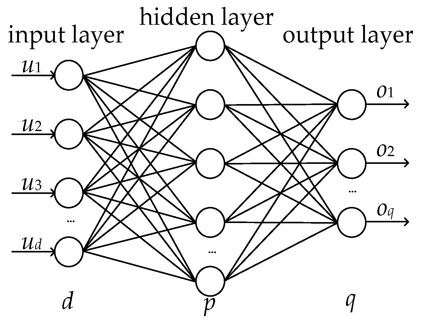
RBFNN is a kind of widely used artificial neural network with strong approximating ability. In general, RBFNN consists of three layers: the input layer, the hidden layer, and the output layer [35]. A multi-input and multi-output RBFNN is displayed as Figure 2, d represents the number of input layers, p represents the number of hidden layers, and q represents the number of output layers.

Figure 2. RBF neural network.

The output of RBFNN [36,37] is

$$\mathit{o}(k)=\mathit{W}\mathsf{\Psi }(\mathit{u}(k))$$

(4)

where u(k) ∈ R^d and o(k) ∈ R^q are called the input vector and output vector of network, respectively, W = [w_pq] ∈ ${\mathbf{R}}^{p\times q}$ is the weight matrix to be turned, Ψ(u(k)) = [Ψ₁(u(k)), …, Ψ_p(u(k))]^T ∈ R^p is the basis function, p is the node number of RBFNN. The basis function is chosen as the following Gaussian function:

$${\Psi }_p(\mathit{u}(k))=\exp (-\frac{‖\mathit{u}(k)-v_p‖}{{\sigma }_p^2})$$

(5)

where v_p∈ R^p is the width and σ_p is the center of RBFNN.

In order to improve the readability, the symbols used in this paper are listed in Table 1 below.

Table 1. Symbols.

Symbol	Meaning
l	The vector consisting of queuing lengths of each phase
$\widehat{\mathit{l}}$	The predicted values of l
g	The vector consisting of green times of each phase
m	The number of phases
d	The number of input layer nodes of the RBFNN
p	The number of hidden layer nodes of the RBFNN
q	The number of output layer nodes of the RBFNN
u	The input vector of RBFNN
o	The output vector of RBFNN
Ψ	The basis function between input and hidden layer
Ψ	The vector consisting of Ψ
w	The weight coefficient between hidden and output layer
W	The vector consisting of w
v	The width matrix of RBFNN
σ	The center of RBFNN
${\mathsf{\Phi }}_{f,L_l,L_g}$	Pseudo partitioned Jacobian matrix (PPJM)
$\Delta {\mathit{G}}_{L_l,L_g}$	The vector consisting of corresponding output and input
y	The vector consisting of the differences between l and $\widehat{\mathit{l}}$
$\widehat{\mathit{y}}$	The desired values of y
α, β	Inertia coefficient, learning rate
a, b	Weight coefficient
e	The vector consisting of the differences between y and $\widehat{\mathit{y}}$
η	Step factor of MFAC
μ	Weighting factor of MFAC
Cbase	The basic cycle used in the intersection
Cmax	The max cycle used in the intersection
ls	The parameter used in the variable cycle algorithm

3. Multi-Phase Traffic Signal Controller Design

3.1. FFDL-MFAC Symmetrical Controller Design

Lemma 1 [38].

Consider nonlinear system (1) satisfying Assumptions 1–2. If $‖\Delta g(k)‖\ne 0$, then there exists a time-varying vector called pseudo partitioned Jacobian matrix ${\mathsf{\Phi }}_{f,L_l,L_g}(k)=[{\mathsf{\Phi }}_1(k),\dots ,{\mathsf{\Phi }}_{L_l+L_g}(k)]\in {\mathbf{R}}^{m\times (m{L}_l+m{L}_g)}$, PPJM for short, such that system (1) can be transformed into the following FFDL data model:

$$\Delta \mathit{l}(k+1)={\mathsf{\Phi }}_{f,L_l,L_g}(k)\Delta {\mathit{G}}_{L_l,L_g}(k)$$

(6)

$$\Delta \mathit{g}(k)=\mathit{g}(k)-\mathit{g}(k-1)$$

(7)

$$\Delta \mathit{l}(k+1)=\mathit{l}(k+1)-\mathit{l}(k)$$

(8)

$${\mathsf{\Phi }}_i(k)=\left[\begin{array}{cccc}{\phi }_{11i}(k)& {\phi }_{12i}(k)& \dots & {\phi }_{1mi}(k)\\ {\phi }_{21i}(k)& {\phi }_{22i}(k)& \dots & {\phi }_{2mi}(k)\\ ⋮& ⋮& \ddots & ⋮\\ {\phi }_{m1i}(k)& {\phi }_{m2i}(k)& \cdots & {\phi }_{mmi}(k)\end{array}\right]\in {\mathbf{R}}^{m\times m}$$

(9)

$$\Delta {\mathit{G}}_{L_l,L_g}(k)=[\Delta {\mathit{l}}^{\mathrm{T}}(k),\dots ,\Delta {\mathit{l}}^{\mathrm{T}}(k-L_l+1),\Delta {\mathit{g}}^{\mathrm{T}}(k),\dots ,\Delta {\mathit{g}}^{\mathrm{T}}(k-L_g+1){]}^{\mathrm{T}}$$

(10)

where f represents the nonlinear function, L_l and L_g represent the control output and input linearization length constant in the FFDL, respectively, Φ_i(k) represents the corresponding sub-square arrays, g(k) and l(k) represent the green times and queuing lengths of each phase in the k-th cycle, respectively, Δl^T(k) = l^T(k) − l^T(k − 1), and Δg^T(k) = g^T(k) − g^T(k − 1).

Note that (6) gives a dynamically linearized data model abound the operational point. Then, the rest of the task is to estimate the PPJM ${\mathsf{\Phi }}_{f,L_l,L_g}$ by traffic data. The following performance index is used to acquire the projection algorithm:

$$J({\mathsf{\Phi }}_{f,L_l,L_g}(k))={‖\Delta \mathit{l}(k)-{\mathsf{\Phi }}_{f,L_l,L_g}(k)\Delta {\mathit{G}}_{L_l,L_g}(k-1)‖}^2+\mu {‖{\mathsf{\Phi }}_{f,L_l,L_g}(k)-{\mathsf{\Phi }}_{f,L_l,L_g}(k-1)‖}^2$$

(11)

Differentiating and simplifying the cost function, one derives Equation (12). Additionally, reset condition (13) are added to improve the estimation ability of (12), where ${\phi }_{ij1}(1)$ is the initial value of ${\phi }_{ij1}(k)$, ${\phi }_{ii1}(1)$ is the initial value of ${\phi }_{ii1}(k)$, and μ > 0, η > 0 are two parameters.

$${\mathsf{\Phi }}_{f,L_l,L_g}(k)={\mathsf{\Phi }}_{f,L_l,L_g}(k-1)+\frac{\eta (\Delta \mathit{l}(k)-{\mathsf{\Phi }}_{f,L_l,L_g}(k-1)\Delta {\mathit{G}}_{L_l,L_g}(k-1))\Delta {\mathit{G}}_{L_l,L_g}^{\mathrm{T}}(k-1)}{\mu +‖\Delta {\mathit{G}}_{L_l,L_g}{(k-1)}^2‖}$$

(12)

$$\begin{array}{l}{\phi }_{ii(L_l+1)}(k)={\phi }_{ii(L_l+1)}(1),if |{\phi }_{ii(L_l+1)}(k)|<b_2 or |{\phi }_{ii(L_l+1)}(k)|>\alpha b_2 or sign({\phi }_{ii(L_l+1)}(k))\ne sign({\phi }_{ii(L_l+1)}(1)),\\ i=1,\dots ,L_l+L_g\\ {\phi }_{ij(L_l+1)}(k)={\phi }_{ij(L_l+1)}(1),if |{\phi }_{ij(L_l+1)}(k)|>b_1 or sign({\phi }_{ij(L_l+1)}(k))\ne sign({\phi }_{ij(L_l+1)}(1)),i,j=1,\dots ,L_l+L_g,i\ne j\end{array}$$

(13)

From Equations (6)–(13), one obtains:

$$\widehat{\mathit{l}}(k+1)=\mathit{l}(k)+{\mathsf{\Phi }}_{f,L_l,L_g}(k)\Delta {\mathit{G}}_{L_l,L_g}(k)$$

(14)

$$g_i(k+1)=b\times {\widehat{l}}_i(k+1)\times (C-m\times y_y)/{\displaystyle \sum _{i=1}^m{\widehat{l}}_i(k+1)}+a\times l_i(k)\times (C-m\times y_y)/{\displaystyle \sum _{i=1}^m{l}_i(k)}$$

(15)

where $\widehat{\mathit{l}}(k)$ represent the estimated queuing lengths of each phase in the k-th cycle, and a > 0, b > 0 satisfying a + b = 1.

Remark 3.

Equations (14) and (15) plays the key role of symmetrical queuing balancing method design. Equation (14) predicts the queuing length in the next cycle based on the FFDL data model with estimated PPJM. Equation (15) calculates the green time via the idea of driving symmetrical flow by balancing the queuing length. The term ${\widehat{l}}_i(k+1)\times (C-m\times y_y)/{\displaystyle \sum _{i=1}^m{\widehat{l}}_i(k+1)}$ gives phase i the effective green time by the ratio of the prediction queuing result in the k + 1-th time instant, while $l_i(k)\times (C-m\times y_y)/{\displaystyle \sum _{i=1}^m{l}_i(k)}$ is the effective green time according to the queuing length of current time instant. The parameters a and b are utilized to coordinates these two terms in case of drastic changes in the signal timing.

Green light time constraint:

Case 1: g_i(k) < g_min

$${\overline{g}}_i=g_{\mathit{min}}$$

Case 2: $g_i>g_{\mathit{min}}$ and ${\displaystyle \sum _{i=1}^m{g}_i>C-g_{\mathit{min}}}$

$${\overline{g}}_i=\max \{g_{\mathit{min}},(C-\Delta t)\times g_i/{\displaystyle \sum _{i=1}^m{g}_i}\}$$

Case 3: ${\displaystyle \sum _{i=1}^m{g}_i}>C-g_{\mathit{min}}$, $g_i>g_{\mathit{min}}$, $g_j<g_{\mathit{min}}$ and the number of g_i is n, the number of g_j is m − n.

$${\overline{g}}_i=\max \{g_{\mathit{min}},(C-\Delta t-(m-n)\times g_i)/{\displaystyle \sum _{i=1}^n{g}_i}\}$$

where g_min, C, and g_i(k) represent the minimum green time, the fixed period duration and the green time in i-th phase of the k-th cycle, respectively, and Δt represents the delay and the sum of the non-green time such as the yellow time.

3.2. RBFNN-Enhanced Controller Design

To further exploit the potential of signal control, a variable cycle algorithm is added in this section. Additionally, the green time assignment in the variable cycle case is presented as follows:

$${\overline{g}}_i(k+1)=b\times {\widehat{l}}_i(k+1)\times (C(k+1)-m\times y_y)/{\displaystyle \sum _{i=1}^m{\widehat{l}}_i(k+1)}+a\times l_i(k)\times (C(k+1)-m\times y_y)/{\displaystyle \sum _{i=1}^m{l}_i(k)}$$

(16)

$$C(k+1)=\mathit{min}\left(C_{base} / \left(1-\left({\displaystyle \sum _{i=1}^m{l}_i(k)} / l_s\right)\right), C_{\mathit{max}}\right)$$

(17)

where ${\overline{g}}_i(k+1)$ ≥ g_min, l_s is a parameter, C_base/C_max is the basic/maximum cycle used in the intersection, and a > 0, b > 0 satisfying a + b = 1.

Remark 4.

Equation (17) gives a variable cycle algorithm. The basic idea is to change the cycle based the saturation of queuing length of each phase. C_base and C_max can be determined by the Webster method or just use the real cycle on the intersection. l_s is a parameter should be the estimated by the historical data, e.g., the max sum of queuing length in the past 3 months. In the simulation, according to the investigation and a trial-and-error method, we chose them as C_base = 100, C_max = 260, l_s = 256.

Now, the following section illustrates the tuning process enhanced by the RBFNN.

From (6), (12), (16), and (17), one obtained Equations (18) and (19).

$$\begin{array}{l}{\overline{g}}_i(k+1)=\frac{b(C(k+1)-m\times y_y)\times {\widehat{l}}_i(k+1)}{{\displaystyle \sum _{i=1}^m{\widehat{l}}_i(k+1)}}+\frac{a(C(k+1)-m\times y_y)\times l_i(k)}{{\displaystyle \sum _{i=1}^m{l}_i(k)}}\\ =\frac{a(C(k+1)-m\times y_y)\times l_i(k)}{{\displaystyle \sum _{i=1}^m{l}_i(k)}}+\frac{b(C(k+1)-m\times y_y)\times l_i(k)+{\overline{\mathsf{\Phi }}}_i(k-1)\Delta {\mathit{G}}_{L_l,L_g}(k)}{{\displaystyle \sum _{i=1}^m{l}_i(k)}+{\displaystyle \sum _{i=1}^m{\overline{\mathsf{\Phi }}}_i(k-1)\times \Delta {\mathit{G}}_{L_l,L_g}(k)}+H(k)}\\ +\frac{b\eta (k)(C(k+1)-m\times y_y)\times (\Delta l_i(k)-{\overline{\mathsf{\Phi }}}_i(k-1)\Delta {\mathit{G}}_{L_l,L_g}(k-1))\Delta {\mathit{G}}_{L_l,L_g}^{\mathrm{T}}(k-1)\Delta {\mathit{G}}_{L_l,L_g}(k)}{(\mu (k)+{‖\Delta {\mathit{G}}_{L_l,L_g}(k-1)‖}^2)\times ({\displaystyle \sum _{i=1}^m{l}_i(k)}+{\displaystyle \sum _{i=1}^m{\overline{\mathsf{\Phi }}}_i(k-1)\times \Delta {\mathit{G}}_{L_l,L_g}(k)}+H(k))}\end{array}$$

(18)

$$H(k)=\frac{\eta (k)({\displaystyle \sum _{i=1}^m\Delta l_i(k)}-{\displaystyle \sum _{i=1}^m{\overline{\mathsf{\Phi }}}_i(k-1)\times \Delta {\mathit{G}}_{L_l,L_g}(k-1)})\Delta {\mathit{G}}_{L_l,L_g}^{\mathrm{T}}(k-1)\Delta {\mathit{G}}_{L_l,L_g}(k)}{\mu (k)+{‖\Delta {\mathit{G}}_{L_l,L_g}(k-1)‖}^2}$$

(19)

and

$${\mathsf{\Phi }}_{f,L_l,L_g}(k-1)=\left[\begin{array}{c}{\overline{\mathsf{\Phi }}}_1(k-1)\\ {\overline{\mathsf{\Phi }}}_2(k-1)\\ {\overline{\mathsf{\Phi }}}_3(k-1)\\ {\overline{\mathsf{\Phi }}}_4(k-1)\end{array}\right]$$

(20)

Define two following error variables for the tuning purpose.

$$y_i(k)=l_i(k)-{\widehat{l}}_i(k)$$

(21)

$$e_i(k)=y_i^{\ast }(k)-y_i(k)$$

(22)

where y_i(k) represents the difference between actual and predicted queuing lengths in i-th phase of the k-th cycle, and y_i^*(k) is the desired value of y_i(k), i = 1, …, m.

$$\begin{array}{l}{u}_1(k)={\displaystyle \sum _{i=1}^m{e}_i(k)}\\ u_2(k)={\displaystyle \sum _{i=1}^m{\displaystyle \sum _{k=1}^k{e}_i(k)}}\\ u_3(k)={\displaystyle \sum _{i=1}^m(e_i}(k)-e_i(k-1))\end{array}$$

(23)

Therefore, the Input vector is: u(k) = [u₁(k), u₂(k), u₃(k)]^T. In the same time, as shown in Equation (5), the hidden layer is: $\mathsf{\Psi }(\mathit{u}(k))=[{\psi }_1(\mathit{u}(k)),\cdots ,{\psi }_p(\mathit{u}(k)){]}^{\mathrm{T}}.$

Additionally, the output vector is:

$$o_q(k)={\displaystyle \sum _{j=1}^p{w}_{jq}{\psi }_j(\mathit{u}(k))}$$

(24)

The connection weights between the hidden layer and the output layer are W. Additionally, W is the vector consisting of w. Define following performance indicator function:

$$M=\frac{1}{2}{\displaystyle \sum _{i=1}^m{e}_i^2}(k)$$

(25)

Search for the negative gradient direction of the coefficient according to Equations (18)–(25), and result is as shown in Equation (26).

$$\begin{array}{l}\Delta \mathit{W}=-\beta \frac{\partial M}{\partial \mathit{W}}+\alpha \Delta \mathit{W}\\ \frac{\partial M}{\partial \mathit{W}}={\displaystyle \sum _{s=1}^m{\displaystyle \sum _{i=1}^m\frac{\partial M}{\partial y_s(k)}\frac{\partial y_s(k)}{\partial g_i(k)}}}\frac{\partial g_i(k)}{\partial o_q(k)}\frac{\partial o_q(k)}{\partial \mathit{W}}\end{array}$$

(26)

Simplifying Equation (26) obtains Equation (27) for updating the weight coefficient of RBFNN.

$$\begin{array}{l}\Delta \mathit{W}=\beta \mathsf{\Psi }(\mathit{u}(k))\mathcal{l}(k)+\alpha \Delta \mathit{W}\\ {\mathcal{l}}_q(k)={\displaystyle \sum _{s=1}^m{\displaystyle \sum _{i=1}^m{e}_s(k)sign(\frac{\partial y_s(k)}{\partial g_i(k)})}}\frac{\partial g_i(k)}{\partial o_q(k)}\\ \mathcal{l}(k)=[{\mathcal{l}}_1(k),{\mathcal{l}}_2(k),\cdot \cdot \cdot {\mathcal{l}}_q(k)]\end{array}$$

(27)

where η(k) = o₁(k), μ(k) = o₂(k). So, q = 2, and Equation (28) can be obtained from the above:

$$\begin{array}{l}\frac{\partial {\overline{g}}_i(k)}{\partial o_1(k)}=\frac{\partial {\overline{g}}_i(k)}{\partial \eta (k)}\\ \frac{\partial {\overline{g}}_i(k)}{\partial o_2(k)}=\frac{\partial {\overline{g}}_i(k)}{\partial \mu (k)} i=1,\dots ,m\end{array}$$

(28)

In summary, the overall design block diagram is given in Figure 3, and the application procedure is expressed by pseudo code, as shown in Algorithm 1.

Figure 3. The design of FFDL-RBFNN.

4. Application Steps of the Proposed Algorithm

Algorithm 1: RBFNN-FFDL algorithm for the intersection with fast-changing traffic flow
Import traci
Input: maximum control cycle number kmax, non-green time yy, minimum green time gmin, α, β; the initial values of l, $\widehat{\mathit{l}}$, g, y, ${\mathsf{\Phi }}_{f,L_l,L_g}$,$\Delta {\mathit{G}}_{L_l,L_g}$, C, W, η, μ, e, v and σ.
1. Initialization: Q(k) = 0;
2. for k = 2 to kmax
	3. The queuing lengths of each phase are obtained through the detectors.
	li(k) = traci.lanearea.getJamLengthVehicle()
	4. If Q(k) < T
		5. $\widehat{\mathit{l}}(k)=\mathit{l}(k-1)+{\mathsf{\Phi }}_{f,L_l,L_g}(k-1)\Delta {\mathit{G}}_{L_l,L_g}(k-1)$, as Formula (14). The queuing lengths of k-period is predicted by the data of (k − 1)-period.
		6. $\mathit{y}(k)=\mathit{l}(k)-\widehat{\mathit{l}}(k)$, as Formula (21). The difference between the actual queuing lengths of k-period and the predicted queuing lengths are calculated.
		7. $\mathit{e}(k)=\mathit{y}*(k)-\mathit{y}(k)$, as the input of RBFNN, as Formulas (22) and (23).
		8. Search for the negative gradient direction of the coefficient, as Formulas (24)–(28), to update weight coefficient W.
		9. Q(k) += 1
	10. End if
	11. Select the η(k) and μ(k) that corresponds to the requirements when e(k) meet the requirements.
	12. $\Delta {\mathit{G}}_{L_l,L_g}(k)=\mathbf{X}(\Delta \mathit{l}(k),\Delta \mathit{l}(k-1),\Delta \mathit{g}(k),\Delta \mathit{g}(k-1))$, X(h) represents a function about h.
	13. ${\mathsf{\Phi }}_{f,L_l,L_g}(k)={\mathsf{\Phi }}_{f,L_l,L_g}(k-1)+{\rm K}(\eta \left(k\right),\mu \left(k\right),l\left(k\right),\Delta {\mathit{G}}_{L_l,L_g}\left(k\right))$, K(t) represents a function about t.
	14. The variable period C(k + 1) can be calculated from Formula (17).
	15. $\widehat{\mathit{l}}(k+1)=\mathit{l}(k)+{\mathsf{\Phi }}_{f,L_l,L_g}(k)\Delta {\mathit{G}}_{L_l,L_g}(k)$, predict the queuing lengths for the next cycle.
	16. $g_i(k+1)=\Lambda (\mathit{l}(k),\widehat{\mathit{l}}(k+1),C(k+1))$, $\Lambda (\theta )$ represents a function about θ, i represents phase.
	17. Set gi(k + 1) to traffic light.
	SET: traci.trafficlight.setPhaseDuration(‘ ‘, g(k + 1))
	18. k = k + 1
19. End for
Traci.simulationStep()

5. Simulation

5.1. Simulation Platform

The simulation was conducted on SUMO (Simulation of Urban Mobility), an open-source microscopic traffic simulation software. It supports the user-defined control algorithm obtaining real-time traffic information. The test was developed by Python using the TraCI (Traffic Control Interface) interface, while controlling the vehicle states and signal light states in real time. It is noteworthy that Algorithm 1 was also presented in the SUMO environment. Thus, one can easily recurrent or transplant the method into the traffic signal controller in the field test. Please see the official website for more details of SUMO.

The simulation intersection is shown in Figure 4 with four phases. There were three lanes in each direction: straight, left turn and right turn, and the roads were set as 600 m, the detectors in each phase were set as 500 m (i.e., the queuing length can be measured completely). The simulation time was 19,800 s.

Figure 4. The intersection of SUMO running interface.

The test platform versions were SUMO 1.15.0 and Python 3.10.0. Additionally, the CPU was 11th Gen Intel(R) Core (TM) i7-11800H @ 2.30GHz.

5.2. Low Traffic Demand

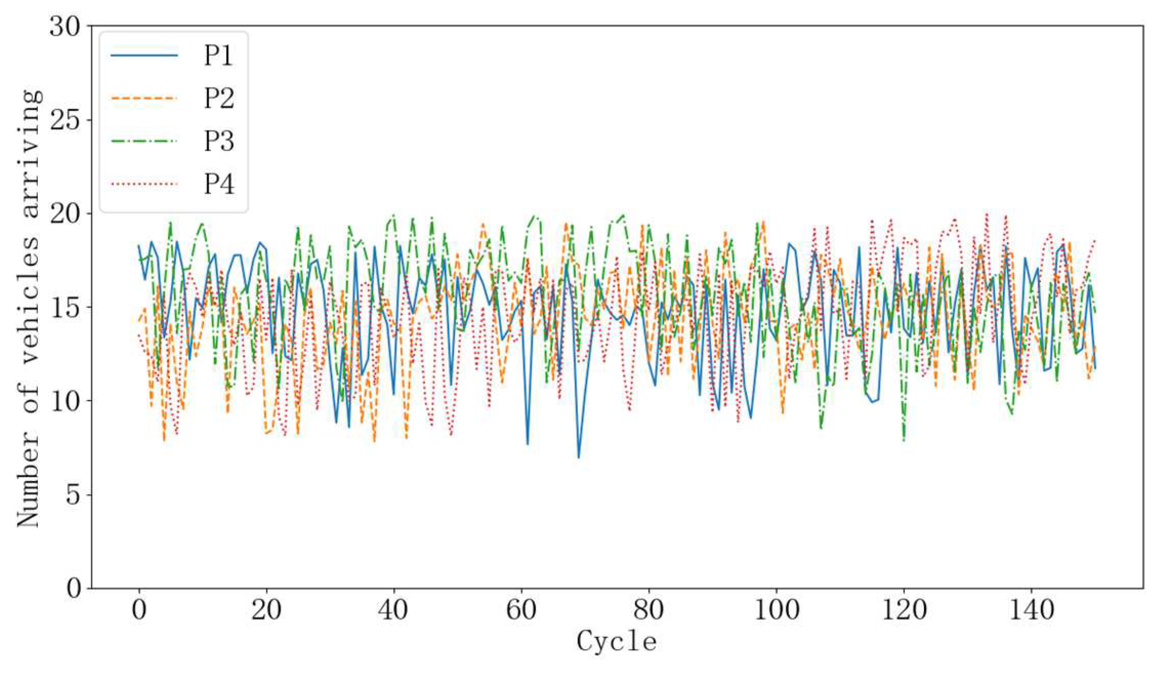
The flow rates of vehicles used in the simulations are shown in Figure 5, which were the actual values with fluctuations in a certain range based on the values in Table 1. The traffic flow of arriving vehicles was subjected to the Formula (29):

$$\tilde{\mathit{n}}(k)=\mathit{n}(k)+\mathbf{U}(-1/25,1/25)$$

(29)

where ñ(k) and n(k) represent the actual flow rates and basic flow rates as Table 2, and U represents a random variable subjecting to the uniform distribution. For example, in the time interval 0–6600 s, the vehicle base arrival rate of Phase 2 was 1/10. So, the actual vehicle arrival rate of this phase was [1/10 − 1/25, 1/10 + 1/25] = [3/50, 7/50], i.e., the number of arrived vehicles was a random number between [6 and 14] for 100 s.

Figure 5. Actual number of vehicles arriving in each phase per cycle under low traffic demand (where P means Phase).

Table 2. Basic vehicle arrival rate under low traffic demand.

Period of Time (s)	Phase
	Phase1	Phase2	Phase3	Phase4
0–6600	1/9	1/10	1/10	1/12
6601–13,200	1/9	1/10	1/11	1/9
13,201–19,800	1/11	1/9	1/10	1/10

(1)

Fixed timing control (FC)

In the fixed time control strategy, the green time and cycle were set to be constants as g₁ = 31, g₂ = 30, g₃ = 29, g₄ = 30, y_y = 3, C = 132, and the cycle number K_f = 150.

(2)

Linear control (LC)

See more details of the control flow diagram in [3]. Based on the cut-and-trial method, parameters were chosen as α₁ = α₂ = α₃ = α₄ = 2; β₁ = β₂ = β₃ = β₄ = 0.1; g_min = 15, g_max = 60.

(3)

Variable-period queuing feedback control (VQF)

In this strategy, the green time for each phase was calculated by the equation $g_i(k)=l_i(k)\times (C-m\times y_y)/{\displaystyle \sum _{i=1}^m{l}_i(k)}$, with parameters g_i(1) = 30, C (1) = 132, y_y = 3, g_min = 15, i = 1, 2, 3, 4.

(4)

FFDL control based on queuing feedback (FFDL-QF)

For comparison purse, FFDL-QF strategy (without the two-layer tuning part) comprises of (6)–(9) and (14)–(15) were used, where g_i(1) = 30, ∆g_i(1) = 1, y_y = 3, C = 132, a = 0.9, b = 0.1, η = 0.01, μ = 0.1, l_i(1) = 0, ∆l_i(1) = 1, $\Delta {\mathit{G}}_{L_l,L_g}(1)=I_{20\times 1}$, ${\mathsf{\Phi }}_{f,L_l,L_g}(1)=I_{4\times 20}$, I is the matrix with element 1, and the cycle number K_F = 150, g_min = 15, i = 1, 2, 3, 4.

(5)

The proposed algorithm control (FFDL-RBFNN)

For the proposed method, the parameters were chosen as g_i(1) = 30, ∆g_i(1) = 1, y_y = 3, C(1) = 132, a = 0.9, b = 0.1, l_i(1) = 0, ∆l_i(1) = 1, y_i(1) = 0, y_i*(1) = 0, ∆y_i(1) = 1, α = 0.75, β = 0.5, $\mathit{W}=0.5\ast I_{5\times 2}$, $\Delta \mathit{W}=O_{5\times 2}$, $\Delta {\mathit{G}}_{L_l,L_g}(1)=I_{20\times 1}$, ${\mathsf{\Phi }}_{f,L_l,L_g}(1)=I_{4\times 20}$, I is the matrix with element 1, O is the matrix with element 0, v_p = [−1, −2, 3, 2, 0], σ_p = 2, g_min = 15, i = 1, 2, 3, 4, and T = 1000.

The simulation results under low traffic demand are shown in Figure 5, Figure 6, Figure 7, Figure 8 and Figure 9 below.

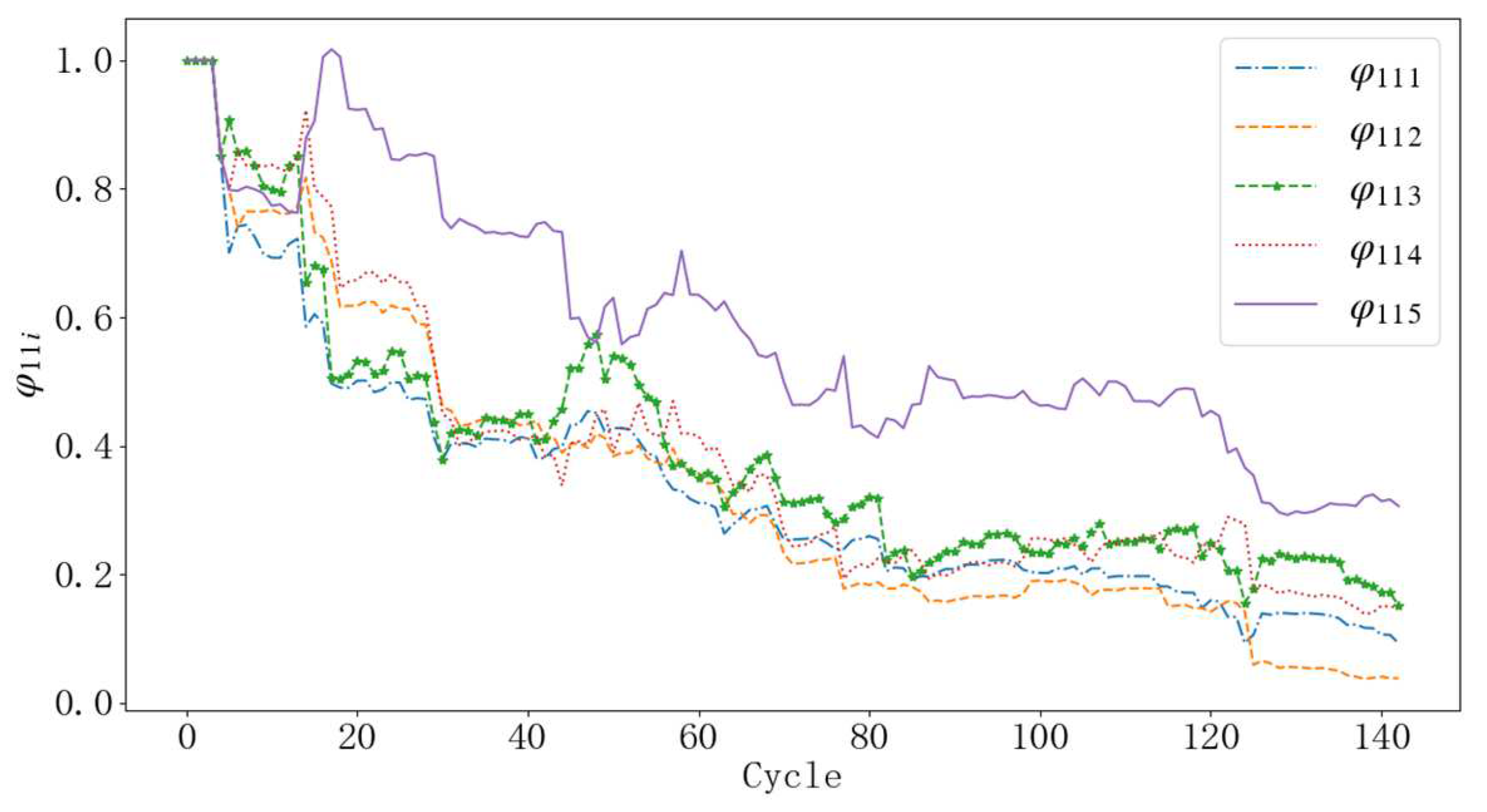
Figure 6. Values of the φ_11i for each cycle under low traffic demand (i = 1, …, 5).

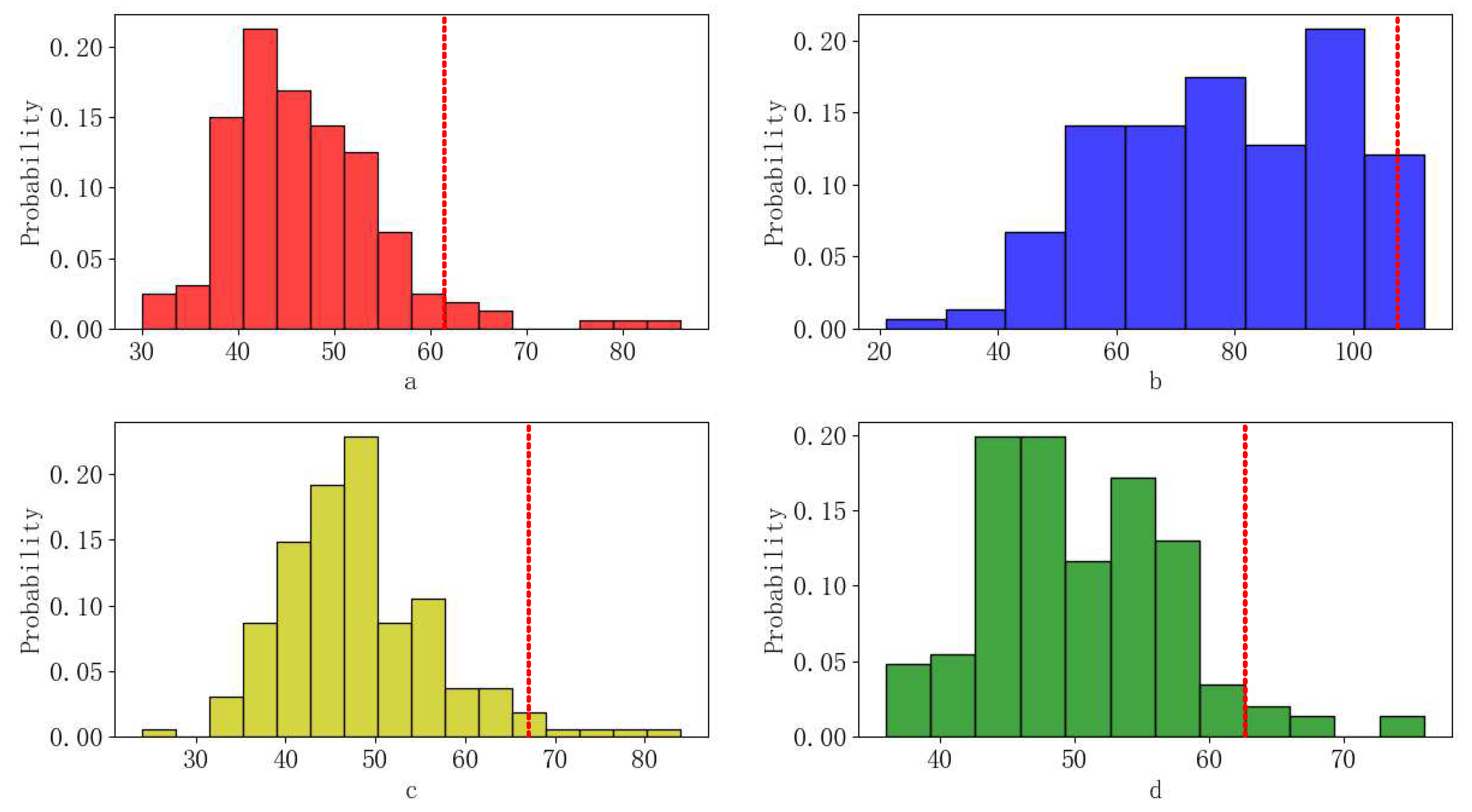
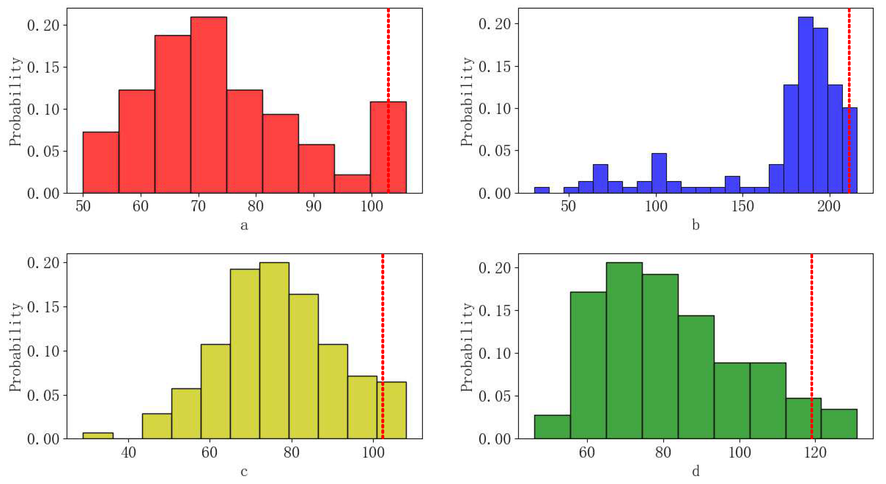
Figure 7. Histograms of green times for each phase under low traffic demand (a)–(d) represent phase 1, phase 2, phase 3, and phase 4, respectively, the red lines indicate the position of the 0.95 quantiles).

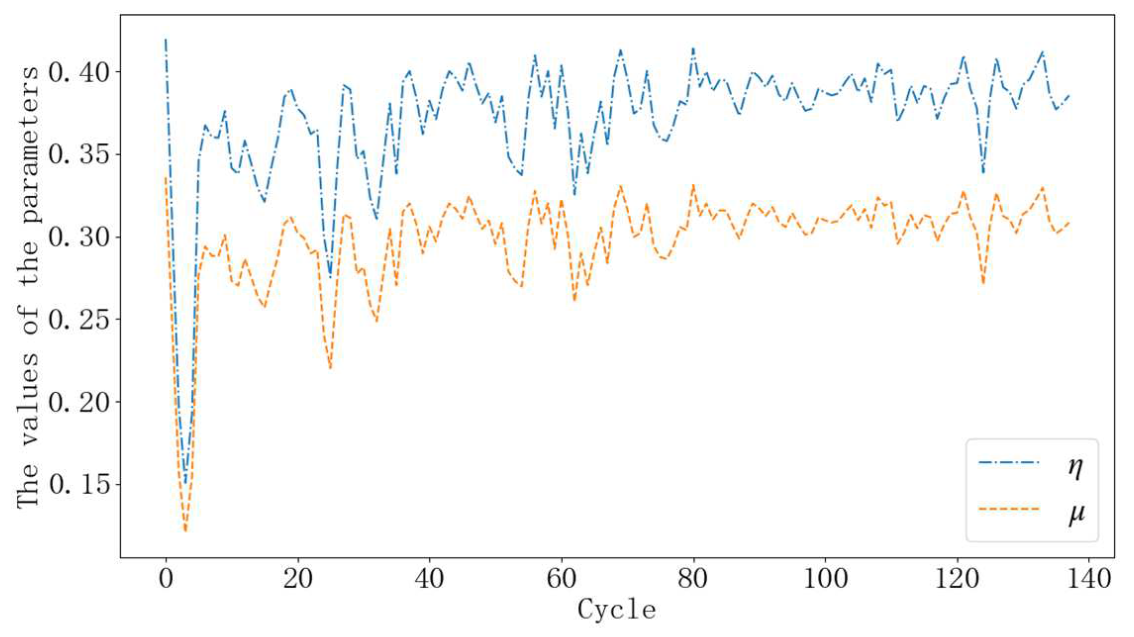
Figure 8. The values of η and μ under low traffic demand.

Figure 9. Histograms of queuing lengths of different control strategies under low traffic demand (a)–(d) represent FC, VQF, FFDL-QF, and FFDL-RBFNN, respectively, the red lines indicate the position of the 0.95 quantiles).

The dimension of ${\mathsf{\Phi }}_{f,L_l,L_g}$ in the calculation process was 4 × 20, consisting of five matrices whose dimensions were 4 × 4. To show the estimating process and avoid the overlap, five elements φ₁₁₁, φ₁₁₂, φ₁₁₃, φ₁₁₄, and φ₁₁₅ (i.e., the elements in the first row and first column of Φ₁(k) − Φ₅(k)) were selected for drawing in Figure 6.

Figure 7 shows the histograms of green times for each phase, Figure 8 shows the values of η and μ under low traffic demand, and Figure 9 shows the histograms of the sum of the maximum queuing lengths of the four phases in each cycle for the different control strategies under low traffic demand.

Observing Figure 9 and Table 3, it can be seen that the queuing lengths and time loss in FC were much longer in this random traffic flow. FFDL-QF and VQF (with 162 cycles running) showed better performance in turn. Finally, the proposed FFDL-RBFNN (with 163 cycles running) had an optimal control effect with shortest average queuing lengths of each cycle (42.22% less than the FC) and less average time loss of vehicles (31.21% less than the FC) under low traffic demand.

Table 3. The values of queuing lengths and time loss of different control strategies under low traffic demand.

Control Strategies	FC	LC	FFDL-QF	VQF	FFDL-RBFNN	Improvement of FFDL-RBFNN Compared with FC
The average queuing lengths of each cycle (veh/cycle)	78.81	\	48.58	47.97(162 *)	45.54(163 *)	42.22%
Average time loss of vehicles (s/veh)	93.41	65.39	68.01	65.53	64.26	31.21%

Note: * means the number of cycles. In the LC design, it does not define a strict cycle concept, so the queuing lengths of each cycle are omitted in the table.

5.3. High Traffic Demand

Table 4 shows the basic vehicle arrival rate under high traffic demand. In the high demand case, the traffic flow still followed Equation (29), while the base arriving rate was increased. Figure 10 shows the actual values with fluctuations in the certain range [−1/25, 1/25], which were used to simulate traffic uncertainty in the real system.

Table 4. Basic vehicle arrival rate under high traffic demand.

Period of Time (s)	Phase
	Phase1	Phase2	Phase3	Phase4
0–6600	1/7.8	1/9	1/6	1/7
6601–13,200	1/7.8	1/7	1/6.7	1/9
13,201–19,800	1/7.5	1/7.7	1/7	1/7

Figure 10. Actual number of vehicles arriving in each phase per cycle under high traffic demand.

(1)

Fixed timing control (FC)

In the high demand case, after ten times tests, we manually found the following relative good signal timing: g₁ = 29, g₂ = 28, g₃ = 34, g₄ = 29, y_y = 3, C = 132, and the cycle number K_f = 150.

(2)

Linear control (LC)

Parameters were the same as the low traffic demand case.

(3)

Variable-period queuing feedback control (VQF)

Parameters were the same as the low traffic demand case.

(4)

FFDL control based on queuing feedback (FFDL-QF)

Parameters were the same as the low traffic demand case.

(5)

The proposed algorithm control (FFDL-RBFNN)

Parameters were the same as the low traffic demand case.

Figure 10 represents actual number of vehicles arriving in each phase per cycle under high traffic demand. Figure 11 shows the changes in the values of φ_11L. Figure 12 depicts the histograms of green times for four phases in each cycle. Figure 13 shows the values of η and μ under high traffic demand. Additionally, Figure 14 shows the histograms of queuing lengths of each cycle of different control strategies under high traffic demand.

Figure 11. Values of the φ_11i for each cycle under high traffic demand (I = 1, …, 5).

Figure 12. Histograms of green times for each phase under high traffic demand (a)–(d) represent phase 1, phase 2, phase 3, and phase 4, respectively, the red lines indicate the position of the 0.95 quantiles).

Figure 13. The values of η and μ under high traffic demand.

Figure 14. Histograms of queuing lengths of different control strategies under high traffic demand (a)–(d) represent FC, VQF, FFDL-QF, and FFDL-RBFNN, respectively, the red lines indicate the position of the 0.95 quantiles).

The result is summarized in Table 5. In this case, FC performed poorly against high demand and fast-changing flow. This usually happened if the signal time was not adjusted according to the change of the area traffic flow after a long time. FFDL-QF and VQF improved a certain level compared with FC, but there still was room to promote. Observing the results in Table 5 and Table 3, it can be seen that LC was effective under low traffic demand. However, it did not perform well under high traffic demand. The main reason for this was that it was designed based on the simplified linear relationship of each phase, and only analyzed under on the unsaturated condition (note that the high demand case may cause an oversaturated condition). The proposed FFDL-RBFNN produced the shortest average queuing lengths of each cycle (58.00% less than the FC) and less average time loss of vehicles (54.78% less than FC), which showed its superiority in a high demand fast-changing traffic flow. In addition, one may also notice that the cycle number of FFDL-RBFNN was 141 (original K_f = 150), which indicates the cycle tended to increase in a high demand case.

Table 5. The values of queuing lengths and time loss of different control strategies under high traffic demand.

Control Strategies	FC	LC	FFDL-QF	VQF	FFDL-RBFNN	Improvement of FFDL-RBFNN Compared with FC
The average queuing lengths of each cycle (veh/cycle)	173.63	\	79.80	76.77(140 *)	72.92(141 *)	58.00%
Average time loss of vehicles (s/veh)	208.12	298.20	102.65	97.39	94.11	54.78%

Note: * means the number of cycles. Like the low traffic demand case, the average queuing lengths of each cycle with LC was omitted in the table.

6. Conclusions

In this paper, a novel MFAC-based symmetrical signal timing design was proposed by combining FFDL and RBFNN. To treat with fast-changing traffic flow in the real world, a two-layer tuning framework was designed, with BRFNN in the first layer continuously accelerating the PPJM estimation process in the second layer. Then, the variable cycle algorithm was further introduced to explore the possibility of single intersection signal control. In order to draw as close as possible to the real traffic flow, this paper set up two simulation scenarios: low traffic demand and high traffic demand superposed with fast-changing random traffic flow. Simulation tests on the SUMO showed that the proposed method outperformed the other four chosen control strategies (FC, LC, FFDL-QF, and VQF).

However, there were still some limitations. This study did not analyze the impact of buses, non-motor vehicles, and pedestrians on traffic flow in detail, which can be added to traffic control for specific analysis in the future. Additionally, the future work included two directions. Firstly, the two-layer tuning frame should be extended from a single intersection to a multi-intersection region. Secondly, an algorithm choosing the initial parameters can be developed. As a priority, the research group is making an attempt to apply the proposed method to real intersection signal control systems.

References

- Wu, N.; Li, D.W.; Xi, Y.G. Distributed Weighted Balanced Control of Traffic Signals for Urban Traffic Congestion. IEEE Trans. Intell. Transp. Syst. 2019, 20, 3710–3720. [Google Scholar] [CrossRef]
- Čubranić-Dobrodolac, M.; Švadlenka, L.; Čičević, S. A bee colony optimization (BCO) and type-2 fuzzy approach to measuring the impact of speed perception on motor vehicle crash involvement. Soft. Comput. 2022, 26, 4463–4486. [Google Scholar] [CrossRef]
- Dunne, M.C.; Potts, R.B. Algorithm for Traffic Control. Oper. Res. 1964, 12, 870–881. [Google Scholar] [CrossRef]
- Pascale, A.; Lam, H.T.; Nair, R. Characterization of Network Traffic Processes Under Adaptive Traffic Control Systems. Transp. Res. Procedia 2015, 9, 205–224. [Google Scholar] [CrossRef]
- Robertson, D.I.; Bretherton, R.D. Optimizing Networks of Traffic Signals in Real Time—The SCOOT Method. IEEE Trans. Veh. Technol. 1991, 40, 11–15. [Google Scholar] [CrossRef]
- Jin, J.; Ma, X.; Kosonen, I. An intelligent control system for traffic lights with simulation-based evaluation. Control. Eng. Pract. 2017, 58, 24–33. [Google Scholar] [CrossRef]
- Kenan, M.; Nezir, A.; Alper, Y. A Data Driven Approach to Forecasting Traffic Speed Classes Using Extreme Gradient Boosting Algorithm and Graph Theory. Phys. A Stat. Mech. Its Appl. 2023, 620, 128738. [Google Scholar]
- Ye, B.L.; Wu, W.M.; Ruan, K.Y. A survey of model predictive control methods for traffic signal control. IEEE CAA J. Autom. Sin. 2019, 6, 623–640. [Google Scholar] [CrossRef]
- Huang, Y.S.; Weng, Y.S.; Wu, W.M. Control strategies for solving the problem of traffic congestion. IET Intell. Transp. Syst. 2016, 10, 642–648. [Google Scholar] [CrossRef]
- Celtek, S.; Durdu, A.; Alı, M. Real-time traffic signal control with swarm optimization methods. Measurement 2020, 166, 108206. [Google Scholar] [CrossRef]
- Yuan, T.C.; Faisal, A.; Zhang, Y.H.; Petros, A.I. Evaluation of Integrated Variable Speed Limit and Lane Change Control for Highway Traffic Flow. IFAC Pap. 2021, 54, 107–113. [Google Scholar] [CrossRef]
- Baldi, S.; Michailidis, L.; Ntampasi, V. A Simulation-Based Traffic Signal Control for Congested Urban Traffic Networks. Transp. Sci. 2019, 53, 6–20. [Google Scholar] [CrossRef]
- Wang, H.; Zhu, M.X.; Hong, W.S. Optimizing Signal Timing Control for Large Urban Traffic Networks Using an Adaptive Linear Quadratic Regulator Control Strategy. IEEE Trans. Intell. Transp. Syst. 2022, 23, 333–343. [Google Scholar] [CrossRef]
- Gao, P.; Yang, Z.S. Regional Traffic Control Evaluation Based on Genetic Neural Network. J. Beijing Univ. Technol. 2010, 36, 490–494. [Google Scholar]
- Molyneaux, N.; Scarinci, R.; Bierlaire, M. Design and analysis of control strategies for pedestrian flows. Transportation 2021, 48, 1767–1807. [Google Scholar] [CrossRef]
- Zhang, Y.; Zhang, Y.C.; Su, R. Pedestrian-Safety-Aware Traffic Light Control Strategy for Urban Traffic Congestion Alleviation. IEEE Trans. Intell. Transp. Syst. 2021, 22, 178–193. [Google Scholar] [CrossRef]
- Hou, Z.S.; Wang, Z. From model-based control to data-driven control: Survey, classification and perspective. Inf. Sci. 2013, 235, 3–35. [Google Scholar] [CrossRef]
- Hou, Z.S.; Jin, S.T. Data-driven model-free adaptive control for a class of MIMO nonlinear discrete-time systems. IEEE Trans. Neural Netw. 2011, 22, 2173–2188. [Google Scholar]
- Hou, Z.S.; Chi, R.H.; Gao, H.J. An Overview of Dynamic-Linearization-Based Data-Driven Control and Application. IEEE Trans. Ind. Electron. 2017, 64, 4076–4090. [Google Scholar] [CrossRef]
- Hou, Z.S.; Zhu, Y.M. Controller-Dynamic-Linearizati- on-Based Model Free Adaptive Control for Discrete-Time Nonlinear Systems. IEEE Trans. Ind. Inform. 2013, 9, 2301–2309. [Google Scholar] [CrossRef]
- Xiong, S.S.; Hou, Z.S. Model-Free Adaptive Control for Unknown MIMO Nonaffine Nonlinear Discrete-Time Systems With Experimental Validation. IEEE Trans. Neural Netw. Learn. Syst. 2022, 33, 1727–1739. [Google Scholar] [CrossRef] [PubMed]
- Feng, J.; Song, W.Z.; Zhang, H.G. Data-Driven Robust Iterative Learning Consensus Tracking Control for MIMO Multiagent Systems Under Fixed and Iteration-Switching Topologies. IEEE Trans. Syst. Man Cybern. Syst. 2022, 52, 1331–1344. [Google Scholar] [CrossRef]
- Xue, G.; Liu, Y.J.; Shi, Z.J. Research on Trajectory Tracking Control of Underwater Vehicle Manipulator System Based on Model-Free Adaptive Control Method. J. Mar. Sci. Eng. 2022, 10, 652. [Google Scholar] [CrossRef]
- Zhang, Z.W.; Jin, S.T.; Liu, G.F. Model-Free Adaptive Direct Torque Control for the Speed Regulation of Asynchronous Motors. Processes 2020, 8, 333. [Google Scholar] [CrossRef]
- Jiang, Q.Q.; Li, Y.; Liao, Y.L. Information fusion model-free adaptive control algorithm and unmanned surface vehicle heading control. Appl. Ocean. Res. 2019, 90, 101851. [Google Scholar] [CrossRef]
- Liao, Y.L.; Du, T.P.; Jiang, Q.Q. Model-free adaptive control method with variable forgetting factor for unmanned surface vehicle control. Appl. Ocean. Res. 2019, 93, 101945. [Google Scholar] [CrossRef]
- Wang, Y.Y.; Liu, L.F.; Yuan, M.X. A New Model-free Robust Adaptive Control of Cable-driven Robots. Int. J. Control Autom. Syst. 2021, 19, 3209–3222. [Google Scholar] [CrossRef]
- Ren, Y.; Hou, Z.S. Robust mode-free adaptive iterative learning formation for unknown heterogeneous non-linear multi-agent systems. IET Control. Theory Appl. 2020, 14, 654–663. [Google Scholar] [CrossRef]
- Hou, Z.S.; Lei, T. Constrained Model Free Adaptive Predictive Perimeter Control and Route Guidance for Multi-Region Urban Traffic Systems. IEEE Trans. Intell. Transp. Syst. 2022, 23, 912–924. [Google Scholar] [CrossRef]
- Ren, Y.; Hou, Z.S.; Sirmatel, I.I. Data driven model free adaptive iterative learning perimeter control for large-scale urban road networks. Transp. Res. Part C Emerg. Technol. 2020, 115, 102618. [Google Scholar] [CrossRef]
- Lei, T.; Hou, Z.S.; Ren, Y. Data-Driven Model Free Adaptive Perimeter Control for Multi-Region Urban Traffic Networks With Route Choice. IEEE Trans. Intell. Transp. Syst. 2020, 21, 2894–2905. [Google Scholar] [CrossRef]
- Cui, X. Model Free Adaptive Control of Multi-Agent Systems and It’s Applications to Coordinated Signal Control of Intersections. Master’s Thesis, Beijing Jiaotong University, Beijing, China, 2015. [Google Scholar]
- Li, D.; De Schutter, B. Distributed Model-Free Adaptive Predictive Control for Urban Traffic Networks. IEEE Trans. Control. Syst. Technol. 2022, 30, 180–192. [Google Scholar] [CrossRef]
- Li, D.; Hou, Z.S. Data-driven urban traffic model-free adaptive iterative learning control with traffic data dropout compensation. IET Control. Theory Appl. 2021, 15, 1533–1544. [Google Scholar] [CrossRef]
- Han, H.G.; Ma, M.L.; Qiao, J.F. Accelerated gradient algorithm for RBF neural network. Neurocomputing 2021, 441, 237–247. [Google Scholar] [CrossRef]
- Xiong, S.S.; Hou, Z.S. Data-Driven Formation Control for Unknown MIMO Nonlinear Discrete-Time Multi-Agent Systems With Sensor Fault. IEEE Trans. Neural. Netw. Learn Syst. 2022, 33, 7728–7742. [Google Scholar] [CrossRef] [PubMed]
- Zhu, Y.M.; Hou, Z.S.; Qian, F. Dual RBFNNs-Based Model-Free Adaptive Control With Aspen HYSYS Simulation. IEEE Trans. Neural. Netw. Learn Syst. 2017, 28, 759–765. [Google Scholar] [CrossRef]
- Hou, Z.S.; Jin, S.T. Model Free Adaptive Control Theory and Applications’; CRC Press, Taylor and Francis Group: Boca Raton, FL, USA, 2013; pp. 69–71. [Google Scholar]
Disclaimer/Publisher’s Note: The statements, opinions and data contained in all publications are solely those of the individual author(s) and contributor(s) and not of MDPI and/or the editor(s). MDPI and/or the editor(s) disclaim responsibility for any injury to people or property resulting from any ideas, methods, instructions or products referred to in the content. |
© 2023 by the authors. Licensee MDPI, Basel, Switzerland. This article is an open access article distributed under the terms and conditions of the Creative Commons Attribution (CC BY) license (https://creativecommons.org/licenses/by/4.0/).