
Temperature Curve of Reflow Furnace Based on Newton’s Law of Cooling

Abstract
:1. Introduction
2. Preparation and Establishment of the Model
2.1. Differential Model of Temperature Change in Welding Area
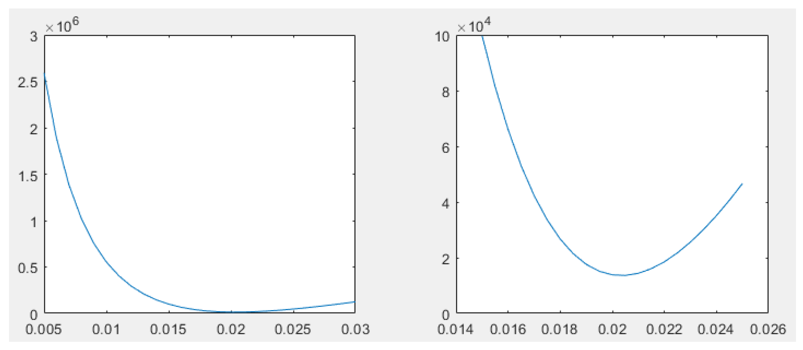
2.2. Determining Coefficient K Using Trial Solution
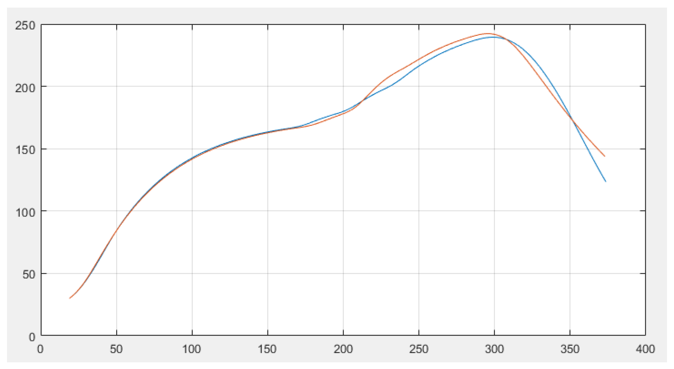
3. Feasibility Test of the Model
4. Solutions to Common Problems in Several Industries
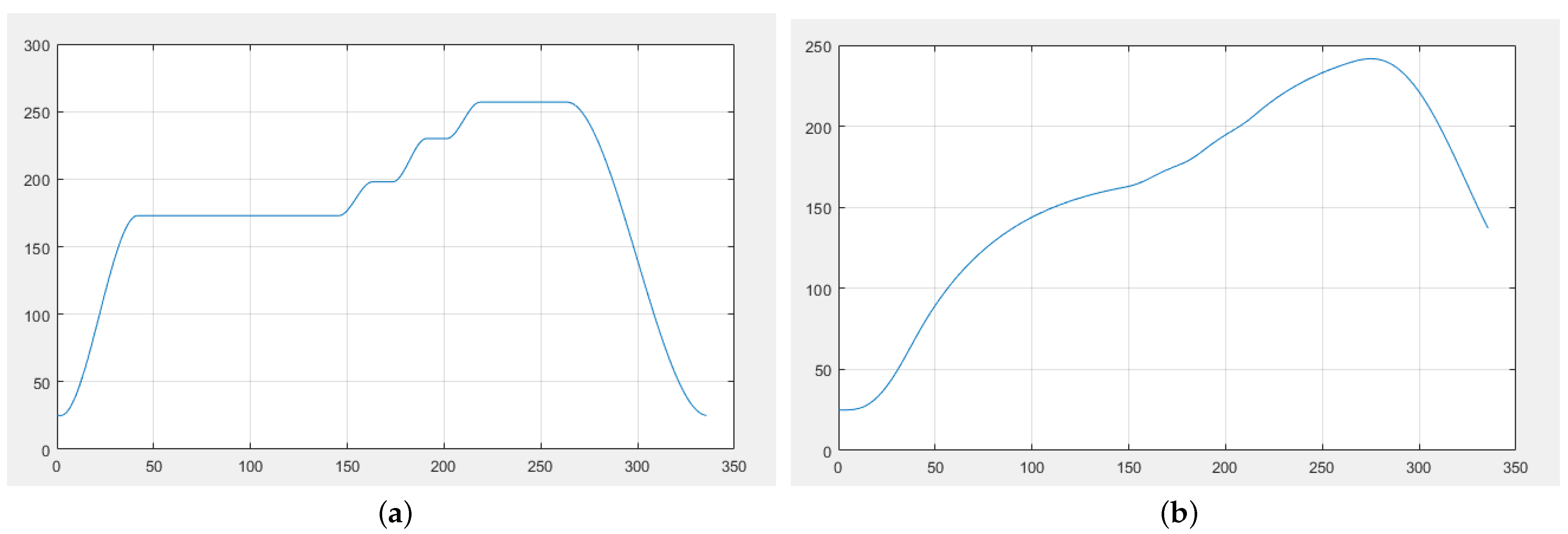
4.1. Drawing Furnace Temperature Curves in Different Temperature Environments
4.2. Optimization of Furnace Speed
- The temperature rising slope must not exceed 3.
- The temperature drop slope must not exceed 3.
- The time for the temperature to rise from 150 C to 190 C must be between 60 s and 120 s.
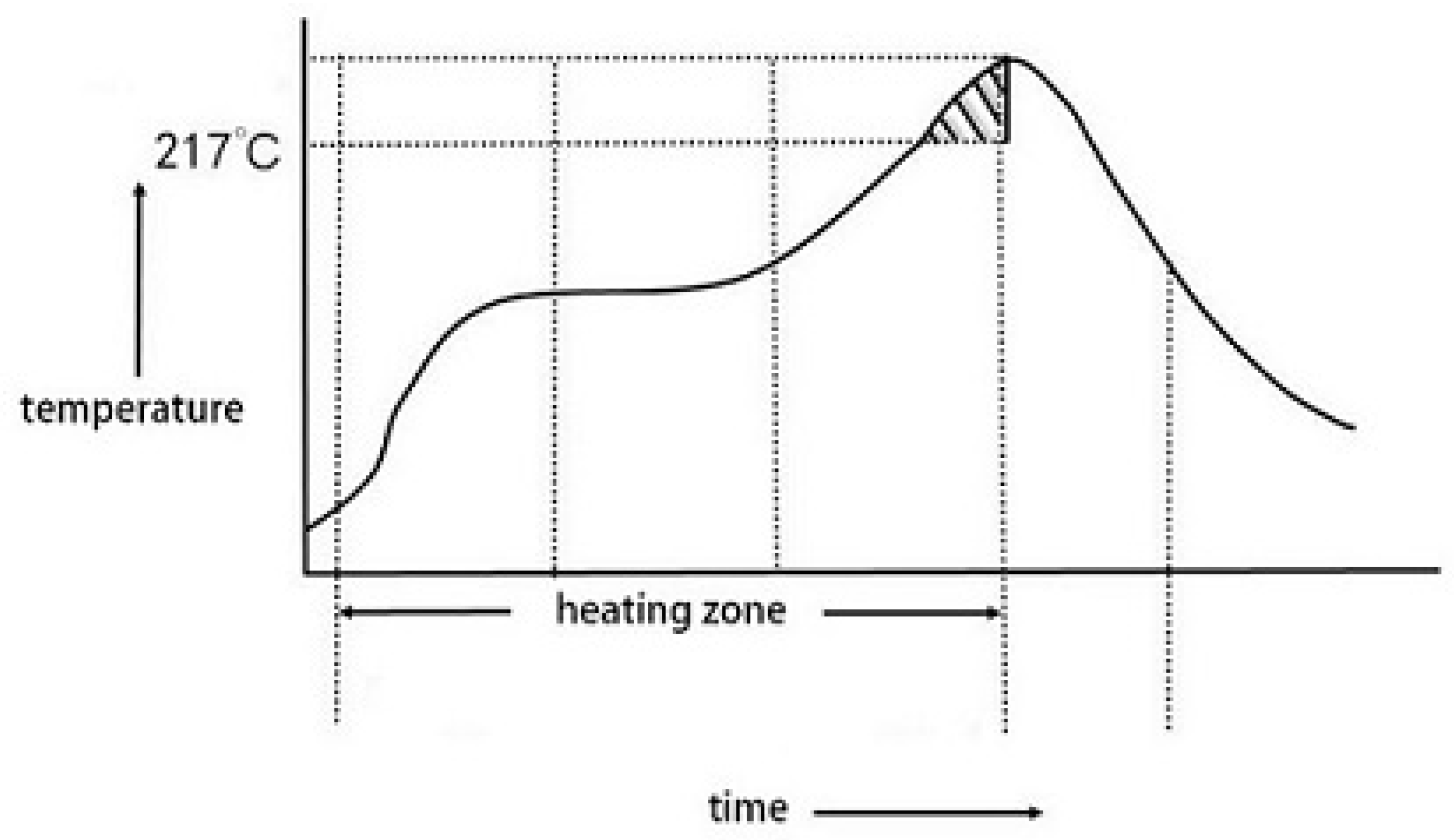
- The temperature above 217 C must be maintained for 40 s to 90 s.
- The highest temperature should be between 240 C and 250 C.
- .
- All satisfied of t compose interval , which satisfies .
- In all ascending segments, all t of meeting the requirements compose the interval of , which satisfies .
- Finally, .
4.3. Peak Temperature Coverage Problem
4.4. Symmetry of Peak Temperature Image
5. Summary
Author Contributions
Funding
Institutional Review Board Statement
Informed Consent Statement
Data Availability Statement
Acknowledgments
Conflicts of Interest
References
- Tang, Z.; Xie, B.; Liang, G. Control analysis of reflow furnace temperature curve. Electron. Qual. 2020, 15–19. [Google Scholar]
- Yao, X. Effect of plate feeding interval on furnace temperature curve. Shandong Ind. Technol. 2015, 271–272. [Google Scholar]
- Gong, Y. Study on temperature curve optimization of reflow welding furnace. Hot Work. Technol. 2013, 42, 187–190. [Google Scholar]
- Jun, F.; Ying, X.; Zeng, Y. Observe the temperature curve for solidification from high-speed video image. J. Therm. Anal. Calorim. 2021, 146, 1–5. [Google Scholar]
- Fradette, J. Real, Vacuum Furnace Temperature Measurement. Ind. Heat. 2015, 83, 52–59. [Google Scholar]
- Kurhade, A.; Rao, T.; Mathew, V. Effect of thermal conductivity of substrate board for temperature control of electronic components: A numerical study. Int. J. Mod. Phys. C 2021, 32, 1–12. [Google Scholar] [CrossRef]
- Li, H.; Li, R.; Wu, F. A New Control Performance Evaluation Based on LQG Benchmark for the Heating Furnace Temperature Control System. Processes 2020, 8, 1428. [Google Scholar] [CrossRef]
- Su, H.; Shi, J.; Ji, H. Investigating on the Iconic Gas Compositions Produced by Low-Temperature Heating Cotton. Symmetry 2020, 12, 883. [Google Scholar] [CrossRef]
- Yang, H.; Zou, L.; Song, Z.; Wang, X. Identification of the Ignition Point of High Voltage Cable Trenches Based on Ceiling Temperature Distribution. Symmetry 2022, 14, 1417. [Google Scholar] [CrossRef]
- Ahmad, I.; Jalil, A.; Ullah, A. Some new exact solutions of (4+1)-dimensional Davey-Stewartson-Kadomtsev-Petviashvili equation. Results Phys. 2023, 45, 106240. [Google Scholar] [CrossRef]
- Ahmad, S.; Saifullah, S.; Khan, A. Resonance, fusion and fission dynamics of bifurcation solitons and hybrid rogue wave structures of Sawada–Kotera equation. Commun. Nonlinear Sci. Numer. Simul. 2023, 119, 107117. [Google Scholar] [CrossRef]
- Alharbi, K.A.M.; Ullah, A. Ikramullah, Impact of viscous dissipation and coriolis effects in heat and mass transfer analysis of the 3D non-Newtonian fluid flow. Case Stud. Therm. Eng. 2022, 37, 102289. [Google Scholar] [CrossRef]
- Shah, Z.; Kumam, P.; Ullah, A. Mesoscopic Simulation for Magnetized Nanofluid Flow within a Permeable 3D Tank. IEEE Access 2021, 9, 135234–135244. [Google Scholar] [CrossRef]
- Naowarat, S.; Saifullah, S.; Ahmad, S. Periodic, Singular and Dark Solitons of a Generalized Geophysical KdV Equation by Using the Tanh-Coth Method. Symmetry 2023, 15, 135. [Google Scholar] [CrossRef]
- Khan, S.; Selim, M.M.; Khan, A. On the Analysis of the Non-Newtonian Fluid Flow Past a Stretching/Shrinking Permeable Surface with Heat and Mass Transfer. Coatings 2021, 11, 566. [Google Scholar] [CrossRef]
- Ullah, A.; Ikramullah; Selim, M.M. A Magnetite–Water-Based Nanofluid Three-Dimensional Thin Film Flow on an Inclined Rotating Surface with Non-Linear Thermal Radiations and Couple Stress Effects. Energies 2021, 14, 5531. [Google Scholar] [CrossRef]
- Ma, H. Study on Prediction and Optimization of Furnace Temperature Curve Based on Temperature Change Model. J. Phys. Conf. Ser. 2021, 1985, 012045. [Google Scholar] [CrossRef]
- Wang, X.; Sun, P.; Bai, H. Control model of Furnace Temperature Curve. J. Phys. Conf. Ser. 2021, 1903, 012030. [Google Scholar] [CrossRef]
- Febriardy, E.; Sutanto; Abimanyu, A. Development of PID-based furnace temperature control system for zirconium calcination. J. Phys. Conf. Ser. 2020, 1436, 012120. [Google Scholar] [CrossRef]
- Qiao, Y.; Zi, Y.; Song, Y. Research on Furnace Temperature Curve Based on Heat Convection and Heat Radiation. E3S Web Conf. 2021, 233, 04004. [Google Scholar]
- Zhang, J.; Jing, Y.; Chao, Y. Research on Furnace Temperature Curve. J. Phys. Conf. Ser. 2021, 2012, 012091. [Google Scholar] [CrossRef]
- Chen, H.; Luo, H.; Wu, S. Optimization of Furnace Temperature Curve Based on GA. IOP Conf. Ser. Earth Environ. Sci. 2021, 769, 1–23. [Google Scholar] [CrossRef]
- Cheng, Y.C. Optimization and simulation of furnace temperature curve based on heat. J. Phys. Conf. Ser. 2021, 1948, 012230. [Google Scholar]
- Zhao, J.; Dan, Q. Mathematical Modeling and Mathematical Experiment; Higher Education Press: Beijing, China, 2014. [Google Scholar]
- Li, Q.; Wang, N.; Yi, D. Numerical Analysis; Tsinghua University Press: Beijing, China, 2008. [Google Scholar]


| Construction Method of | |
|---|---|
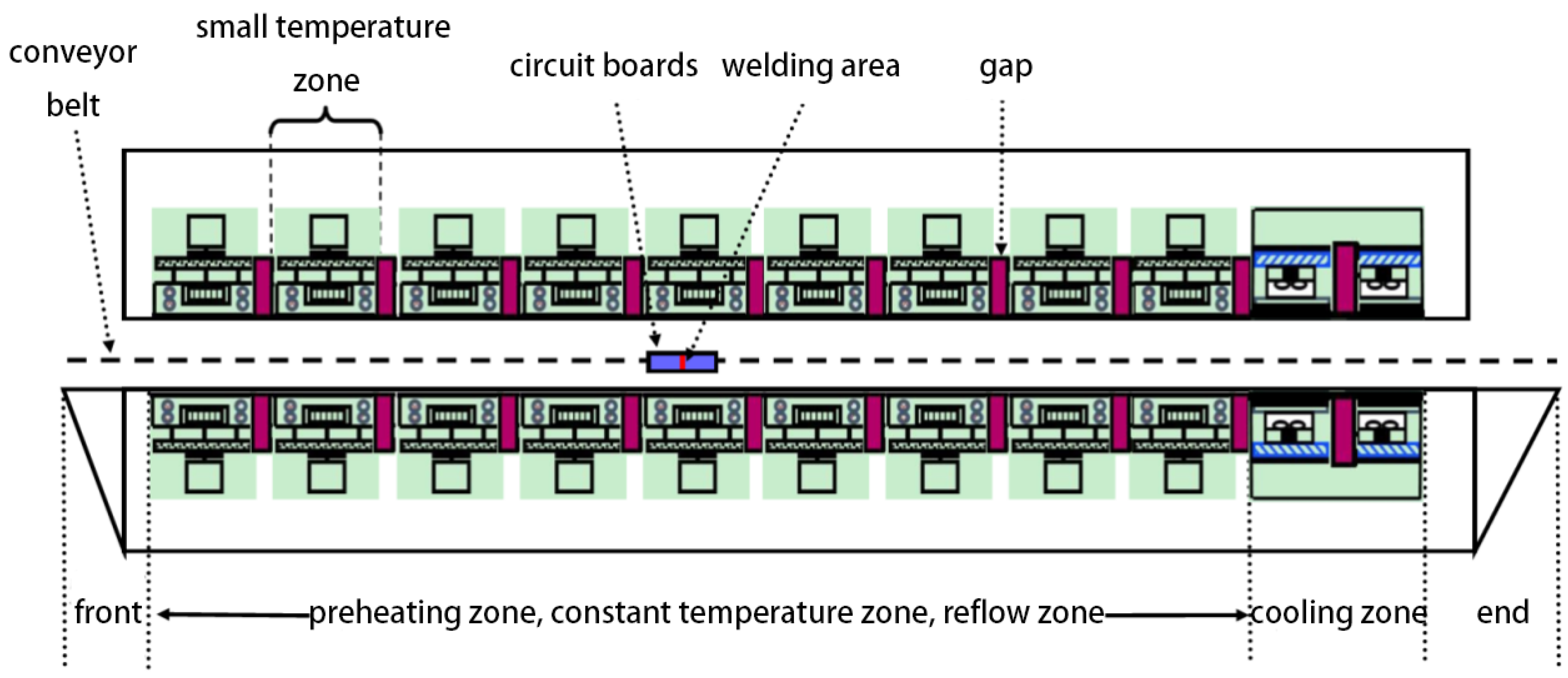
| Step 1 | For a small temperature area, its temperature is , and we set the midpoint of the small temperature range as ; then, we intercept a small neighborhood centered on this point. The figures of in this neighborhood are defined as . |
| Step 2 | For two adjacent and small temperature zones a and b, and the gap between adjacent temperature zones, and for each small temperature zone, we choose the middle point and its neighborhood as in step 1, and respectively record them as and . According to and , for interval , we can carry out cubic interpolation to obtain temperature function in this interval. |
| Step 3 | Generally speaking, in a reflow oven, the set temperature of small temperature zone 1 is quite different from the temperature at the beginning of the furnace front area, but in order to conform to reality, the temperature change should be slow and continuous. We take the distance from the beginning of the furnace front area to the end of small temperature zone 1 as the buffer distance of the temperature change and record it as . In this interval, according to the given temperature at both ends, is obtained with the cubic interpolation method. |
| Step 4 | In the same way as in step 3, because the set temperature of small temperature zone 10 and small temperature zone 11 is the same as the room temperature, the distance from the end of small temperature zone 9 to the end of the rear furnace zone is taken as the buffer zone of temperature change and is recorded as Temperature is obtained by means of cubic interpolation according to the given temperature at both ends. At the same time, |
| Construction Method of | |
|---|---|
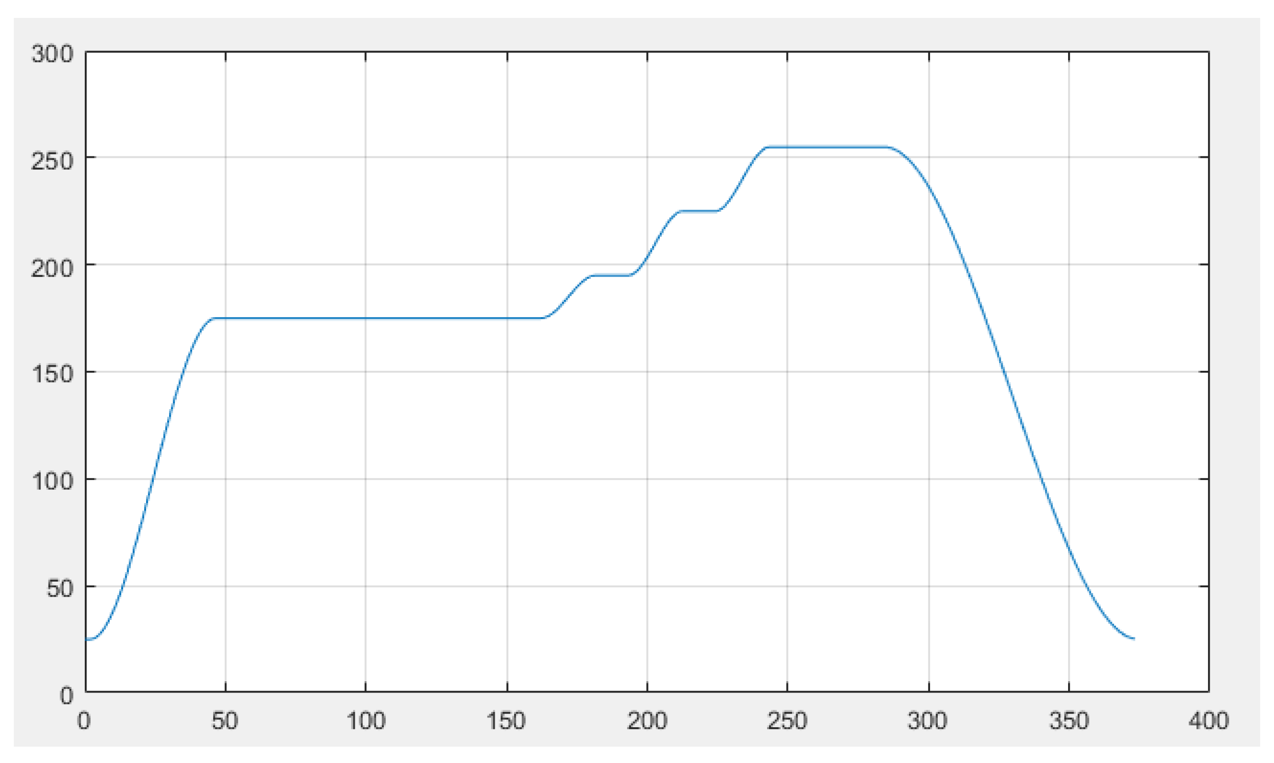
| Step 1 | The set temperature of small temperature zones 1~5 is 175 C; small temperature zone 1 is affected by the area in front of the furnace, and small temperature zone 5 is affected by small temperature zone 6, so we define function in interval . According to the given speed, , we convert interval into the corresponding interval. We make the value of function in the interval be equal to 175 C. Similarly, for small temperature zone 8 and small temperature zone 9, the interval of x is . We convert it into the corresponding interval; then, the value of function in the interval is 255 C. |
| Step 2 | The set temperatures at the center of small temperature zones 6 and 7 are 195 C and 235 C. According to the relationship between x and t, we can obtain . |
| Step 3 | For small temperature zone 1 and the furnace front zone, we manage our ambient temperature in the interval of using the cubic interpolated method according to the above method and obtain . |
| Step 4 | For small temperature zones 10 and 11, and the area behind the furnace, our ambient temperature in interval is cubic-interpolated according to the above method, and we obtain . |
| Location | Temperature (°C) |
|---|---|
| Midpoint of zone 3 | 135.53 |
| Midpoint of zone 6 | 179.36 |
| Midpoint of zone 7 | 204.50 |
| End of zone 8 | 225.12 |
| Group | v (cm/min) | C1 (°C) | C2 (°C) | C3 (°C) | C4 (°C) | Area |
|---|---|---|---|---|---|---|
| The first group | 74 | 165 | 185 | 229 | 255 | 39.94 |
| The second group | 74 | 165 | 187 | 229 | 255 | 39.94 |
| The third group | 74 | 165 | 189 | 227 | 255 | 39.94 |
| The fourth and fifth groups | 74 | 165 | 193 | 225 | 255 | 39.94 |
| Location | Calculation Result |
|---|---|
| Speed (cm/min) | 75 cm/min |
| Set temperature of zones 1~5 (°C) | 175 °C |
| Set temperature of zone 6 (°C) | 189 °C |
| Set temperature of zone 7 (°C) | 225 °C |
| Set temperature of zones 8~9 (°C) | 255 °C |
| Area | 42.21 |
Disclaimer/Publisher’s Note: The statements, opinions and data contained in all publications are solely those of the individual author(s) and contributor(s) and not of MDPI and/or the editor(s). MDPI and/or the editor(s) disclaim responsibility for any injury to people or property resulting from any ideas, methods, instructions or products referred to in the content. |
© 2023 by the authors. Licensee MDPI, Basel, Switzerland. This article is an open access article distributed under the terms and conditions of the Creative Commons Attribution (CC BY) license (https://creativecommons.org/licenses/by/4.0/).
Share and Cite
Li, B.-y.; Lin, S.-y.; Chen, L.-s.; Zhao, M.-y. Temperature Curve of Reflow Furnace Based on Newton’s Law of Cooling. Symmetry 2023, 15, 661. https://doi.org/10.3390/sym15030661
Li B-y, Lin S-y, Chen L-s, Zhao M-y. Temperature Curve of Reflow Furnace Based on Newton’s Law of Cooling. Symmetry. 2023; 15(3):661. https://doi.org/10.3390/sym15030661
Chicago/Turabian StyleLi, Bo-yang, Shi-you Lin, Li-sha Chen, and Ming-yuan Zhao. 2023. "Temperature Curve of Reflow Furnace Based on Newton’s Law of Cooling" Symmetry 15, no. 3: 661. https://doi.org/10.3390/sym15030661
APA StyleLi, B.-y., Lin, S.-y., Chen, L.-s., & Zhao, M.-y. (2023). Temperature Curve of Reflow Furnace Based on Newton’s Law of Cooling. Symmetry, 15(3), 661. https://doi.org/10.3390/sym15030661