A New Detection Function Model for Distance Sampling Based on the Burr XII Model

Abstract

One of the most used techniques for determining animal abundance is distance sampling. The distance sampling framework depends on the idea of a detection function, and a number of options have been suggested. In this paper, we provide a new flexible parametric model based on the Burr XII distribution. To be more specific, we use the survival function of the Burr XII distribution for novel purposes in this context. The proposed model is appealing because it meets all of the requirements for a reliable detection function model, such as being monotonically decreasing and having a shoulder at the origin. It also has the features of having various asymmetric properties and a heavy right tail, which are rare properties in this setting. In the first part, we provide its key characteristics, such as shapes and moments. Then, the inferential aspect of the model is investigated. The maximum likelihood estimation method is used to estimate the parameters in a data-fitting scenario. The estimates of population abundance are derived and compared with some existing parametric estimates. A simulation is run to assess how well the resulting estimates perform in comparison to other widely applied estimates from the literature. The model is then tested using two real-world data sets. Based on the famous goodness-of-fit statistics, we show that it is preferable to some of the well-established models.

1. Introduction

Over the last 50 years, the line transect method has been used to calculate population abundance (density) as an alternative to plot or strip sampling methods. Establishing a plot and then counting all the objects of interest in it can be highly time-consuming, and defining plots in certain environments, e.g., at sea or with fast-moving species, might be challenging. For example, see Burnham et al. [1]. A retrospective on this topic is proposed below, with the main references provided.

The following two techniques are used to assess the detection function that is fundamental for estimating abundance: (i) nonparametric methods or semiparametric methods, and (ii) parametric methods. Among the pioneers, Gates et al. [2] provided a function based on an exponential distribution with one scale parameter, and Hemingway [3] proposed a function based on the half normal distribution, with the shoulder function at the origin. In addition, various methods have been proposed to estimate the parameter $f\left(0\right)$, indicated as the probability density function (pdf) at distance 0, and hence, under the shoulder condition in literature, population abundance, which is denoted as D. The reader can find these parametric estimation methods in Burnham and Anderson [4], Pollock [5], Ramsey [6], Karunamuni and Quinn [7], Buckland [8], Eberhardt [9], Eidous [10], Ababneh and Eidous [11], Quinn and Gallucci [12], and Eidous and Al-Eibood [13]. When conducting a whale survey, Buckland and Turnock [14] used primary and secondary viewing platforms to disprove the notion that every whale would be detected perfectly. Using a logistic regression, Manly, McDonald, and Garner [15] created a mark-recapture distance sampling (MRDS) model to estimate the number of polar bears (Ursus maritimus) in northern Alaska. Additionally, their model includes factors in the population estimate, including group size. By combining line-transect data with a stratified Lincoln–Petersen estimate, Alpiza-Jara and Pollock [16] created an MRDS model. As opposed to utilizing the maximum likelihood approach, Becker and Quang [17] fitted the model using iteratively reweighted least squares. They employed a logistic detection function that included covariates for contour transects. They also calculated the population size of brown/grizzly bears, using the Horvitz–Thompson estimate (Horvitz and Thompson [18]). To estimate the harbor porpoise population, Borchers et al. [19] created an MRDS model that includes variables and employed the Horvitz–Thompson estimate. When collecting data on harbor porpoises, Manly, McDonald, and Garner [15] and Becker and Quang [17] employed a survey design that involved two observers on a single aerial survey platform, while Borchers et al. [19] used two different platforms on the same ship.

In the general line transect sampling approach, an observer walks a distance L, which is often divided into K, transects arranged at random and spans the study region over which inferences are required in an effort to estimate the unknown population abundance, denoted by D. The observer counts the detected objects, and for each of them he details the x perpendicular distance from the centerline to the location of the object. Let n be the number of detected objects and $X_1,X_2,\dots ,X_n$ be the random distances between them. Then, the population density may be calculated using these distances. Suppose that there exists a detection function $g\left(x\right)$, which is defined to be the conditional probability of observing an object whose perpendicular distance from the line is x, i.e.,

$$g\left(x\right)=Pr(\mathrm{detecting}\mathrm{an}\mathrm{object}\mid \mathrm{its}\mathrm{perpendicular}\mathrm{distance}\mathrm{is}x).$$

The line transect technique has the benefit of not detecting every object in a specific area; some may go undetected. Additionally, things close to the transect line’s center are more likely to be identified than objects farther out from the line. Mathematically, if $x_1$ and $x_2$ are observed perpendicular distances, such that $x_1>x_2,$ then $g\left(x_2\right)\ge g\left(x_1\right)$. Given the properties of the sighting process, the logical assumption about $g\left(x\right)$ is that it originates from a shoulder. The shoulder requirement indicates that the detection remains certain, or very close to certain, at a very small distance from the center of the line transect. This can be mathematically represented as $g^{\prime }\left(0\right)=0$. The goal under these conditions is to build a more flexible detection function with various right-skewness or asymmetric properties and tail-weight modulation.

Provided that an object with perpendicular distance x has been detected, there exists a pdf of x that has the same shape as $g\left(x\right)$, but scaled (see also Burnham and Anderson [4]). Thus, this pdf can be defined as $f\left(x\right)=kg\left(x\right)$, $x\ge 0$, with $k=1/{\int }_0^{\infty }g\left(t\right)dt$. From the statistical viewpoint, assume now that the likelihood of spotting an object at a distance of zero is one (i.e., $g\left(0\right)=1$), then $f\left(0\right)=k$. The general estimate of the animal density is calculated as $\widehat{D}=n\widehat{f}\left(0\right)/\left(2L\right)$ (see also Burnham and Anderson [4]), in which the sample of perpendicular distances serves as the foundation for an approximate sample estimate of $f\left(0\right)$, denoted as $\widehat{f}\left(0\right)$. Moreover, the estimation of the population abundance D can be used to estimate the number of objects N in the target region of area A. Indeed, the following relation holds: $D=N/A$, implying that $\widehat{N}=A\widehat{D}$ by the substitution method (see also Burnham et al. [1], p. 16).

A comprehensive discussion of line transect sampling can be found in Buckland et al. [20], Barabesi et al. [21], Eidous et al. [22], Eidous et al. [23], Jang et al. [24], Seber et al. [25], Pollock et al. [5], Strindberg et al. [26], Eberhardt et al. [9], Quang et al. [27], and Drummer et al. [28]. The practical and statistical aspects with line transect sampling are covered in-depth in Burnham and Anderson [29], Routledge and Fyfe [30], Southwell [31], Southwell et al. [32], Brockelman et al. [33], Drummer et al. [28], Chen et al. [34], Melville et al. [35], and Thomas et al. [36].

Some statistical or applied works on this topic are presented below. For kangaroo populations of a known size, Southwell [31] discovered that line transect population estimates tended to underestimate the true pdf. This could be explained by the violation of a basic assumption (i.e., ”assumption 2” in Burnham et al. [1]) because animals on the centerline were frequently disturbed and moved, although only slightly, before they were sighted by the observers. The same issue was discovered by Porteus et al. [37] in line transect testing in England using known populations of domestic sheep. Combining line transect estimation with mark-recapture studies is a crucial strategy in line transect research so that detectability may be directly measured and appropriate corrections can be made to the estimations. This strategy is covered by Borchers et al. [19], Laake et al. [38], and Thomas et al. [36]. The effectiveness of this strategy for an airborne census of penguin populations in Antarctica is demonstrated by Southwell et al. [32]. Schmidt et al. [39] offered a further example of the use of line transect sampling in an aerial census of Dall sheep in Alaska. For species that can live in groups rather than alone because groups are easier to see, the detection function may change based on the size of the group. This effect was discovered with penguins in Antarctica by Fewster et al. [40]. Group size is just one of many variables that might influence the likelihood of detection, and all the variables that affect the accuracy of aerial surveys equally apply to line transects conducted on the ground or in the air. To compute line transects, there are numerous computer applications available. Program HAYNE computes the Hayne estimate and the modified Hayne estimate for line transect sampling. The considerably larger and more complete program DISTANCE (http://www.ruwpa.st-and.ac.uk/distance/ (accessed on 20 September 2022)) of Buckland et al. [20] calculates the half-normal, the Fourier-series estimate, and several other parametric functions. The industry standard for calculating line transects is Program DISTANCE. The shape-restricted estimate for line transect data is computed by the method of Routledge and Fyfe [30], using the program TRANSAN, which is part of the ecological methodology program bundle.

In this article, we propose a new detection function based on the Burr XII distribution. In order to explain this interest, let us recall that many commonly used distributions, including the gamma, lognormal, log-logistic, bell-shaped, and J-shaped beta distributions, are included in, overlap with, or include the Burr XII distribution as a limiting case. The main feature of the Burr XII distribution is to have simple functions based on power functions, to possess a heavy-right tail, and to cover a wide range of skewness or asymmetry and kurtosis with various values of its parameters. As a result, it is used to represent different forms of data in many different domains, including finance, hydrology, reliability, household income, crop prices, insurance risk, etc. For more details on the Burr XII distribution, we refer to Rodriguez [41] and Al-Hussaini [42]. The survival function (sf) of the Burr XII distribution is considered in this paper to gain a new perspective on how to use it as the detection function for distance sampling. As a matter of fact, in the literature, there are many detection functions with one parameter. The proposed detection function has two parameters, which gives it the merit of better modeling and analyzing practical perpendicular data compared to those with one parameter. Moreover, there is a very rare “polynomial power based” detection function that seems well adapted for capturing the right heavy tail in the data; our model thus fills a gap in this sense.

The following works composed the article: Our function meets all of the conditions of the shoulder function; see Section 2, which also plots some detection functions for various parametric values. In Section 3, we obtain some moment properties, which can be used to derive the mean and variance. In Section 4, inference is performed on the involved parameters using the moments and maximum likelihood methods to estimate the value of the pdf at distance 0 and the population abundance. In Section 5, a simulation is carried out to assess how well the estimated parameters perform. Mathematica 10 is used for simulation, and some plots and graphs are also given for visual analysis. In Section 6, practical perpendicular distance data sets are considered to demonstrate the performance of the proposed function, and related measurements are computed for these data sets using the model. The conclusions are offered in Section 7.

2. The Proposed Detection Model

Motivated by the heavy-tailed nature of the Burr XII distribution, we propose the following function as a new two-parameter detection function:

$$g(x;c,k)={\left(1+x^c\right)}^{-k},x,c,k>0,$$

where c and k are shape parameters. Because of the necessary decreasing property, the definition of $g(x;c,k)$ is based on the sf of the Burr XII distribution rather than its pdf (see again Rodriguez [41] and Al-Hussaini [42]). With this definition, we have $g(0;c,k)=1$, and

$$g^{\prime }(x;c,k)=-ck{x}^{c-1}{\left(1+x^c\right)}^{-k-1},$$

which gives $g^{\prime }(0;c,k)=0$ for $c>1$, and $g(x;c,k)$ is monotonically decreasing for all $x>0$. As a result, the three assumptions made by Burnham et al. [1] are met: $g(x;c,k)$ is an admissible detection function. In addition, as far as we know, our method is the first to take advantage of the Burr XII distribution’s heavy right tail for detection models.

Normalizing the detecting function (provided that it exists) yields the pdf associated with $g(x;c;k)$, which is defined as

$$f(x;c,k)=\frac{c}{\beta \left(k-\frac{1}{c},\frac{1}{c}\right)}{\left(1+x^c\right)}^{-k},$$

(1)

where $\beta (a,b)={\int }_0^1{t}^{a-1}{(1-t)}^{b-1}dt$ denotes the standard beta function, and it is assumed that $ck>1$ (if not, the beta function term into Equation (1) is not valid). Hence, the conditions on the parameters are $ck>1$ and $c>1$. The plots of this pdf for different parametric values are given in Figure 1, aiming to show the effects of c and k on the shapes.

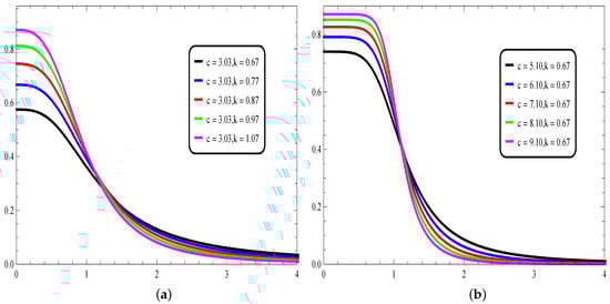
Figure 1. Plots showing the proposed pdf for different parameter values (a) fixing c and moving k, and (b) fixing k and moving c.

From this figure, various decreasing asymmetric shapes are observed, and the heavy right-tailed property is preserved. To the best of our knowledge, the proposed pdf is one of the rarest of its kind in the context of distance sampling.

On the other hand, since $g(0;c,k)=1$, we get

$$f(0;c,k)=\frac{c}{\beta \left(k-\frac{1}{c},\frac{1}{c}\right)}$$

and the population parameter D is given by

$$D=\frac{nf(0;c,k)}{2L}=\frac{nc}{2L\beta \left(k-\frac{1}{c},\frac{1}{c}\right)},$$

where L represents the total length of r lines $l_1,l_2,\dots ,l_r$, which are assumed to be non-overlapping and placed randomly in a specific region, and n represents the number of sighted objects collected based on the k lines. For the estimation of D, it is needed to estimate the parameter $f(0;c,k)$, which demonstrates that $f(0;c,k)$ plays a crucial role in this regard.

3. Some Statistical Properties

In this section, we determine some moment results that will help us estimate the parameter $f(0;c;k)$ and thus the population abundance. For any integer r, the rth moment of a random variable X with the pdf given in Equation (1) can be calculated as follows:

$${\mu }_r^{{}^{\prime }}=E\left(X^r\right)={\int }_0^{\infty }{x}^r\frac{c}{\beta \left(k-\frac{1}{c},\frac{1}{c}\right)}{\left(1+x^c\right)}^{-k}dx,$$

where E denotes the expectation operator. This moment exists in the mathematical sense if and only if $ck>r+1$. Under this condition and after some algebra, we can express it as a ratio of two beta functions as

$${\mu }_r^{{}^{\prime }}=\frac{1}{\beta \left(k-\frac{1}{c},\frac{1}{c}\right)}\beta \left(k-\frac{r+1}{c},\frac{r+1}{c}\right).$$

(2)

The mean and variance can be obtained from ${\mu }_1^{{}^{\prime }}$ and ${\mu }_2^{{}^{\prime }}$, provided that $ck>2$ and $ck>3$, respectively. They are calculated as follows:

$$\mu ={\mu }_1^{{}^{\prime }}=\frac{1}{c}f(0;c,k)\beta \left(k-\frac{2}{c},\frac{2}{c}\right)$$

(3)

and

$${\sigma }^2=\mathrm{Var}\left(X\right)=\frac{1}{c}f(0;c,k)\beta \left(k-\frac{3}{c},\frac{3}{c}\right)-{\left[\frac{1}{c}f(0;c,k)\beta \left(k-\frac{2}{c},\frac{2}{c}\right)\right]}^2.$$

The skewness and kurtosis of X can be determined based on Equation (2), provided that $ck>4$ and $ck>5$, respectively. They are defined as

$$\mathrm{Skewness}=\frac{{\mu }_3^{{}^{\prime }}-3{\mu }_2^{{}^{\prime }}\mu +2{\mu }^3}{{\sigma }^3},\mathrm{Kurtosis}=\frac{{\mu }_4^{{}^{\prime }}-4{\mu }_3^{{}^{\prime }}\mu +6{\mu }_2^{{}^{\prime }}{\mu }^2-3{\mu }^4}{{\sigma }^4},$$

according to Ghitany et al. [43] and Wackerly et al. [44], respectively. Table 1 displays various options for the model parameters c and k, as well as numerical values for the mean, variance, skewness, and kurtosis of X.

Table 1. Mean, variance, skewness and kurtosis for some parameter values.

Parameters		$\mathit{c}=2$
$\mathit{k}$	Mean	Variance	Skewness	Kurtosis
10	0.1906	0.0224	1.2042	20.5846
12	0.1720	0.0180	1.1630	20.8393
14	0.1579	0.0150	1.1354	21.0311
16	0.1468	0.0129	1.1156	21.1793
18	0.1378	0.0113	1.1007	21.2969
20	0.1302	0.0100	1.0891	21.3922
Parameters		$\mathit{k}=\mathbf{10}$
$\mathit{c}$	Mean	Variance	Skewness	Kurtosis
1	0.1250	0.0200	2.9397	23.3851
3	0.2429	0.0283	0.7322	29.2664
5	0.3099	0.0380	0.3675	40.6722
7	0.3497	0.0450	0.2222	46.3577
9	0.3759	0.0502	0.1489	49.4208
10	0.3858	0.0523	0.1252	50.4325

From this table, for the fixed value of c, the values of the skewness and kurtosis do not change much. However, the parameter k plays a crucial role in the asymmetric and flatness properties of the proposed pdf.

4. Inference

This section looks into statistical inferences about the parameter $f(0;c,k)$, assuming that c and k are unknown. We address the asymptotic distribution, the moments (M), and the maximum likelihood (ML) methods. In what follows, $x_1,x_2,\dots ,x_n$ represent the observed values of a random sample $X_1,X_2,\dots ,X_n$ drawn from the pdf $f(x;c,k)$ associated with the proposed detection function $g(x;c,k)$.

4.1. Moments Estimate of $f(0;c,k)$

Provided that $ck>2$, the model’s initial moment, as given in Equation (3), is

$$\mu =\frac{1}{c}f(0;c,k)\beta \left(k-\frac{2}{c},\frac{2}{c}\right),$$

which leads to estimate $f(0;c,k)$ under the following form:

$$\widehat{f}(0;c,k)=\frac{c\overline{x}}{\beta \left(k-\frac{2}{c},\frac{2}{c}\right)},$$

where $\overline{x}=(1/n){\sum }_{i=1}^n{x}_i$. Since c and k are supposed to be unknown, we have to use the moment estimates of c and k. For this purpose, assuming that $ck>r+1$, with $r=1$ and 2 in Equation (2), respectively, we have

$$\frac{1}{\beta \left(k-\frac{1}{c},\frac{1}{c}\right)}\beta \left(k-\frac{2}{c},\frac{2}{c}\right)=\overline{x}$$

(4)

and

$$\frac{1}{\beta \left(k-\frac{1}{c},\frac{1}{c}\right)}\beta \left(k-\frac{3}{c},\frac{3}{c}\right)=\frac{1}{n}\sum _{i=1}^n{x}_i^2.$$

(5)

Solving the equations above, one can find the moments estimates of c and k as ${\widehat{c}}_{mm}$ and ${\widehat{k}}_{mm}$, respectively. Hence, the moment estimate of $f(0;c,k)$ is ${\widehat{f}}_M\left(0\right)=f(0;{\widehat{c}}_{mm},{\widehat{k}}_{mm})$, with the following form:

$${\widehat{f}}_M\left(0\right)=\frac{{\widehat{c}}_{mm}\overline{x}}{\beta \left({\widehat{k}}_{mm}-\frac{2}{{\widehat{c}}_{mm}},\frac{2}{{\widehat{c}}_{mm}}\right)}.$$

4.2. Maximum Likelihood Estimate of $f(0;c,k)$

To obtain the ML estimate (MLE) of $f(0;c,k)$, we need to find the MLEs of c and k and proceed by the substitution approach. The likelihood function based on the pdf $f(x;c,k)$ is

$$\ell (c,k)=\sum _{i=1}^{n}log\left[f(x_i;c,k)\right]=nlogc-nlog\beta \left(k-\frac{1}{c},\frac{1}{c}\right)-k\sum _{i=1}^{n}log\left(1+x_i^c\right).$$

The MLEs of c and k, say $\widehat{c}$ and $\widehat{k}$, are determined by maximizing $\ell (c,k)$ with respect to c and k. They have no closed form, but can be calculated by utilizing a numerical method such as the Newton-Raphson method. Then, the MLE of $f(0;c,k)$ is ${\widehat{f}}_{ML}\left(0\right)=f(0;\widehat{c},\widehat{k})$.

Now, when $n\to \infty$, the random version of the vector ${(\widehat{c},\widehat{k})}^{\prime }$ is asymptotically ${\mathcal{N}}_2\left({(c,k)}^{\prime },\mathsf{\Sigma }\right)$, where $\mathsf{\Sigma }$ is the estimated variance–covariance matrix given by

$$\begin{array}{cc}\hfill \mathsf{\Sigma }& =-{\left.{\left(\begin{array}{cc}{U}_{cc}& U_{ck}\\ U_{kc}& U_{kk}\end{array}\right)}^{-1}\right|}_{c=\widehat{c},k=\widehat{k}},\hfill \end{array}$$

where $U_{cc}={\partial }^2\ell (c,k)/(\partial c^2)$, $U_{ck}={\partial }^2\ell (c,k)/(\partial c\partial k)$, $U_{kk}={\partial }^2\ell (c,k)/(\partial k^2)$, and $U_{kc}={\partial }^2\ell (c,k)/(\partial k\partial c)$. From this result and the Delta method, when $n\to \infty$, the random version of ${\widehat{f}}_{ML}\left(0\right)$ is asymptotically ${\mathcal{N}}_1\left(f(0;c,k),{\zeta }^2\right)$, where

$${\zeta }^2={\left[{\nabla }_{(c,k)}f(0;c,k)\right]}^{\prime }\mathsf{\Sigma }{\nabla }_{(c,k)}{f(0;c,k)|}_{c=\widehat{c},k=\widehat{k}}.$$

From this result and $\alpha \in (0,1)$, a $100(1-\alpha )\%$ confidence interval (CI) for $f(0;c,k)$ is given by

$$I_{f(0;c,k)}=\left[{\widehat{f}}_{ML}\left(0\right)\pm z_{\alpha /2}\zeta \right],$$

where $z_{\gamma }$ denotes the $100\gamma$th percentile of a standard normal distribution. Naturally, because $f(0;c,k)\ge 0$, the lower bound of the CI can be truncated to 0 if ${\widehat{f}}_{ML}\left(0\right)-z_{\alpha /2}\zeta \le 0$.

5. Simulation Study and Results

We now carry out a simulation study to examine the performance of the proposed model (PM) estimates, ${\widehat{f}}_M\left(0\right)$ and ${\widehat{f}}_{ML}\left(0\right)$, of $f(0;c,k)$ compared to some other existing estimates. The negative exponential model (NEM) estimate, ${\widehat{f}}_{1,ML}\left(0\right)$, the half normal model (HNM) estimate, ${\widehat{f}}_{2,ML}\left(0\right)$, and weighted exponential model (WEM) estimate, ${\widehat{f}}_{3,ML}\left(0\right)$ (see Saeed [45]), are considered in this regard.

To replicate the perpendicular distances, two alternative target detection functions are considered, as well as observations $x_1,x_2,\dots ,x_n$ of $X_1,X_2,\dots ,X_n$, with sample sizes of $n=50$, 100, 200, 300 and 500. These detection functions were chosen based on the requirement that they depict the many shapes that might appear in the specific field (see Eidous [22]). Target models for simulating perpendicular distances include:

• Exponential power (EP) detection function (see Pollock [5]):

  $$f\left(x\right)=\frac{e^{-x^{\beta }}}{\mathsf{\Gamma }\left(1+\frac{1}{\beta }\right)},x>0,\beta >1,$$

  (6)

  where $\mathsf{\Gamma }\left(x\right)={\int }_0^{\infty }{t}^{x-1}{e}^{-t}dt$ is the standard gamma function.
• Beta exponential (BE) detection function (see Eberhardt [9]):

  $$g\left(x\right)=(1+\beta ){\left(1-x\right)}^{\beta },0<x<1,\beta >0.$$

  (7)

To simulate the data, each model is truncated at some distances w. The truncated points of the EP and BE detection functions are $w=5$, 3, $2.5$ and 2, and $w=0.5$ and 1, respectively. For both models, several (arbitrary) values of $\beta$ are chosen. For each model, $n=50$, 100, 200, 300 and 500 sample sizes are considered with 1500 times the samples for the perpendicular distances that are randomly drawn.

Table 2 and Table 3 provide the relative biases (RBs) and the relative mean square errors (RMEs). We made the following observations based on these results.

Table 2. RBs and RMEs for the different estimates when the data are simulated from the EP model.

			Estimate
$\mathit{n}$	$\mathit{\beta }$	$\mathit{w}$	${\widehat{\mathit{f}}}_{\mathit{M}}\left(\mathbf{0}\right)$		${\widehat{\mathit{f}}}_{\mathit{ML}}\left(\mathbf{0}\right)$		${\widehat{\mathit{f}}}_{\mathbf{1},\mathit{ML}}\left(\mathbf{0}\right)$		${\widehat{\mathit{f}}}_{\mathbf{2},\mathit{ML}}\left(\mathbf{0}\right)$		${\widehat{\mathit{f}}}_{\mathbf{3},\mathit{ML}}\left(\mathbf{0}\right)$
			RB	RME	RB	RME	RB	RME	RB	RME	RB	RME
50	1	5	0.118	0.364	−0.165	0.150	0.052	0.151	0.385	0.394	0.182	0.213
100	1	5	0.080	0.342	−0.167	0.112	0.053	0.113	0.388	0.392	0.181	0.197
200	1	5	0.078	0.330	−0.169	0.062	0.043	0.080	0.394	0.396	0.189	0.196
300	1	5	0.062	0.327	−0.171	0.051	0.033	0.051	0.396	0.392	0.179	0.192
500	1	5	0.042	0.321	−0.175	0.032	0.023	0.045	0.394	0.393	0.167	0.186
50	1.5	3	−0.008	0.241	−0.133	0.139	0.402	0.435	0.133	0.164	0.090	0.157
100	1.5	3	−0.029	0.234	−0.137	0.138	0.397	0.414	0.135	0.151	0.087	0.125
200	1.5	3	−0.039	0.232	−0.139	0.136	0.389	0.398	0.142	0.150	0.081	0.104
300	1.5	3	−0.059	0.231	−0.141	0.134	0.386	0.391	0.132	0.142	0.080	0.100
500	1.5	3	−0.063	0.230	−0.148	0.131	0.381	0.390	0.121	0.140	0.075	0.024
50	2	2.5	−0.019	0.151	−0.100	0.104	0.601	0.625	0.023	0.109	0.245	0.279
100	2	2.5	−0.043	0.112	−0.102	0.063	0.593	0.608	0.017	0.078	0.239	0.260
200	2	2.5	−0.040	0.094	−0.110	0.040	0.575	0.581	0.005	0.050	0.225	0.234
300	2	2.5	−0.047	0.090	−0.115	0.021	0.542	0.556	0.002	0.040	0.220	0.212
500	2	2.5	−0.049	0.064	−0.119	0.014	0.535	0.520	0.001	0.020	0.212	0.210
50	2.5	2	−0.002	0.098	−0.064	0.074	0.704	0.724	0.116	0.152	0.325	0.351
100	2.5	2	−0.009	0.082	−0.068	0.073	0.697	0.708	0.108	0.129	0.320	0.334
200	2.5	2	−0.016	0.045	−0.069	0.071	0.696	0.702	0.106	0.118	0.319	0.327
300	2.5	2	−0.021	0.031	−0.074	0.068	0.692	0.700	0.102	0.112	0.315	0.321
500	2.5	2	−0.0625	0.015	−0.078	0.063	0.690	0.692	0.100	0.109	0.312	0.317

Table 3. RBs and RMEs for the different estimates when the data are simulated from the BE model.

			Estimate
$\mathit{n}$	$\mathit{\beta }$	$\mathit{w}$	${\widehat{\mathit{f}}}_{\mathit{M}}\left(\mathbf{0}\right)$		${\widehat{\mathit{f}}}_{\mathit{ML}}\left(\mathbf{0}\right)$		${\widehat{\mathit{f}}}_{\mathbf{1},\mathit{ML}}\left(\mathbf{0}\right)$		${\widehat{\mathit{f}}}_{\mathbf{2},\mathit{ML}}\left(\mathbf{0}\right)$		${\widehat{\mathit{f}}}_{\mathbf{3},\mathit{ML}}\left(\mathbf{0}\right)$
			RB	RME	RB	RME	RB	RME	RB	RME	RB	RME
50	1	0.5	0.085	0.099	0.070	0.091	0.509	0.555	0.191	0.223	0.284	0.256
100	1	0.5	0.076	0.081	0.062	0.073	0.488	0.518	0.189	0.204	0.243	0.222
200	1	0.5	0.044	0.062	0.044	0.047	0.401	0.511	0.172	0.190	0.201	0.201
300	1	0.5	0.032	0.038	0.028	0.035	0.396	0.500	0.153	0.184	0.192	0.195
500	1	0.5	0.017	0.029	0.009	0.027	0.351	0.482	0.148	0.167	0.191	0.194
50	1.5	1	0.101	0.128	0.172	0.189	0.411	0.485	0.179	0.202	0.168	0.200
100	1.5	1	0.092	0.113	0.143	0.157	0.432	0.417	0.157	0.189	0.146	0.186
200	1.5	1	0.080	0.106	0.111	0.120	0.323	0.351	0.138	0.155	0.117	0.170
300	1.5	1	0.063	0.101	0.106	0.118	0.321	0.334	0.129	0.142	0.106	0.162
500	1.5	1	0.041	0.093	0.100	0.112	0.317	0.311	0.113	0.139	0.101	0.157

• For all estimates, the values of the corresponding RMEs diminish as n grows. This strongly suggests that the various estimates are accurate estimates of $f(0;c,k)$.
• From Table 2 and Table 3, we also observe that ${\widehat{f}}_{ML}\left(0\right)$ provides smaller RBs and RMEs than those of ${\widehat{f}}_M\left(0\right)$, so we conclude that ${\widehat{f}}_{ML}\left(0\right)$ is better than ${\widehat{f}}_M\left(0\right)$.
• In addition, Table 2 and Table 3 show that the proposed estimates ${\widehat{f}}_{ML}\left(0\right)$ provide smaller RBs and RMEs than the NEM, HNM, and WEM estimates for all target detection functions considered. So, we can say that the proposed estimates are the best in comparison to those of the other competitors’ models.
• In Figure 2, Figure 3 and Figure 4, we plot the RMEs for ${\widehat{f}}_{ML}\left(0\right)$, ${\widehat{f}}_{1,ML}\left(0\right)$, ${\widehat{f}}_{2,ML}\left(0\right)$ and ${\widehat{f}}_{3,ML}\left(0\right)$, respectively. Based on these figures, we can say that our proposed estimates perform very well and they are acceptable for all the considered target detection functions.
  

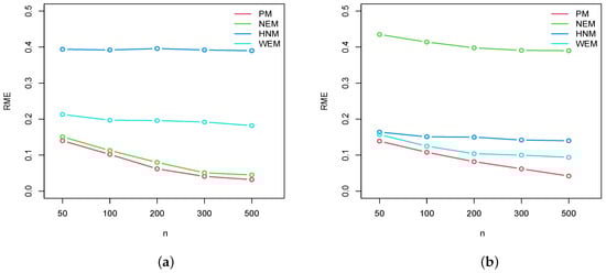  Figure 2. Plots of the RMEs for the EP model (a) $\beta =1$, $w=5$ and (b) $\beta =1.5$, $w=3$.
  

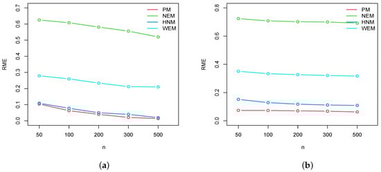  Figure 3. Plots of the RMEs for the EP model (a) $\beta =2$, $w=2.5$ and (b) $\beta =2.5$, $w=2$.
  

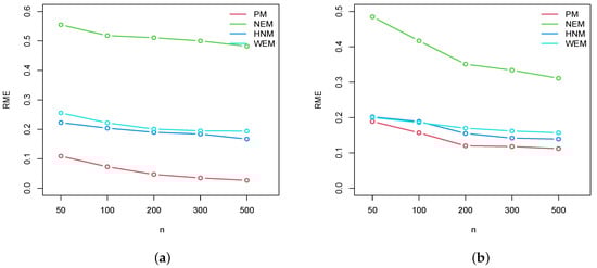  Figure 4. Plots of RME for the BE model (a) $\beta =1$, $w=0.5$ and (b) $\beta =1.5$, $w=1$.

As a result of the simulation, we can conclude that the proposed model fits the line transect data and that the proposed estimates of $f(0;c,k)$ and D are efficient. When compared to the NEM, HNM, and WEM, better results are obtained.

6. Real-World Data Application

The model selection and validation are the main topics of discussion in this section. A good model is carried out with the use of good judgment based on the information that is available. The chosen model must be adaptable enough to accurately represent the available data while taking into account the trade-off between the model’s complexity and ease of evaluation. Additionally, much effort must be directed to modeling behavior for both huge and small values of the relevant variable. In this context, validating the model is a step in the statistical process that includes a number of goodness-of-fit checks.

6.1. Competing Models

The performance of the proposed model is compared to a number of other existing models using goodness-of-fit evaluations. The following detection models are considered:

• Exponential quadratic model (EQM) (Burnham et al. [1]):

  $$g(x;c,k)=e^{-cx-k{x}^2},$$

  $$f(x;c,k)=\frac{2k{e}^{-cx-k{x}^2}}{e^{-c^2/4k}\sqrt{\pi }\mathrm{erfc}(c/2\sqrt{k})},x,c,k>0,$$

  where $\mathrm{erfc}\left(x\right)=(2/\sqrt{\pi }){\int }_0^x{e}^{-t^2}dt$ denotes the complementary error function.
• Weighted half-normal model (WHNM) (Eidous and Al-Eibood [23]):

  $$g(x;k)=(2-e^{-x^2/\left(2k\right)})e^{-x^2/\left(2k\right)},$$

  $$f(x;k)=\frac{2}{\sqrt{k}\sqrt{\pi }(2\sqrt{2}-1)}(2-e^{-x^2/\left(2k\right)})e^{-x^2/\left(2k\right)},x,k>0.$$
• Model (2015) (Eidous and Al-Eibood [22]):

  $$g(x;k)=4{\left(1-\frac{1}{2}{e}^{-kx/2}\right)}^2{e}^{-kx},$$

  $$f(x;k)=\frac{24k}{11}{\left(1-\frac{1}{2}{e}^{-kx/2}\right)}^2{e}^{-kx},x,k>0.$$
• Weighted exponential model (WEM) (Ababneh and Eidous [11]):

  $$g(x;k)=(2-e^{-kx})e^{-kx},$$

  $$f(x;k)=\frac{2k}{3}(2-e^{-kx})e^{-kx},x,k>0.$$
• Negative exponential model (NEM) (Gates et al. [2]):

  $$g(x;k)=e^{-kx},$$

  $$f(x;k)=k{e}^{-kx},x,k>0.$$

For comparison purposes and the data under consideration, we derive the MLEs from the relevant pdf of each detection model.

6.2. Perpendicular Distance Data Sets

Data set 1: Wooden stakes perpendicular distance data in meters.

The data set under consideration shows a number of perpendicular distances between wooden stakes in a sagebrush meadow east of Logan with a true density of $D=0.00375$ stake/meter. The data $x_1,x_2,\dots ,x_n$ are obtained by walking a single path of length $L=1000$ m, selecting a sample of objects ($n=67$ stakes) from a population of objects ($N=150$ stakes), and recording their associated perpendicular distances. The true value of $f\left(0\right)$ given n and D is thus 0.11029 (see (Karunamuni and Quinn [7]) and (Zhang [46])). Additionally, the size of the zone of interest (sagebrush meadow east) is $A=$ 40,000 m${}^2$, which was determined using the formula $D=N/A$, where $N=150$ (see Karunamuni and Quinn [7] and Zhang [46]).

The data are presented in Table 4. They have been reported and examined by Burnham et al. [1] and Barabesi [21]. With regard to the data set provided for wooden stakes, it can be seen that the perpendicular distance of 31.31 in Table 4 deviates substantially from the transect path as opposed to other ones. As a result, eliminating this extreme number will increase the estimation accuracy (see Zhang [46]). We thus remove the truncation point.

Table 4. Wooden stakes perpendicular distance data in meters.

2.02	0.45	10.40	3.61	0.92	1.00	3.40	2.90	8.16	6.47	5.66
2.95	3.96	0.09	11.82	14.23	2.44	1.61	6.50	8.27	4.85	1.47
18.60	0.41	0.40	0.20	11.59	3.17	7.10	10.71	3.86	6.05	6.42
3.79	15.24	3.47	3.05	7.93	18.15	10.05	4.41	1.27	13.72	6.25
3.59	9.04	7.68	4.89	9.10	3.25	8.49	6.08	0.40	9.33	0.53
1.23	1.67	4.53	3.12	3.05	6.60	4.40	4.97	3.17	7.67	18.16
4.08

Table 5 provides the essential statistics of the Wooden stakes data set.

Table 5. Wooden stakes data set descriptive summary.

n	Mean	Median	Standard Deviation	Skewness	Kurtosis	${\displaystyle \frac{\mathbf{Skewness}}{\mathbf{Kurtosis}}}$
67	5.7320	4.4124	4.5564	1.1083	3.8033	0.2914

Based on these results, it is clear that the data are skewed to the right, and our proposed model is suitable for this situation.

Data set 2: The Hemingway’s perpendicular distance data.

The second data set comes from Hemmingway’s research on several ungulates in Africa (see Burnham et al. [1]). They are presented in Table 6. The context is that 73 animals were discovered along a 60000-meter-long line transect. Using the sighting method, the perpendicular distances are calculated, with sighted angles and distances. The true density D and area A of the discovered items (which were not recorded during the survey) are not included in Hemmingway’s data set. However, the TRANSECT software, which adapts the estimates of $f\left(0\right)$ and D, which are, respectively, 0.0065 and 0.0396 animals per hectare (or 3.096106 animals per meter), creates the estimation technique.

Table 6. The Hemmingway’s data perpendicular distance data in meters.

0	0	0	0	0	0	0	0	8.72	10.5
22.3	26.0	26.0	30.5	30.5	31.7	34.2	35.1	38.0	41.0
42.1	50.8	55.1	58.5	63.6	64.3	65.0	68.8	71.1	71.8
71.9	72.1	73.1	76.6	77.6	78.1	84.0	84.5	86.0	86.0
87.0	90.0	92.3	94.0	96.4	96.4	106.0	115.0	123.0	123.0
129.0	129.0	143.0	143.0	150.0	151.0	153.0	157.0	161.0	164.0
164.0	164.0	166.0	175.0	188.0	193.0	200.0	200.0	246.0	260.0
272.0	378.0	400.0

The essential statistics of Hemmingway’s data are presented in Table 7.

Table 7. The Hemmingway’s data set descriptive summary.

n	Mean	Median	Standard Deviation	Skewness	Kurtosis	${\displaystyle \frac{\mathbf{Skewness}}{\mathbf{Kurtosis}}}$
73	99.2414	84.00	82.3732	1.36056	5.47687	0.248418

Table 8 and Table 9 present the MLEs of the parameter models, along with the associated standard errors (in parentheses), for Data sets 1 and 2, respectively.

Table 8. MLEs and their standard errors for Data set 1.

Model	c	k
PM	1.7160	1.1112
	(0.1251)	(0.5277)
EQM	0.0369	0.0073
	(0.0132)	(0.0027)
WHNM	-	42.6802
	-	(4.1761)
Model (2015)	-	0.2369
	-	(0.1521)
WEM	-	0.2042
	-	(0.1210)
NEM	-	0.1744
	-	(0.1210)

Table 9. MLEs and their standard errors for Data set 2.

Model	c	k
PM	1.2001	1.0330
	(0.5121)	(0.6129)
EQM	0.0040	0.0011
	(0.0031)	(0.0007)
WHNM	-	6.9237
	-	(3.4127)
Model (2015)	-	0.0135
	-	(0.0121)
WEM	-	0.0117
	-	(0.1012)
NEM	-	0.0100
	-	(0.0174)

From these tables, it is worth noting that the condition $ck>1$ and $c>1$ are satisfied with the parameter estimates, and that the standard errors are quite moderate for all the models.

In order to compare the fit performance of the considered models for the analysis of Data sets 1 and 2, the following standard criteria are used: Akaike information criterion (AIC), corrected AIC (CAIC), Bayesian information criterion (BIC), and Hannan–Quinn information criterion (HQIC). Table 10 and Table 11 display their values. We see that our model has the lowest values of these information criteria. As a result, we can draw the conclusion that the proposed model is the best in this setting.

Table 10. Information criteria for Data set 1.

Detection Models	AIC	CAIC	BIC	HQIC
PM	349.613	349.801	354.023	351.358
EQM	367.311	367.499	371.720	369.056
WHNM	367.503	367.591	371.813	369.058
Model (2015)	366.330	366.392	368.535	366.392
WEM	367.052	367.113	369.256	367.924
NEM	369.723	369.785	371.928	370.596

Table 11. Information criteria for Data set 2.

Detection Models	AIC	CAIC	BIC	HQIC
PM	812.461	815.431	810.112	817.012
EQM	817.397	817.454	819.688	818.310
WHNM	817.059	817.116	819.35	817.972
Model (2015)	816.553	816.609	818.843	817.466
WEM	817.397	817.454	819.688	818.310
NEM	819.243	819.299	821.533	820.156

With Data sets 1 and 2 and the proposed model, the CIs of the pdf at 0 based on the MLEs are determined in Table 12 (with appropriate truncation for the lower bound of the intervals).

Table 12. Confidence intervals for Data sets 1 and 2, respectively.

CI	c	k	$\mathit{f}\left(0\right)$
$95\%$	[0.626, 2.810]	[0.022, 2.200]	[0, 1.723]
$99\%$	[0.286, 3.15]	[0, 2.547]	[0, 2.06]
CI	$\mathit{c}$	$\mathit{k}$	$\mathit{f}\left(\mathbf{0}\right)$
$95\%$	[0, 2.08]	[0, 2.48]	[0, 2.03]
$99\%$	[0, 2.68]	[0, 3.08]	[0, 2.63]

The estimated population abundances $\widehat{D}$ and ${\widehat{f}}_{ML}\left(0\right)$ are calculated using the MLEs of all the examined models. The theoretical standard deviation of the model is denoted by $SD$ and the sample standard deviation is $\widehat{SD}$. The values of ${\widehat{f}}_{ML}\left(0\right)$ and $|\widehat{SD}-SD|$ are collected in Table 13 and Table 14 for Data sets 1 and 2, respectively. In these tables, the proposed model has the lowest $|\widehat{SD}-SD|$. Furthermore, among the tested detection models, it is the most similar to the actual $f\left(0\right)$ and D.

Table 13. Estimated $f\left(0\right)$ and population abundance D for Data set 1 using $|\widehat{SD}-SD|$.

Detection Models	${\widehat{\mathit{f}}}_{\mathit{ML}}\left(0\right)$	$\widehat{\mathit{D}}$	$|\widehat{\mathit{SD}}-\mathit{SD}|$
PM	0.1101	0.0031	0.1977
EQM	0.1220	0.0040	1.0341
WHNM	0.0940	0.0032	0.3396
Model (2015)	0.1291	0.0043	0.4167
WEM	0.1360	0.0045	0.6691
NEM	0.1740	0.0058	1.1765

Table 14. Estimated $f\left(0\right)$ and population abundance D for Data set 2 using $|\widehat{SD}-SD|$.

Detection Models	${\widehat{\mathit{f}}}_{\mathit{ML}}\left(0\right)$	$\widehat{\mathit{D}}$	$|\widehat{\mathit{SD}}-\mathit{SD}|$
PM	0.0064	0.0345	0.1896
EQM	0.0078	0.0002	0.2341
WHNM	0.0062	0.0002	0.3396
Model (2015)	0.0074	0.0002	0.3170
WEM	0.0078	0.0002	0.5219
NEM	0.0100	0.0003	1.2180

7. Conclusions

This work introduced and examined a novel detection model based on the survival function of the Burr XII distribution. Through an in-depth investigation, it revealed itself to be excellent for line transect data. One of its qualities is that it is adaptable to some kinds of line-transect data because it has a heavy right tail with modulating skewness (or asymmetry) and kurtosis thanks to two parameters. For the raw moments, closed-form expressions were established. Statistical techniques are employed to estimate these parameters. They are the moments and maximum likelihood techniques. The resulting estimates do not exist in a closed form but can be computed with the help of software. According to our simulation results, they are efficient for estimating population abundance. Moreover, the performance of our model compared favorably to other models for important data sets. We thus recommend the use of our new “Burr XII detection model” in similar statistical scenarios. A possible extension is to investigate the addition of a scale parameter in the detection function; however, additional work must be carried out on the definition of the normalization constant, and the proposed methodology must be adapted. We leave this perspective for future work.

References

- Burnham, K.P.; Anderson, D.R.; Laake, J.L. Estimation of density from line transect sampling of biological populations. Wildl. Monogr. 1980, 72, 3–202. [Google Scholar]
- Gates, C.E.; Marshall, W.H.; Olson, D.P. Line transect method of estimating grouse population densities. Biometrics 1968, 24, 135–145. [Google Scholar] [CrossRef] [PubMed]
- Hemingway, P. Field trials of the line transect method of sampling large populations of herbivores. In The Scientific Management of Animal and Plant Communities for Conservation; Blackwell: Oxford, UK, 1971; pp. 405–411. [Google Scholar]
- Burnham, K.P.; Anderson, D.R. Mathematical models for nonparametric inferences from line transect data. Biometrics 1976, 32, 325–336. [Google Scholar] [CrossRef] [PubMed]
- Pollock, K.H. A family of density estimators for line-transect sampling. Biometrics 1978, 34, 475–478. [Google Scholar] [CrossRef]
- Ramsey, F.L. Parametric models for line transect surveys. Biometrika 1979, 66, 505–512. [Google Scholar] [CrossRef]
- Karunamuni, R.J.; Quinn, T.J. Bayesian estimation of animal abundance for line transect sampling. Biometrics 1995, 51, 1325–1337. [Google Scholar] [CrossRef]
- Buckland, S.T. Perpendicular distance models for line transect sampling. Biometrics 1985, 41, 177–195. [Google Scholar] [CrossRef]
- Eberhardt, L.L. Transect methods for population studies. J. Wildl. Manag. 1978, 42, 1–31. [Google Scholar] [CrossRef]
- Eidous, U. A parametric family for density estimation in line transect sampling. Basic Sci. Eng. 2004, 13, 315–326. [Google Scholar]
- Ababneh, F.; Eidous, O.M. A weighted exponential detection function model for line transect data. J. Mod. Appl. Stat. Methods 2012, 11, 11. [Google Scholar] [CrossRef]
- Quinn, T.J.; Gallucci, V.F. Parametric Models for Line-Transect Estimators of Abundance. Ecology 1980, 61, 293–302. [Google Scholar] [CrossRef]
- Eidous, O.; Al-Eibood, F. A bias-corrected histogram estimator for line transect sampling. Commun.-Stat.-Theory Methods 2018, 47, 3675–3686. [Google Scholar] [CrossRef]
- Buckland, S.T.; Turnock, B.J. A robust line transect method. Biometrics 1992, 48, 901–909. [Google Scholar] [CrossRef]
- Amstrup, S.C.; Durner, G.M.; McDonald, T.L.; Mulcahy, D.M.; Garner, G.W. Comparing movement patterns of satellite-tagged male and female polar bears. Can. J. Zool. 2001, 79, 2147–2158. [Google Scholar] [CrossRef]
- Alpizar-Jara, R.; Pollock, K.H. A combination line transect and capture-recapture sampling model for multiple observers in aerial surveys. Environ. Ecol. Stat. 1996, 3, 311–327. [Google Scholar] [CrossRef]
- Becker, E.F.; Quang, P.X. A gamma-shaped detection function for line-transect surveys with mark-recapture and covariate data. J. Agric. Biol. Environ. Stat. 2009, 14, 207–223. [Google Scholar] [CrossRef]
- Horvitz, D.G.; Thompson, D.J. A generalization of sampling without replacement from a finite universe. J. Am. Stat. Assoc. 1952, 47, 663–685. [Google Scholar] [CrossRef]
- Borchers, D.L.; Buckland, S.T.; Goedhart, P.W.; Clarke, E.D.; Hedley, S.L. Horvitz-Thompson estimators for double-platform line transect surveys. Biometrics 1998, 54, 1221–1237. [Google Scholar] [CrossRef]
- Marques, F.F.; Buckland, S.T.; Goffin, D.; Dixon, C.E.; Borchers, D.L.; Mayle, B.A.; Peace, A.J. Estimating deer abundance from line transect surveys of dung: Sika deer in southern Scotland. J. Appl. Ecol. 2001, 38, 349–363. [Google Scholar] [CrossRef]
- Barabesi, L. Local likelihood density estimation in line transect sampling. Environ. Off. J. Int. Environ. Soc. 2000, 11, 413–422. [Google Scholar] [CrossRef]
- Eidous, O.M. Nonparametric Estimation of f(0) Applying Line Transect Data with and without the Shoulder Condition. J. Inf. Optim. Sci. 2015, 36, 301–315. [Google Scholar] [CrossRef]
- Eidous, O.; Al-Salman, S. One-term approximation for normal distribution function. Math. Stat. 2016, 4, 15–18. [Google Scholar] [CrossRef]
- Jang, W.; Loh, J.M. Density estimation for grouped data with application to line transect sampling. Ann. Appl. Stat. 2010, 4, 893–915. [Google Scholar] [CrossRef]
- Seber, G.A.F. The Estimation of Animal Abundance and Related Parameters; Macmillan Publishing Company: New York, NY, USA, 1982. [Google Scholar]
- Strindberg, S.; Buckland, S.T. Zigzag survey designs in line transect sampling. J. Agric. Biol. Environ. Stat. 2004, 9, 443–461. [Google Scholar] [CrossRef]
- Quang, P.X.; Becker, E.F. Combining line transect and double count sampling techniques for aerial surveys. J. Agricult. Biol. Environ. Stat. 1997, 2, 230–242. [Google Scholar] [CrossRef]
- Drummer, T.D.; McDonald, L.L. Size bias in line transect sampling. Biometrics 1987, 43, 13–21. [Google Scholar] [CrossRef]
- Burnham, K.P.; Anderson, D.R. The need for distance data in transect counts. J. Wildl. Manag. 1984, 48, 1248–1254. [Google Scholar] [CrossRef]
- Routledge, R.D.; Fyfe, D.A. Confidence limits for line transect estimates based on shape restrictions. J. Wildl. Manag. 1992, 57, 402–407. [Google Scholar] [CrossRef]
- Southwell, C. Evaluation of walked line transect counts for estimating macropod density. J. Wildl. Manag. 1994, 58, 348–356. [Google Scholar] [CrossRef]
- Southwell, C.; Paxton, C.G.; Borchers, D.; Boveng, P.; Rogers, T.; William, K. Uncommon or cryptic? Challenges in estimating leopard seal abundance by conventional but state-of-the-art methods. Deep. Sea Res. Part I Oceanogr. Res. Pap. 2008, 55, 519–531. [Google Scholar] [CrossRef]
- Brockelman, W.Y.; Srikosamatara, S. Estimation of density of gibbon groups by use of loud songs. Am. J. Primatol. 1993, 29, 93–108. [Google Scholar] [CrossRef] [PubMed]
- Chen, S.X. A kernel estimate for the density of a biological population by using line transect sampling. J. R. Stat. Soc. Ser. Appl. Stat. 1996, 45, 135–150. [Google Scholar] [CrossRef]
- Melville, G.J.; Welsh, A.H. Line transect sampling in small regions. Biometrics 2001, 57, 1130–1137. [Google Scholar] [CrossRef] [PubMed]
- Ely, R.J.; Thomas, D.A. Cultural diversity at work: The effects of diversity perspectives on work group processes and outcomes. Adm. Sci. Q. 2001, 46, 229–273. [Google Scholar] [CrossRef]
- Porteus, T.A.; Richardson, S.M.; Reynolds, J.C. The importance of survey design in distance sampling: Field evaluation using domestic sheep. Wildl. Res. 2011, 38, 221–234. [Google Scholar] [CrossRef]
- Laake, J.; Dawson, M.J.; Hone, J. Visibility bias in aerial survey: Mark–recapture, line-transect or both? Wildl. Res. 2008, 35, 299–309. [Google Scholar] [CrossRef]
- Schmidt, J.H.; Rattenbury, K.L.; Lawler, J.P.; Maccluskie, M.C. Using distance sampling and hierarchical models to improve estimates of Dall’s sheep abundance. J. Wildl. Manag. 2012, 76, 317–327. [Google Scholar] [CrossRef]
- Fewster, R.M.; Southwell, C.; Borchers, D.L.; Buckland, S.T.; Pople, A.R. The influence of animal mobility on the assumption of uniform distances in aerial line-transect surveys. Wildl. Res. 2008, 35, 275–288. [Google Scholar] [CrossRef]
- Rodriguez, R.N. A guide to the Burr type XII distributions. Biometrika 1977, 64, 129–134. [Google Scholar] [CrossRef]
- Al-Hussaini, E.K. A characterization of the Burr type XII distribution. Appl. Math. Lett. 1991, 4, 59–61. [Google Scholar] [CrossRef]
- Ghitany, M.E.; Al-Mutairi, D.K.; Balakrishnan, N.; Al-Enezi, L.J. Power Lindley distribution and associated inference. Computational Stat. Data Anal. 2013, 64, 20–33. [Google Scholar] [CrossRef]
- Wackerly, D.; Mendenhall, W.; Scheaffer, R.L. Mathematical Statistics with Applications; Cengage Learning: Belmont, CA, USA, 2014. [Google Scholar]
- Saeed, G.A.A. New Parametric Model for Grouped and Ungrouped Line Transect Data. Ph.D. Thesis, Yarmouk University, Irbid, Jordan, 2013. [Google Scholar]
- Zhang, S. Generalized likelihood ratio test for the shoulder condition in line transect sampling. Commun. Stat.-Theory Methods 2001, 30, 2343–2354. [Google Scholar] [CrossRef]
Disclaimer/Publisher’s Note: The statements, opinions and data contained in all publications are solely those of the individual author(s) and contributor(s) and not of MDPI and/or the editor(s). MDPI and/or the editor(s) disclaim responsibility for any injury to people or property resulting from any ideas, methods, instructions or products referred to in the content. |
© 2023 by the authors. Licensee MDPI, Basel, Switzerland. This article is an open access article distributed under the terms and conditions of the Creative Commons Attribution (CC BY) license (https://creativecommons.org/licenses/by/4.0/).