Chaos Control of a Delayed Tri-Trophic Food Chain Model with Fear and Its Carry Over Effects

Abstract

One of the main objectives of theoretical ecologists involves finding mechanisms to control the chaos in ecological models to maintain positive densities of the species. Numerous researchers have suggested that, apart from the direct killing in the prey–predator relationship, there are some indirect effects, such as fear of predation. Induced fear can lead to slowing down the growth rate of the prey species, and this non-chemical strategy can be carried over to successive seasons or upcoming generations. In this work, we explore the impact of fear due to predation and its carry-over effect (COE) in a delayed tri-trophic food chain model, whereas the Holling type-II functional response is used to determine the interference among the species. The proposed model is an asymmetric interaction food chain model since the species in this model only kills other species. The growth rate of prey and middle predators is affected due to the respective fear of predation by middle and special predators. The non-delayed model considered in this paper generalizes the models developed by Hastings–Powell and Panday et al. The gestation delay in the special predator’s growth term is incorporated into the proposed model. We determined the essential conditions for the existence of ecologically feasible equilibrium points and their local and global stability. Furthermore, we developed the conditions for the occurrence of the Hopf bifurcation around an interior equilibrium to seek periodic behaviors of delayed and non-delayed models. Numerical examples were performed to justify the proposed theoretical findings and to show the impacts of fear and its COE parameters on the system dynamics through phase portraits, the time series of solutions, and bifurcation diagrams. We discovered that the chaotic behavior of the food chain model can be controlled by using the fear effect and its COE parameters. The dynamics of the delayed food chain model with the fear effect and its COEs are further explored in our findings. Our theoretical findings clearly provide a mechanism to protect and control species populations in ecological systems. It is also essential for developing optimized harvesting strategies in fisheries and pest management in agriculture.

1. Introduction

Theoretical ecologists are focusing on the study of interactions between living organisms and their environments; this is because the study is important in the formation of an ecosystem. In the 1920s, Lotka and Volterra individually developed first-order ordinary differential equations to report on the interactions between two species. Since then, researchers have been interested in modeling and analyzing interactions between species; see [1,2] and references therein. Different types of mathematical models, including ordinary [2], partial [3], non-integer order [4], and difference equation [5,6], have been developed in order to make use of different environmental factors in predator–prey models, such as Allee effects, prey refuges, stage structure, harvesting, toxic effects, and environmental fluctuations. On the other hand, the existence of chaos in dynamical systems is quite obvious due to the presence of nonlinear terms. Predicting the future evolution of chaotic systems remains a difficult task due to its sensitivity to the initial condition and system parameters. In order to narrow this gap, the problem of chaos control has become a hot topic among researchers in various fields, such as biomedical systems [7], ecological models [8], convection models [9], etc. The chaos control approach leads a chaotic system to a limit cycle or an asymptotically stable state. In contrast, the problem of chaotification is becoming more popular because of its applications in the fields of secure communication, encryption, description, signal processing, etc., where chaotic behavior is a desired phenomenon; see [10,11,12] for more details. In ecological systems, chaotic phenomena need to be controlled in order to predict how species will evolve in the future. The chaotic behaviors in the three-species food chain were initially noticed by Hastings and Powell [13]. Since then, many academics have attempted to address the issue of how to use ecological factors to regulate chaos in food chain models (see [14,15,16,17,18,19,20]). The authors of [15] demonstrated that the food chain model exhibited chaos due to the parameters of prey growth rate and predator interference. Nath et al. [17] showed that chaos can be controlled through prey refuge and the Allee effect in a food chain model. To regulate the system, the intermediate predator harvesting strategy was introduced in reference [18]. The chaotic behavior of the prey–predator–parasite model can be controlled through a prey-harvesting strategy [19]. Recently, Nitu and Vikas [20] considered the tri-trophic food model, where the cannibalism effect was applied to middle predators to control the system dynamics.

From a biological perspective, interspecific killing among carnivores is a much more frequent issue. The interaction among species is symmetrical if both species kill each other, and the interaction is asymmetrical if one species kills another [21]. On the other hand, the relationship between predator and prey is impacted not only by the method of direct encounters but also by an indirect effect (such as fear), which also alters the prey’s usual characteristics [22,23]. The altered characteristics could be associated with the prey’s nature, morphology, and habitat. To escape from the predation risk, the prey always attempts to change its usual habitat to a safer location [24]. As a consequence, the short-term survivability of the prey is increasing; it has started to decrease in the long term. Numerous theoretical and experimental studies indicate that indirect effects can have notable impacts on the dynamics of predator–prey interactions [25,26,27,28,29,30,31,32,33]. The growth rate of elk in the Greater Yellowstone Ecosystem is affected by their fear of wolves [25], while mule deer shorten their feeding activity due to the risk of mountain lion predation. The authors of [22] discovered that predator fear of song sparrows resulted in a 40% reduction in the number of offspring produced, even in the absence of direct contact with predators. Suraci et al. [27] experimented for over a month on mesocarnivores (raccoons) by creating fear through the sounds of their predators and found that the fear of large carnivores reduced the raccoon’s foraging behavior by 66% and increased awareness. Based on the aforementioned ideas, Wang et al. [23] mathematically modeled the impact of fear on the growth of the prey and observed that the cost of fear had a considerable impact on the dynamics of predator–prey interactions. Moreover, they noticed that fear can have a stabilizing effect on system dynamics. Panday et al. [31] examined the dynamics of a food chain model with predation fear and they concluded that suitable fear effects can regularize the system from chaotic oscillation to stable. They also noticed that the top predator can lead to an extinction stage if the cost of fear of intermediate predators goes up. In [29], Sasmal et al. dealt with the dynamics of the food chain model with the fear effect and group defense strategy among prey. In [34], Mishra et al. studied the effect of fear in the agroecosystem. By utilizing the B-D functional response, Debnath et al. [35] investigated the dynamics of a food chain model, and found that fear effects as well as mutual interference parameters among species can control the system dynamics.

The term “COE” often emerges from repetitive measures in clinical investigations. It has been recently applied to ecological and evolutionary concerns and applies to a wide range of circumstances. From an ecological point of view, COEs measure an individual species’ past learning, and can influence the current performance [36]. The COE has a positive influence on the species community when past habitation is lost because some fatal or non-fatal effects are of poor quality, and it has a negative influence when the lost habitation is of high quality [37]. COEs can occur over several seasons or even one season (i.e., changes in physiological behavior within a season). Experiments conducted in previous works [38,39,40] show that amphibians, fish, marine insects, marine invertebrates, and other animals can experience carry-over effects in short periods of time and within a single season. Thus, emerging perspectives among ecologists show the importance of COEs in mathematical modeling; see [37,41,42,43]. Sasmal and Takeuchi [42] incorporated predation fear and its COEs into models of prey–predator interactions and showed that fear and COE parameters can have significant impacts on system stability. Dubey and Sasmal [43] considered a phytoplankton–zooplankton fish system, where zooplankton growth rates are influenced by fish-induced fear and the COEs. In addition, they pointed out that the system exhibited chaotic behavior for medium values of COE parameters, and the system became stable or periodic dynamics occurred for lower and higher values. Thus, incorporating COEs into an ecological model showed more insight into the factors that affected the species in the ecosystem.

Time delays in ecology are unavoidable because of some lags observed in ecological processes, such as maturation time, gestation, and handling time. Such time lags in ecological systems may produce more complex system dynamics. Thus, studying the dynamical features of ecological models with time lags has become an important topic among theoretical ecologists in the last decade, (see [32,44,45,46,47,48,49] and references therein). To explore the dynamics of a food chain model, Pal et al. [45] and Upadhyay et al. [46], respectively, have taken the gestation delays of top predators only and both predators into account; they pointed out that delays significantly affected system stability. Recently, two different delays were established and analyzed in a tri-trophic food chain model by Surosh et al. in reference [48]. To construct a more appropriate ecological model, it is important to include time lag in it.

Population ecologists are usually interested in forecasting the future population density of a species in an ecological system to maintain a healthy ecosystem. Most ecological systems are nonlinear, resulting in chaotic behaviors that need to be controlled in order to predict how the ecological systems will evolve in the future. In this connection, researchers have attempted to control chaos in ecological systems through various control methods. Controlling chaotic behavior in an ecological system must involve methods that are easy to use and have no negative influence on the real ecosystem. The artificial induction of fear among prey species by utilizing the sounds or vocal cues of the appropriate predators in real ecological systems is a control strategy that is crucial in preventing the extinction stage of interacting species. This fear lets the prey know to stay away from the predator and protects the prey species, as well as causes changes in its own characteristics. However, the prey learns about the fear induced and carries this information into future generations or upcoming generations, which makes it act again with its usual characteristics. As a result, induced fear among prey species fails to control the system’s chaotic dynamics. To overcome this situation, a non-chemical method, the concept of fear and fear-induced COE, is incorporated into ecological models. Moreover, there is still enough room to explore the dynamics of ecological models by introducing various ecological factors. To the best of our knowledge, there has been no work devoted to the three-species food chain model with fear-induced COEs in the growth terms of both prey and middle predators. This prompted our current investigation.

Inspired by the ideas of a fear-induced COE given in reference [42,43], we considered the chaos control of a tri-trophic food chain model in which the growth terms of prey and the middle predator were influenced by a fear-induced COE due to the predation risk. The relationships between the species followed the Holling type-II functional response. The developed model is an asymmetric food chain model since middle predators kill only prey and special predators kill only middle predators. To control the chaotic dynamics of the proposed system, a novel non-chemical method was imposed through varying fear and fear-induced COE parameters. The proposed method is based on the idea that vocal cues or sounds can be used to induce fear and that this process is carried over by prey species to the upcoming season or generation. Furthermore, we consider gestation delay in the growth terms of special predators. We derived local and global stability criteria and the Hopf bifurcation analysis of the integrated model. In addition, we incorporated gestation delay into the proposed and analyzed the local stability and bifurcation of the delayed model. The numerical results demonstrate the effectiveness of the novel method and confirm the theoretical results. The main contributions of this paper are as follows:

i.

We propose a chaos control strategy based on inducing fear and its COEs in the prey and middle predator growth terms.

ii.

We analyze how induced fear and its COE parameters affect the population densities of the species involved in the proposed model.

iii.

Fear-induced COEs in the growth terms of both prey and middle predators are taken into account in this paper. This approach is different from other works in the literature.

iv.

We determine the impact of the gestation delay of a special predator on the dynamics of the system.

The model considered in this paper generalizes the models investigated in reference [13,31,45]. If the prey can learn about artificial vocal cues, then our theoretical findings clearly provide mechanisms to protect species in ecological systems. Moreover, the model suggested in this paper works better in places where there are three levels of food chains. It is also essential for developing optimized harvesting strategies in fisheries and pest management in agriculture.

The structure of the article is as follows. We provide a three-species food chain model with fear and its COEs in Section 2. Section 3 derives the preliminaries of a nonlinear food chain model. The chaos control of the tri-trophic food chain model is covered in Section 4. In Section 5, the food chain model is modified and examined with time delay. Selected numerical results are presented in Section 6 to support our proposed theoretical findings. Finally, in Section 7, we present the conclusions of the proposed study and suggest future research.

2. Description of the Tri-Trophic Food Chain Model

Mathematical models that describe the dynamics of a population can be categorized according to a continuous-time domain or a discrete-time domain. A continuous-time model is typically more appropriate if the species involved in the system have generations that overlap and births that are spaced throughout the year. Hastings–Powell [13] initially discovered chaos control in a continuous food chain model, and since then, several authors have attempted to control chaos by introducing new strategies [16,31,35]. In general, tritrophic food chains consist of prey, middle, and special predators at the bottom, middle, and top trophic levels. Hastings–Powell [13] developed a food chain model in the form:

$$\begin{array}{c}\hfill \begin{array}{c}{\displaystyle \frac{dU\left(T\right)}{dT}=R_{0}U\left(T\right)\left({\displaystyle 1-\frac{U\left(T\right)}{K}}\right)-\frac{C_1{A}_{1}U\left(T\right)V\left(T\right)}{B_1+U\left(T\right)},}\hfill \\ {\displaystyle \frac{dV\left(T\right)}{dT}=\frac{A_{1}U\left(T\right)V\left(T\right)}{B_1+U\left(T\right)}-D_{1}V\left(T\right)-\frac{A_{2}V\left(T\right)W\left(T\right)}{B_2+V\left(T\right)},}\hfill \\ {\displaystyle \frac{dW\left(T\right)}{dT}=\frac{C_2{A}_{2}V\left(T\right)W\left(T\right)}{B_2+V\left(T\right)}-D_{2}W\left(T\right),}\hfill \end{array}\end{array}$$

(1)

where $U\left(T\right),V\left(T\right)$, and $W\left(T\right)$ are the respective densities of prey, middle, and special predators at time T. The system parameters are all considered to be positive [13]. $R_0$ and K are the growth rates of the prey and environmental support capacity. $A_1$ (or $A_2$) is the maximum attack rate of the middle (or special) predator. $B_1$ (or $B_2$) represents the half-saturation coefficient of the prey (or middle predator). $C_1^{-1}$ (or $C_2$) indicates the conversion efficiencies of the middle (or special) predator. $D_1$ (or $D_2$) is the death rate of the middle (or special) predator. To simplify the notation, the state variables $U\left(T\right),V\left(T\right),$ and $W\left(T\right)$ are denoted by $U,V,$ and $W,$ respectively. By introducing the effect of fear in model (1), Panday et al. [31] extended the model given (1) into the following form

$$\begin{array}{c}\hfill \begin{array}{c}{\displaystyle \frac{dU}{dT}=R_{0}U\left({\displaystyle 1-\frac{U}{K}}\right)·\frac{1}{1+F_{1}V}-\frac{C_1{A}_{1}UV}{B_1+U},}\hfill \\ {\displaystyle \frac{dV}{dT}=\frac{A_{1}UV}{B_1+U}·\frac{1}{1+F_{2}W}-D_{1}V-\frac{A_{2}VW}{B_2+V},}\hfill \\ {\displaystyle \frac{dW}{dT}=\frac{C_2{A}_{2}VW}{B_2+V}-D_{2}W,}\hfill \end{array}\end{array}$$

(2)

where $F_1$ and $F_2$ represent the intensity of fear in the prey and middle predator population, respectively. However, the prey carries over some information from previous predation attacks to subsequent generations. The carry-over information affects the growth rate of the species [42,43]. Taking into account the above viewpoints, we extend model (2) by introducing fear-induced COEs. Then the system is given as follows:

$$\begin{array}{c}\hfill \begin{array}{c}{\displaystyle \frac{dU}{dT}=R_{0}U\left({\displaystyle 1-\frac{U}{K}}\right)·\frac{1+E_{1}U}{1+E_{1}U+F_{1}V}-\frac{C_1{A}_{1}UV}{B_1+U},}\hfill \\ {\displaystyle \frac{dV}{dT}=\frac{A_{1}UV}{B_1+U}·\frac{1+E_{2}V}{1+E_{2}V+F_{2}W}-D_{1}V-\frac{A_{2}VW}{B_2+V},}\hfill \\ {\displaystyle \frac{dW}{dT}=\frac{C_2{A}_{2}VW}{B_2+V}-D_{2}W,}\hfill \end{array}\end{array}$$

(3)

where $E_1$ and $E_2$ are the carry-over effect parameters due to the fear $F_1$ and $F_2$, respectively. In model (3), we introduce the functions $\Phi (E_1,F_1,U,V)=\frac{1 + E_{1}U}{1 + E_{1}U + F_{1}V}$ and $\Psi (E_2,F_2,V,W)=\frac{1 + E_{2}V}{1 + E_{2}V + F_{2}W}$, which represent fear and its COE in the interaction between the species. The functions $\Phi$ and $\Psi$ satisfy the following characteristics associated with fear and its COE [42]:

• $\Phi (E_1,0,U,V)=1$ and $\Psi (E_2,0,V,W)=1,$
• $\Phi (E_1,F_1,U,0)=1$ and $\Psi (E_2,F_2,V,0)=1,$
• ${lim}_{F_1\to \infty }\Phi =0$ and ${lim}_{F_2\to \infty }\Psi =0,$
• ${lim}_{V\to \infty }\Phi =0$ and ${lim}_{W\to \infty }\Psi =0,$
• $\frac{\partial \Phi }{\partial F_1}<0,\frac{\partial \Phi }{\partial V}<0$ and $\frac{\partial \Psi }{\partial F_2}<0,\frac{\partial \Psi }{\partial W}<0.$

Further, $\Phi$ and $\Psi$ satisfy the following characteristics associated with COE:

• $\frac{\partial \Phi }{\partial E_1}=\frac{F_{1}UV}{{(1 + E_{1}U + F_{1}V)}^2}>0$ and $\frac{\partial \Psi }{\partial E_2}=\frac{F_{2}VW}{{(1 + E_{2}V + F_{2}W)}^2}>0$, which indicates the positive effects of COE as a result of lessons learned from earlier seasons or experiences.
• $\frac{\partial \Phi }{\partial U}=\frac{F_1{E}_{1}V}{{(1 + E_{1}U + F_{1}V)}^2}>0$ and $\frac{\partial \Psi }{\partial V}=\frac{F_2{E}_{2}W}{{(1 + E_{2}V + F_{2}W)}^2}>0$, as the population densities of the prey and middle predator increase, respectively, increasing their growth rates.
• ${lim}_{U\to \infty }\Phi =1$ and ${lim}_{E_1\to \infty }\Phi =1,$ i.e., if the density of the prey’s population or COE becomes large, then there is no change in its growth rate.
• ${lim}_{V\to \infty }\Psi =1$ and ${lim}_{E_2\to \infty }\Psi =1,$ i.e., if the density of the middle predator’s population or COE becomes large, then there is no change in its growth rate.
• If COE parameters $E_1$ and $E_2$ are zero, then the functions $\Phi$ and $\Psi$ only reveal the fear effect.

Based on the ideas given in reference [13], to minimize the complexity of model (3), we devise a non-dimensional scheme as follows: $U=Ku$, $V=\frac{K}{C_1}v$, $W=\frac{C_{2}K}{C_1}w$, $T=\frac{1}{R_0}t$ and let ${\alpha }_1=\frac{A_{1}K}{R_0{B}_1}$, ${\alpha }_2=\frac{A_2{C}_{2}K}{R_0{B}_2{C}_1}$, ${\beta }_1=\frac{K}{B_1}$, ${\beta }_2=\frac{K}{C_1{B}_2}$, ${\delta }_1=\frac{D_1}{R_0}$, ${\delta }_2=\frac{D_3}{R_0}$, $f_1=\frac{F_{1}K}{C_1}$, $f_2=\frac{F_2{C}_{2}K}{C_1}$, $e_1=E_{1}K$ and $e_2=\frac{E_{2}K}{C_1}$ Then system (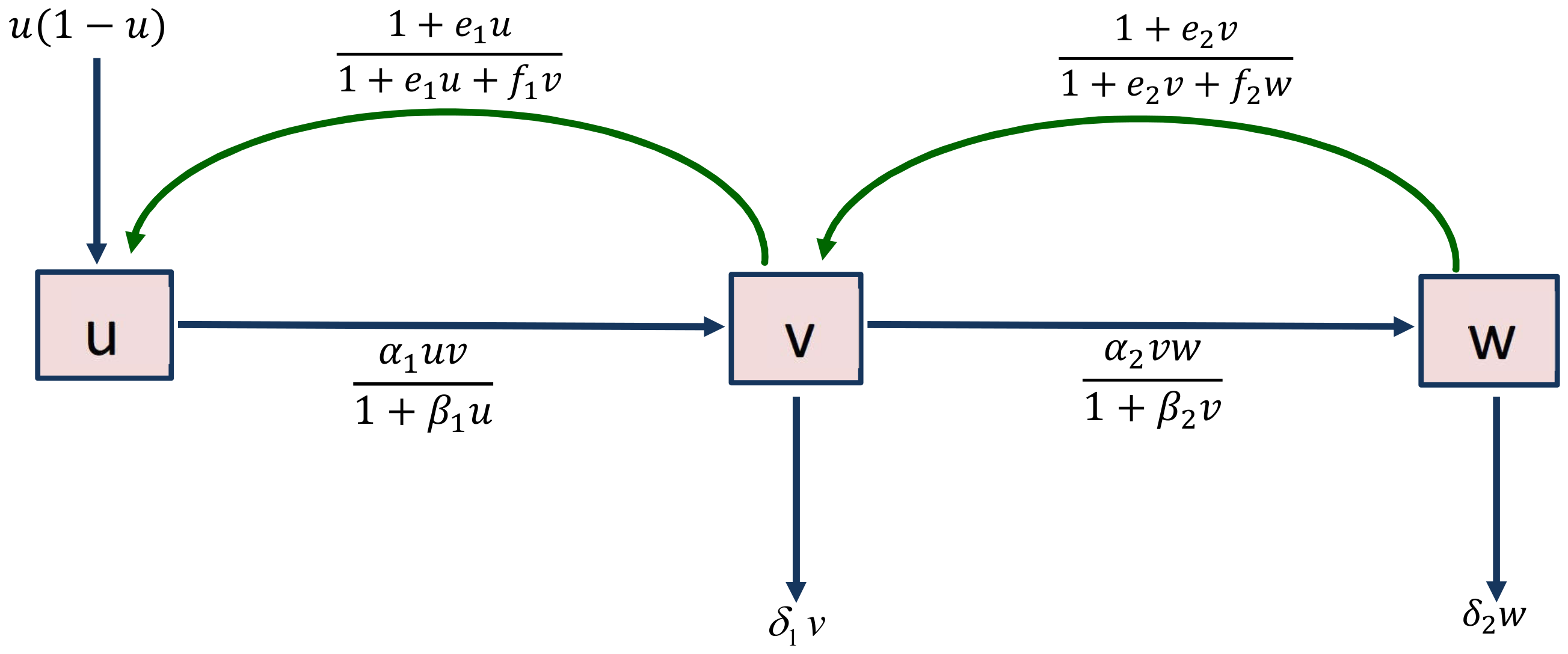3) becomes

$$\begin{array}{c}\hfill \begin{array}{c}{\displaystyle \frac{du}{dt}=u\left({\displaystyle (1-u)·\frac{1+e_{1}u}{1+e_{1}u+f_{1}v}-\frac{{\alpha }_{1}v}{1+{\beta }_{1}u}}\right),}\hfill \\ {\displaystyle \frac{dv}{dt}=v\left({\displaystyle \frac{{\alpha }_{1}u}{1+{\beta }_{1}u}·\frac{1+e_{2}v}{1+e_{2}v+f_{2}w}-\frac{{\alpha }_{2}w}{1+{\beta }_{2}v}-{\delta }_1}\right),}\hfill \\ {\displaystyle \frac{dw}{dt}=w\left({\displaystyle \frac{{\alpha }_{2}v}{1+{\beta }_{2}v}-{\delta }_2}\right)}\hfill \end{array}\end{array}$$

(4)

subject to the initial conditions $0<u_0=u\left(0\right),v_0=v\left(0\right),w_0=w\left(0\right)<\infty$. A conceptual diagram of model (4) is represented in Figure 1.

Figure 1. A conceptual diagram indicates the interaction between the species given in model (4). Here, green lines represent the fear and fear-induced COE on the species.

Remark 1. 

In this paper, we consider the delayed three-species food chain model with fear due to predation and its carry-over effect. If there is no fear-induced carry-over effect (i.e., $e_1=e_2=0$) in the proposed non-delayed model, then the model is reduced to the model studied by Pandey et al. in reference [31]. If there is no fear (i.e., $f_1=f_2=0$) in the proposed non-delayed model, then the model is reduced to the model dealt with by Hastings and Powell [13]. The proposed delayed model was the model discussed by the authors in reference [45] when there is no fear effect on predation growth. The results derived in this paper are general cases of the models investigated in reference [13,31,45]. Panday et al. [33] considered the problem of chaos control in a three-species food chain model by introducing fear to the middle predator only. The chaotic dynamics of the food chain model can be controlled through fear of predation and mutual interference among species [35]. It should be noted that artificially introduced fear plays a crucial role in controllin chaotic dynamics [13,33,35,45]. However, in [13,33,35,45], fear-induced COE is missing, which stimulated the present study. The model proposed in this paper is more applicable in places where there are three-level food chains. Moreover, the model is appropriate to food chain fisheries where the prey includes species, such as yellow perch, sunfish, and herring; the middle predators include species, such as walleye, tuna, and catfish; and the special predators are species, such as sharks, whales, and dolphins.

Remark 2. 

The model proposed in this paper is based on the continuous-time model because the species involved in the system have generations that overlap and births that are spaced throughout the year. By using the standard finite difference schemes, one can obtain discrete-time models from the continuous ones, where the step size represents the generation time. In the absence of middle and special predators in model (4), the prey species grows logistically and the model takes the following form

$$\begin{array}{c}\hfill \begin{array}{c}\frac{dU}{dT}=R_{0}U\left(1-\frac{U}{K}\right).\hfill \end{array}\end{array}$$

(5)

Equation (5) represents a single-species growth model (a logistic model). The discrete version of model (5) tends to be the logistic map, which exhibits a variety of complex behaviors, including unstable, stable, period-doubling, and chaotic oscillations. Chaotic dynamics can be seen in discrete-time models with only one species, but at least three species are needed for continuous-time systems. There has been a lot of research on the dynamical properties, including stability and bifurcation, of both continuous-time models [13,31,43] and discrete-time models [5,6] in independent ways.

3. Preliminaries

Positivity: The positivity of the solution of an ecological model indicates that the density of a population is non-negative at any time.

Theorem 1. 

The solutions of model (4) are positively invariant.

Proof. 

From (4), we have

$$\begin{array}{c}\hfill \begin{array}{c}u\left(t\right)=u\left(0\right)exp\left\{{\displaystyle {\int }_0^t\left[{\displaystyle (1-u\left(s\right))\frac{1+e_{1}u\left(s\right)}{1+e_{1}u\left(s\right)+f_{1}v\left(s\right)}-\frac{{\alpha }_{1}v\left(s\right)}{1+{\beta }_{1}u\left(s\right)}}\right]ds}\right\},\hfill \\ v\left(t\right)=v\left(0\right)exp\left\{{\displaystyle {\int }_0^t\left[{\displaystyle \frac{{\alpha }_{1}u\left(s\right)}{1+{\beta }_{1}u\left(s\right)}\frac{1+e_{2}v\left(s\right)}{1+e_{2}v\left(s\right)+f_{2}w\left(s\right)}-\frac{{\alpha }_{2}w\left(s\right)}{1+{\beta }_{2}v\left(s\right)}-{\delta }_1}\right]ds}\right\},\hfill \\ w\left(t\right)=w\left(0\right)exp\left\{{\displaystyle {\int }_0^t\left[{\displaystyle \frac{{\alpha }_{2}v\left(s\right)}{1+{\beta }_{2}v\left(s\right)}-{\delta }_2}\right]ds}\right\}.\hfill \end{array}\end{array}$$

It should be noted that if any solution is initiated in $R_{+}^3$, then $u\left(t\right),v\left(t\right)$, and $w\left(t\right)$ remain non-negative for all times t. Therefore, $R_{+}^3$ is a positively invariant space for system (4). □

Boundedness: The boundedness of the solution of an ecological model suggests that the model is biologically well-mannered. Additionally, this shows that no species in the biological system experiences sudden or sustained exponential growth. The density of all species is constrained due to the limitation of natural resources.

Theorem 2. 

The solutions $\left(u\right(t),v(t),w(t\left)\right)$ of model (4), which start in the invariant space, are uniformly-bounded.

Proof. 

We define $\Delta \left(t\right)$ as follows

$$\begin{array}{c}\hfill \Delta \left(t\right)=u\left(t\right)+v\left(t\right)+w\left(t\right).\end{array}$$

Time-derivative of $\Delta \left(t\right)$ along with the solutions of model (4); we have

$$\begin{array}{cc}\hfill \frac{d\Delta }{dt}=& \frac{du}{dt}+\frac{dv}{dt}+\frac{dw}{dt}\le u(1-u)-{\delta }_{1}v-{\delta }_{2}w.\hfill \end{array}$$

Then, for any arbitrary constant k, we have

$$\begin{array}{cc}\hfill \frac{d\Delta }{dt}+k\Delta \le & u(1-u+k)-({\delta }_1-k)v-({\delta }_2-k)w\le \frac{{(1+k)}^2}{4}=\Gamma \left(\mathrm{s}\mathrm{a}\mathrm{y}\right),\hfill \end{array}$$

where $k=min\{{\delta }_1,{\delta }_2\}.$ With the help of the differential inequality theory, we have

$$\begin{array}{c}\hfill 0\le \Delta \le \frac{\Gamma (1-e^{-kt})}{k}+\Delta (u\left(0\right),v\left(0\right),w\left(0\right))e^{-kt}.\end{array}$$

Thus, as $t\to \infty$, we obtain $0\le \Delta \le \frac{\Gamma }{k}.$ Thus, solutions $\left(u\right(t),v(t),w(t\left)\right)$ of model (4) that begin in $R_{+}^3-\left\{0\right\}$ are confined in the set $\mathcal{W}=\left\{(u,v,w)\in R_{+}^3:\Delta \le \frac{\Gamma }{k}+ϵ,for any ϵ>0\right\}.$ □

Persistence: Persistence ensures that all interacting species will always coexist at any time, irrespective of the initial population density. Mathematically, it ensures that the population densities of all interacting species are far from zero, and it is defined in the following definition.

Definition 1. 

Model (4) is said to be uniformly persistent if there exist constants $l_i>0,U_i>0,i=1,2,3$, which do not depend on the initial population, and any solution $\left(u\right(t),v(t),w(t\left)\right)$ of model (4) satisfies the following condition:

$$\begin{array}{cc}\hfill 0& <l_1\le \underset{t\to \infty }{lim}infu\left(t\right)\le \underset{t\to \infty }{lim}supu\left(t\right)\le U_1,\hfill \\ \hfill 0& <l_2\le \underset{t\to \infty }{lim}infv\left(t\right)\le \underset{t\to \infty }{lim}supv\left(t\right)\le U_2,\hfill \\ \hfill 0& <l_3\le \underset{t\to \infty }{lim}infw\left(t\right)\le \underset{t\to \infty }{lim}supw\left(t\right)\le U_3.\hfill \end{array}$$

Theorem 3. 

Model (4) is uniformly persistent if ${\alpha }_1>{\delta }_1,$ ${\delta }_1(1+{\beta }_1{l}_1)<{\alpha }_1{l}_1$ and $1-\frac{1}{e_1}<(>){\alpha }_1{l}_2<(>)1-{\alpha }_1{f}_1{l}_2^2$.

Proof. 

From Equation (4), we can obtain

$$\begin{array}{c}\hfill \begin{array}{c}{\displaystyle \frac{du}{dt}\le u(1-u),}\hfill \\ {\displaystyle \frac{dv}{dt}\le v\left({\displaystyle {\alpha }_{1}u-\frac{{\alpha }_{2}w}{1+{\beta }_{2}v}-{\delta }_1}\right),}\hfill \\ {\displaystyle \frac{dw}{dt}\le w\left({\alpha }_{2}v-{\delta }_2\right).}\hfill \end{array}\end{array}$$

Let $U_1,U_2$ and $U_3$ be real positive roots of the following equations $1-u=0$, ${\displaystyle {\alpha }_{1}u-\frac{{\alpha }_{2}w}{1+{\beta }_{2}v}-{\delta }_1=0}$ and ${\alpha }_{2}v-{\delta }_2=0$, respectively. Solving the above equations, we obtain $U_1=1$, $U_2=\frac{{\delta }_2}{{\alpha }_2}$ and $U_3=\frac{({\alpha }_1 - {\delta }_1)({\alpha }_2 + {\beta }_2{\delta }_2)}{{\alpha }_2^2}.$ Utilizing the standard comparison theorem [50], the above inequality gives

$$\begin{array}{c}\hfill \underset{t\to \infty }{lim}supu\left(t\right)\le U_1,\underset{t\to \infty }{lim}supv\left(t\right)\le U_2,\underset{t\to \infty }{lim}supw\left(t\right)\le U_3.\end{array}$$

(6)

Here, $U_1,U_2,U_3$ will be positive if ${\alpha }_1>{\delta }_1.$ Similarly, from Equation (4), one can have

$$\begin{array}{c}\hfill \begin{array}{c}{\displaystyle \frac{du}{dt}\ge u\left({\displaystyle \frac{(1-u)(1+e_{1}u)}{1+e_{1}u+f_{1}v}-{\alpha }_{1}v}\right),}\hfill \\ {\displaystyle \frac{dv}{dt}\ge v\left({\displaystyle \frac{{\alpha }_{1}u}{1+{\beta }_{1}u}\frac{1+e_{2}v}{1+e_{2}v+f_{2}w}-{\alpha }_{2}w-{\delta }_1}\right),}\hfill \\ {\displaystyle \frac{dw}{dt}\ge w\left({\displaystyle \frac{{\alpha }_{2}v}{1+{\beta }_2{U}_2}-{\delta }_2}\right).}\hfill \end{array}\end{array}$$

Let $l_1,l_2,l_3$ be real positive roots of the following equations $\frac{(1 - u)(1 + e_{1}u)}{1 + e_{1}u + f_{1}v}-{\alpha }_{1}v=0$, $\frac{{\alpha }_{1}u}{1 + {\beta }_{1}u}\times \frac{1 + e_{2}v}{1 + e_{2}v + f_{2}w}-{\alpha }_{2}w-{\delta }_1=0$, $\frac{{\alpha }_{2}v}{1 + {\beta }_2{U}_2}-{\delta }_2=0.$ Solving the above equation, we obtain that $l_2=\frac{{\delta }_2(1+{\beta }_2{U}_2)}{{\alpha }_2}$, $l_1$ is the positive root of $e_1{u}^2+({\alpha }_1{l}_2{e}_1+1-e_1)u+{\alpha }_1{l}_2(1+f_1{l}_2)-1=0$ and $l_3$ is the positive root of ${\alpha }_2{f}_2{w}^2+({\alpha }_2(1+e_2{l}_2)+{\delta }_1{f}_2)w+{\delta }_1(1 + e_2{l}_2)-\frac{{\alpha }_1{l}_1(1 + e_2{l}_2)}{1 + {\beta }_1{l}_1}=0.$ Utilizing the standard comparison theorem [50], the above inequality gives that

$$\begin{array}{c}\hfill \underset{t\to \infty }{lim}infu\left(t\right)\ge l_1,\underset{t\to \infty }{lim}infv\left(t\right)\ge l_2,\underset{t\to \infty }{lim}infw\left(t\right)\ge l_3.\end{array}$$

(7)

Here, $l_1,l_2,l_3$ will be positive if either $1-\frac{1}{e_1}<{\alpha }_1{l}_2<1-{\alpha }_1{f}_1{l}_2^2$ or $1-\frac{1}{e_1}>{\alpha }_1{l}_2>1-{\alpha }_1{f}_1{l}_2^2$ and ${\delta }_1(1+{\beta }_1{l}_1)<{\alpha }_1{l}_1.$ Then, by Definition 1 and the inequalities (6)–(7), model (4) is uniformly persistent. □

4. Chaos Control of the Tri-Trophic Food Chain Model

4.1. Existence of Equilibrium Points

We are only interested in feasible equilibrium points because we are investigating an ecological system. The following are possible equilibrium points of model (4).

(i)

The species-free equilibrium $P_0=(0,0,0)$ occurs all of the time.

(ii)

The predator-free equilibrium $P_1=(1,0,0)$ occurs all of the time.

(iii)

The special predator-free equilibrium point $P_2=(u_2,v_2,0),$ where

$$\begin{array}{cc}\hfill u_2=& \frac{{\delta }_1}{{\alpha }_1-{\delta }_1{\beta }_1} \mathrm{and}\hfill \\ \hfill v_2=& \frac{-(1+e_1{u}_2)+\sqrt{{(1+e_1{u}_2)}^2+4{\alpha }_1^{-1}{f}_1(1-u_2)(1+e_1{u}_2)(1+{\beta }_1{u}_2)}}{2f_1}.\hfill \end{array}$$

It is clear that $P_2$ exists only when $0<{\delta }_1<\frac{{\alpha }_1}{1 + {\beta }_1}.$

(iv)

The coexistence equilibrium $P^{\ast }=(u^{\ast },v^{\ast },w^{\ast })$, where $u^{\ast },v^{\ast }$ and $w^{\ast }$ are the positive solution(s) of the equations:

$$\begin{array}{c}\hfill \begin{array}{c}\hfill {\displaystyle \frac{(1-u)(1+e_{1}u)}{1+e_{1}u+f_{1}v}-\frac{{\alpha }_{1}v}{1+{\beta }_{1}u}=0,}\\ \hfill {\displaystyle \frac{{\alpha }_{1}u}{1+{\beta }_{1}u}\frac{1+e_{2}v}{1+e_{2}v+f_{2}w}-\frac{{\alpha }_{2}w}{1+{\beta }_{2}v}-{\delta }_1=0,}\\ \hfill {\displaystyle \frac{{\alpha }_{2}v}{1+{\beta }_{2}v}-{\delta }_2=0.}\end{array}\end{array}$$

(8)

Solving the above equation, we have

$$\begin{array}{c}\hfill v^{\ast }=\frac{{\delta }_2}{{\alpha }_2-{\delta }_2{\beta }_2},\end{array}$$

which is positive when ${\alpha }_2>{\delta }_2{\beta }_2.$ Prey coordinate $u^{\ast }$ is the positive root(s) of the equation

$$\begin{array}{c}\hfill e_1{\beta }_1{u}^3+{\Delta }_1{u}^2+{\Delta }_{2}u+{\Delta }_3=0,\end{array}$$

(9)

where ${\Delta }_1=e_1+{\beta }_1-e_1{\beta }_1,{\Delta }_2={\alpha }_1{e}_1{v}^{\ast }+1-e_1-{\beta }_1$ and ${\Delta }_3={\alpha }_1{v}^{\ast }(1+f_1{v}^{\ast })-1.$ Thus, (9) has no positive roots when ${\Delta }_i>0,i=1,2,3,$ and has at least one positive root if any one of ${\Delta }_i^{{}^{\prime }}$ is negative. The special predator coordinate $w^{\ast }$ is the positive root(s) of the equation

$$\begin{array}{c}\hfill \frac{{\alpha }_2{f}_2}{1+{\beta }_2{v}^{\ast }}{w}^2+\left(\frac{{\alpha }_2(1+e_2{v}^{\ast })}{1+{\beta }_2{v}^{\ast }}+{\delta }_1{f}_2\right)w-(1+e_2{v}^{\ast })\left(\frac{{\alpha }_1{u}^{\ast }}{1+{\beta }_1{u}^{\ast }}-{\delta }_1\right)=0.\end{array}$$

(10)

It is clear from (10) that the sufficient condition for the positive real root of (10) is $\frac{{\alpha }_1{u}^{\ast }}{1 + {\beta }_1{u}^{\ast }}>{\delta }_1.$ This infers that for the survival of the special predator, the number of natural deaths of the middle predators must be less than the critical value.

4.2. Local Stability Analysis

To study the local stability of the equilibrium point, the Jacobian matrix of system (4) at any point $(u,v,w)$ is given by:

$$\begin{array}{c}\hfill J(u,v,w)=\left[\begin{array}{ccc}{j}_{11}& j_{12}& 0\\ j_{21}& j_{22}& j_{23}\\ 0& j_{32}& j_{33}\end{array}\right],\end{array}$$

where

$$\begin{array}{cc}\hfill j_{11}=& {\displaystyle \frac{1-2u+2e_{1}u-3e_1{u}^2}{1+e_{1}u+f_{1}v}-\frac{e_{1}u(1-u)(1+e_{1}u)}{{(1+e_{1}u+f_{1}v)}^2}-\frac{{\alpha }_{1}v}{{(1+{\beta }_{1}u)}^2},}\hfill \\ \hfill j_{12}=& -\frac{f_{1}u(1-u)(1+e_{1}u)}{{(1+e_{1}u+f_{1}v)}^2}-\frac{{\alpha }_{1}u}{1+{\beta }_{1}u},j_{21}=\frac{{\alpha }_1(1+e_{2}v)v}{(1+e_{2}v+f_{2}w){(1+{\beta }_{1}u)}^2},\hfill \\ \hfill j_{22}=& \frac{{\alpha }_{1}u({(1+e_{2}v)}^2+f_{2}w(1+2e_{2}v))}{(1+{\beta }_{1}u)(1+e_{2}v+f_{2}w)}-\frac{{\alpha }_{2}w}{{(1+{\beta }_{2}v)}^2}-{\delta }_1,\hfill \\ \hfill j_{23}=& -\frac{{\alpha }_1{f}_2(1+e_{2}v)uv}{(1+{\beta }_{1}u){(1+e_{2}v+f_{2}w)}^2}-\frac{{\alpha }_{2}v}{(1+{\beta }_{2}v)},j_{32}=\frac{{\alpha }_{2}w}{{(1+{\beta }_{2}v)}^2},j_{33}=\frac{{\alpha }_{2}v}{1+{\beta }_{2}v}-{\delta }_2.\hfill \end{array}$$

Theorem 4. 

The species-free equilibrium $P_0(0,0,0)$ is always not stable.

Proof. 

The eigenvalues of the Jacobian matrix J evaluated at $(0,0,0)$ are $1,-{\delta }_1$ and $-{\delta }_2$. Clearly, 1 is always positive, and $-{\delta }_1$ and $-{\delta }_2$ are always negative. Therefore, the species-free equilibrium $P_0$ is unstable. This result biologically implies long-term surveillance. It means that none of the species will become extinct at the same time. □

Theorem 5. 

The predator-free equilibrium $P_1(1,0,0)$ is LAS if $\frac{{\alpha }_1}{1 + {\beta }_1}<{\delta }_1.$

Proof. 

The eigenvalues of J evaluated at $(1,0,0)$ are $-1,\frac{{\alpha }_1}{1 + {\beta }_1}-{\delta }_1$ and $-{\delta }_2$. Clearly, −1 and $-{\delta }_2$ are always negative and the remaining eigenvalue is negative if $\frac{{\alpha }_1}{1 + {\beta }_1}<{\delta }_1$ holds. Therefore, the predator-free equilibrium point $P_1$ is stable if $\frac{{\alpha }_1}{1 + {\beta }_1}<{\delta }_1,$ otherwise $P_1$ is unstable. It should be noted that if the death rate of the middle predator crosses its critical value ${\delta }_1^c=\frac{{\alpha }_1}{1 + {\beta }_1},$ then predators enter into the extinction stage, and the prey species only survive in the considered model. □

The Jacobian matrix J evaluated at $(u_2,v_2,0)$ is

$$\begin{array}{c}\hfill J(u_2,v_2,0)=\left[\begin{array}{ccc}\overline{j_1}& -\overline{j_2}& 0\\ \overline{j_3}& 0& -\overline{j_4}\\ 0& 0& \overline{j_5}\end{array}\right],\end{array}$$

(11)

where

$$\begin{array}{cc}\hfill \overline{j_1}=& {\displaystyle \frac{1-2u_2+2e_1{u}_2-3e_1{u}_1^2}{1+e_1{u}_2+f_1{v}_2}-\frac{e_1{u}_2(1-u_2)(1+e_1{u}_2)}{{(1+e_1{u}_2+f_1{v}_2)}^2}-\frac{{\alpha }_1{v}_2}{{(1+{\beta }_1{u}_2)}^2},}\hfill \\ \hfill \overline{j_2}=& {\displaystyle \frac{f_1{u}_2(1-u_2)(1+e_1{u}_2)}{{(1+e_1{u}_2+f_1{v}_2)}^2}+\frac{{\alpha }_1{u}_2}{1+{\beta }_1{u}_2},\overline{j_3}=\frac{{\alpha }_1{v}_2}{{(1+{\beta }_1{u}_2)}^2},}\hfill \\ \hfill \overline{j_4}=& {\displaystyle \frac{{\alpha }_1{f}_2{u}_2{v}_2}{(1+{\beta }_1{u}_2)(1+e_2{v}_2)}+\frac{{\alpha }_2{v}_2}{(1+{\beta }_2{v}_2)},\overline{j_5}=\frac{{\alpha }_2{v}_2}{1+{\beta }_2{v}_2}-{\delta }_2.}\hfill \end{array}$$

The characteristic equation of the Jacobian matrix (11) is given by

$$\begin{array}{c}\hfill \left({\lambda }^2-\overline{j_1}\lambda +\overline{j_2}\overline{j_3}\right)(\overline{j_5}-\lambda )=0.\end{array}$$

(12)

Theorem 6. 

The special predator-free equilibrium point $P_2(u_2,v_2,0)$ is LAS if $\overline{j_1}<0$ and $\overline{j_5}<0.$

Proof. 

Note that the roots of the characteristic Equation (12) either have negative or negative real parts if $\overline{j_1}<0$ and $\overline{j_5}<0.$ The special predator-free equilibrium $P_2$ is stable if conditions $\overline{j_1}<0$ and $\overline{j_5}<0$ hold. □

The Jacobian matrix J at $(u^{\ast },v^{\ast },w^{\ast })$ is given by

$$\begin{array}{c}\hfill J\left(P^{\ast }\right)=\left[\begin{array}{ccc}{j}_1& -j_2& 0\\ j_3& j_4& -j_5\\ 0& j_6& 0\end{array}\right],\end{array}$$

(13)

where

$$\begin{array}{cc}\hfill j_1=& {\displaystyle \frac{1-2u^{\ast }+2e_1{u}^{\ast }-3e_1{u}^{\ast 2}}{1+e_1{u}^{\ast }+f_1{v}^{\ast }}-\frac{e_1{u}^{\ast }(1-u^{\ast })(1+e_1{u}^{\ast })}{{(1+e_1{u}^{\ast }+f_1{v}^{\ast })}^2}-\frac{{\alpha }_1{v}^{\ast }}{{(1+{\beta }_1{u}^{\ast })}^2},}\hfill \\ \hfill j_2=& {\displaystyle \frac{f_1{u}^{\ast }(1-u^{\ast })(1+e_1{u}^{\ast })}{{(1+e_1{u}^{\ast }+f_1{v}^{\ast })}^2}+\frac{{\alpha }_1{u}^{\ast }}{1+{\beta }_1{u}^{\ast }},j_3=\frac{{\alpha }_1(1+e_2{v}^{\ast })v^{\ast }}{(1+e_2{v}^{\ast }+f_2{w}^{\ast }){(1+{\beta }_1{u}^{\ast })}^2},}\hfill \\ \hfill j_4=& \frac{{\alpha }_1{e}_2{f}_2{u}^{\ast }{v}^{\ast }{w}^{\ast }}{(1+{\beta }_1{u}^{\ast }){(1+e_2{v}^{\ast }+f_2{w}^{\ast })}^2}+\frac{{\alpha }_2{\beta }_2{v}^{\ast }{w}^{\ast }}{{(1+{\beta }_2{v}^{\ast })}^2},\hfill \\ \hfill j_5=& {\displaystyle \frac{{\alpha }_1{f}_2(1+e_2{v}^{\ast })u^{\ast }{v}^{\ast }}{(1+{\beta }_1{u}^{\ast }){(1+e_2{v}^{\ast }+f_2{w}^{\ast })}^2}+\frac{{\alpha }_2{v}^{\ast }}{(1+{\beta }_2{v}^{\ast })},j_6=\frac{{\alpha }_2{w}^{\ast }}{{(1+{\beta }_2{v}^{\ast })}^2}.}\hfill \end{array}$$

The characteristic equation of (13) is

$$\begin{array}{c}\hfill {\lambda }^3+N_1{\lambda }^2+N_2\lambda +N_3=0,\end{array}$$

(14)

where

$$\begin{array}{c}\hfill N_1=-(j_1+j_4),N_2=j_1{j}_4+j_2{j}_3+j_5{j}_6,N_3=-j_1{j}_5{j}_6.\end{array}$$

Theorem 7. 

The coexistence equilibrium $P^{\ast }(u^{\ast },v^{\ast },w^{\ast })$ is LAS if $N_1>0,N_3>0$, and $N_1{N}_2>N_3$.

Proof. 

We make use of the Routh–Hurwitz (R-H) criterion [51], the equilibrium point $P^{\ast }$ is LAS if $N_1>0,N_3>0$ and $N_1{N}_2>N_3.$ □

Note that when $N_1{N}_2=N_3,$ the system loses its stability around $P^{\ast }$, and the Hopf bifurcation occurs.

4.3. Global Stability Analysis

The Lyapunov function plays a vital role in deriving globally asymptotically stable (GAS) criteria of dynamical systems. Global stability ensures that the state solution will always reach the equilibrium state, regardless of where the initial population begins. We assume that the conditions given in Theorem 3 are well satisfied, which assure the long-term existence of all species involved in system (4). By utilizing Theorems 1 and 2, we define $\overline{\Delta }= \frac{\Delta }{k}$ as a positive constant satisfying $u\left(t\right),v\left(t\right),w\left(t\right)<\overline{\Delta },$ where $0<k\le min\{{\delta }_1,{\delta }_2\}$ and $\Gamma =\frac{{(1+k)}^2}{4}.$ To prove the global stability of $P^{\ast },$ we construct a Lyapunov function L as follows:

$$\begin{array}{c}\hfill L=\left(u-u^{\ast }-u^{\ast }log\frac{u}{u^{\ast }}\right)+\left(v-v^{\ast }-v^{\ast }log\frac{v}{v^{\ast }}\right)+\left(w-w^{\ast }-w^{\ast }log\frac{w}{w^{\ast }}\right).\end{array}$$

Theorem 8. 

The coexistence equilibrium $P^{\ast }(u^{\ast },v^{\ast },w^{\ast })$ is GAS if the condition

$$\begin{array}{cc}\hfill \overline{\Delta }& \left({\alpha }_1{u}^{\ast }+{\alpha }_2{v}^{\ast }\right)+{\delta }_1{v}^{\ast }+{\delta }_2{w}^{\ast }+{\left(\frac{1+u^{\ast }}{2}\right)}^2\le \hfill \\ & \frac{(1+e_1{l}_1)u^{\ast }}{1+(e_1+f_1)\overline{\Delta }}+\frac{{\alpha }_1{l}_1{v}^{\ast }(1+e_2{l}_2)}{(1+{\beta }_1\overline{\Delta })(1+(e_2+f_2)\overline{\Delta })}+\frac{{\alpha }_2{l}_2{w}^{\ast }}{1+{\beta }_2\overline{\Delta }}\hfill \end{array}$$

(15)

holds.

Proof. 

The time derivative of L along the solution of (4) is given by

$$\begin{array}{cc}\hfill \frac{dL}{dt}=& \frac{u-u^{\ast }}{u}\frac{du}{dt}+\frac{v-v^{\ast }}{v}\frac{dv}{dt}+\frac{w-w^{\ast }}{w}\frac{dw}{dt}.\hfill \end{array}$$

(16)

From Equation (4), $\frac{dL}{dt}$ becomes

$$\begin{array}{cc}\hfill \frac{dL}{dt}=& (u-u^{\ast })\left({\displaystyle \frac{(1-u)(1+e_{1}u)}{1+e_{1}u+f_{1}v}-\frac{{\alpha }_{1}v}{1+{\beta }_{1}u}}\right)\hfill \\ & +(v-v^{\ast })\left({\displaystyle \frac{{\alpha }_{1}u}{1+{\beta }_{1}u}\frac{1+e_{2}v}{1+e_{2}v+f_{2}w}-\frac{{\alpha }_{2}w}{1+{\beta }_{2}v}-{\delta }_1}\right)\hfill \\ & +(w-w^{\ast })\left({\displaystyle \frac{{\alpha }_{2}v}{1+{\beta }_{2}v}-{\delta }_2}\right)\hfill \\ \hfill \le & \frac{(u-u^2-u^{\ast }+u{u}^{\ast })(1+e_{1}u)}{1+e_{1}u+f_{1}v}-\frac{{\alpha }_{1}uv}{1+{\beta }_{1}u}+\frac{{\alpha }_{1}u{v}^{\ast }}{1+{\beta }_{1}u}\hfill \\ & +\frac{{\alpha }_{1}uv(1+e_{2}v)}{(1+{\beta }_{1}u)(1+e_{2}v+f_{2}w)}-\frac{{\alpha }_{1}u{v}^{\ast }(1+e_{2}v)}{(1+{\beta }_{1}u)(1+e_{2}v+f_{2}w)}-\frac{{\alpha }_{2}vw}{1+{\beta }_{2}v}\hfill \\ & +\frac{{\alpha }_2{v}^{\ast }w}{1+{\beta }_{2}v}-{\delta }_{1}v+{\delta }_1{v}^{\ast }+\frac{{\alpha }_{2}vw}{1+{\beta }_{2}v}-\frac{{\alpha }_{2}v{w}^{\ast }}{1+{\beta }_{2}v}-{\delta }_{2}w+{\delta }_2{w}^{\ast }\hfill \\ \hfill \le & -\frac{1+e_1{l}_1}{1+(e_1+f_1)\overline{\Delta }}{\left(u-\frac{1+u^{\ast }}{2}\right)}^2+{\left(\frac{1+u^{\ast }}{2}\right)}^2-\frac{(1+e_1{l}_1)u^{\ast }}{1+(e_1+f_1)\overline{\Delta }}+{\alpha }_1\overline{\Delta }{u}^{\ast }\hfill \\ & +{\alpha }_2\overline{\Delta }{v}^{\ast }-\frac{{\alpha }_1{l}_1{v}^{\ast }(1+e_2{l}_2)}{(1+{\beta }_1\overline{\Delta })(1+(e_2+f_2)\overline{\Delta })}-\frac{{\alpha }_2{l}_2{w}^{\ast }}{1+{\beta }_2\overline{\Delta }}+{\delta }_1{v}^{\ast }+{\delta }_2{w}^{\ast }.\hfill \end{array}$$

We observe from the above that $\frac{dL}{dt}\le 0$ if

$$\begin{array}{cc}\hfill {\left(\frac{1+u^{\ast }}{2}\right)}^2& -\frac{(1+e_1{l}_1)u^{\ast }}{1+(e_1+f_1)\overline{\Delta }}+{\alpha }_1\overline{\Delta }{u}^{\ast }+{\alpha }_2\overline{\Delta }{v}^{\ast }-\frac{{\alpha }_2{l}_2{w}^{\ast }}{1+{\beta }_2\overline{\Delta }}\hfill \\ & -\frac{{\alpha }_1{l}_1{v}^{\ast }(1+e_2{l}_2)}{(1+{\beta }_1\overline{\Delta })(1+(e_2+f_2)\overline{\Delta })}+{\delta }_1{v}^{\ast }+{\delta }_2{w}^{\ast }\le 0.\hfill \end{array}$$

That is

$$\begin{array}{cc}\hfill \overline{\Delta }& \left({\alpha }_1{u}^{\ast }+{\alpha }_2{v}^{\ast }\right)+{\delta }_1{v}^{\ast }+{\delta }_2{w}^{\ast }+{\left(\frac{1+u^{\ast }}{2}\right)}^2\le \hfill \\ & \frac{(1+e_1{l}_1)u^{\ast }}{1+(e_1+f_1)\overline{\Delta }}+\frac{{\alpha }_1{l}_1{v}^{\ast }(1+e_2{l}_2)}{(1+{\beta }_1\overline{\Delta })(1+(e_2+f_2)\overline{\Delta })}+\frac{{\alpha }_2{l}_2{w}^{\ast }}{1+{\beta }_2\overline{\Delta }}.\hfill \end{array}$$

We also have $\frac{dL}{dt}=0$ at $P^{\ast }$. As a result of the invariance principle [52], we can conclude that the coexistence equilibrium $P^{\ast }$ is GAS if condition (15) holds. □

The global stability condition of the coexistence equilibrium $P^{\ast }$ given in the above theorem is challenging to infer any ecological justification and, thus, we will verify these results numerically.

4.4. Existence of the Hopf Bifurcation

Here, we establish the conditions of the occurrence of the Hopf bifurcation at equilibrium $P^{\ast }$ by taking $e_2$ as a bifurcation parameter, while other parameters are fixed.

Theorem 9. 

Model (4) experiences the Hopf bifurcation around the interior equilibrium $P^{\ast }$ if there exists a critical value of $e_2,$ say $e_2^{\ast }$, such that

1. 

$N_1\left(e_2^{\ast }\right)N_2\left(e_2^{\ast }\right)-N_3\left(e_2^{\ast }\right)=0,$

2. 

${\left[{\displaystyle \frac{d}{d{e}_2}\left(N_1{N}_2\right)}\right]}_{e_2=e_2^{\ast }}\ne {\left[{\displaystyle \frac{d}{d{e}_2}\left(N_3\right)}\right]}_{e_2=e_2^{\ast }}.$

Proof. 

Let $e_2^{\ast }$ be the critical value of $e_2$, such that

$$\begin{array}{c}\hfill N_1\left(e_2^{\ast }\right)N_2\left(e_2^{\ast }\right)-N_3\left(e_2^{\ast }\right)=0.\end{array}$$

(17)

At $e_2=e_2^{\ast }$, we can rewrite the characteristic Equation (14) as

$$\begin{array}{c}\hfill ({\lambda }^2+N_2)(\lambda +N_1)=0.\end{array}$$

(18)

Note that Equation (18) has root $-N_1$ and purely imaginary roots $\pm i\sqrt{N_2}$, which lead to the existence of the Hopf bifurcation.

We take a point $e_2$ in $(e_2^{\ast }-ϵ,e_2^{\ast }+ϵ)$. Hence, all roots of (16) depend on ${\delta }_2$, namely $p\left(e_2\right)\pm iq\left(e_2\right)$. Some simple calculations yield

$$\begin{array}{c}\hfill \begin{array}{c}\hfill p^3-3p{q}^2+N_1(p^2-q^2)+N_{2}p+N_3=0,\\ \hfill 3p^{2}q-q^3+2N_{1}pq+N_{2}q=0.\end{array}\end{array}$$

(19)

As $q\left(e_2\right)\ne 0,$ from the second equation of (19), it follows that

$$\begin{array}{c}\hfill q^2=3p^2+2N_{1}p+N_2.\end{array}$$

Substituting value $q^2$ into the first equation of (19), we obtain

$$\begin{array}{c}\hfill 8p^3+8N_1{p}^2+2p(N_1^2+N_2)+N_1{N}_2-N_3=0.\end{array}$$

(20)

As $p\left(e_2^{\ast }\right)=0,$ from the above equation, we obtain

$$\begin{array}{c}\hfill {\left[\frac{d\lambda }{d{e}_2}\right]}_{e_2=e_2^{\ast }}=-{\left[\frac{1}{2(N_1^2+N_2)}\frac{d}{d{e}_2}(N_1{N}_2-N_3)\right]}_{e_2=e_2^{\ast }}.\end{array}$$

It is clear from ${\left[\frac{d\lambda }{d{e}_2}\right]}_{e_2=e_2^{\ast }}\ne 0$ that the following condition holds.

$$\begin{array}{c}\hfill {\left[\frac{d}{d{e}_2}(N_1{N}_2-N_3)\right]}_{e_2=e_2^{\ast }}\ne 0.\end{array}$$

Hence, the transversality condition for the existence of the Hopf bifurcation is satisfied. This completes the proof. □

From Theorem 9, it is clear that system (4) undergoes a periodic solution through parameter $e_2.$ Now we will explore the chaos control and direction of the Hopf bifurcating periodic solution by using the theory as discussed in reference [53]. The eigenvectors ${\nu }_1,{\nu }_3$ of the Jacobian matrix $J\left(P^{\ast }\right)$ associated to the eigenvalues ${\lambda }_{1,2}=\pm i\omega$ and ${\lambda }_3=-N_1$, respectively, at $e_2=e_2^{\ast },$ where $\omega =\sqrt{N_2}$, are

$$\begin{array}{c}\hfill {\nu }_1=\left(\begin{array}{c}{s}_{11}-i{s}_{12}\\ s_{21}-i{s}_{22}\\ s_{31}-i{s}_{32}\end{array}\right),{\nu }_3=\left(\begin{array}{c}{s}_{13}\\ s_{23}\\ s_{33}\end{array}\right).\end{array}$$

where

$$\begin{array}{cc}\hfill s_{11}=& s_{13}=1,s_{12}=0,s_{21}=\frac{j_1}{j_2},s_{22}=\frac{\omega }{j_2},s_{23}=\frac{j_1+N_1}{j_2},\hfill \\ \hfill s_{31}=& \frac{j_2{j}_3-{\omega }^2+j_1{j}_4}{j_2{j}_5},s_{32}=\frac{\omega (j_1+j_4)}{j_2{j}_5},s_{33}=-\frac{j_6(j_1+N_1)}{j_2{N}_1}.\hfill \end{array}$$

Now, we make the following transformation $u=u^{\ast }+s_{11}x+s_{12}y+s_{13}z$, $v=v^{\ast }+s_{21}x+s_{22}y+s_{23}z$, $w=w^{\ast }+s_{31}x+s_{32}y+s_{33}z;$ then system (4) reduces to

$$\begin{array}{c}\hfill \begin{array}{c}{\displaystyle \frac{dx}{dt}=\frac{(s_{32}{s}_{23}-s_{22}{s}_{33}){\Psi }_1-s_{32}{\Psi }_2+s_{22}{\Psi }_3}{\Psi }\equiv {\Gamma }_1,}\hfill \\ {\displaystyle \frac{dy}{dt}=\frac{(s_{21}{s}_{33}-s_{23}{s}_{31}){\Psi }_1+(s_{31}-s_{33}){\Psi }_2+(s_{23}-s_{21}){\Psi }_3}{\Psi }\equiv {\Gamma }_2,}\hfill \\ {\displaystyle \frac{dz}{dt}=\frac{(s_{22}{s}_{31}-s_{32}{s}_{21}){\Psi }_1+s_{32}{\Psi }_2-s_{22}{\Psi }_3}{\Psi }\equiv {\Gamma }_3,}\hfill \end{array}\end{array}$$

(21)

where

$$\begin{array}{cc}\hfill \Psi =& s_{32}{s}_{23}-s_{22}{s}_{33}-s_{32}{s}_{21}+s_{22}{s}_{31},\hfill \\ \hfill {\Psi }_1=& (u^{\ast }+s_{11}x+s_{12}y+s_{13}z)(1-u^{\ast }-s_{11}x-s_{12}y-s_{13}z)\hfill \\ & \times \frac{1+e_1(u^{\ast }+s_{11}x+s_{12}y+s_{13}z)}{1+e_1(u^{\ast }+s_{11}x+s_{12}y+s_{13}z)+f_1(v^{\ast }+s_{21}x+s_{22}y+s_{23}z)}\hfill \\ & -\frac{{\alpha }_1(u^{\ast }+s_{11}x+s_{12}y+s_{13}z)(v^{\ast }+s_{21}x+s_{22}y+s_{23}z)}{1+{\beta }_1(u^{\ast }+s_{11}x+s_{12}y+s_{13}z)},\hfill \\ \hfill {\Psi }_2=& \frac{{\alpha }_1(u^{\ast }+s_{11}x+s_{12}y+s_{13}z)(v^{\ast }+s_{21}x+s_{22}y+s_{23}z)}{1+{\beta }_1(u^{\ast }+s_{11}x+s_{12}y+s_{13}z)}\hfill \\ & \times \frac{1+e_2(v^{\ast }+s_{21}x+s_{22}y+s_{23}z)}{1+e_2(v^{\ast }+s_{21}x+s_{22}y+s_{23}z)+f_2(w^{\ast }+s_{31}x+s_{32}y+s_{33}z)}\hfill \\ & -\frac{{\alpha }_2(v^{\ast }+s_{21}x+s_{22}y+s_{23}z)(w^{\ast }+s_{31}x+s_{32}y+s_{33}z)}{1+{\beta }_2(v^{\ast }+s_{21}x+s_{22}y+s_{23}z)}\hfill \\ & -{\delta }_1(v^{\ast }+s_{21}x+s_{22}y+s_{23}z),\hfill \\ \hfill {\Psi }_3=& \frac{{\alpha }_2(v^{\ast }+s_{21}x+s_{22}y+s_{23}z)(w^{\ast }+s_{31}x+s_{32}y+s_{33}z)}{1+{\beta }_2(v^{\ast }+s_{21}x+s_{22}y+s_{23}z)}\hfill \\ & -{\delta }_2(w^{\ast }+s_{31}x+s_{32}y+s_{33}z).\hfill \end{array}$$

The Jacobian matrix of system (21) at $(0,0,0)$ reduces to

$$\begin{array}{c}\hfill J_{(0,0,0)}=\left[\begin{array}{ccc}0& -\omega & 0\\ \omega & 0& 0\\ 0& 0& N\end{array}\right],\end{array}$$

where $N=\frac{\partial {\Gamma }_3}{\partial z}.$ At ${\delta }_2={\delta }_2^{\ast }$ and $(0,0,0)$, we calculate the values of $g_{11}, g_{02}, g_{20}, G_{21},e_{11},$$H_{101}, H_{110}$$e_{20}, \omega , w_{20}, w_{11}$ and $g_{21}$ by using following relations:

$$\begin{array}{cc}\hfill g_{11}=& \frac{1}{4}\left[\frac{{\partial }^2{\Gamma }_1}{\partial x^2}+\frac{{\partial }^2{\Gamma }_2}{\partial y^2}+i\left(\frac{{\partial }^2{\Gamma }_2}{\partial x^2}+\frac{{\partial }^2{\Gamma }_1}{\partial y^2}\right)\right],\hfill \\ \hfill g_{02}=& \frac{1}{4}\left[\frac{{\partial }^2{\Gamma }_1}{\partial x^2}-\frac{{\partial }^2{\Gamma }_1}{\partial y^2}-2\frac{{\partial }^2{\Gamma }_2}{\partial x\partial y}+i\left(\frac{{\partial }^2{\Gamma }_2}{\partial x^2}-\frac{{\partial }^2{\Gamma }_2}{\partial y^2}+2\frac{{\partial }^2{\Gamma }_1}{\partial x\partial y}\right)\right],\hfill \\ \hfill g_{20}=& \frac{1}{4}\left[\frac{{\partial }^2{\Gamma }_1}{\partial x^2}-\frac{{\partial }^2{\Gamma }_1}{\partial y^2}+2\frac{{\partial }^2{\Gamma }_2}{\partial x\partial y}+i\left(\frac{{\partial }^2{\Gamma }_2}{\partial x^2}-\frac{{\partial }^2{\Gamma }_2}{\partial y^2}-2\frac{{\partial }^2{\Gamma }_1}{\partial x\partial y}\right)\right],\hfill \\ \hfill G_{21}=& \frac{1}{8}\left[\frac{{\partial }^3{\Gamma }_1}{\partial x^3}+\frac{{\partial }^3{\Gamma }_1}{\partial x\partial y^2}+\frac{{\partial }^3{\Gamma }_2}{\partial x^2\partial y}+\frac{{\partial }^3{\Gamma }_2}{\partial y^3}+i\left(\frac{{\partial }^3{\Gamma }_2}{\partial x^3}+\frac{{\partial }^3{\Gamma }_2}{\partial x\partial y^2}-\frac{{\partial }^3{\Gamma }_1}{\partial x^2\partial y}+\frac{{\partial }^3{\Gamma }_2}{\partial y^3}\right)\right],\hfill \\ \hfill \omega =& -\frac{\partial {\Gamma }_1}{\partial y},e_{11}=\frac{1}{4}\left(\frac{{\partial }^2{\Gamma }_3}{\partial x^2}+\frac{{\partial }^2{\Gamma }_3}{\partial y^2}\right),e_{20}=\frac{1}{4}\left(\frac{{\partial }^2{\Gamma }_3}{\partial x^2}-\frac{{\partial }^2{\Gamma }_3}{\partial y^2}-2i\frac{{\partial }^2{\Gamma }_3}{\partial x\partial y}\right).\hfill \end{array}$$

We can obtain $w_{11}$ and $w_{20}$ by solving the equations $(\Psi -2i\omega )w_{20}=-e_{20}$ and $N{w}_{11}=-e_{11}.$ Moreover, we have

$$\begin{array}{cc}\hfill H_{110}=& \frac{1}{2}\left[\frac{{\partial }^2{\Gamma }_1}{\partial x\partial z}+\frac{{\partial }^2{\Gamma }_2}{\partial y\partial z}+i\left(\frac{{\partial }^2{\Gamma }_2}{\partial x\partial z}-\frac{{\partial }^2{\Gamma }_1}{\partial y\partial z}\right)\right],\hfill \\ \hfill H_{101}=& \frac{1}{2}\left[\frac{{\partial }^2{\Gamma }_1}{\partial x\partial z}-\frac{{\partial }^2{\Gamma }_2}{\partial y\partial z}+i\left(\frac{{\partial }^2{\Gamma }_2}{\partial x\partial z}+\frac{{\partial }^2{\Gamma }_1}{\partial y\partial z}\right)\right],\hfill \\ \hfill g_{21}=& G_{21}+2H_{110}{w}_{11}+H_{101}{w}_{20}.\hfill \end{array}$$

The following quantities are used to find the direction of the Hopf bifurcation:

$$\begin{array}{cc}\hfill C_1\left(0\right)& {\displaystyle =\frac{i}{2\omega }\left({\displaystyle g_{20}{g}_{11}-2{\left|g_{11}\right|}^2-\frac{{\left|g_{02}\right|}^2}{3}}\right)+\frac{g_{21}}{2},}\hfill \\ \hfill \mu & {\displaystyle =-\frac{Re\left\{C_1\left(0\right)\right\}}{\frac{d}{de}{\left[Re\left({\lambda }_1\left({\delta }_2\right)\right)\right]}_{e_2=e_2^{\ast }}},}\hfill \\ \hfill \beta & =2Re\left\{C_1\left(0\right)\right\},\hfill \\ \hfill T& {\displaystyle =-\frac{Im\left\{C_1\left(0\right)\right\}+{\mu }_2\frac{d}{d{e}_2}{\left[Im\left({\lambda }_1\left({\delta }_2\right)\right)\right]}_{e_2=e_2^{\ast }}}{\omega }.}\hfill \end{array}$$

Note that the sign of $\mu$ indicates the direction of the Hopf bifurcation. If $\mu >0$ (or $\mu <0$), then the Hopf bifurcation is supercritical (or subcritical). The bifurcating periodic solutions are stable (or unstable) if $\beta <0$ (or $\beta >0$). The periods increase (or decrease) if $T>0$ (or $T<0$).

5. Dynamics of the Delayed Food Chain Model

It is well known that to derive a more appropriate real ecological model, time delay is needed. As a result, we modify our proposed model (4) by incorporating the discrete-time lag, $\tau$, which represents the time lag involved in the special predator’s gestation effect. Then, the food chain model becomes

$$\begin{array}{c}\hfill \begin{array}{c}{\displaystyle \frac{du}{dt}=u(1-u)·\frac{1+e_{1}u}{1+e_{1}u+f_{1}v}-\frac{{\alpha }_{1}uv}{1+{\beta }_{1}u},}\hfill \\ {\displaystyle \frac{dv}{dt}=\frac{{\alpha }_{1}uv}{1+{\beta }_{1}u}·\frac{1+e_{2}v}{1+e_{2}v+f_{2}w}-\frac{{\alpha }_{2}vw}{1+{\beta }_{2}v}-{\delta }_{1}v,}\hfill \\ {\displaystyle \frac{dw}{dt}=\frac{{\alpha }_{2}v(t-\tau )w(t-\tau )}{1+{\beta }_{2}v(t-\tau )}-{\delta }_{2}w.}\hfill \end{array}\end{array}$$

(22)

To analyze the stability of system (22), we linearize system (22) around $P^{\ast }$ and obtain

$$\begin{array}{c}\hfill \frac{dY}{dt}=\left[\begin{array}{ccc}{j}_1& -j_2& 0\\ j_3& j_4& -j_5\\ 0& 0& -j_7\end{array}\right]Y\left(t\right)+\left[\begin{array}{ccc}0& 0& 0\\ 0& 0& 0\\ 0& k_1& k_2\end{array}\right]Y(t-\tau ),\end{array}$$

(23)

where

$$\begin{array}{cc}\hfill Y=& {\left[xyz\right]}^T,j_7=-{\delta }_2,k_1=\frac{{\alpha }_2{w}^{\ast }}{{(1+{\beta }_2{v}^{\ast })}^2},k_2=\frac{{\alpha }_2{v}^{\ast }}{1+{\beta }_2{v}^{\ast }},\hfill \end{array}$$

and the remaining $j_i$’s are the same as defined in Theorem 7. We can write the characteristic equation of (23) as follows:

$$\begin{array}{cc}\hfill \overline{D}(\lambda ,\tau )={\lambda }^3+{\theta }_1{\lambda }^2+{\theta }_2\lambda +{\theta }_3+& e^{-\lambda \tau }({\theta }_4{\lambda }^2+{\theta }_5\lambda +{\theta }_6)=0,\hfill \end{array}$$

(24)

where

$$\begin{array}{cc}\hfill {\theta }_1=& j_7-j_1-j_4,{\theta }_2=j_1{j}_4+j_2{j}_3-j_1{j}_7-j_4{j}_7,{\theta }_3=(j_1{j}_4+j_2{j}_3)j_7,\hfill \\ \hfill {\theta }_4=& -k_2,{\theta }_5=j_1{k}_2+j_4{k}_2+j_5{k}_1,{\theta }_6=-(j_1{j}_4+j_2{j}_3)k_2-j_1{j}_5{k}_1.\hfill \end{array}$$

For $\tau >0$, the above equation has infinitely many roots. Putting $\lambda =i\omega (\omega >0)$ in Equation (24), we have

$$\begin{array}{cc}\hfill ({\theta }_1{\omega }^2-{\theta }_3)& =({\theta }_6-{\theta }_4{\omega }^2)cos\left(\omega \tau \right)+{\theta }_5\omega sin\left(\omega \tau \right),\hfill \\ \hfill {\omega }^3-{\theta }_2\omega & ={\theta }_5\omega cos\left(\omega \tau \right)-({\theta }_6-{\theta }_4{\omega }^2)sin\left(\omega \tau \right).\hfill \end{array}$$

Squaring the above equations and then adding them, we have

$$\begin{array}{c}\hfill {\omega }^6+({\theta }_1^2-{\theta }_4^2-2{\theta }_2){\omega }^4+({\theta }_2^2-2{\theta }_1{\theta }_3+2{\theta }_4{\theta }_6-{\theta }_5^2){\omega }^2+({\theta }_3^2-{\theta }_6^2)=0.\end{array}$$

(25)

Substituting ${\omega }^2=\zeta$ in Equation (25), we obtain the following equation:

$$\begin{array}{c}\hfill h\left(\zeta \right)={\zeta }^3+a_1{\zeta }^2+a_2\zeta +a_3,\end{array}$$

(26)

where $a_1={\theta }_1^2-{\theta }_4^2-2{\theta }_2,a_2={\theta }_2^2-2{\theta }_1{\theta }_3+2{\theta }_4{\theta }_6-{\theta }_5^2,a_3={\theta }_3^2-{\theta }_6^2.$ We conclude from Descartes’ rule of sign that if $a_1$ and $a_3$ are of opposite signs, then at least one positive root exists in Equation (26). The condition for the stability switching behavior of $P^{\ast }$ with respect to the delay parameter is given in the following theorem.

Theorem 10. 

Suppose that the equilibrium $P^{\ast }$ is LAS for $\tau =0.$ Let ${\omega }_0^2={\zeta }_0$ be the positive root of (26). Then, there exists $\tau ={\tau }_0$, such that $P^{\ast }$ is stable for $\tau <{\tau }_0,$ and unstable for $\tau >{\tau }_0.$ The system (22) possesses a Hopf bifurcation at $P^{\ast }$ when $\tau ={\tau }_0$ provided $h^{{}^{\prime }}\left(\zeta \right)\ne 0.$

Proof. 

We assume that (26) has ${\zeta }_k,k=1,2,3$ as its roots. Then we have ${\omega }_k=\sqrt{{\zeta }_k},k=1,2,3,$ and the respective threshold value of the time delay ${\tau }_k^j$ is

$$\begin{array}{c}\hfill {\tau }_k^j=\frac{1}{{\omega }_k}arccos\left\{\frac{({\theta }_5-{\theta }_1{\theta }_4){\omega }_k^4+({\theta }_3{\theta }_4-{\theta }_2{\theta }_5+{\theta }_1{\theta }_6){\omega }_k^2-{\theta }_3{\theta }_6}{{\theta }_4{\omega }_k^4+({\theta }_5^2-2{\theta }_4{\theta }_6){\omega }_k^2+{\theta }_6^2}+2\pi j\right\},\end{array}$$

(27)

where $k=1,2,3,j=0,1,\cdots ,$ and define ${\displaystyle {\tau }_0=\underset{k=1,2,3}{min}{\tau }_k^0.}$ Then, ${\tau }_0$ is the first value of $\tau$, such that (24) has a pair of imaginary roots.

In order to utilize the Hopf bifurcation theorem, we need to verify the transversality condition $\mathrm{s}\mathrm{g}\mathrm{n}{\left[\frac{d\Re \left(\lambda \right)}{d\tau }\right]}_{\tau ={\tau }_0}$. Differentiate Equation (24) with respect to $\tau ,$ we have

$$\begin{array}{c}\hfill \frac{d\lambda }{d\tau }=\frac{\lambda ({\theta }_4{\lambda }^2+{\theta }_5\lambda +{\theta }_6)e^{-\lambda \tau }}{3{\lambda }^2+2{\theta }_1\lambda +{\theta }_2+(2{\theta }_4\lambda +{\theta }_5)e^{-\lambda \tau }-\tau ({\theta }_4{\lambda }^2+{\theta }_5\lambda +{\theta }_6)e^{-\lambda \tau }},\end{array}$$

which gives

$$\begin{array}{c}\hfill {\left(\frac{d\lambda }{d\tau }\right)}^{-1}=\frac{3{\lambda }^2+2{\theta }_1\lambda +{\theta }_2+(2{\theta }_4\lambda +{\theta }_5)e^{-\lambda \tau }}{\lambda ({\theta }_4{\lambda }^2+{\theta }_5\lambda +{\theta }_6)e^{-\lambda \tau }}-\frac{\tau }{\lambda }.\end{array}$$

(28)

Now, we have

$$\begin{array}{cc}\hfill \mathrm{s}\mathrm{g}\mathrm{n}{\left[\frac{d\Re \left(\lambda \right)}{d\tau }\right]}_{\tau ={\tau }_0,\lambda =i{\omega }_0}=& \mathrm{s}\mathrm{g}\mathrm{n}{\left[\Re \left(\frac{d\lambda }{d\tau }\right)\right]}_{\tau ={\tau }_0,\lambda =i{\omega }_0}^{-1}=\mathrm{s}\mathrm{g}\mathrm{n}\left[\frac{h^{{}^{\prime }}\left({\zeta }_0\right)}{{\theta }_5^2{\omega }_0^2+{({\theta }_6-{\theta }_4{\omega }_0^2)}^2}\right].\hfill \end{array}$$

Note that ${\theta }_5^2{\omega }_0^2+{({\theta }_6-{\theta }_4{\omega }_0^2)}^2$ is always positive. Then $\left[\frac{d\Re \left(\lambda \right)}{d\tau }\right]$ and $h^{{}^{\prime }}\left({\zeta }_0\right)$ have the same signs. We should note that $h^{{}^{\prime }}\left({\zeta }_0\right)\ne 0$ if Equation (26) has at least one positive root. Hence, the transversality condition is verified. This completes the proof. □

6. Numerical Simulations

In this section, we conduct numerical simulations by using MATLAB and XPPAUT to explore various complex dynamics, including stable, unstable, periodic, and chaotic solutions of the derived model by varying the system parameters. The growth rates of the prey and middle predators will be influenced by the fear and COEs of their predators, which will result in complex dynamics of the food chain model. We should note that the model without the impact of COEs in system (4) is considered in reference [31]. In order to visualize the complex dynamics of the proposed model (4), we present a bifurcation diagram, time trajectories, the largest Lyapunov exponent (LLE), and a phase portrait of the species. The algorithm for calculating LLE is given in Appendix A. All of the parameters except fear and fear-induced COE are chosen from the reference [13]. The ranges for the fear parameter and the fear-induced COE parameter are chosen from [31,43]. We consider the empirical values of the system parameters as follows.

$$\begin{array}{c}\hfill \begin{array}{c}{\alpha }_1=5,{\alpha }_2=0.1,{\beta }_1=3,{\beta }_2=2,{\delta }_1=0.4,{\delta }_2=0.01,f_1=3.5,f_2=0.1,e_1=1.0,e_2=1.0.\end{array}\end{array}$$

(29)

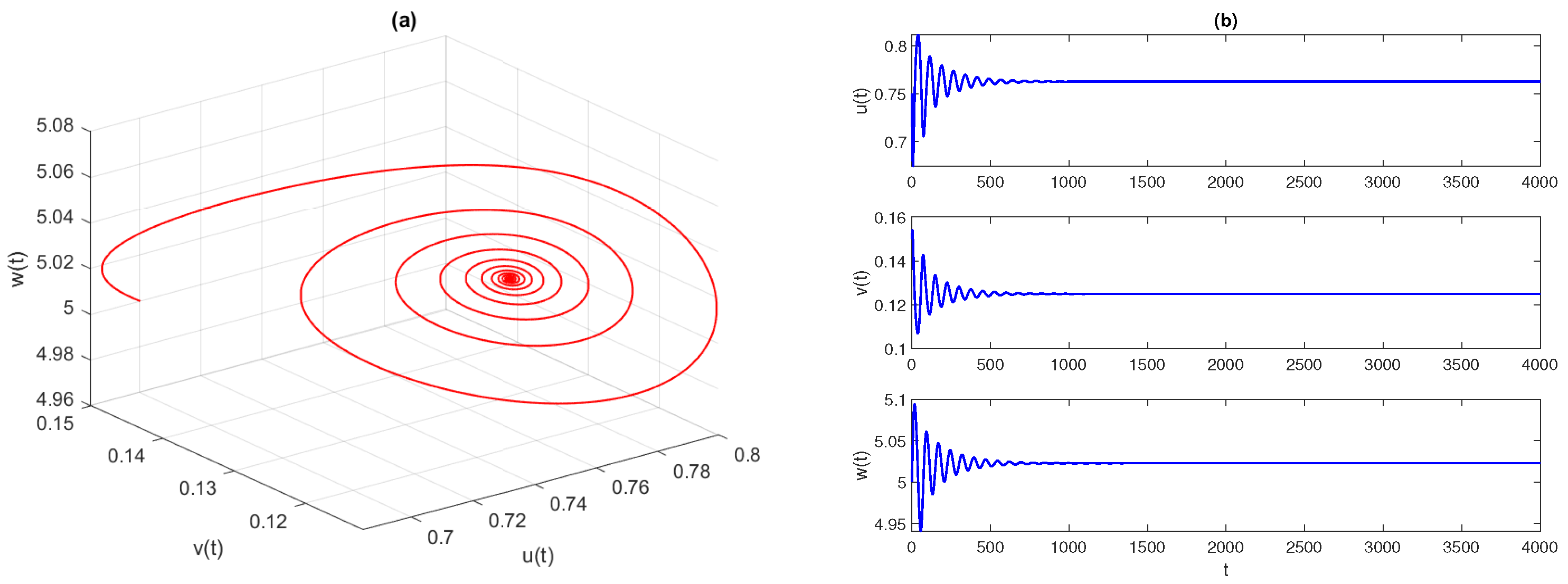
With the parameters given in (29), system (4) having $P_0=(0,0,0),P_1=(1,0,0),P_2=(0.1052,0.1572,0)$ and $P^{\ast }=(0.7627,0.125,5.0228).$ The figures for system (4) are drawn using the initial populations $(0.7,0.1,6)$. Among them, the only coexistence equilibrium point $P^{\ast }$ is stable. Figure 2 displays the phase space diagram and time-series solutions of model (4). They show that solution trajectories converge asymptotically to the stable equilibrium point $P^{\ast }.$ Further, we observe that the equilibrium $P^{\ast }$ is LAS for $e_2=[0,1.361)$. At the critical value of parameters $e_2$, $e_2^{\ast }=1.361$, the equilibrium point $P^{\ast }$ loses its stability and the system experiences a Hopf bifurcation. The conditions given in Theorem 9 are well satisfied, as ${\left[\frac{d}{d{e}_2}\left(N_1{N}_2\right)\right]}_{e_2=e_2^{\ast }}\ne {\left[\frac{d}{d{e}_2}\left(N_3\right)\right]}_{e_2=e_2^{\ast }}$. 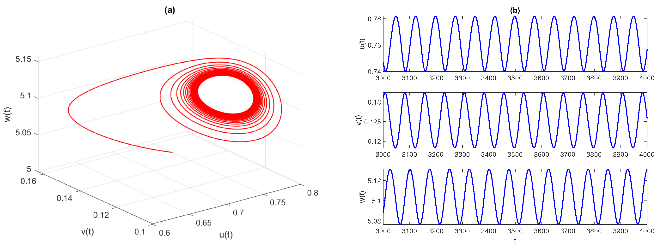In Figure 3, we draw the phase space diagram and time-series solutions of model (4) with $e_2=1.4$ and other parameters as given in Equation (29). Furthermore, we examine the direction and stability properties of positive periodic solutions emerging from the coexistence equilibrium $P\ast$. Applying the results obtained in Section 4.4, we obtain that an occurrence of the Hopf bifurcation is subcritical and the corresponding bifurcating periodic solution is unstable.

Figure 2. Model (4) exhibits stable behavior around the equilibrium point $P\ast$ with the set of values given in (29): (a) phase-space diagram and (b) time trajectories of the solution.

Figure 3. Model (4) exhibits periodic oscillations around the equilibrium point $P\ast$ with the set of values given in (29) except $e_2=1.4>e_2^{\ast }$: (a) phase-space diagram and (b) time trajectories of the solution.

6.1. Impacts of Fear-Induced COEs

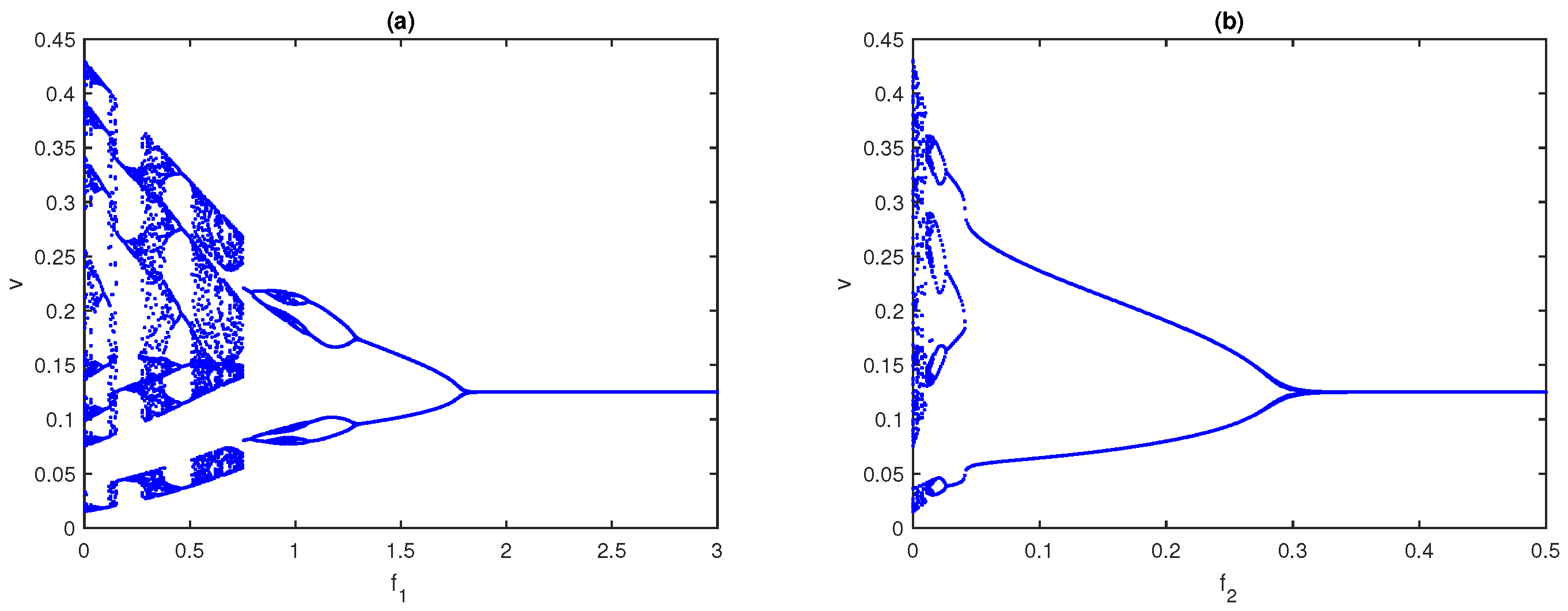
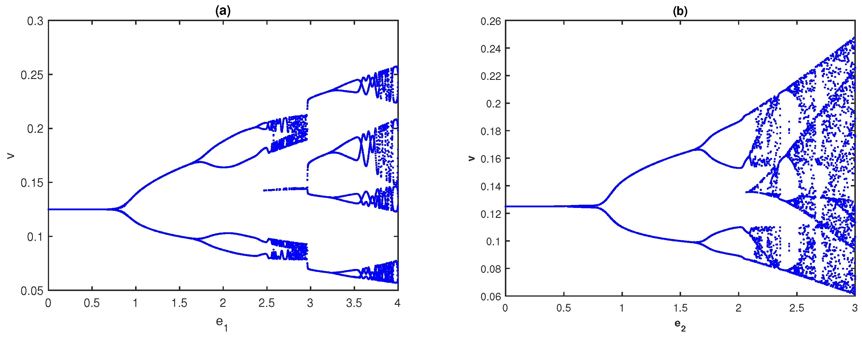
First, we explore the influence of fear in the absence of COEs. The bifurcation diagram of system (4) with respect to $f_1$ in the absence of $f_2$ is presented in Figure 4a, while the bifurcation diagram with respect to $f_2$ in the absence of $f_1$ is given in Figure 4b. It is observed from Figure 4a,b that the system, respectively, approaches a stable state from the chaotic nature through period-halving as fear parameters $f_1$ and $f_2$ increase. When both fear parameters are present, we plot a two-parameter bifurcation diagram in the $f_1-f_2$ parametric plane; see Figure 5. As we can see, for lower values of the $f_1$ and $f_2$ systems, (4) exhibits chaotic behavior and then the system becomes stable for higher values. In an ecological sense, as fear parameters $f_1$ and $f_2$ increase, the growth rate of prey and middle predators decreases, resulting in less prey/middle predators being consumed by middle/special predators. As a result, all three species cannot become extinct in the system but they maintain the positive density. From the above discussions, fear parameters are extremely important in ecology because they may regulate the chaotic nature of the model and make it a stable one. However, the fear of predators also has some COE, which affects the growth rate of respective prey [42].

Figure 4. The bifurcation diagram of the middle predator for model (4): (a) a with respect to $f_1$ when $f_2=0$; (b) with respect to $f_2$ when $f_1=0$. The rest of the system parameters are the same as in Equation (29) except $e_1=0,e_2=0$.

Figure 5. The two-parameter bifurcation diagram for model (4) in the $f_1-f_2$ parametric plane; where the system displays stable behavior in the green region, limit cycle oscillations are in the purple region, period-doubling oscillations are in the yellow region, and chaotic oscillations are in the red region. The rest of the system parameters are the same as in Equation (29) except $e_1=e_2=0$.

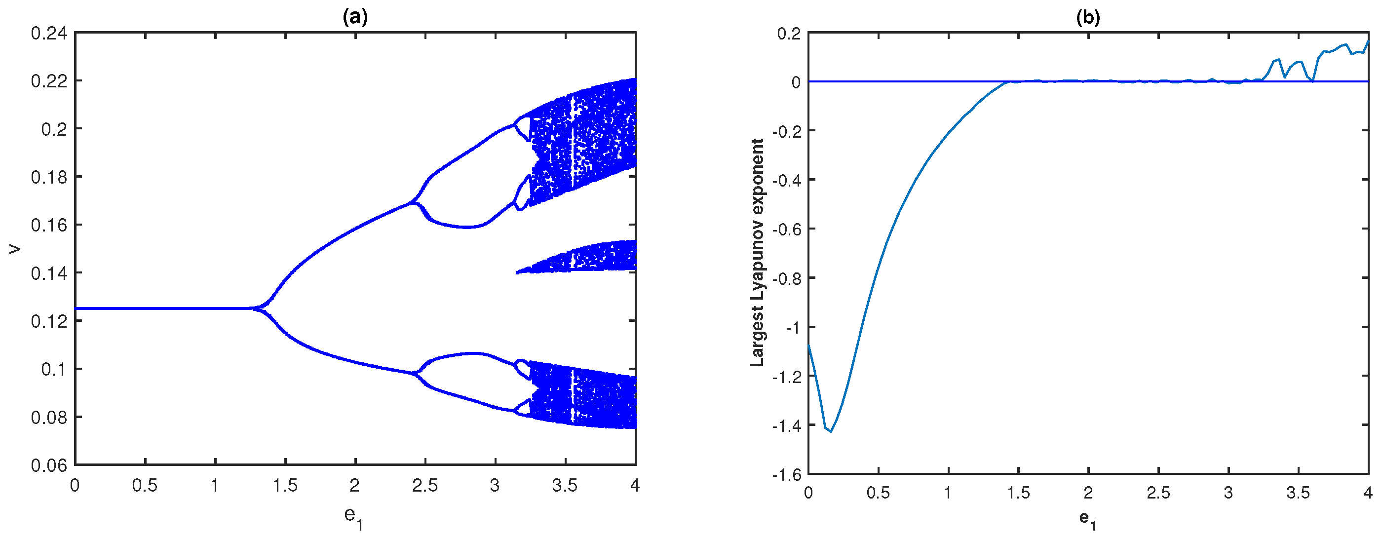
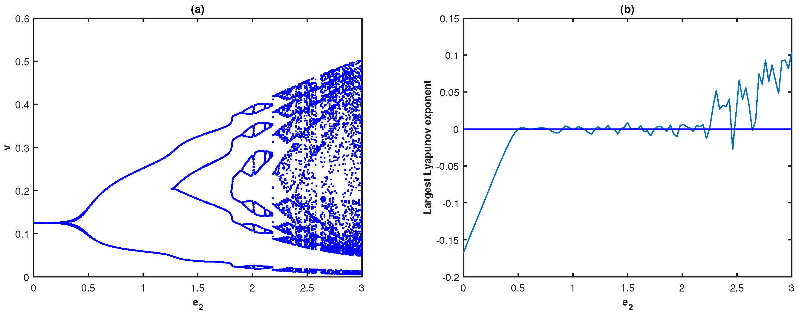
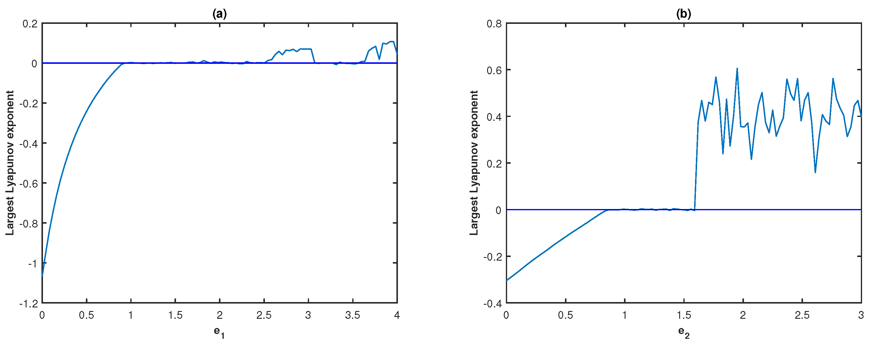
Next, we explore how fear-induced COE parameters are reflected in the system dynamics. First, we analyze the impact of the middle predator induced fear on the prey’s growth and its COE, while the fear of the special predator on the middle predator is absent $(f_2=0)$. The bifurcation diagram and fluctuations of LLE of system (4) with respect to $e_1$ when $f_2=e_2=0$ are, respectively, presented in Figure 6a,b. It can be seen in Figure 6a that the system remains stable for the lower values of $e_1$, then the system turns chaotic through period-doubling as $e_1$ increases. Figure 6a illustrates that the system dynamics demonstrate stable behavior for $e_1<1.27$; limit cycle oscillations for $1.27\le e_1<2.39$, and display higher periodic or chaotic oscillations for $e_1\ge 2.39.$ In addition, we observe that the system remains chaotic for larger values of $e_1.$ To verify the chaotic behavior of system (4), we draw the fluctuation of the LLE with respect to $e_1$ in Figure 6b. 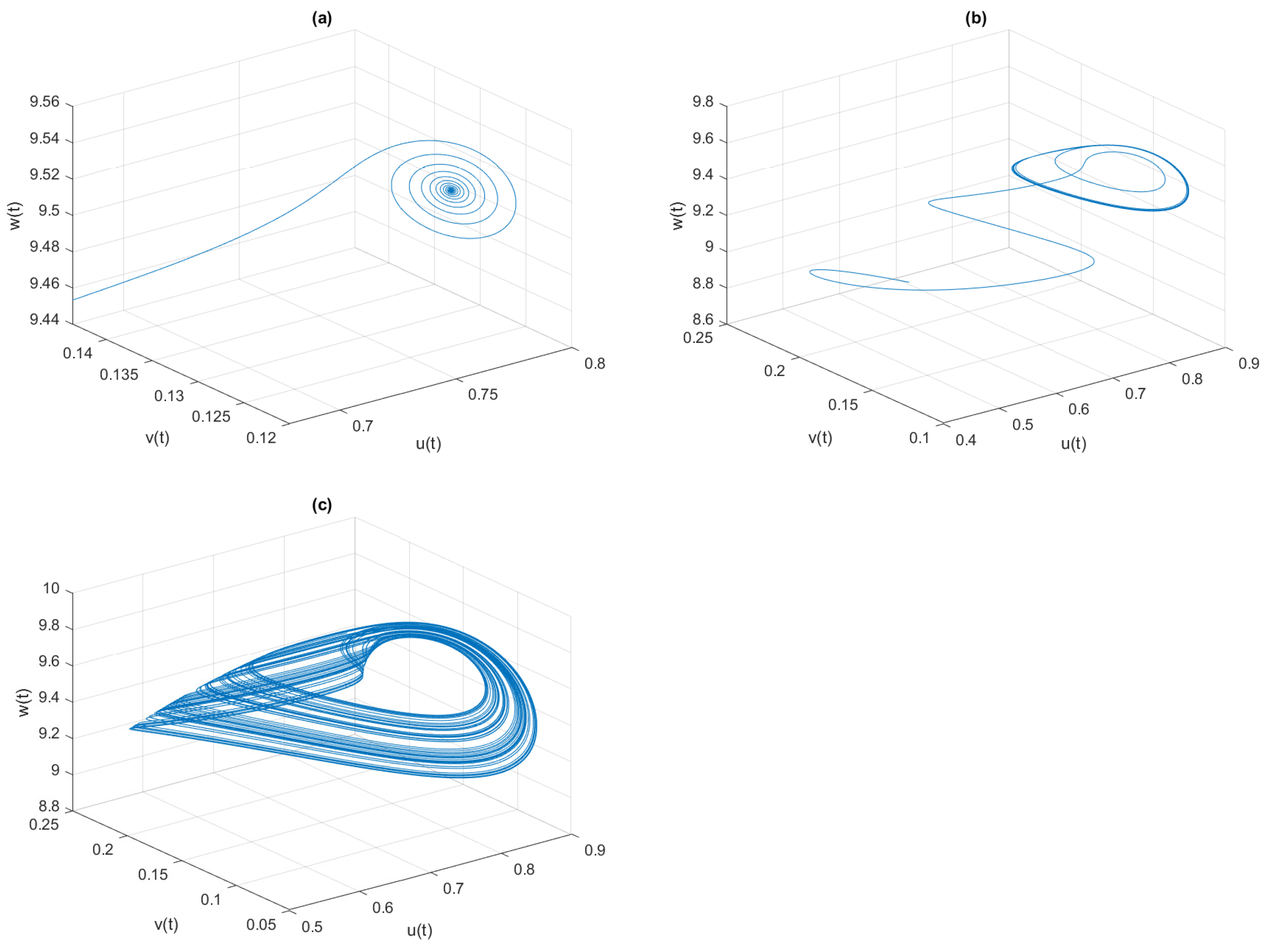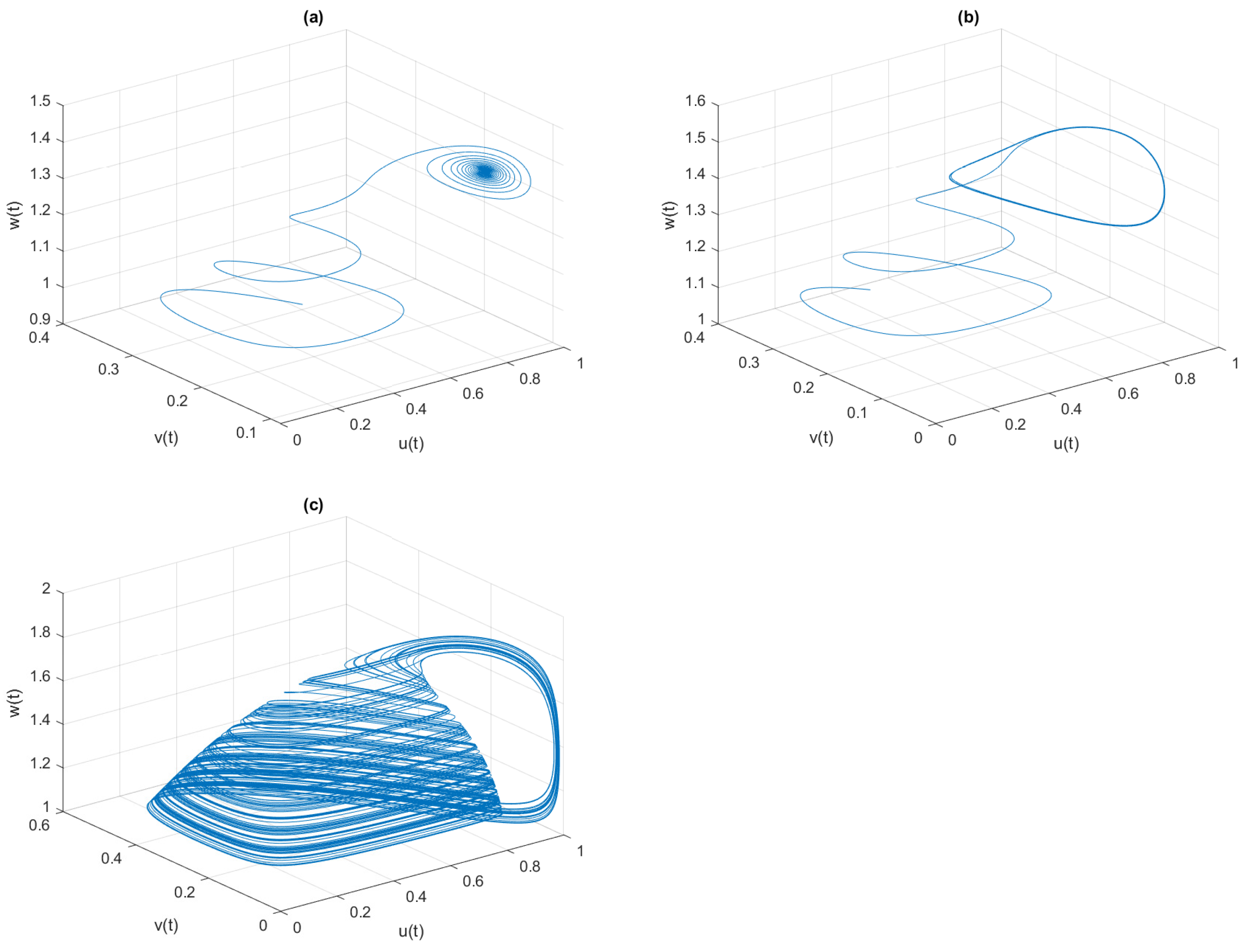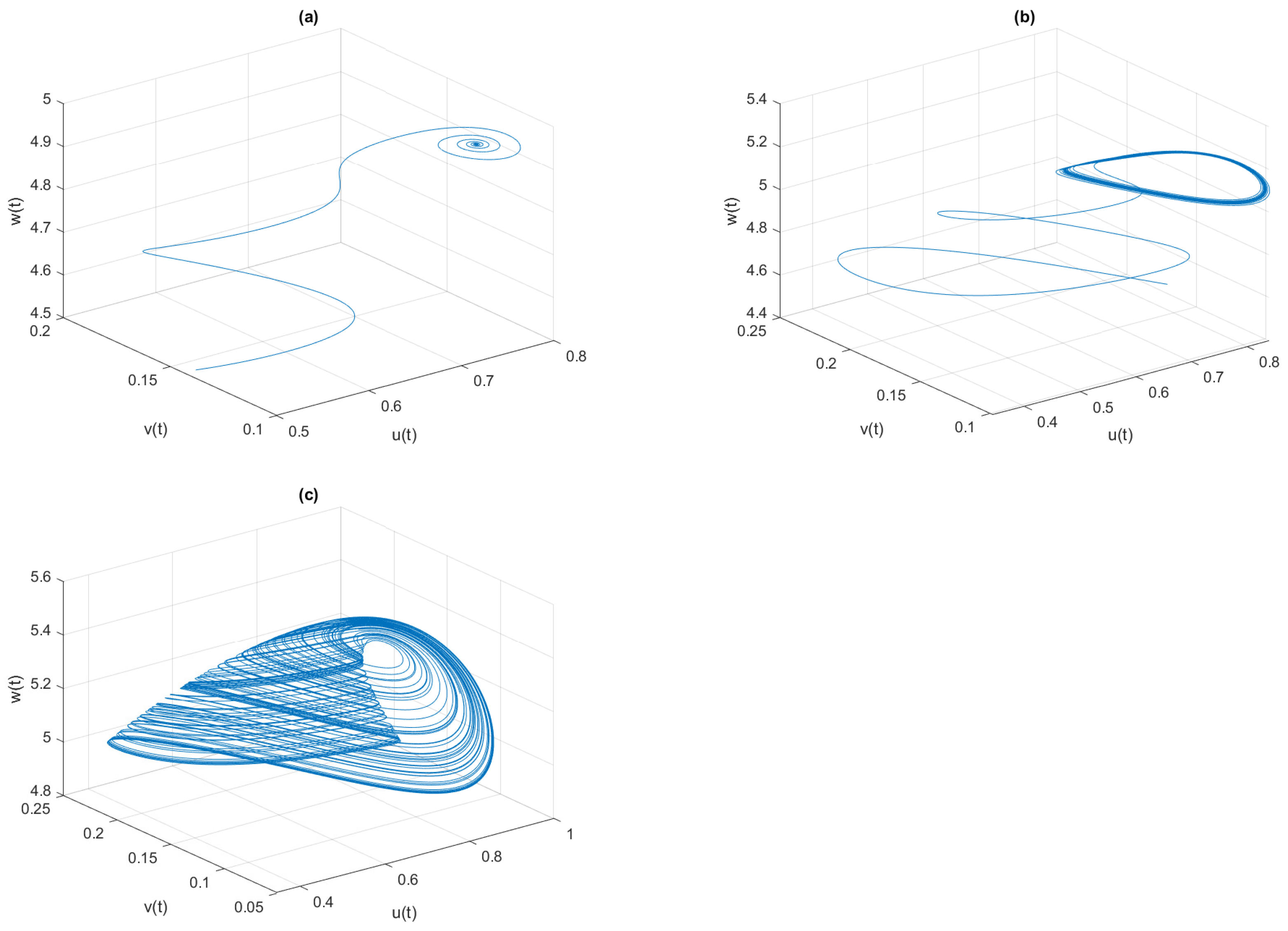For different values of $e_1$, the phase space diagrams of model (4) are given in Figure 7, where the system is LAS for $e_1=1.2$, periodic oscillation for $e_1=2.1$, and chaotic oscillation for $e_1=3.8.$ In Figure 8, we draw a two-parameter bifurcation diagram between fear $f_1$ and its COE parameter $e_1$. For smaller values of $e_1$, we observe that the system changes its state from chaotic oscillation to a stable one through period-halving with $f_1$ increasing, while for higher values, the system remains chaotic. The chaotic phenomena can also be controlled by increasing fear parameter $f_1$. Similarly, we analyze the impact of the special predator-induced fear on the middle predator’s growth and its COE, while the fear of the middle predator on the prey is absent $(f_1=0)$. In this case, Figure 9 displays the bifurcation diagram and LLE of system (4) with respect to $e_2$ when $f_2=1.0.$ We should note that the system becomes chaotic from stable oscillation through period-doubling as COE parameter $e_2$ increases from 0 to 3. The phase space diagrams of model (4) are drawn in Figure 10 for different values of $e_2$, where the system is LAS for $e_2=0.4$, the periodic oscillation is for $e_2=1.0$, and the chaotic oscillation is for $e_2=2.85.$ Moreover, we notice that as $e_2$ further increases, the system enters into periodic oscillation from chaotic oscillation.

Figure 6. For model (4): (a) a bifurcation diagram of the middle predator with respect to $e_1$; (b) fluctuation of the LLE with respect to $e_1$. The rest of the system parameters are the same as in Equation (29) except $f_2=0,c_2=0$.

Figure 7. The phase space diagram of model (4) for different values of $e_1$: (a) LAS for $e_1=1.2$, (b) periodic oscillation for $e_1=2.1$, and (c) chaotic oscillations for $e_1=3.8.$ The rest of the system parameters are the same as in Equation (29) except $f_2=0,c_2=0$.

Figure 8. The two-parameter bifurcation diagram for model (4) in the $e_1-f_1$ parametric plane; where the system displays stable behavior in the green region, limit cycle oscillations are in the purple region, period-doubling oscillations are in the yellow region, and chaotic oscillations are in the red region. The rest of the system parameters are the same as in Equation (29) except $f_2=e_2=0$.

Figure 9. For model (4): (a) a bifurcation diagram of the middle predator with respect to $e_2$; (b) fluctuation of the LLE with respect to $e_2$. The rest of the system parameters are the same as in Equation (29) except $f_1=0,e_1=0,f_2=1.0$.

Figure 10. The phase space diagram of model (4) for different values of $e_2$: (a) LAS for $e_2=0.4$, (b) periodic oscillation for $e_2=1.0$, and (c) chaotic oscillations for $e_2=2.85.$ The rest of the system parameters are the same as in Equation (29) except $f_1=0,c_1=0,f_2=1.0$.

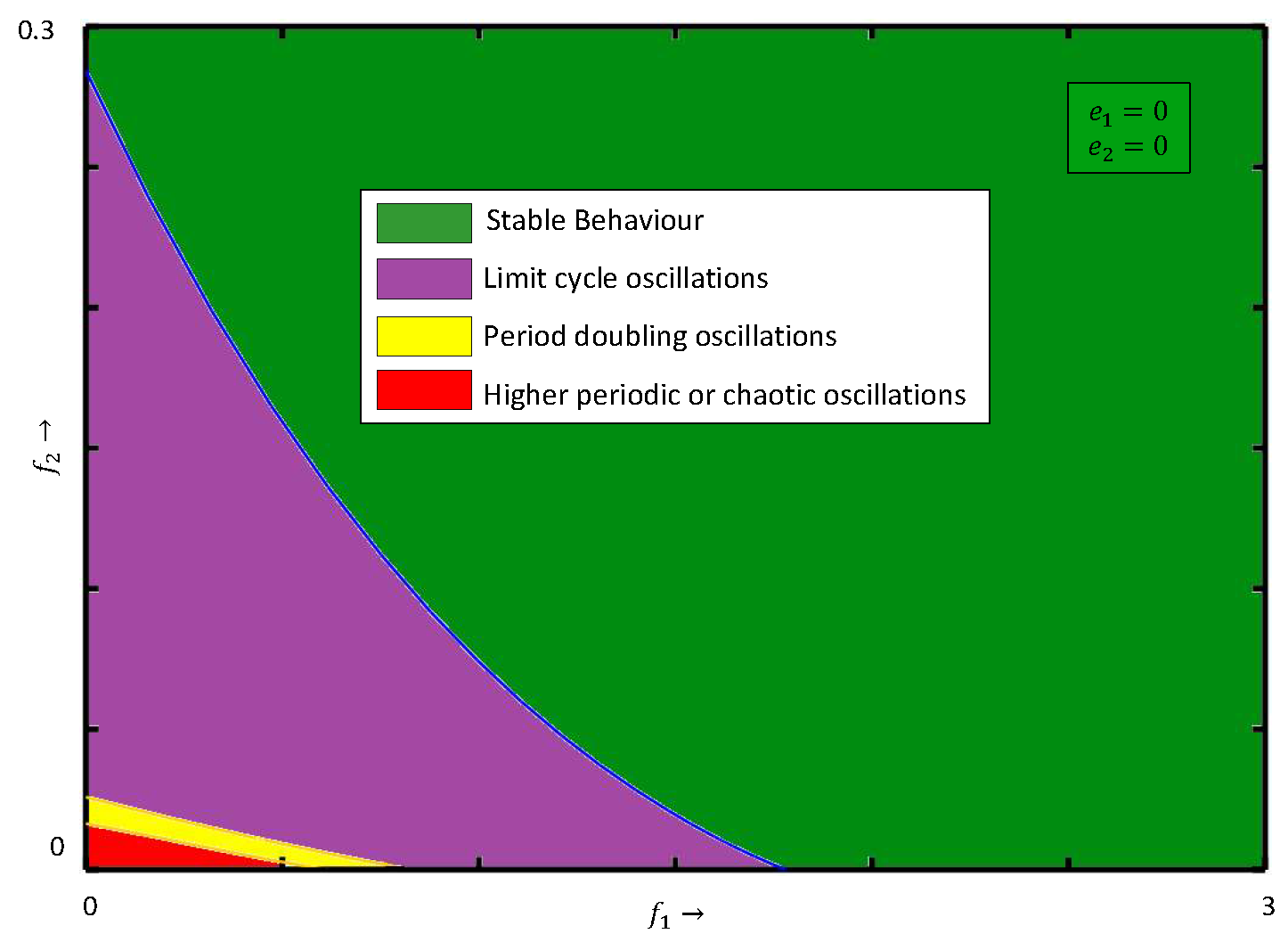
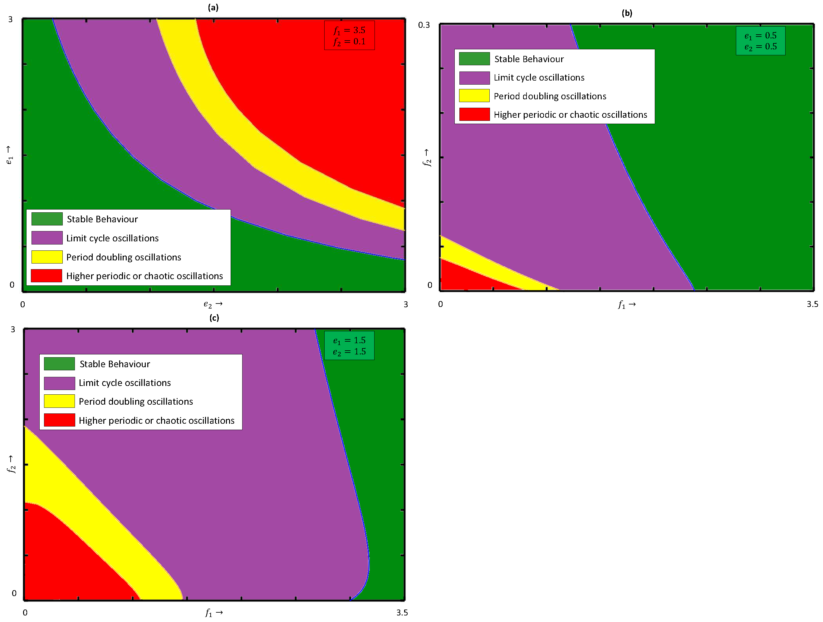
Next, we examine how the system dynamics are influenced when both fear-induced COE factors are present. To emphasize this, we draw the two-parameter bifurcation diagram in the $e_1-e_2$ parametric plane of system (4) in the presence of the fear-induced COE in the prey species as well as in the middle predator, see Figure 11a. We observe that for lower values of COE parameters, $e_1$ and $e_2$, system (4) shows stable behavior and it becomes chaotic through period-doubling as $e_1$ ($e_2$) increases, i.e., both $e_1$ and $e_2$ have destabilizing effects for fixed fear parameters $f_1=3.5,f_2=0.1$. 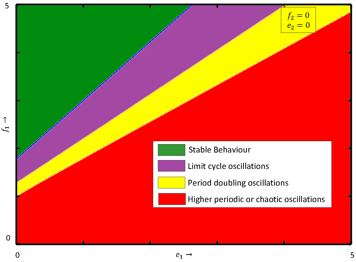Figure 11b,c display the two-parameter bifurcation diagram in the $f_1-f_2$ parametric plane of system (4) with $e_1=e_2=0.5$ and $e_1=e_2=1.5$, respectively. The figure clearly shows that as $e_1$ or $e_2$ increases, the stability region in the $f_1-f_2$ parametric plane gradually decreases. To protect biodiversity, artificially introduced fear through vocalization plays a crucial role. In reality, species learn about the introduced artificial fear from past experiences and pass it on to future generations as fear-induced COE parameters $e_1,e_2,$ increase, and as a result, a greater amount of prey and middle predators are consumed by middle and special predators, respectively, in the ecosystem. This situation leads a species population to an extinction stage. It is clear that the system exhibits chaos for higher values of $e_1,e_2$, and it can be controlled by increasing the fear parameter. For a better understanding of the impacts of $e_1$ and $e_2$ on the dynamics of system (4), we plot the bifurcation diagram with respect to $e_1$ and $e_2$ in Figure 12. It can be observed from Figure 12 that an increase in parameter $e_1$ ($e_2$) makes the system chaotic from stable through period-doubling. If $e_2=1.5,$ we observe that the system exhibits stable behavior for $e_1<0.75$, limits cycle oscillations for $0.75\le e_1<1.75$, and higher periodic or chaotic oscillations for $e_1\ge 1.75.$ Similarly, if $e_1=1.5,$ we observe that the system exhibits stable behavior for $e_1<0.75$, limits cycle oscillations for $0.75\le e_1<1.75$, and higher periodic or chaotic oscillations for $e_1\ge 1.75.$ The chaotic behaviors occurring in Figure 12 can be confirmed by the positive LLE values shown in Figure 13. To show the impacts of parameters $e_1$ and $e_2$ on the system dynamics, we draw the phase space diagrams of model (4) for different values of $e_1$ in Figure 14. The values of LLE presented in Figure 6b, Figure 9b and Figure 13 are summarized in Table 1, where the positive values confirm the chaotic dynamics of model (4).

Figure 11. The two-parameter bifurcation diagram for model (4): (a) $e_1-e_2$ parametric plane; (b,c) $f_1-f_2$ parametric plane; where the system displays stable behavior in the green region, limits cycle oscillations in the purple region, with period-doubling oscillations in the yellow region and chaotic oscillations in the red region. The rest of the system parameters are the same as in Equation (29) except in (a) $f_1=3.5,f_2=0.1,$ (b) $e_1=e_2=0.5,$ (c) $e_1=e_2=1.5$.

Figure 12. The bifurcation diagram of model (4): (a) with respect to $e_1$ when $e_2=1.5,$ (b) with respect to $e_2$ when $e_1=1.5$. The rest of the system parameters are the same as in Equation (29).

Figure 13. The fluctuation of the LLE of model (4): (a) with respect to $e_1$ when $e_2=1.5,$ (b) with respect to $e_2$ when $e_1=1.5$. The rest of the system parameters are the same as in Equation (29).

Figure 14. The phase space diagram of model (4) for different values of $e_2$: (a) LAS for $e_2=0.5$, (b) periodic oscillation for $e_2=1.6$, and (c) chaotic oscillations for $e_2=2.8.$ The rest of the system parameters are the same as in Equation (29).

Table 1. The largest Lyapunov exponent (LLE) for different cases of the food chain model (4).

${\mathit{e}}_1$	LLE		${\mathit{e}}_2$	LLE
	Case ${\mathit{e}}_2=0.0,$	Case ${\mathit{e}}_2=1.5,$		Case ${\mathit{e}}_1=0.0,$	Case ${\mathit{e}}_1=1.5,$
	${\mathit{f}}_{\mathbf{2}}=\mathbf{0}.\mathbf{0}$	${\mathit{f}}_{\mathbf{2}}=\mathbf{0}.\mathbf{1}$		${\mathit{f}}_{\mathbf{1}}=\mathbf{0}.\mathbf{0}$	${\mathit{f}}_{\mathbf{1}}=\mathbf{3}.\mathbf{5}$
$0.0$	$-1.0739$	$-1.0972$	$0.0$	$-0.1672$	$-0.3046$
$0.4$	$-0.9566$	$-0.0332$	$0.3$	$-0.5770$	$-0.1890$
$0.8$	$-0.3694$	$-0.0491$	$0.6$	$-0.0002$	$-0.0830$
$1.2$	$-0.0937$	$-0.0009$	$0.9$	$-0.0008$	$-0.0015$
$1.6$	$0.0013$	$-0.0007$	$1.2$	$-0.0006$	$0.0003$
$2.0$	$0.0032$	$0.0004$	$1.5$	$0.0088$	$-0.0009$
$2.4$	$-0.0034$	$-0.0020$	$1.8$	$0.0037$	$0.4604$
$2.8$	$-0.0018$	$0.0663$	$2.1$	$-0.0035$	$0.3537$
$3.2$	$0.0078$	$0.0003$	$2.4$	$0.0304$	$0.4981$
$3.6$	$0.0017$	$0.0165$	$2.7$	$0.0746$	$0.3790$
$4.0$	$0.1672$	$0.0438$	$3.0$	$0.1044$	$0.3969$
Ref. fig.	Figure 6b	Figure 13a	Ref. fig.	Figure 9b	Figure 13b

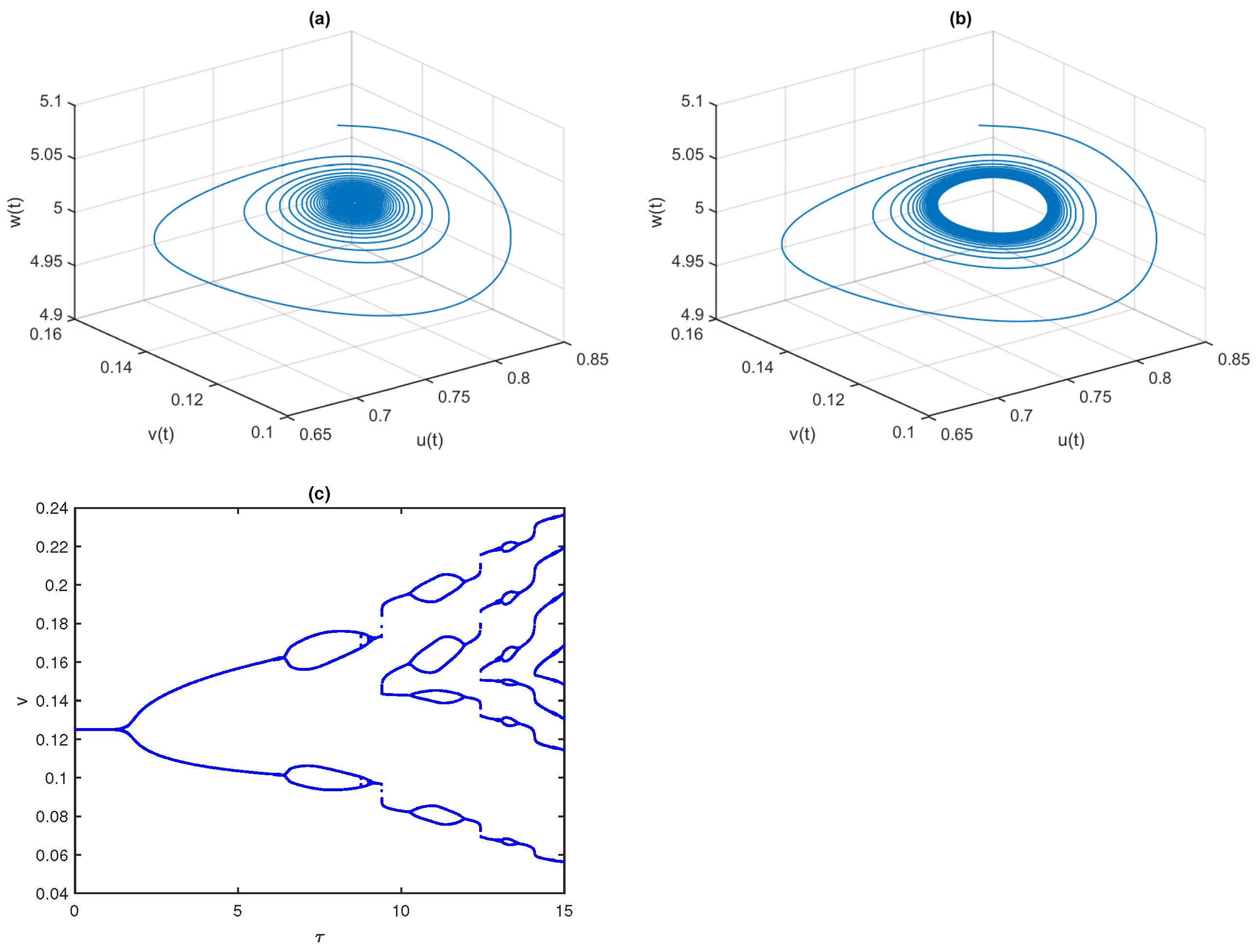
6.2. Effects of Time-Delays

Now, we explore the dynamics of system (22) by varying delay parameters $\tau ,$ and fixing other system parameters as given in (29). We can obtain ${\omega }_0\approx 0.08222$ and critical delay ${\tau }_0\approx 1.7031.$ According to Theorem 10, when $\tau$ passes its critical value ${\tau }_0$, the interior equilibrium $P^{\ast }$ loses its stability and a periodic solution occurs through the Hopf bifurcation, which is given in Figure 15. For low values of $\tau$, the system is in a stable state and then the system loses its stability as $\tau$ passes its critical value. Figure 15c displays the bifurcation diagram of model (22) with respect to $\tau ,$ which indicates that the system (22) is stable for $0\le \tau <1.703$; limit cycle oscillations for $1.703\le \tau <5.8$ and higher periodic or chaotic oscillations for $\tau \ge 5.8.$ Thus, the gestation delay in special predators has a destabilizing effect.

Figure 15. The phase space diagram of model (22): (a) the equilibrium $P^{\ast }$ is LAS for $\tau =1.5<{\tau }_0;$ (b) periodic solution occurs at $\tau =1.85>{\tau }_0.$ (c) The bifurcation diagram of model (22) with respect to $\tau .$ The rest of the system parameters are the same as in Equation (29).

6.3. Discussion

System (4) has four ecologically possible equilibria for system parameters as given in (29). Coexistence equilibrium is the only one that is stable. This means that all solutions to system (4) start with different initial populations that approach equilibrium. In the case without COEs among species, the system becomes stable from its chaotic nature as we increase the fear parameters $f_1$ and $f_2$. Ecologically, middle and special predators can access lower numbers of prey. As a result, none of the species could become extinct in the system while maintaining a positive density level. In the absence of induced fear on the middle predator $f_2=e_2=0$, the system maintains stability for lower values of $e_1$, and the system shows periodic or chaotic oscillations as $e_1$ increases further. Similarly, in the absence of induced fear on the prey, $f_1=e_1=0$, the system transitions from a stable state to a chaotic state as $e_2$ increases and shuttles down in periodic oscillation as $e_2$ increases further. When both fear factors are present constantly, we observe that for lower parameters, $e_1$ and $e_2$, the system shows stable behavior and it becomes chaotic through period-doubling as $e_1$ and/or $e_2$ increase. A greater number of prey and middle predators are consumed by middle and special predators, respectively, in the ecosystem as the COE effect among species increases, and this situation leads to an extinction stage of the species. Thus, both $f_1$ and $f_2$ have stabilizing effects, while both $e_1$ and $e_2$ have destabilizing effects. For a lower time delay, the system is stable. When the time delay increases, the system exhibits higher periodic or chaotic oscillations. The bifurcation diagram of the middle predator is only used because all three species in the system have bifurcation diagrams that are symmetric. To protect biodiversity and manage ecosystems, we can use fear through artificial vocalization.

7. Conclusions

In this work, we investigated the combined impacts of fear and fear-induced carry-over effects (COEs) in the three-species Hastings–Powell model [13]. The Holling type-II functional response is used in the proposed model to describe the asymmetric interference among the species. The growth rates of the prey and middle predator are affected by the respective fears of middle and special predators. Fear and the COE affect the growth rate of the species, which is taken into account in this paper. The preliminaries given in Section 3 ensure that the solution of the proposed system is always positive and non-zero. All ecologically possible equilibriums were evaluated and their local stabilities were analyzed. We further explored the global stability of coexistence equilibrium. We reviewed the Hopf bifurcation at the coexistence equilibrium by taking the middle predator’s COE against the fear of the special predator as a bifurcation parameter. In addition, the proposed model was extended by employing the gestation delay in the special predator growth term, and the Hopf bifurcation was investigated by choosing the time delay as the bifurcation parameter. Lastly, numerical examples were demonstrated to justify the proposed theoretical findings.

Our derived method can be very useful for fishery management. The method proposed in this paper can be extended by incorporating harvesting strategies and Allee effects as well as different functional responses, which will be part of future work.