Chaotic Maps with Tunable Mean Value—Application to a UAV Surveillance Mission ^†

Abstract

Chaos-related applications are abundant in the literature, and span the fields of secure communications, encryption, optimization, and surveillance. Such applications take advantage of the unpredictability of chaotic systems as an alternative to using true random processes. The chaotic systems used, though, must showcase the statistical characteristics suitable for each application. This may often be hard to achieve, as the design of maps with tunable statistical properties is not a trivial task. Motivated by this, the present study explores the task of constructing maps, where the statistical measures like the mean value can be appropriately controlled by tuning the map’s parameters. For this, a family of piecewise maps is considered, with three control parameters that affect the endpoint interpolations. Numerous examples are given, and the maps are studied through a collection of numerical simulations. The maps can indeed achieve a range of values for their statistical mean. Such maps may find extensive use in relevant chaos-based applications. To showcase this, the problem of chaotic path surveillance is considered as a potential application of the designed maps. Here, an autonomous agent follows a predefined trajectory but maneuvers around it in order to imbue unpredictability to potential hostile observers. The trajectory inherits the randomness of the chaotic map used as a seed, which results in chaotic motion patterns. Simulations are performed for the designed strategy.

1. Introduction

1.1. Chaos and Its Applications

Chaotic systems have become standardized tools in applications where a low-cost source of high entropy is required. Examples include secure communications [1], pseudo random bit and number generators [2,3,4,5,6], data encryption [7,8], exploration and surveillance [9,10,11], optimization [12,13,14,15,16], and many more [17]. The reasoning behind their use is that they can generate random-like trajectories, which can be fed into a design to improve its performance. For performance, different indexes can be measured, relevant to the application at hand.

For example, in applications related to data security, like encryption and secure communications [1,2,3,4,5,6,7,8], a chaotic signal is used to hide an information signal. The operations used for hiding include addition between the chaotic series and information, permutation of the information data, and substitution of the data. The resulting encrypted data have a random-like structure, and reveal no information about the original signal. For this, the chaotic signal used should have statistical properties similar to a random process so as to, at least, resist any statistical attacks. So here, uniformity of the chaotic time series chosen is an important and desired feature in assuring the security of the final encrypted data. For an overview of recent developments of chaos-based encryption, see [7,8].

In chaos-based optimization [12,13,14,15,16], and especially in evolutionary algorithms, chaotic time series are used to replace random variables, for actions like selection, emigration, and mutation. The motivation behind this is to replace the uniformity of a random process with a chaotic time series, which is still unpredictable, but may showcase different value distributions on the state space, for different parameter values. So here, the different statistical characteristics of the maps used may improve or hinder the performance of the algorithm, which can then be evaluated by further testing.

In chaotic exploration [9,10,11], an autonomous agent is tasked with either exploring or surveilling a given area of interest. For this, an additional goal is to impart unpredictability in the agent’s path, which can improve the security against intruders and adversaries. For example, the task of trajectory prediction will become hard, making it difficult for an intruder to trespass a secure space. So here, maps with different statistical properties can generate diverse trajectories for the agent to follow.

1.2. Design of New Chaotic Maps

Judging from the collection of diverse examples of chaos-based applications, it is clear that not all of the existing chaotic systems from the vast literature can be utilized in all of the existing applications. Before considering a possible system to use, it is important to not only analyze its dynamical behavior for all control parameters of interest but also consider its statistical behavior. This will facilitate the choosing of the control parameter ranges that will improve the overall performance of the given design.

Motivated by this, the goal of this work is to investigate the changes in the statistical measures of chaotic maps, as their control parameters vary. For this, a simple family of piecewise chaotic maps with three control parameters is proposed. For this family, simple rules can be followed for appropriately tuning the control parameters in order to affect the statistical mean of the resulting time series. Piecewise maps are chosen here, as they are very prominent in applications [3,4,5,18,19,20,21,22,23], and their shape is easy to control. They can also yield chaotic behavior for a wide range of parameter values. Five maps are proposed and studied based on this general model. One map is a generalization of the skewed tent map [20], two are modifications of the maps proposed in [18], and the last two are combinations of the previous ones.

The five chosen maps are analyzed numerically through a collection of tools of nonlinear analysis. First, the bifurcation diagrams and Lyapunov exponents are computed, which are used to identify parameter ranges that yield chaotic behavior. Then, for the parameter ranges that generate chaos, graphs that depict the mean value are generated. These graphs help identify the statistical behavior of the chaotic time series, as the control parameters vary, and follow works that explore the statistical properties of chaotic systems [24,25,26,27].

From all the above studies, the main conclusion is that it is possible to tune the mean value of the proposed maps by appropriately changing the control parameters. This can result in chaotic time series that are left/right-skewed, or closer to a uniform process, all while maintaining unpredictability. Due to the structure of the maps being fairly simple, the tuning guidelines of the control parameters for achieving the desired behavior can be fairly straightforward. Thus, the proposed family of maps can be a starting point for designing maps with controllable statistical measures, all while maintaining wide ranges of chaotic behavior so that the resulting maps can be considered in chaos-based applications.

Another approach to the research problem may be to designate the so-called invariant density. Invariant density shows the distribution of the iterated variable and thus determines basic descriptive statistics, such as the arithmetic mean. This measure can be determined by solving the Frobenius–Perron equation [28]. However, it should be emphasized that in only certain cases (usually mappings composed of linear functions), it is possible to determine this measure analytically. In other cases, this density is approximated by determining histograms.

The problem of finding a mapping with a given density function is thus called the inverse Frobenius–Perron problem (IFPP) [28]. An overview of solutions to this problem can be found in [29]. Such a problem is analyzed, among others, in [30], where the tent map and the cumulative distribution function are used for this purpose. A similar solution using the inverting of the cumulative distribution function is presented in [31]. In turn in [32], a method using stationary densities of dynamical systems with input perturbations is presented. Still, other solutions to this problem can be found in [33,34]. However, it is worth emphasizing that the mentioned solutions of the inverse Frobenius–Perron problem may be ineffective in practical applications.

Motivated by this, the goal of this work is to investigate the changes in the statistical measures of chaotic maps, as their control parameters vary. For this, a simple family of piecewise maps is proposed and analyzed.

To further showcase their applicability, the proposed chaotic maps are applied to the problem of surveillance mentioned above. For this, a scenario is developed where an Unmanned Aerial Vehicle (UAV) follows a predefined trajectory. To introduce chaotic maneuvering into its motion, the chaotic map’s values are utilized to rotate the UAV in a circular region around the predefined trajectory. By performing so, the UAVs trajectory varies as it surveils the area and never repeats itself.

Summarizing, the contributions of this work are outlined as follows:

• A family of piecewise maps with three parameters is proposed. The three parameters are tuned to control the endpoint interpolations.
• By appropriately tuning the control parameters, the statistical mean value of the resulting chaotic time series can be changed.
• The studied maps showcase a collection of dynamical phenomena, including wide uninterrupted parameteric ranges, where chaotic behavior is observed, or self-similar, fractal-like behavior in transitioning in and out of chaos.
• The maps are successfully applied to the problem of the trajectory of a UAV that surveils a given area being imbued with unpredictability.

Finally, it must be noted that this work extends the results of the conference work [35] by studying a wider collection of maps, providing a more in-depth analysis, and the additional application to surveillance. The remainder of the paper is outlined as follows. In Section 2, the family of maps considered here is presented. In Section 3, examples of different maps are presented, and their dynamical behavior is studied. Section 4 presents the chaotic surveillance application. Finally, Section 5 summarizes the paper, with a list of future topics of interest.

2. Proposed Family of Maps

Consider the general family of piecewise maps with two subfunctions of the form

$$x_i=g\left(x_{i-1}\right)=\left\{\begin{array}{cc}{g}_1(x_{i-1},a,b)\hfill & 0\le x_{i-1}\le b\hfill \\ g_2(x_{i-1},b,c)\hfill & b<x_{i-1}\le 1\hfill \end{array}\right.,$$

(1)

with $g\left(x\right)\in [0,1]$, so the mapping interval is $x_i\in [0,1]$. The function $g_1$ is increasing, and $g_2$ is decreasing. The maps (1) have three control parameters $a,b,c\in [0,1]$. These parameters are used to control the shape of the functions $g_1,g_2$ so that they interpolate to the following three points:

$$\begin{array}{ccc}\hfill g_1(0,a,b)& =& a,\hfill \end{array}$$

(2a)

$$\begin{array}{ccc}\hfill g_1(b,a,b)& =& 1,\hfill \end{array}$$

(2b)

$$\begin{array}{ccc}\hfill g_2(1,b,c)& =& c.\hfill \end{array}$$

(2c)

Each subfunction can either be linear or nonlinear, as long as the above conditions hold. These conditions are imposed in order to affect the mapping on the interval $[0,1]$ and change the map’s distribution in the state space. The general rules for tuning each parameter are the following:

• Parameter $a\in [0,1]$. Increasing a affects the mapping interval of the first subfunction to $g_1(x_{i-1},a,b)\in [a,1]$. Thus, the first subfunction will only map to a subset of $[0,1]$, which will result in a skewed distribution of the resulting time series.
• Parameter $b\in [0,1]$. Changing the parameter b will bend the piecewise function g to the left or right, with $b=0.5$ being the symmetric instance. This again can affect the skewness of the resulting time series. For example, increasing the value of $b\in [0.5,1]$, will result in the subfunction $g_1:[0,b]\to [a,1]$ having a wider input domain $[0,b]\supseteq [0,0.5]$, while also mapping to a smaller interval $[a,1]\subseteq [0,1]$, which can result in a right-skewed distribution.
• Parameter $c\in [0,1]$. Increasing c changes the second subfunction to $g_2(x_{i-1},b,c)\in [c,1]$. Similar to $g_1$, this change can affect the distribution of the map, but it can also change the mapping interval of the whole mapping to a subset of $[0,1]$ as will be shown through an example in the next section. Thus, in our upcoming analysis, the parameter c will be set to its default value $c=0$.

The above general rules can be used to design numerous maps, as almost any function can be appropriately mapped to satisfy the conditions (2). Of course, the additional desired property would be to obtain maps that will showcase chaotic behavior for a wide range of parameter values. Such examples are studied next.

3. Considered Maps

In this section, several maps are considered and studied, with respect to the parameters $a,b$. In all cases, the initial condition is fixed to $x_0=0.111$.

3.1. Skewed Tent Map

Based on the well-known skewed tent map [20], the following generalization is proposed:

$$x_i=g\left(x_{i-1}\right)=\left\{\begin{array}{cc}\frac{1-a}{b}{x}_{i-1}+a\hfill & 0\le x_{i-1}\le b\hfill \\ \frac{1-c}{b-1}{x}_{i-1}+\frac{bc-1}{b-1}\hfill & b<x_{i-1}\le 1\hfill \end{array}\right.,$$

(3)

where $a,b,c$ are the map’s parameters. The parameters $a,c$ control the two endpoint interpolations $g\left(0\right)=a$, $g\left(1\right)=c$, and parameter b controls the skew between the two subfunctions.

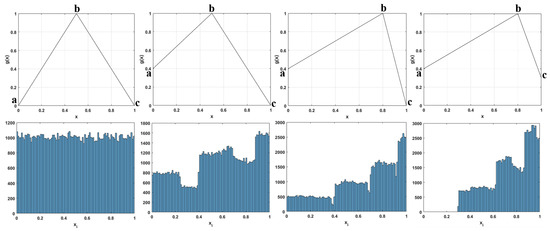
In Figure 1 (top), the function $g\left(x\right)$ is shown for different parameter values. The effect of changing the values of $a,b,c$ on the shape of the curve is clear. As discussed in the previous section, changing the parameters $a,b$ can result in the right-skewness of the resulting time series, while changing c can affect the overall mapping interval. Such examples are shown in Figure 1 (bottom), where the corresponding histograms for ${10}^5$ values of $x_i$ are plotted. This is why in subsequent simulations for all maps, the choice is $c=0$. In the symmetric case $a=0$, $b=0.5001$, the histogram is uniform. When increasing the values of $a,b$, the histogram becomes right-skewed as a result of the first subfunction having a wider domain, and mapping in a smaller interval. So, tuning $a,b$ will have a direct effect on the statistical properties of the time series $\left\{x_i\right\}$. The value of parameter c will be kept to $c=0$, as we want the mapping interval to be $[0,1]$. Note that in the symmetric case, the parameter is set to $b=0.5001$ instead of $b=0.5$ since with complete symmetry, the generalized tent map (3) is identical to the tent map, which falls into periodic behavior due to round-off errors.

Figure 1. (Top) The graph of $g\left(x\right)$ in (3) under different parameters. (Bottom) Corresponding histograms for a time series $x_i$ of the skewed tent map (3) of length ${10}^5$. The parameter values $(a,b,c)$ from left to right are $(0,0.5001,0)$, $(0.4,0.5,0)$, $(0.4,0.8,0)$, $(0.4,0.8,0.3)$.

To gain a first impression of the map’s (3) behavior, its bifurcation diagram is computed. This is shown in Figure 2, with respect to parameter b, and $a=0.5$, $c=0$. The map behaves chaotically in this interval. This diagram gives some insight into the behavior of the map for a fixed a. But since the map has two parameters of interest (the third being fixed $c=0$), a more practical approach is to study its behavior under all possible parameter pairs $(a,b)$, see when the map behaves chaotically, and what is its mean value in each case.

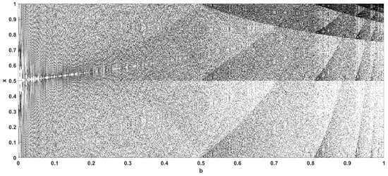
Figure 2. Bifurcation diagram of the skewed tent map (3) with respect to parameter b, for $a=0.5$, and $c=0$. The parameter iteration step is 0.0005.

Thus, to investigate the impact of the parameters $a,b$ on the mean value, the parameter ranges of (3) that generate chaotic behavior are computed. For this, the Lyapunov exponent (LE) of the map is computed for all parameter pairs $(a,b)\in [0,1]\times [0,1]$. The result is shown in Figure 3a, where the colormap corresponds to the LE value achieved, with zero or negative values, that is, the non-chaotic cases, noted in black. The map exhibits chaos for a wide and uninterrupted range of parameter pairs, which is a desirable property, as it can facilitate easier parameter choice.

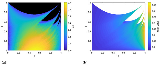
Figure 3. Diagram depicting the LE values (a) and the mean values (b) of the skewed tent map (3) for different values of parameters $a,b$, and $c=0$. The parameter iteration step is 0.0025.

For the parameter pairs that yield chaotic behavior, the diagram in Figure 3b depicts the mean value obtained for a time series of length ${10}^5$. From this diagram, it can be deduced that for lower parameter values, the mean is around 0.5, indicating a uniform histogram. As the parameters take higher values, the mean value also increases, indicating that the histogram of the time series becomes right-skewed. So with this diagram, changes in the statistical behavior of the map can be identified, which are not depicted in either the bifurcation diagram, or the LE diagram.

3.2. Cosine Skewed Piecewise Map

In [18], various piecewise chaotic maps are proposed. Here, one such map is chosen, and a generalized version is proposed as:

$$x_i=g\left(x_{i-1}\right)=\left\{\begin{array}{cc}\frac{f\left(\frac{x_{i-1}}{b}\right)-f\left(0\right)}{f\left(1\right)-f\left(0\right)}+\frac{-a}{b}{x}_{i-1}+a\hfill & 0\le x_{i-1}\le b\hfill \\ \frac{f\left(\frac{x_{i-1}-1}{b-1}\right)-f\left(0\right)}{f\left(1\right)-f\left(0\right)}+\frac{-c}{b-1}{x}_{i-1}+\frac{bc}{b-1}\hfill & b<x_{i-1}\le 1\hfill \end{array}\right.,$$

(4)

where $f\left(x\right)=cos\left(e^{x-1}\right)$. In the original map, the boundaries of the function g were mapped on $g\left(0\right)=0$ and $g\left(1\right)=1$. In the proposed map, $g\left(0\right)=a$ and $g\left(1\right)=c$, so the original map is modified to satisfy conditions (2). A graph of the function g, for $a=0.1$, $b=0.8$, $c=0.2$, is shown in Figure 4. In contrast to the tent map (3), each subfunction is now nonlinear. The functions are also convex.

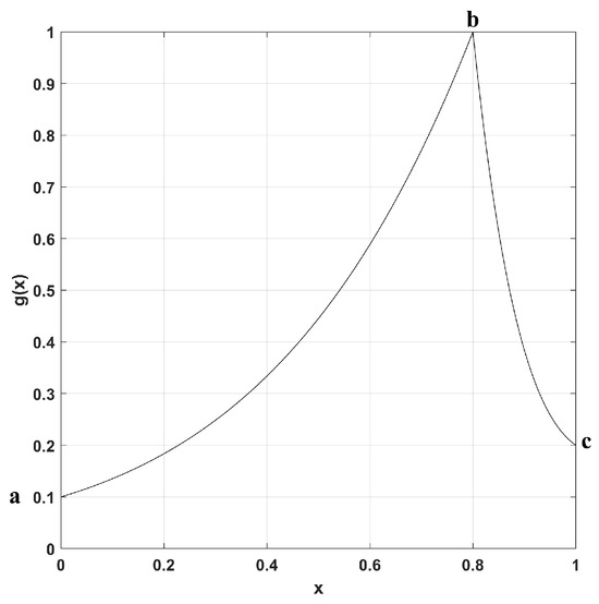
Figure 4. The function $g\left(x\right)$ of the map of (4), with $f\left(x\right)=cos\left(e^{x-1}\right)$, for $a=0.1$, $b=0.8$, and $c=0.2$.

Figure 5 shows the bifurcation diagram of the map with respect to parameter b, and $a=0.5$, $c=0$. The map shows a very intricate behavior, as it traverses in and out of chaos, following a period-doubling cascade, or a period-halving behavior. More impressively, we can observe multiple patterns of period-halving transition from chaos for lower values of b, and period-doubling transitions to chaos for higher values of b. A detailed view of this is shown in Figure 6 as well. This complex self-similar, fractal-like behavior will also be visible in the LE graphs shown next.

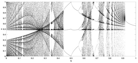
Figure 5. Bifurcation diagram of the map (4), with $f\left(x\right)=cos\left(e^{x-1}\right)$, with respect to parameter b, for $a=0.5$ and $c=0$. The parameter iteration step is 0.0005.

Figure 6. Detailed view of the bifurcation diagram of the map (4) showin in Figure 5, with $f\left(x\right)=cos\left(e^{x-1}\right)$, with respect to parameter $b\in [0,0.2]$, for $a=0.5$ and $c=0$.

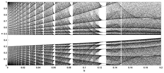
Figure 7a shows the LE value achieved for each parameter pair. Most parameter pairs generate chaos, but now there are non-chaotic regions appearing, which have a fractal-like structure, the so-called “shrimps”. Figure 7b depicts the mean value of the time series for the parameter pairs that generate chaos. Lower and higher values are both achieved, so the histogram shifts from left- to right-skewed.

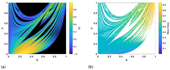
Figure 7. Diagram depicting the LE values (a) and mean values (b) of the map (4), with $f\left(x\right)=cos\left(e^{x-1}\right)$, for different values of parameters $a,b$, and $c=0$. The parameter iteration step is 0.0025.

3.3. Secant Skewed Piecewise Map

An additional variation of Equation (4) is also studied, with the nonlinear function chosen as $f\left(x\right)=\sec \left(e^{x-1}\right)$. Figure 8 shows the graph of $g\left(x\right)$ for $a=0.1$, $b=0.8$, and $c=0.2$. The functions are again convex in shape.

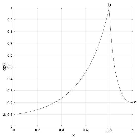
Figure 8. The function $g\left(x\right)$ of the map (4), with $f\left(x\right)=\sec \left(e^{x-1}\right)$, for $a=0.1$, $b=0.8$, $c=0.2$.

Figure 9 shows the bifurcation diagram of the map with respect to parameter b, and $a=0.5$ and $c=0$. As with the previous map, this map also showcases intricate self-similar, fractal-like behavior in its transitions to and from chaos. As parameter b increases, the map falls into a period-1 behavior.

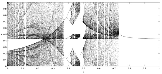
Figure 9. Bifurcation diagram of the map (4), with $f\left(x\right)=\sec \left(e^{x-1}\right)$, with respect to parameter b, for $a=0.5$ and $c=0$. The parameter iteration step is 0.0005.

As with previous maps, Figure 10a depicts the LE values for all parameter pairs $(a,b)$. The chaotic regions follow a pattern similar to the Cosine Skewed Piecewise Map, with non-chaotic, self-similar fractal-like patterns appearing. For the chaotic regions, in Figure 10b, it can be observed that similar to the previous map, the mean value ranges from around 0.2 up to 0.8.

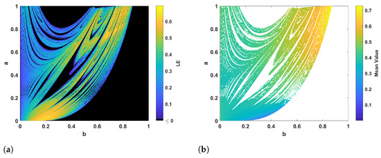
Figure 10. Diagram depicting the LE values (a) and mean values (b) of the map (4), with $f\left(x\right)=\sec \left(e^{x-1}\right)$, for different values of parameters $a,b$, and $c=0$. The parameter iteration step is 0.0025.

3.4. Tent-Cosine Skewed Piecewise Map

Combining the previous maps, two combinations can be derived. The first map is the Tent-Cosine Skewed Piecewise Map, described by

$$x_i=g\left(x_{i-1}\right)=\left\{\begin{array}{cc}\frac{1-a}{b}{x}_{i-1}+a\hfill & 0\le x_{i-1}\le b\hfill \\ \frac{f\left(\frac{x_{i-1}-1}{b-1}\right)-f\left(0\right)}{f\left(1\right)-f\left(0\right)}+\frac{-c}{b-1}{x}_{i-1}+\frac{bc}{b-1}\hfill & b<x_{i-1}\le 1\hfill \end{array}\right.,$$

(5)

where $f\left(x\right)=cos\left(e^{x-1}\right)$. So the first subfunction is taken from the tent map (3), while the second subfunction is taken from (4). The plot of this function in Figure 11 makes this clear.

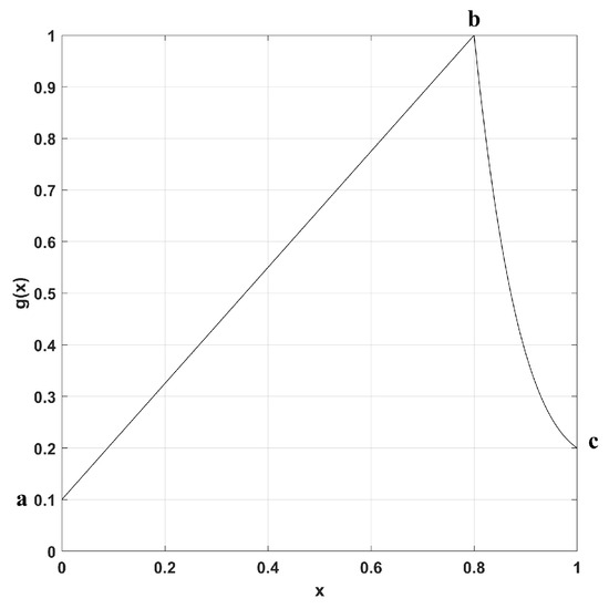
Figure 11. The function $g\left(x\right)$ of the map (5), with $f\left(x\right)=\cos \left(e^{x-1}\right)$, for $a=0.1$, $b=0.8$, and $c=0.2$.

Figure 12 shows the bifurcation diagram of the map with respect to parameter b, and $a=0.5$, $c=0$. The map shows wide regions of chaotic behavior, similar to the tent map (3). As parameter b increases, patterns of transition between chaos and periodic behavior start to emerge, as will be more evident from the next Figure 13a.

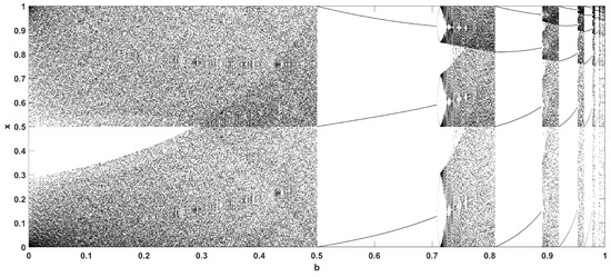
Figure 12. Bifurcation diagram of the map (5), with $f\left(x\right)=\cos \left(e^{x-1}\right)$, with respect to parameter b, for $a=0.5$, $c=0$. The parameter iteration step is 0.0005.

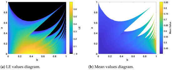
Figure 13. Diagram depicting the LE values (a) and mean values (b) of the map (5), with $f\left(x\right)=\cos \left(e^{x-1}\right)$, for different values of parameters $a,b$, and $c=0$. The parameter iteration step is 0.0025.

The diagram of LE values for the map (5) is shown in Figure 13a. Here, it can be observed that the behavior of this hybrid map is similar to that of the tent map (3) shown in Figure 3a, as the map exhibits wide parameter ranges of uninterrupted chaotic behavior, in contrast to the rest of the maps that exhibited self-similar, fractal-like, non-chaotic regions.

The same similarity between the tent map (5) also holds for the mean value. In Figure 13b, it can be seen that the map’s behavior ranges from a mean of around 0.5, to higher values of around 0.85, which is similar to the behavior shown in Figure 3b.

3.5. Cosine-Tent Skewed Piecewise Map

The second combination considered is the Cosine-Tent Skewed Piecewise Map, described by

$$x_i=g\left(x_{i-1}\right)=\left\{\begin{array}{cc}\frac{f\left(\frac{x_{i-1}}{b}\right)-f\left(0\right)}{f\left(1\right)-f\left(0\right)}+\frac{-a}{b}{x}_{i-1}+a\hfill & 0\le x_{i-1}\le b\hfill \\ \frac{1-c}{b-1}{x}_{i-1}+\frac{bc-1}{b-1}\hfill & b<x_{i-1}\le 1\hfill \end{array}\right.,$$

(6)

where $f\left(x\right)=cos\left(e^{x-1}\right)$. So the first subfunction is taken from (4), while the second subfunction is taken from the tent map (3). The graph of the function shown in Figure 14 illustrates this.

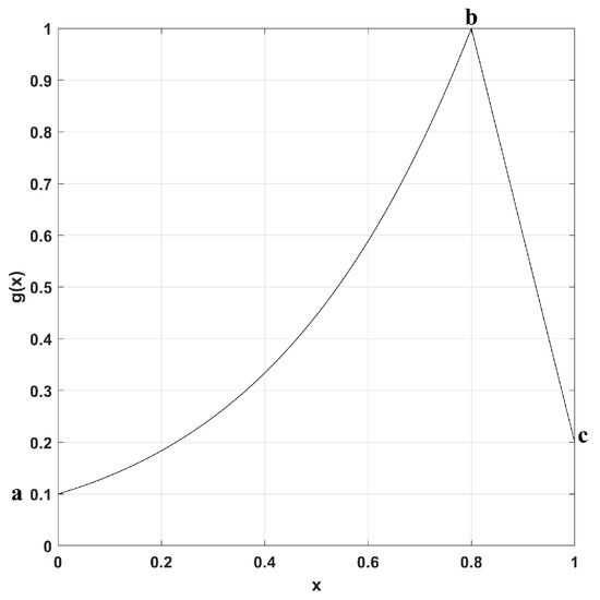
Figure 14. The function $g\left(x\right)$ of the map (6), with $f\left(x\right)=\cos \left(e^{x-1}\right)$, for $a=0.1$, $b=0.8$, $c=0.2$.

Figure 15 shows the bifurcation diagram of the map with respect to parameter b, and $a=0.5$ and $c=0$. This map is more similar to the modified map (4), as it shows self-similar, fractal-like patterns in its transitions to and from chaos, with a period-1 behavior emerging for higher values of b.

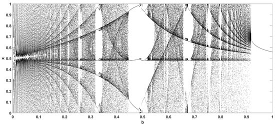
Figure 15. Bifurcation diagram of the map (6), with $f\left(x\right)=\cos \left(e^{x-1}\right)$, with respect to parameter b, for $a=0.5$, $c=0$. The parameter iteration step is 0.0005.

The chaotic behavior and statistical behavior of this map are more similar to the modified map (4). Its chaotic regions shown in Figure 16a showcase periodic interruptions of the fractal-like shape, and the mean value shown in Figure 16b ranges from low to high values. Comparing these two hybrid maps (5) and (6), it seems that the first subfunction is more influential to the behavior of the map.

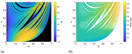
Figure 16. Diagram depicting the LE values (a) and mean values (b) of the map (6), with $f\left(x\right)=\cos \left(e^{x-1}\right)$, for different values of parameters $a,b$, and $c=0$. The parameter iteration step is 0.0025.

3.6. Discussion

From the five different maps considered, rich dynamics were observed overall. The Skewed Tent map (3) and Tent-Cosine map (5) exhibited wider regions of uninterrupted chaotic behavior in contrast to the other three maps. They can thus be considered more suitable for applications, as their acceptable parameter range is easier to define. The Cosine and Secant Skewed maps (4), and Cosine-Tent map (6) on the other hand exhibited rich dynamics, especially with respect to transitioning in and out of chaotic behavior.

What can also be observed from the bifurcation diagrams in Figure 5, Figure 6, Figure 9, Figure 12 and Figure 15 is that for some parameter pairs, the mapping interval consists of subregions of $[0,1]$. Still, for all parameter pairs, as parameters are increased, the general trend of an increased mean value is observed from the mean value diagrams.

4. Application to UAV Surveillance Mission

4.1. Motivation

In this section, the application of chaotic surveillance will be considered for a patrolling agent. As mentioned in the introduction, the goal in chaotic surveillance is to impart an unpredictable element to an agent that patrols a given area and follows a predefined path, either for ground vehicles [9,36,37,38], or UAVs [10,11,37,39,40,41]. With the trajectory being non-repeating, the space can be more secure against intruders. Of course, such techniques can also be of use in more offensive scenarios, with an agent performing maneuvers to avoid adversary observers who want to predict its future location.

As examples of recent developments, in [42], two continuous chaotic systems were used to generate trajectories for monitoring around a predefined set of arbitrary many locations. In [37], a 2D Hénon map is used to maneuver chaotically in a closed curve in the 2D space. In [11], a chaotic and bioinspired method is used for 2D space as well. In [10], the problem is considered in the 3D space by mapping the Hénon map to the frame of reference of a UAV following a closed curve. An alternative approach to the problem is addressed using a chaotic camera mounted on a UAV, which follows a deterministic trajectory, in order to make the design more energy efficient [43].

4.2. Description of the Technique

The method proposed in this work is inspired by [10], but with several modifications. Its schematic is shown in Figure 17. In the designed scenario, an autonomous agent is set to follow a predefined path in the 3D space. This path is chosen as a circular one in the simulation scenario, and is denoted by the black circular curve in the figure. Instead of following this exact path, the agent performs a set of maneuvers on a toroidal area formed around the main path. The maneuvers are performed a predefined set of times to reduce redundant movement. In a realistic situation, this parameter can be set according to the given requirements.

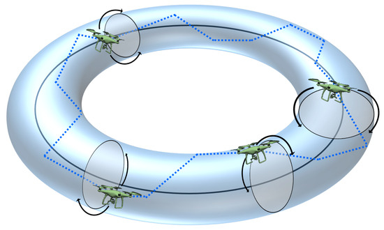
Figure 17. Outline of the surveillance path with chaotic maneuvering.

To perform a maneuver, any of the chaotic maps proposed in the previous section can be used. So each time a maneuver must be performed, the value of the chaotic map $x_i$ is mapped in the angle interval $\varphi \in [-90,90]$. This angle value corresponds to the amount of clockwise or counter-clockwise rotation that the agent will perform around on the circular area, defined from the frame of motion of the agent, intersecting the torus it moves on. The angle of rotation is limited to half the circular area to reduce redundant maneuvering, and it is motivated by [38], where a similar limitation is imposed to the turning of the agent. A schematic of this is shown in Figure 18. The advantage of using the proposed maps is that for longer simulations, it is possible to switch between parameter pairs $(a,b)$ so that the chaotic time series changes its statistical behavior over time, leading to an even more unpredictable trajectory.

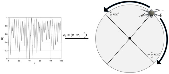
Figure 18. Frame of reference for the UAV agent. The map’s values are mapped into angles in the unit circle.

This process repeats any time a maneuver is set to be performed, and can be repeated for any number of times that the agent will perform a full crossing along the path of interest. The outline of this process is given in the Algorithm 1 below.

Algorithm 1: Chaotic Maneuvering Algorithm.

Input.  A closed surveillance path of interest. A toroidal surface around the closed path. A starting position on the torus, for the autonomous agent. A choice of N, denoting the amount of maneuverings performed as the agent moves along the torus. A chosen chaotic map from the above, with set parameters $a,b,c$ and initial condition $w_0$. Loop  For $i=1:N$. Step 1.  Compute $w_i$. Step 2.  Map the value of the chaotic map into an angle as $${\varphi }_i=180w_i-90.$$ (7) Step 3.  Rotate the agent along the circular frame of reference ${\varphi }_i$ angles as in Figure 18. End of loop.  If the traversing around the surveilled path needs to be repeated, then the loop is repeated.

4.3. Simulation Results

To showcase the proposed technique, a series of simulations are performed on a circular area of diameter 20 points, and a toroidal area of diameter 2 points around it. The points here may represent meters, or any other measure, depending on the size of the path considered. For this trajectory, a change of direction is performed at $N=100$ equally spaced intervals. The initial position of the agent is on $(X,Y,Z)=(9,0,10)$. For the chaotic maps used, $w_0=0.111$.

4.3.1. Periodic Motion

Initially, two examples are considered, where the motion is periodic. In Figure 19a, a scenario is shown, where in each iteration the agent rotates five degrees counter-clockwise. The motion here is smooth, but also very predictable. Figure 19b also shows the coordinates of the agent, as it progresses on the torus trajectory. Similarly, Figure 20a,b show a periodic motion, where in each iteration the agent rotates 15 degrees counter-clockwise. These two examples of periodic traversing can be considered a standardized approach to surveilling maneuvers. They are smooth but predictable.

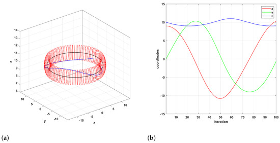
Figure 19. Periodic motion of the UAV agent, with a rotation of 5 degrees per iteration. (a) Trajectory of the UAV agent. (b) Coordinates of the UAV agent.

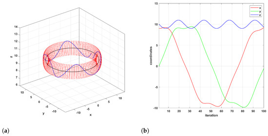
Figure 20. Periodic motion of the UAV agent, with a rotation of 15 degrees per iteration. (a) Trajectory of the UAV agent. (b) Coordinates of the UAV agent.

4.3.2. Chaotic Motion

To counter this predictability, we now consider a chaotic maneuvering. The first such example is shown in Figure 21a, where the tent map (3) is used with parameters $a=c=0$, $b=0.5001$. The trajectory now becomes much more erratic than before. This can be seen as well from the coordinate graph of Figure 21b. The degrees of rotation fed from the chaotic map in each iteration are shown in Figure 22, where it can be seen that there is a balanced amount of positive and negative rotation commands.

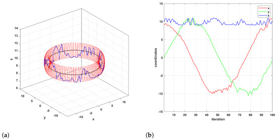
Figure 21. Chaotic motion of the UAV agent, using the map (3) for $a=0$, $b=0.5001$, and $c=0$. (a) Chaotic motion trajectory of the UAV agent. (b) Coordinates of the UAV agent.

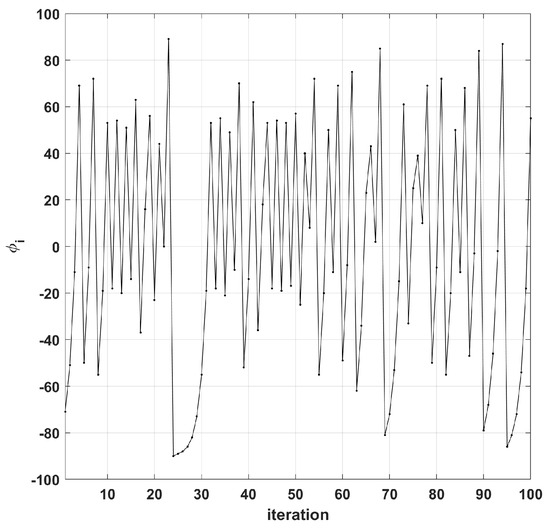
Figure 22. Rotation angles generated for the chaotic motion trajectory, using the map (3) for $a=0$, $b=0.5001$, and $c=0$.

As a second example, the same map is used, this time with parameters $a=0.4$, $b=0.8$, and $c=0$. The simulation result is shown in Figure 23a, and the coordinates of the agent are shown in Figure 23b. The motion is again unpredictable, with significant maneuvering. The chaotic degrees of rotation are shown in Figure 24, where it can be seen that there is an inclination towards positive rotations.

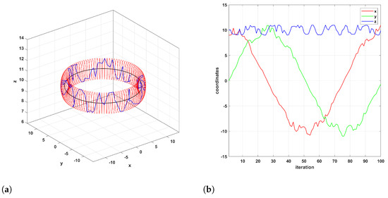
Figure 23. Chaotic motion of the UAV agent, using the map (3) for $a=0.4$, $b=0.8$, and $c=0$. (a) Chaotic motion trajectory of the UAV agent. (b) Coordinates of the UAV agent.

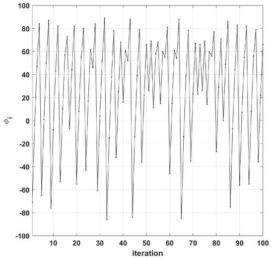
Figure 24. Rotation angles generated for the chaotic motion trajectory, using the map (3) for $a=0.4$, $b=0.8$, and $c=0$.

This was expected, as from the diagrams of Figure 1 and Figure 3b, we know that the tent map becomes right-skewed for higher values of $a,b$. Still, this does not affect the unpredictability of the motion. More importantly, this skewness can be of advantage to the trajectory design, when the parameter pairs vary over time.

Finally, an example of two consecutive rotations is considered, shown in Figure 25a,b and Figure 26. In Figure 25, the first rotation is shown in blue, and the second in green. Clearly, due to the inherent sensitivity of the chaotic map, the two trajectories are unrelated to each other; thus, knowledge of the first rotation points will in no way yield information about the possible future transitions performed during the second rotation.

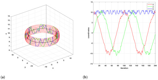
Figure 25. Chaotic motion trajectory of the UAV agent, using the map (3) for $a=0.4$, $b=0.8$, and $c=0$, when performing two loops around the set trajectory. (a) Chaotic motion trajectory of the UAV agent. (b) Coordinates of the UAV agent.

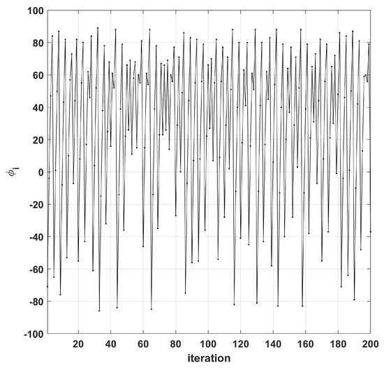
Figure 26. Rotation angles generated for the chaotic motion trajectory, using the map (3) for $a=0.4$, $b=0.8$ and $c=0$, when performing two loops around the set trajectory.

Overall, it is clear that the use of the chaotic maps proposed can easily be adopted as computationally light sources of randomness to introduce unpredictability in the motion of an agent traversing through a predefined path. Of course, what must be noted here is that in the simulations above, the dynamics of a UAV agent were not taken into account, but rather, a series of chaotic trajectory positions around a torus were generated. These can then be followed by a UAV agent by applying appropriate control techniques. So the technique proposed here is a general architecture, which can be further adopted by specialists when considering specific UAV dynamics and limitations. For example, the amount of rotation in each iteration can be reduced from $[-90,90]$ degrees to a smaller interval, depending on the efficiency of the agent.

5. Conclusions

This work considered a family of piecewise chaotic maps. The maps consist of three control parameters that are used to interpolate the endpoints of each subfunction at the desired positions in order to tune the distribution of the resulting time series. By considering five different chaotic maps from this family, it was deduced that it is possible to affect the statistical mean of the map’s chaotic time series, by changing the control parameters, in order to affect the domain and mapping interval of each subfunction. This capability can be of use in many chaos-based applications, like optimization, secure communications, and surveillance. For that matter, the application of chaotic surveillance was considered, by proposing a strategy for maneuvering a UAV chaotically on a toroidal area around a predefined trajectory.

There are several research topics that can extend the results of the current work. Although this work considered a numerical approach for the tuning of the statistical behavior of the map based on the geometric properties of each subfunction, it is of interest to derive a theoretical proof for the effect of parameters $a,b$ to the statistical properties of the map. Moreover, another interesting topic is to evaluate the use of the proposed maps in chaos-based optimization algorithms. It would also be interesting to study the use of the proposed maps in chaos-based communications for hiding an information signal and transmitting it through a public channel.

In addition to the above, there have been recent developments for two families of piecewise chaotic maps. The first family is that of maps composed of functions based on fuzzy numbers [44,45]. The other family of piecewise maps is that of no equilibria maps [46,47]. It would thus be of interest to study the aforementioned families of maps, with respect to the ability to tune their statistical characteristics.

Finally, it is of interest to develop an experimental realization of the proposed chaotic trajectory using a UAV in a real environment. For the aforementioned topics, there are some undergoing studies from our research group.

References

- Kaddoum, G. Wireless chaos-based communication systems: A comprehensive survey. IEEE Access 2016, 4, 2621–2648. [Google Scholar] [CrossRef]
- Tutueva, A.V.; Nepomuceno, E.G.; Karimov, A.I.; Andreev, V.S.; Butusov, D.N. Adaptive chaotic maps and their application to pseudo-random numbers generation. Chaos Solitons Fractals 2020, 133, 109615. [Google Scholar] [CrossRef]
- Wang, Y.; Liu, Z.; Ma, J.; He, H. A pseudorandom number generator based on piecewise logistic map. Nonlinear Dyn. 2016, 83, 2373–2391. [Google Scholar] [CrossRef]
- Irfan, M.; Ali, A.; Khan, M.A.; Ehatisham-ul Haq, M.; Mehmood Shah, S.N.; Saboor, A.; Ahmad, W. Pseudorandom number generator (prng) design using hyper-chaotic modified robust logistic map (hc-mrlm). Electronics 2020, 9, 104. [Google Scholar] [CrossRef]
- Lambić, D. Security analysis and improvement of the pseudo-random number generator based on piecewise logistic map. J. Electron. Test. 2019, 35, 519–527. [Google Scholar] [CrossRef]
- Liu, W.; Sun, K.; He, S.; Wang, H. The Parallel Chaotification Map and Its Application. IEEE Trans. Circuits Syst. I Regul. Pap. 2023, 70, 3689–3698. [Google Scholar] [CrossRef]
- Özkaynak, F. Brief review on application of nonlinear dynamics in image encryption. Nonlinear Dyn. 2018, 92, 305–313. [Google Scholar] [CrossRef]
- Zolfaghari, B.; Koshiba, T. Chaotic image encryption: State-of-the-art, ecosystem, and future roadmap. Appl. Syst. Innov. 2022, 5, 57. [Google Scholar] [CrossRef]
- Cetina-Denis, J.J.; Lopéz-Gutiérrez, R.M.; Cruz-Hernández, C.; Arellano-Delgado, A. Design of a Chaotic Trajectory Generator Algorithm for Mobile Robots. Appl. Sci. 2022, 12, 2587. [Google Scholar] [CrossRef]
- Gohari, P.S.; Mohammadi, H.; Taghvaei, S. Using chaotic maps for 3D boundary surveillance by quadrotor robot. Appl. Soft Comput. 2019, 76, 68–77. [Google Scholar] [CrossRef]
- Curiac, D.I.; Banias, O.; Volosencu, C.; Curiac, C.D. Novel bioinspired approach based on chaotic dynamics for robot patrolling missions with adversaries. Entropy 2018, 20, 378. [Google Scholar] [CrossRef] [PubMed]
- Saremi, S.; Mirjalili, S.; Lewis, A. Biogeography-based optimisation with chaos. Neural Comput. Appl. 2014, 25, 1077–1097. [Google Scholar] [CrossRef]
- Yang, D.; Liu, Z.; Zhou, J. Chaos optimization algorithms based on chaotic maps with different probability distribution and search speed for global optimization. Commun. Nonlinear Sci. Numer. Simul. 2014, 19, 1229–1246. [Google Scholar] [CrossRef]
- Tawhid, M.A.; Ibrahim, A.M. Improved salp swarm algorithm combined with chaos. Math. Comput. Simul. 2022, 202, 113–148. [Google Scholar] [CrossRef]
- Saxena, A.; Kumar, R.; Das, S. β-chaotic map enabled grey wolf optimizer. Appl. Soft Comput. 2019, 75, 84–105. [Google Scholar] [CrossRef]
- Fiori, S.; Di Filippo, R. An improved chaotic optimization algorithm applied to a DC electrical motor modeling. Entropy 2017, 19, 665. [Google Scholar] [CrossRef]
- Grassi, G. Chaos in the Real World: Recent Applications to Communications, Computing, Distributed Sensing, Robotic Motion, Bio-Impedance Modelling and Encryption Systems. Symmetry 2021, 13, 2151. [Google Scholar] [CrossRef]
- Zang, H.; Yuan, Y.; Wei, X. Research on Pseudorandom Number Generator Based on Several New Types of Piecewise Chaotic Maps. Math. Probl. Eng. 2021, 2021, 1375346. [Google Scholar] [CrossRef]
- Zhang, Z.; Wang, Y.; Zhang, L.Y.; Zhu, H. A novel chaotic map constructed by geometric operations and its application. Nonlinear Dyn. 2020, 102, 2843–2858. [Google Scholar] [CrossRef]
- Nagaraj, N. The Unreasonable Effectiveness of the Chaotic Tent Map in Engineering Applications. Chaos Theory Appl. 2022, 4, 197–204. [Google Scholar] [CrossRef]
- Chaves, D.P.; Souza, C.E.; Pimentel, C. A smooth chaotic map with parameterized shape and symmetry. EURASIP J. Adv. Signal Process. 2016, 2016, 122. [Google Scholar] [CrossRef]
- Zhang, S.; Liu, L. A novel image encryption algorithm based on SPWLCM and DNA coding. Math. Comput. Simul. 2021, 190, 723–744. [Google Scholar] [CrossRef]
- Zhao, X.; Zang, H.; Wei, X. Construction of a novel n th-order polynomial chaotic map and its application in the pseudorandom number generator. Nonlinear Dyn. 2022, 110, 821–839. [Google Scholar] [CrossRef]
- Berliner, L.M. Statistics, probability and chaos. Stat. Sci. 1992, 7, 69–90. [Google Scholar] [CrossRef]
- Barbosa, W.A.; Rosero, E.J.; Tredicce, J.R.; Leite, J.R.R. Statistics of chaos in a bursting laser. Phys. Rev. A 2019, 99, 053828. [Google Scholar] [CrossRef]
- Hilliam, R.M.; Lawrance, A.J. The dynamics and statistics of bivariate chaotic maps in communications modeling. Int. J. Bifurc. Chaos 2004, 14, 1177–1194. [Google Scholar] [CrossRef]
- Cicek, I.; Pusane, A.E.; Dundar, G. A novel design method for discrete time chaos based true random number generators. Integration 2014, 47, 38–47. [Google Scholar] [CrossRef]
- Boyarsky, A.; Góra, P. Laws of Chaos: Invariant Measures and Dynamical Systems in One Dimension; Birkhäuser Boston: Boston, MA, USA, 1997. [Google Scholar]
- McDonald, A.M.; van Wyk, M.A.; Chen, G. The inverse Frobenius-Perron problem: A survey of solutions to the original problem formulation. AIMS Math. 2021, 6, 11200–11232. [Google Scholar] [CrossRef]
- Lai, D.; Chen, G. Generating different statistical distributions by the chaotic skew tent map. Int. J. Bifurc. Chaos Appl. Sci. Eng. 2000, 10, 1509–1512. [Google Scholar] [CrossRef]
- Lawnik, M. Generation of pseudo-random numbers from given probabilistic distribution with the use of chaotic maps. AIP Conf. Proc. 2018, 1926, 020025. [Google Scholar] [CrossRef]
- Nie, X.; Coca, D.; Luo, J.; Birkin, M. Solving the inverse Frobenius-Perron problem using stationary densities of dynamical systems with input perturbations. Commun. Nonlinear Sci. Numer. Simul. 2020, 90, 105302. [Google Scholar] [CrossRef]
- Koga, S. The Inverse Problem of Flobenius-Perron Equations in 1D Difference Systems: 1D Map Idealization. Prog. Theor. Phys. 1991, 86, 991–1002. [Google Scholar] [CrossRef]
- Fox, C.; Hsiao, L.J.; Lee, J.E.K. Solutions of the Multivariate Inverse Frobenius–Perron Problem. Entropy 2021, 23, 838. [Google Scholar] [CrossRef] [PubMed]
- Moysis, L.; Lawnik, M.; Baptista, M.S.; Goudos, S.; Volos, C. Construction of Piecewise Chaotic Maps with Tunable Statistical Mean. In Proceedings of the 2023 12th International Conference on Modern Circuits and Systems Technologies (MOCAST), IEEE, Athens, Greece, 28–30 June 2023; pp. 1–4. [Google Scholar]
- Sridharan, K.; Ahmadabadi, Z.N. A multi-system chaotic path planner for fast and unpredictable online coverage of terrains. IEEE Robot. Autom. Lett. 2020, 5, 5268–5275. [Google Scholar] [CrossRef]
- Curiac, D.I.; Volosencu, C. A 2D chaotic path planning for mobile robots accomplishing boundary surveillance missions in adversarial conditions. Commun. Nonlinear Sci. Numer. Simul. 2014, 19, 3617–3627. [Google Scholar] [CrossRef]
- Artemiou, P.; Moysis, L.; Kafetzis, I.; Bardis, N.G.; Lawnik, M.; Volos, C. Chaotic Agent Navigation: Achieving Uniform Exploration Through Area Segmentation. In Proceedings of the 2022 12th International Conference on Dependable Systems, Services and Technologies (DESSERT), IEEE, Athens, Greece, 9–11 December 2022; pp. 1–7. [Google Scholar]
- Curiac, D.I.; Volosencu, C. Path planning algorithm based on Arnold cat map for surveillance UAVs. Def. Sci. J. 2015, 65, 483–488. [Google Scholar] [CrossRef]
- Li, C.; Song, Y.; Wang, F.; Liang, Z.; Zhu, B. Chaotic path planner of autonomous mobile robots based on the standard map for surveillance missions. Math. Probl. Eng. 2015, 2015, 263964. [Google Scholar] [CrossRef]
- Curiac, D.I.; Volosencu, C. Imparting protean behavior to mobile robots accomplishing patrolling tasks in the presence of adversaries. Bioinspir. Biomim. 2015, 10, 056017. [Google Scholar] [CrossRef]
- Curiac, D.I.; Volosencu, C. Chaotic trajectory design for monitoring an arbitrary number of specified locations using points of interest. Math. Probl. Eng. 2012, 2012, 940276. [Google Scholar] [CrossRef]
- Kafetzis, I.; Moysis, L.; Volos, C.; Stouboulos, I.; Valavanis, K. Area surveillance using a uav with mounted chaotic camera. In Proceedings of the 2021 International Conference on Unmanned Aircraft Systems (ICUAS), IEEE, Athens, Greece, 15–18 June 2021; pp. 53–62. [Google Scholar]
- Akraam, M.; Rashid, T.; Zafar, S. An image encryption scheme proposed by modifying chaotic tent map using fuzzy numbers. Multimed. Tools Appl. 2023, 82, 16861–16879. [Google Scholar] [CrossRef]
- Moysis, L.; Volos, C.; Jafari, S.; Munoz-Pacheco, J.M.; Kengne, J.; Rajagopal, K.; Stouboulos, I. Modification of the logistic map using fuzzy numbers with application to pseudorandom number generation and image encryption. Entropy 2020, 22, 474. [Google Scholar] [CrossRef] [PubMed]
- Jafari, S.; Pham, V.T.; Golpayegani, S.M.R.H.; Moghtadaei, M.; Kingni, S.T. The relationship between chaotic maps and some chaotic systems with hidden attractors. Int. J. Bifurc. Chaos 2016, 26, 1650211. [Google Scholar] [CrossRef]
- García-Grimaldo, C.; Campos-Cantón, E. Exploring a family of Bernoulli-like shift chaotic maps and its amplitude control. Chaos Solitons Fractals 2023, 175, 113951. [Google Scholar] [CrossRef]
Disclaimer/Publisher’s Note: The statements, opinions and data contained in all publications are solely those of the individual author(s) and contributor(s) and not of MDPI and/or the editor(s). MDPI and/or the editor(s) disclaim responsibility for any injury to people or property resulting from any ideas, methods, instructions or products referred to in the content. |
© 2023 by the authors. Licensee MDPI, Basel, Switzerland. This article is an open access article distributed under the terms and conditions of the Creative Commons Attribution (CC BY) license (https://creativecommons.org/licenses/by/4.0/).