
The Proxy-SU(3) Symmetry in Atomic Nuclei

 ,
,  and
and
Abstract
1. Introduction
2. SU(3) Symmetry in Nuclear Structure
3. Nucleon Pairs Favoring Deformation
4. The Proxy-SU(3) Approximation
5. Corroboration of Proxy-SU(3) through Nilsson Model Calculations
6. Proxy-SU(3) Symmetry in the Spherical Shell Model Basis
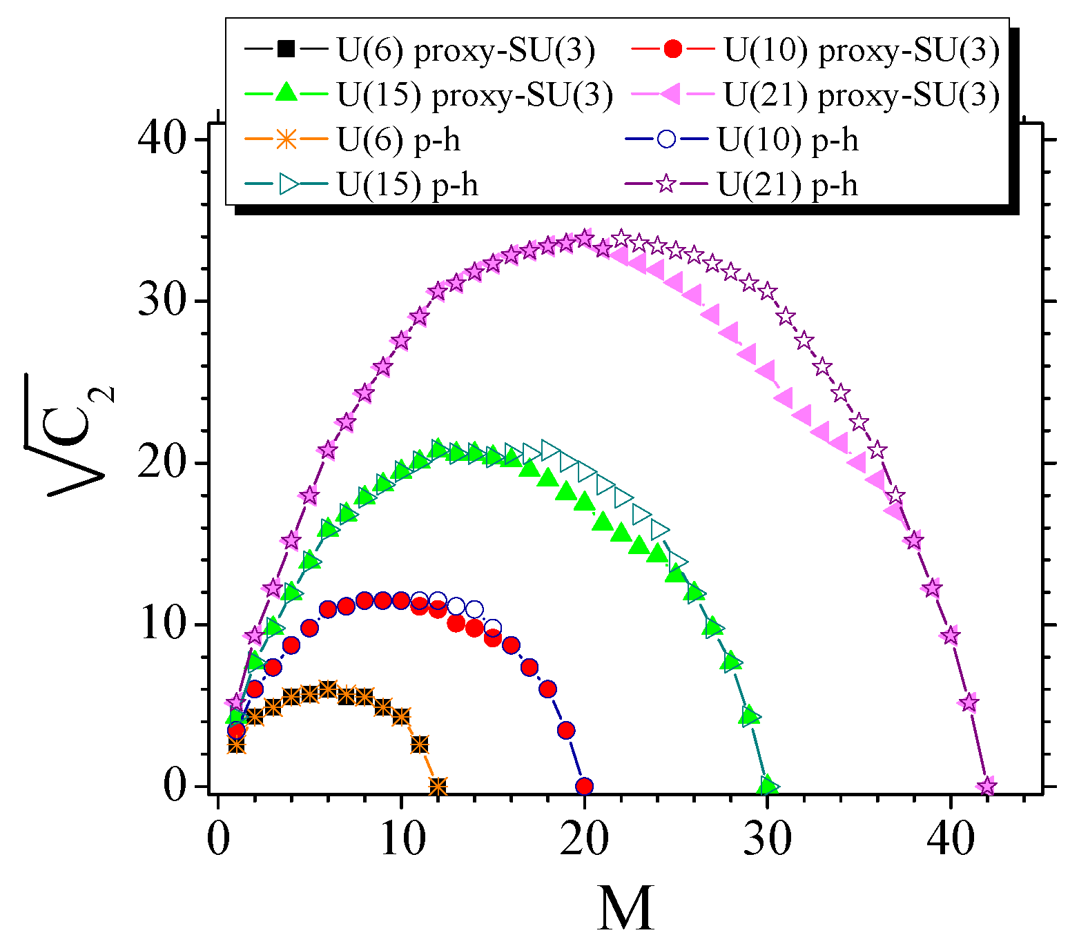
7. The Dominance of the Highest Weight Irreducible Representations of SU(3)
8. Physical Consequences of the Dominance of the Highest Weight Irreps
8.1. Prolate over Oblate Dominance

| 8–20 | 8–20 | 28–50 | 28–50 | 50–82 | 50–82 | 82–126 | 82–126 | 126–184 | 184–258 | ||
|---|---|---|---|---|---|---|---|---|---|---|---|
| sd | sd | pf | pf | sdg | sdg | PFH | PFH | sdgi | PFHj | ||
| M | irrep | U(6) | U(6) | U(10) | U(10) | U(15) | U(15) | U(21) | U(21) | U(28) | U(36) |
| hw | C | hw | C | hw | C | hw | C | hw | hw | ||
| 0 | (0,0) | (0,0) | (0,0) | (0,0) | (0,0) | (0,0) | (0,0) | (0,0) | (0,0) | (0,0) | |
| 1 | [1] | (2,0) | (2,0) | (3,0) | (3,0) | (4,0) | (4,0) | (5,0) | (5,0) | (6,0) | (7,0) |
| 2 | [2] | (4,0) | (4,0) | (6,0) | (6,0) | (8,0) | (8,0) | (10,0) | (10,0) | (12,0) | (14,0) |
| 3 | [21] | (4,1) | (4,1) | (7,1) | (7,1) | (10,1) | (10,1) | (13,1) | (13,1) | (16,1) | (19,1) |
| 4 | [] | (4,2) | (4,2) | (8,2) | (8,2) | (12,2) | (12,2) | (16,2) | (16,2) | (20,2) | (24,2) |
| 5 | [1] | (5,1) | (5,1) | (10,1) | (10,1) | (15,1) | (15,1) | (20,1) | (20,1) | (25,1) | (30,1) |
| 6 | [] | (6,0) | (0,6) | (12,0) | (12,0) | (18,0) | (18,0) | (24,0) | (24,0) | (30,0) | (36,0) |
| 7 | [1] | (4,2) | (1,5) | (11,2) | (11,2) | (18,2) | (18,2) | (25,2) | (25,2) | (32,2) | (39,2) |
| 8 | [] | (2,4) | (2,4) | (10,4) | (10,4) | (18,4) | (18,4) | (26,4) | (26,4) | (34,4) | (42,4) |
| 9 | [1] | (1,4) | (1,4) | (10,4) | (10,4) | (19,4) | (19,4) | (28,4) | (28,4) | (37,4) | (46,4) |
| 10 | [] | (0,4) | (0,4) | (10,4) | (4,10) | (20,4) | (20,4) | (30,4) | (30,4) | (40,4) | (50,4) |
| 11 | [1] | (0,2) | (0,2) | (11,2) | (4,10) | (22,2) | (22,2) | (33,2) | (33,2) | (44,2) | (55,2) |
| 12 | [] | (0,0) | (0,0) | (12,0) | (4,10) | (24,0) | (24,0) | (36,0) | (36,0) | (48,0) | (60,0) |
| 13 | [1] | (9,3) | (2,11) | (22,3) | (22,3) | (35,3) | (35,3) | (48,3) | (61,3) | ||
| 14 | [] | (6,6) | (0,12) | (20,6) | (20,6) | (34,6) | (34,6) | (48,6) | (62,6) | ||
| 15 | [1] | (4,7) | (1,10) | (19,7) | (7,19) | (34,7) | (34,7) | (49,7) | (64,7) | ||
| 16 | [] | (2,8) | (2,8) | (18,8) | (6,20) | (34,8) | (34,8) | (50,8) | (66,8) | ||
| 17 | [1] | (1,7) | (1,7) | (18,7) | (3,22) | (35,7) | (35,7) | (52,7) | (69,7) | ||
| 18 | [] | (0,6) | (0,6) | (18,6) | (0,24) | (36,6) | (36,6) | (54,6) | (72,6) | ||
| 19 | [1] | (0,3) | (0,3) | (19,3) | (2,22) | (38,3) | (38,3) | (57,3) | (76,3) | ||
| 20 | [] | (0,0) | (0,0) | (20,0) | (4,20) | (40,0) | (40,0) | (60,0) | (80,0) | ||
| 21 | [1] | (16,4) | (4,19) | (37,4) | (4,37) | (58,4) | (79,4) | ||||
| 22 | [] | (12,8) | (4,18) | (34,8) | (0,40) | (56,8) | (78,8) | ||||
| 23 | [1] | (9,10) | (2,18) | (32,10) | (3,38) | (55,10) | (78,10) | ||||
| 24 | [] | (6,12) | (0,18) | (30,12) | (6,36) | (54,12) | (78,12) | ||||
| 25 | [1] | (4,12) | (1,15) | (29,12) | (7,35) | (54,12) | (79,12) | ||||
| 26 | [] | (2,12) | (2,12) | (28,12) | (8,34) | (54,12) | (80,12) | ||||
| 27 | [1] | (1,10) | (1,10) | (28,10) | (7,34) | (55,10) | (82,10) | ||||
| 28 | [] | (0.8) | (0,8) | (28,8) | (6,34) | (56,8) | (84,8) | ||||
| 29 | [1] | (0,4) | (0,4) | (29,4) | (3,35) | (58,4) | (87,4) | ||||
| 30 | [] | (0,0) | (0,0) | (30,0) | (0,36) | (60,0) | (90,0) | ||||
| 31 | [1] | (25,5) | (2,33) | (56,5) | (87,5) | ||||||
| 32 | [] | (20,10) | (4,30) | (52,10) | (84,10) | ||||||
| 33 | [1] | (16,13) | (4,28) | (49,13) | (82,13) | ||||||
| 34 | [] | (12,16) | (4,26) | (46,16) | (80,16) | ||||||
| 35 | [1] | (9,17) | (2,25) | (44,17) | (79,17) | ||||||
| 36 | [] | (6,18) | (0,24) | (42,18) | (78,18) | ||||||
| 37 | [1] | (4,17) | (1,20) | (41,17) | (78,17) | ||||||
| 38 | [] | (2,16) | (2,16) | (40,16) | (78,16) | ||||||
| 39 | [1] | (1,13) | (1,13) | (40,13) | (79,13) | ||||||
| 40 | [] | (0,10) | (0,10) | (40,10) | (80,10) | ||||||
| 41 | [1] | (0,5) | (0,5) | (41,5) | (82,5) | ||||||
| 42 | [] | (0,0) | (0,0) | (42,0) | (84,0) | ||||||
| 43 | [1] | (36,6) | (79,6) | ||||||||
| 44 | [] | (30,12) | (74,12) | ||||||||
| 45 | [1] | (25,16) | (70,16) | ||||||||
| 46 | [] | (20,20) | (66,20) | ||||||||
| 47 | [1] | (16,22) | (63,22) | ||||||||
| 48 | [] | (12,24) | (60,24) | ||||||||
| 49 | [1] | (9,24) | (58,24) | ||||||||
| 50 | [] | (6,24) | (56,24) | ||||||||
| 51 | [1] | (4,22) | (55,22) | ||||||||
| 52 | [] | (2,20) | (54,20) | ||||||||
| 53 | [1] | (1,16) | (54,16) | ||||||||
| 54 | [] | (0,12) | (54,12) | ||||||||
| 55 | [1] | (0,6) | (55,6) | ||||||||
| 56 | [] | (0,0) | (56,0) |
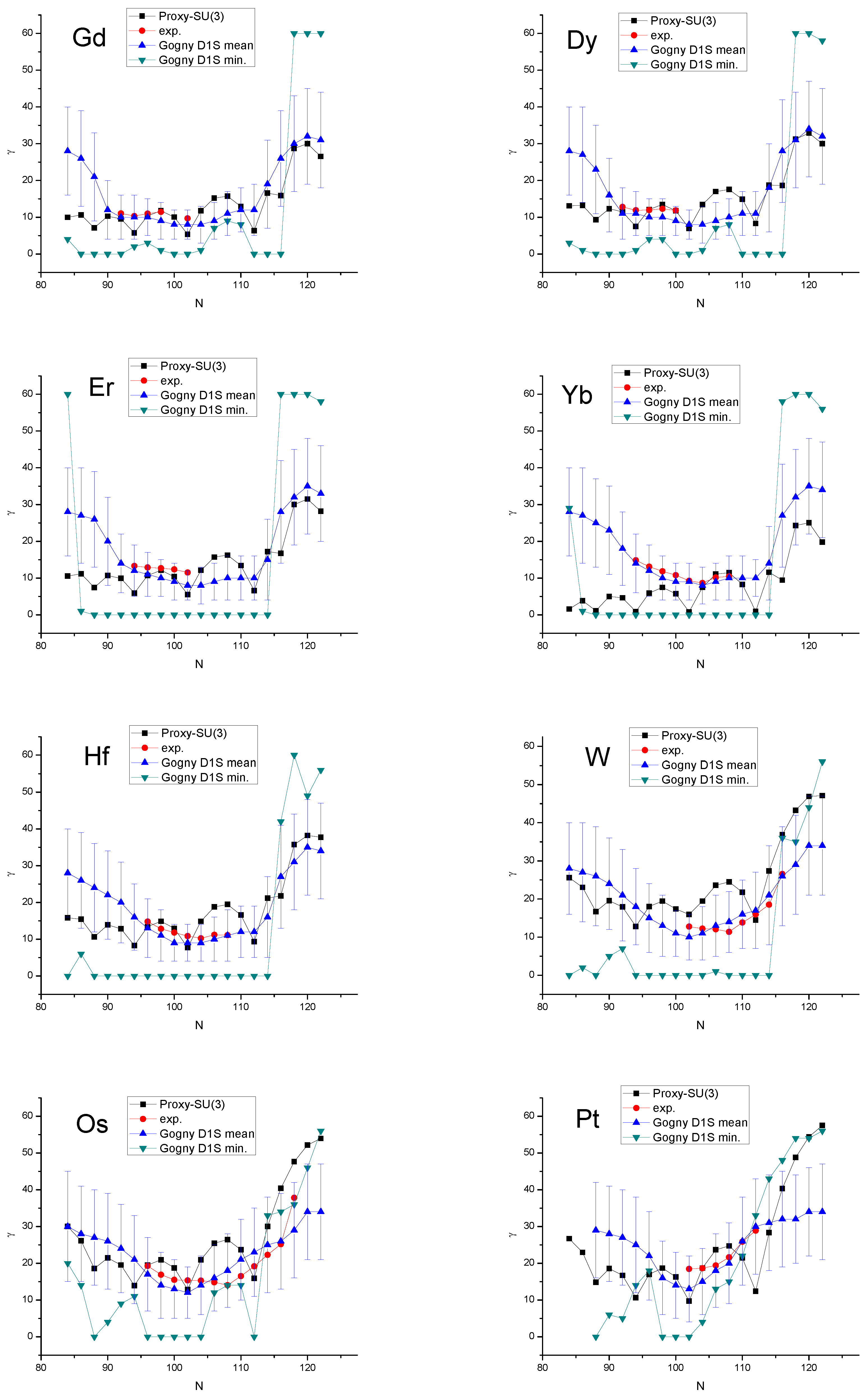
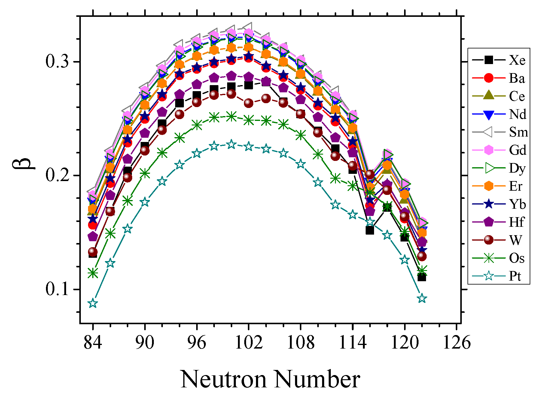
8.2. Parameter-Free Predictions for the Collective Variables and
8.3. Prolate to Oblate Shape/Phase Transition
9. Islands of Shape Coexistence
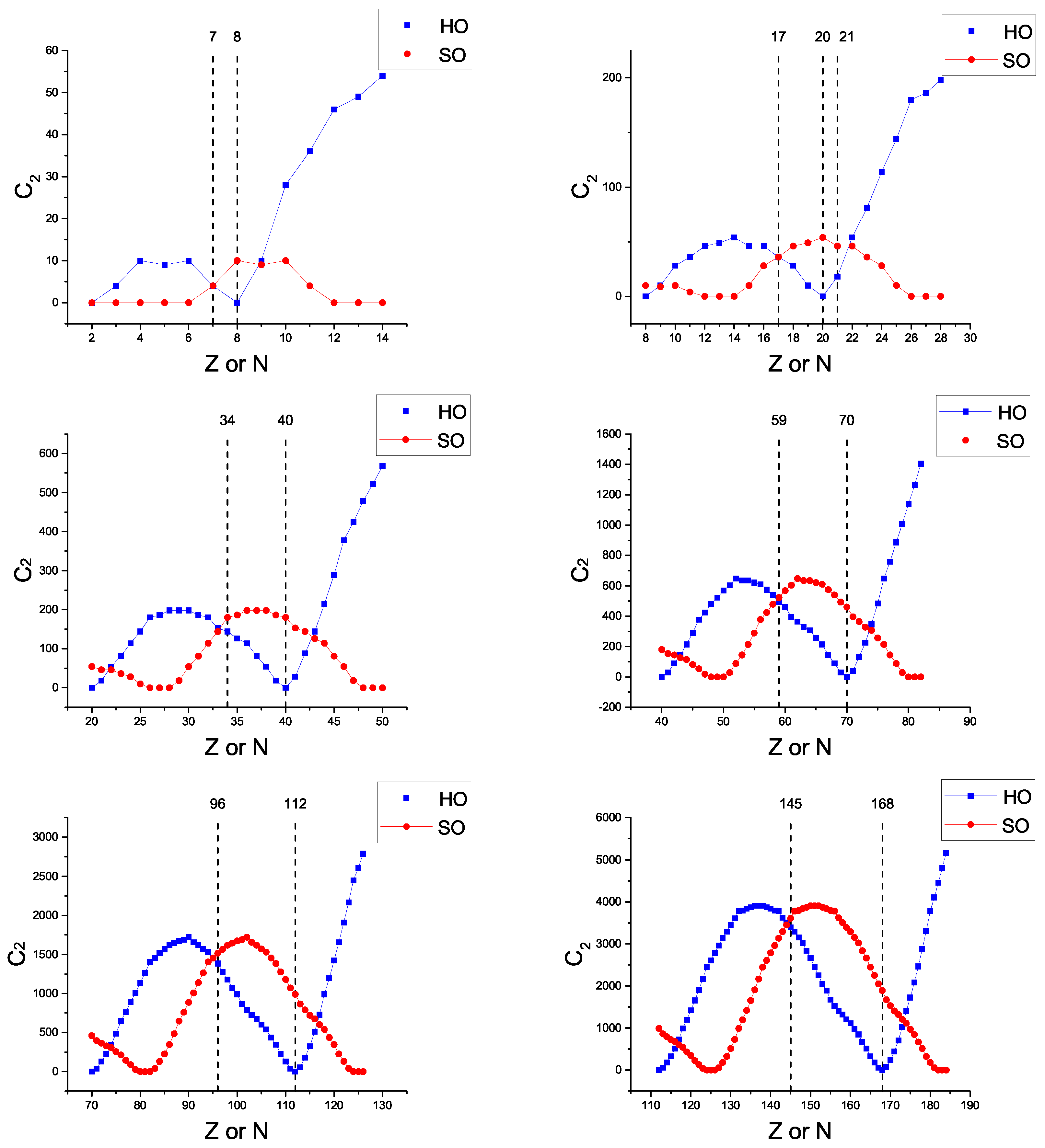
9.1. Harmonic Oscillator (HO) and Spin–Orbit (SO) Magic Numbers
9.2. A Dual Shell Mechanism for Shape Coexistence
9.3. From Stripes to Islands of Shape Coexistence
9.4. Multiple-Shape Coexistence
10. Conclusions and Outlook
Author Contributions
Funding
Institutional Review Board Statement
Informed Consent Statement
Data Availability Statement
Conflicts of Interest
References
- Wigner, E. On the consequences of the symmetry of the nuclear Hamiltonian on the spectroscopy of nuclei. Phys. Rev. 1937, 51, 106. [Google Scholar] [CrossRef]
- Franzini, P.; Radicati, L.A. On the validity of the supermultiplet model. Phys. Lett. 1963, 6, 322. [Google Scholar] [CrossRef]
- Hecht, K.T.; Pang, S.C. On the Wigner supermultiplet scheme. J. Math. Phys. 1969, 10, 1571. [Google Scholar] [CrossRef]
- Mayer, M.G. On closed shells in nuclei. Phys. Rev. 1948, 74, 235. [Google Scholar] [CrossRef]
- Mayer, M.G. On closed shells in nuclei. II. Phys. Rev. 1949, 75, 1969. [Google Scholar] [CrossRef]
- Haxel, O.; Jensen, J.H.D.; Suess, H.E. On the “magic numbers” in nuclear structure. Phys. Rev. 1949, 75, 1766. [Google Scholar] [CrossRef]
- Mayer, M.G.; Jensen, J.H.D. Elementary Theory of Nuclear Shell Structure; Wiley: New York, NY, USA, 1955. [Google Scholar]
- Wybourne, B.G. Classical Groups for Physicists; Wiley: New York, NY, USA, 1974. [Google Scholar]
- Moshinsky, M.; Smirnov, Y.F. The Harmonic Oscillator in Modern Physics; Harwood: Amsterdam, The Netherlands, 1996. [Google Scholar]
- Iachello, F. Lie Algebras and Applications; Springer: Berlin/Heidelberg, Germany, 2006. [Google Scholar]
- Bonatsos, D.; Klein, A. Exact boson mappings for nuclear neutron (proton) shell-model algebras having SU(3) subalgebras. Ann. Phys. 1986, 169, 61. [Google Scholar] [CrossRef]
- Nobel Foundation. Nobel Lectures, Physics 1963–1970; Elsevier: Amsterdam, The Netherlands, 1972. [Google Scholar]
- Rainwater, J. Nuclear energy level argument for a spheroidal nuclear model. Phys. Rev. 1950, 79, 432. [Google Scholar] [CrossRef]
- Bohr, A. The coupling of nuclear surface oscillations to the motion of individual nucleons. Mat. Fys. Medd. K. Dan. Vidensk. Selsk. 1952, 26. Available online: http://www.xuantianlinyu.com.cn/Jabref/RefPdf/Bohr1952pp.pdf (accessed on 1 January 2022).
- Bohr, A.; Mottelson, B.R. Nuclear Structure Vol. II: Nuclear Deformations; Benjamin: New York, NY, USA, 1975. [Google Scholar]
- Nobel Foundation. Nobel Lectures, Physics 1971–1980; Lundqvist, S., Ed.; World Scientific: Singapore, 1992. [Google Scholar]
- Nilsson, S.G. Binding states of individual nucleons in strongly deformed nuclei. Mat. Fys. Medd. K. Dan. Vidensk. Selsk. 1955, 29. Available online: http://gymarkiv.sdu.dk/MFM/kdvs/mfm%2020-29/MFM%2029-16.pdf (accessed on 1 January 2022).
- Ragnarsson, I.; Nilsson, S.G.; Sheline, R.K. Shell structure in nuclei. Phys. Rep. 1978, 45, 1. [Google Scholar] [CrossRef]
- Nilsson, S.G.; Ragnarsson, I. Shapes and Shells in Nuclear Structure; Cambridge University Press: Cambridge, UK, 1995. [Google Scholar]
- Takahashi, Y. SU(3) shell model in a deformed harmonic oscillator basis. Prog. Theor. Phys. 1975, 53, 461. [Google Scholar] [CrossRef][Green Version]
- Asherova, R.M.; Smirnov, Y.F.; Tolstoy, V.N.; Shustov, A.P. Algebraic approach to the projected deformed oscillator model. Nucl. Phys. A 1981, 355, 25. [Google Scholar] [CrossRef]
- Rosensteel, G.; Draayer, J.P. Symmetry algebra of the anisotropic harmonic oscillator with commensurate frequencies. J. Phys. A Math. Gen. 1989, 22, 1323. [Google Scholar] [CrossRef]
- Nazarewicz, W.; Dobaczewski, J. Dynamical symmetries, multiclustering, and octupole susceptibility in superdeformed and hyperdeformed nuclei. Phys. Rev. Lett. 1992, 68, 154. [Google Scholar] [CrossRef] [PubMed]
- Nazarewicz, W.; Dobaczewski, J.; Isacker, P.V. Shell model calculations at superdeformed shapes. AIP Conf. Proc. 1992, 259, 30. [Google Scholar]
- Bonatsos, D.; Daskaloyannis, C.; Kolokotronis, P.; Lenis, D. The symmetry algebra of the N-dimensional anisotropic quantum harmonic oscillator with rational ratios of frequencies and the Nilsson model. arXiv 1994, arXiv:hep-th/9411218. [Google Scholar]
- Elliott, J.P. Collective motion in the nuclear shell model. I. Classification schemes for states of mixed configurations. Proc. R. Soc. Lond. Ser. A 1958, 245, 128. [Google Scholar]
- Elliott, J.P. Collective motion in the nuclear shell model. II. The introduction of intrinsic wave-functions. Proc. R. Soc. Lond. Ser. A 1958, 245, 562. [Google Scholar]
- Elliott, J.P.; Harvey, M. Collective motion in the nuclear shell model. III. The calculation of spectra. Proc. R. Soc. Lond. Ser. A 1963, 272, 557. [Google Scholar]
- Wilsdon, C.E. A Survey of the Nuclear s-d Shell Using the SU(3) Coupling Scheme. Ph.D. Thesis, University of Sussex, Brighton, UK, 1965. [Google Scholar]
- Elliott, J.P.; Wildson, C.E. Collective motion in the nuclear shell model. IV. Odd-mass nuclei in the sd shell. Proc. R. Soc. Lond. Ser. A 1968, 302, 509. [Google Scholar]
- Harvey, M. The nuclear SU3 model. Adv. Nucl. Phys. 1968, 1, 67. [Google Scholar]
- Cseh, J. Some new chapters of the long history of SU(3). EPJ Web Conf. 2018, 194, 05001. [Google Scholar] [CrossRef][Green Version]
- Raychev, P.P. On the broken Sp(3,3) symmetry and the spectra of deformed even–even nuclei. Compt. Rend. Acad. Bulg. Sci. 1972, 25, 1503. [Google Scholar]
- Afanas’ev, G.N.; Abramov, S.A.; Raychev, P.P. Realization of the physical basis for SU(3) and the probabilities of E2 transitions in the SU(3) formalism. Yad. Fiz. 1972, 16, 53, Erratum in Sov. J. Nucl. Phys. 1973, 16, 27. [Google Scholar]
- Raychev, P.P. Parametrization of B(E2) transitions in deformed even–even nuclei within the framework of the SU(3) scheme. Yad. Fiz. 1972, 16, 1171, Erratum in Sov. J. Nucl. Phys. 1973, 16, 643. [Google Scholar]
- Raychev, P.P.; Roussev, R.P. Energy levels and reduced E2-transition probabilities of deformed even–even nuclei in the SU(3) scheme. Yad. Fiz. 1978, 27, 1501, Erratum in Sov. J. Nucl. Phys. 1978, 27, 792. [Google Scholar]
- Minkov, N.; Drenska, S.B.; Raychev, P.P.; Roussev, R.P.; Bonatsos, D. Broken SU(3) symmetry in deformed even–even nuclei. Phys. Rev. C 1997, 55, 2345. [Google Scholar] [CrossRef]
- Minkov, N.; Drenska, S.B.; Raychev, P.P.; Roussev, R.P.; Bonatsos, D. Ground-γ band coupling in heavy deformed nuclei and SU(3) contraction limit. Phys. Rev. C 1999, 60, 034305. [Google Scholar] [CrossRef]
- Minkov, N.; Drenska, S.B.; Raychev, P.P.; Roussev, R.P.; Bonatsos, D. Ground-γ band mixing and odd-even staggering in heavy deformed nuclei. Phys. Rev. C 2000, 61, 064301. [Google Scholar] [CrossRef]
- Afanas’ev, G.N.; Raychev, P.P. Dynamical symmetry groups in nuclei. Fiz. Elem. Chast. At. Yadra 1972, 3, 436, Erratum in Sov. J. Nucl. Phys. 1972, 3, 229. [Google Scholar]
- Hecht, K.T.; Adler, A. Generalized seniority for favored J ≠ 0 pairs in mixed configurations. Nucl. Phys. A 1969, 137, 129. [Google Scholar] [CrossRef]
- Arima, A.; Harvey, M.; Shimizu, K. Pseudo LS coupling and pseudo SU3 coupling schemes. Phys. Lett. B 1969, 30, 517. [Google Scholar] [CrossRef]
- Raju, R.D.R.; Draayer, J.P.; Hecht, K.T. Search for a coupling scheme in heavy deformed nuclei: The pseudo SU(3) model. Nucl. Phys. A 1973, 202, 433. [Google Scholar] [CrossRef]
- Draayer, J.P.; Weeks, K.J.; Hecht, K.T. Strength of the Qπ·Qν interaction and the strong-coupled pseudo-SU(3) limit. Nucl. Phys. A 1982, 381, 1. [Google Scholar] [CrossRef]
- Draayer, J.P.; Weeks, K.J. Shell-model description of the low-energy structure of strongly deformed nuclei. Phys. Rev. Lett. 1983, 51, 1422. [Google Scholar] [CrossRef]
- Draayer, J.P.; Weeks, K.J. Towards a shell model description of the low-energy structure of deformed nuclei I. even–even systems. Ann. Phys. 1984, 156, 41. [Google Scholar] [CrossRef]
- Draayer, J.P. Fermion models. In Algebraic Approaches to Nuclear Structure; Casten, R.F., Ed.; Harwood: Chur, Switzerland, 1993; p. 423. [Google Scholar]
- Castaños, O.; Moshinsky, M.; Quesne, C. Transformations from U(3) to pseudo U(3) basis. In Group Theory and Special Symmetries in Nuclear Physics Ann Arbor, 1991; Draayer, J.P., Jänecke, J., Eds.; World Scientific: Singapope, 1992; p. 80. [Google Scholar]
- Castaños, O.; Moshinsky, M.; Quesne, C. Transformation to pseudo-SU(3) in heavy deformed nuclei. Phys. Lett. B 1992, 277, 238. [Google Scholar] [CrossRef]
- Castaños, O.; Velázquez, A.V.; Hess, P.O.; Hirsch, J.G. Transformation to pseudo-spin-symmetry of a deformed Nilsson hamiltonian. Phys. Lett. B 1994, 321, 303. [Google Scholar] [CrossRef]
- Ginocchio, J.N. Pseudospin as a relativistic symmetry. Phys. Rev. Lett. 1997, 78, 436. [Google Scholar] [CrossRef]
- Ginocchio, J.N. On the relativisitic origins of pseudo-spin symmetry in nuclei. J. Phys. G Nucl. Part. Phys. 1999, 25, 617. [Google Scholar] [CrossRef]
- Janssen, D.; Jolos, R.V.; Dönau, F. An algebraic treatment of the nuclear quadrupole degree of freedom. Nucl. Phys. A 1974, 224, 93. [Google Scholar] [CrossRef]
- Arima, A.; Iachello, F. Collective nuclear states as representations of a SU(6) group. Phys. Rev. Lett. 1975, 35, 1069. [Google Scholar] [CrossRef]
- Arima, A.; Iachello, F. Interacting boson model of collective states I. The vibrational limit. Ann. Phys. 1976, 99, 253. [Google Scholar] [CrossRef]
- Arima, A.; Iachello, F. Interacting boson model of collective nuclear states II. The rotational limit. Ann. Phys. 1978, 111, 201. [Google Scholar] [CrossRef]
- Arima, A.; Iachello, F. Interacting boson model of collective nuclear states IV. The O(6) limit. Ann. Phys. 1979, 123, 468. [Google Scholar] [CrossRef]
- Iachello, F.; Arima, A. The Interacting Boson Model; Cambridge University Press: Cambridge, UK, 1987. [Google Scholar]
- Iachello, F.; Isacker, P.V. The Interacting Boson-Fermion Model; Cambridge University Press: Cambridge, UK, 1991. [Google Scholar]
- Frank, A.; Isacker, P.V. Symmetry Methods in Molecules and Nuclei; S y G Editores: México, Mexico, 2005. [Google Scholar]
- Rosensteel, G.; Rowe, D.J. Nuclear Sp(3,R) Model. Phys. Rev. Lett. 1977, 38, 10. [Google Scholar] [CrossRef]
- Rosensteel, G.; Rowe, D.J. On the algebraic formulation of collective models III. The symplectic shell model of collective motion. Ann. Phys. 1980, 126, 343. [Google Scholar] [CrossRef]
- Park, P.; Carvalho, J.; Vassanji, M.; Rowe, D.J. The shell-model theory of nuclear rotational states. Nucl. Phys. A 1984, 414, 93. [Google Scholar] [CrossRef]
- Rowe, D.J. Microscopic theory of the nuclear collective model. Rep. Prog. Phys. 1985, 48, 1419. [Google Scholar] [CrossRef]
- Rowe, D.J.; Wood, J.L. Fundamentals of Nuclear Models: Foundational Models; World Scientific: Singapore, 2010. [Google Scholar]
- Wybourne, B.G. The representation space of the nuclear symplectic Sp(6,R) shell model. J. Phys. A Math. Gen. 1992, 25, 4389. [Google Scholar] [CrossRef]
- Escher, J.; Draayer, J.P. Fermion realization of the nuclear Sp(6,R) model. J. Math. Phys. 1998, 39, 5123. [Google Scholar] [CrossRef]
- Ganev, H.G. Shell-model representations of the proton–neutron symplectic model. Eur. Phys. J. A 2015, 51, 84. [Google Scholar] [CrossRef]
- Ganev, H.G. Microscopic shell-model description of transitional nuclei. Eur. Phys. J. A 2022, 58, 182. [Google Scholar] [CrossRef]
- Ganev, H.G. Microscopic shell-model description of strongly deformed nuclei: 158Gd. Int. J. Mod. Phys. E 2022, 31, 2250047. [Google Scholar] [CrossRef]
- Georgieva, A.; Raychev, P.; Roussev, R. Interacting two-vector-boson model of collective motions in nuclei. J. Phys. G Nucl. Phys. 1982, 8, 1377. [Google Scholar] [CrossRef]
- Georgieva, A.; Raychev, P.; Roussev, R. Rotational limit of the interacting two-vector boson model. J. Phys. G Nucl. Phys. 1983, 9, 521. [Google Scholar] [CrossRef]
- Wu, C.-L.; Feng, D.H.; Chen, X.-G.; Chen, J.-Q.; Guidry, M.W. Fermion dynamical symmetry model of nuclei: Basis, Hamiltonian, and symmetries. Phys. Rev. C 1987, 36, 1157. [Google Scholar] [CrossRef]
- Navrátil, P.; Vary, J.P.; Barrett, B.R. Properties of 12C in the ab initio nuclear shell model. Phys. Rev. Lett. 2000, 84, 5728. [Google Scholar] [CrossRef]
- Navrátil, P.; Vary, J.P.; Barrett, B.R. Large-basis ab initio no-core shell model and its application to 12C. Phys. Rev. C 2000, 62, 054311. [Google Scholar] [CrossRef]
- Dytrych, T.; Sviratcheva, K.D.; Bahri, C.; Draayer, J.P.; Vary, J.P. Evidence for symplectic symmetry in ab initio no-core shell model results for light nuclei. Phys. Rev. Lett. 2007, 98, 162503. [Google Scholar] [CrossRef] [PubMed]
- Dytrych, T.; Sviratcheva, K.D.; Bahri, C.; Draayer, J.P.; Vary, J.P. Dominant role of symplectic symmetry in ab initio no-core shell model results for light nuclei. Phys. Rev. C 2007, 76, 014315. [Google Scholar] [CrossRef]
- Dytrych, T.; Sviratcheva, K.D.; Draayer, J.P.; Bahri, C.; Vary, J.P. Ab initio symplectic no-core shell model. J. Phys. G Nucl. Part. Phys. 2008, 35, 123101. [Google Scholar] [CrossRef]
- Tobin, G.K.; Ferriss, M.C.; Launey, K.D.; Dytrych, T.; Draayer, J.P.; Dreyfuss, A.C.; Bahri, C. Symplectic no-core shell-model approach to intermediate-mass nuclei. Phys. Rev. C 2014, 89, 034312. [Google Scholar] [CrossRef]
- Dytrych, T.; Maris, P.; Launey, K.D.; Draayer, J.P.; Vary, J.P.; Langr, D.; Saule, E.; Caprio, M.A.; Catalyurek, U.; Sosonkina, M. Efficacy of the SU(3) scheme for ab initio large-scale calculations beyond the lightest nuclei. Comp. Phys. Commun. 2016, 207, 202. [Google Scholar] [CrossRef]
- Launey, K.D.; Draayer, J.P.; Dytrych, T.; Sun, G.-H.; Dong, S.-H. Approximate symmetries in atomic nuclei from a large-scale shell-model perspective. Int. J. Mod. Phys. E 2015, 24, 1530005. [Google Scholar] [CrossRef]
- Launey, K.D.; Dytrych, T.; Draayer, J.P. Symmetry-guided large-scale shell-model theory. Prog. Part. Nucl. Phys. 2016, 89, 101. [Google Scholar] [CrossRef]
- Dytrych, T.; Launey, K.D.; Draayer, J.P.; Rowe, D.J.; Wood, J.L.; Rosensteel, G.; Bahri, C.; Langr, D.; Baker, R.B. Physics of Nuclei: Key Role of an Emergent Symmetry. Phys. Rev. Lett. 2020, 124, 042501. [Google Scholar] [CrossRef]
- Launey, K.D.; Dytrych, T.; Sargsyan, G.H.; Baker, R.B.; Draayer, J.P. Emergent symplectic symmetry in atomic nuclei. Eur. Phys. J. Spec. Top. 2020, 229, 2429. [Google Scholar] [CrossRef]
- Launey, K.D.; Marcenne, A.; Dytrych, T. Nuclear dynamics and reactions in the ab initio symmetry-adapted framework. Annu. Rev. Nucl. Part. Sci. 2021, 71, 253. [Google Scholar] [CrossRef]
- Kota, V.K.B. SU(3) Symmetry in Atomic Nuclei; Springer: Singapore, 2020. [Google Scholar]
- Bonatsos, D.; Martinou, A.; Assimakis, I.E.; Peroulis, S.K.; Sarantopoulou, S.; Minkov, N. Connecting the proxy-SU(3) symmetry to the shell model. Eur. Phys. J. Web Conf. 2021, 252, 02004. [Google Scholar] [CrossRef]
- Bonatsos, D.; Assimakis, I.E.; Minkov, N.; Martinou, A.; Cakirli, R.B.; Casten, R.F.; Blaum, K. Proxy-SU(3) symmetry in heavy deformed nuclei. Phys. Rev. C 2017, 95, 064325. [Google Scholar] [CrossRef]
- Bonatsos, D.; Assimakis, I.E.; Minkov, N.; Martinou, A.; Sarantopoulou, S.; Cakirli, R.B.; Casten, R.F.; Blaum, K. Analytic predictions for nuclear shapes, prolate dominance, and the prolate-oblate shape transition in the proxy-SU(3) model. Phys. Rev. C 2017, 95, 064326. [Google Scholar] [CrossRef]
- Bonatsos, D. Prolate over oblate dominance in deformed nuclei as a consequence of the SU(3) symmetry and the Pauli principle. Eur. Phys. J. A 2017, 53, 148. [Google Scholar] [CrossRef]
- de Shalit, A.; Goldhaber, M. Mixed configurations in nuclei. Phys. Rev. 1953, 92, 1211. [Google Scholar] [CrossRef]
- Talmi, I. Effective interactions and coupling schemes in nuclei. Rev. Mod. Phys. 1962, 34, 704. [Google Scholar] [CrossRef]
- Talmi, I. Generalized seniority and structure of semi-magic nuclei. Nucl. Phys. A 1971, 172, 1. [Google Scholar] [CrossRef]
- Talmi, I. Coupling schemes in nuclei. Riv. Nuovo Cim. 1973, 3, 85. [Google Scholar] [CrossRef]
- Talmi, I. Simple Models of Complex Nuclei; Harwood: Chur, Switzerland, 1993. [Google Scholar]
- Federman, P.; Pittel, S. Towards a unified microscopic description of nuclear deformation. Phys. Lett. B 1977, 69, 385. [Google Scholar] [CrossRef]
- Federman, P.; Pittel, S. Hartree-Fock-Bogolyubov study of deformation in the Zr-Mo region. Phys. Lett. B 1978, 77, 29. [Google Scholar] [CrossRef]
- Federman, P.; Pittel, S. Unified shell-model description of nuclear deformation. Phys. Rev. C 1979, 20, 820. [Google Scholar] [CrossRef]
- Casten, R.F. Possible Unified interpretation of heavy nuclei. Phys. Rev. Lett. 1985, 54, 1991. [Google Scholar] [CrossRef] [PubMed]
- Casten, R.F. NpNn systematics in heavy nuclei. Nucl. Phys. A 1985, 443, 1. [Google Scholar] [CrossRef]
- Casten, R.F.; Brenner, D.S.; Haustein, P.E. Valence p-n interactions and the development of collectivity in heavy nuclei. Phys. Rev. Lett. 1987, 58, 658. [Google Scholar] [CrossRef] [PubMed]
- Casten, R.F. Nuclear Structure from a Simple Perspective; Oxford University Press: Oxford, UK, 2000. [Google Scholar]
- Zuker, A.P.; Retamosa, J.; Poves, A.; Caurier, E. Spherical shell model description of rotational motion. Phys. Rev. C 1995, 52, R1741. [Google Scholar] [CrossRef] [PubMed]
- Zuker, A.P.; Poves, A.; Nowacki, F.; Lenzi, S.M. Nilsson-SU(3) self-consistency in heavy n = Z nuclei. Phys. Rev. C 2015, 92, 024320. [Google Scholar] [CrossRef]
- Kaneko, K.; Shimizu, N.; Mizusaki, T.; Sun, Y. Quasi-SU(3) coupling of (1h11/2, 2f7/2) across the n = 82 shell gap: Enhanced E2 collectivity and shape evolution in Nd isotopes. Phys. Rev. C 2021, 103, L021301. [Google Scholar] [CrossRef]
- Cakirli, R.B.; Brenner, D.S.; Casten, R.F.; Millman, E.A. proton–neutron interactions and the new atomic masses. Phys. Rev. Lett. 2005, 94, 092501, Erratum in Phys. Rev. Lett. 2005, 95, 119903. [Google Scholar] [CrossRef]
- Cakirli, R.B.; Casten, R.F. Direct empirical correlation between proton–neutron interaction strengths and the growth of collectivity in nuclei. Phys. Rev. Lett. 2006, 96, 132501. [Google Scholar] [CrossRef]
- Brenner, D.S.; Cakirli, R.B.; Casten, R.F. Valence proton–neutron interactions throughout the mass surface. Phys. Rev. C 2006, 73, 034315. [Google Scholar] [CrossRef]
- Cakirli, R.B.; Casten, R.F.; Winkler, R.; Blaum, K.; Kowalska, M. Enhanced sensitivity of nuclear binding energies to collective structure. Phys. Rev. Lett. 2009, 102, 082501. [Google Scholar] [CrossRef] [PubMed]
- Cakirli, R.B.; Blaum, K.; Casten, R.F. Indication of a mini-valence Wigner-like energy in heavy nuclei. Phys. Rev. C 2010, 82, 061304. [Google Scholar] [CrossRef]
- Bonatsos, D.; Karampagia, S.; Cakirli, R.B.; Casten, R.F.; Blaum, K.; Susam, L.A. Emergent collectivity in nuclei and enhanced proton–neutron interactions. Phys. Rev. C 2013, 88, 054309. [Google Scholar] [CrossRef]
- Stoitsov, M.; Cakirli, R.B.; Casten, R.F.; Nazarewicz, W.; Satula, W. Empirical proton–neutron interactions and nuclear density functional theory: Global, regional, and local comparisons. Phys. Rev. Lett. 2007, 98, 132502. [Google Scholar] [CrossRef] [PubMed]
- Sieja, K. Single-particle and collective structures in neutron-rich Sr isotopes. Universe 2022, 8, 23. [Google Scholar] [CrossRef]
- Lederer, C.M.; Shirley, V.S. (Eds.) Table of Isotopes, 7th ed.; Wiley: New York, NY, USA, 1978. [Google Scholar]
- Ring, P.; Schuck, P. The Nuclear Many-Body Problem; Springer: Berlin/Heidelberg, Germany, 1980. [Google Scholar]
- Davies, K.T.R.; Krieger, S.J. Harmonic-oscillator transformation coefficients. Can. J. Phys. 1991, 69, 62. [Google Scholar] [CrossRef]
- Chasman, R.R.; Wahlborn, S. Transformation scheme for harmonic-oscillator wave functions. Nucl. Phys. A 1967, 90, 401. [Google Scholar] [CrossRef]
- Chacón, E.; de Llano, M. Transformation brackets between cartesian and angular momentum harmonic oscillator basis functions with and without spin–orbit coupling. Tables for the 2s-1d nuclear shell. Rev. Mex. Fís. 1963, 12, 57. [Google Scholar]
- Martinou, A.; Bonatsos, D.; Minkov, N.; Assimakis, I.E.; Peroulis, S.K.; Sarantopoulou, S.; Cseh, J. Proxy-SU(3) symmetry in the shell model basis. Eur. Phys. J. A 2020, 56, 239. [Google Scholar] [CrossRef]
- Edmonds, A.R. Angular Momentum in Quantum Mechanics; Princeton University Press: Princeton, NJ, USA, 1957. [Google Scholar]
- Varshalovich, D.A.; Moskalev, A.N.; Khersonskii, V.K. Quantum Theory of Angular Momentum; World Scientific: Singapore, 1988. [Google Scholar]
- Sorlin, O.; Porquet, M.-G. Nuclear magic numbers: New features far from stability. Prog. Part. Nucl. Phys. 2008, 61, 602. [Google Scholar] [CrossRef]
- Bonatsos, D.; Sobhani, H.; Hassanabadi, H. Shell model structure of proxy-SU(3) pairs of orbitals. Eur. Phys. J. Plus 2020, 135, 710. [Google Scholar] [CrossRef]
- Castaños, O.; Draayer, J.P.; Leschber, Y. Shape variables and the shell model. Z. Phys. A 1988, 329, 33. [Google Scholar]
- Elliott, J.P.; Evans, J.A.; Isacker, P.V. Definition of the shape parameter γ in the Interacting-Boson Model. Phys. Rev. Lett. 1986, 57, 1124. [Google Scholar] [CrossRef] [PubMed]
- Draayer, J.P.; Park, S.C.; Castaños, O. Shell-model interpretation of the collective-model potential-energy surface. Phys. Rev. Lett. 1989, 62, 20. [Google Scholar] [CrossRef]
- Mayer, M.G. Nuclear configurations in the spin–orbit coupling model. II. Theoretical considerations. Phys. Rev. 1950, 78, 22. [Google Scholar] [CrossRef]
- Martinou, A.; Bonatsos, D.; Sarantopoulou, S.; Assimakis, I.E.; Peroulis, S.K.; Minkov, N. Why nuclear forces favor the highest weight irreducible representations of the fermionic SU(3) symmetry. Eur. Phys. J. A 2021, 57, 83. [Google Scholar] [CrossRef]
- Bonatsos, D.; Casten, R.F.; Martinou, A.; Assimakis, I.E.; Minkov, N.; Sarantopoulou, S.; Cakirli, R.B.; Blaum, K. A new scheme for heavy nuclei: Proxy-SU(3). Adv. Nucl. Phys. 2017, 25, 6. [Google Scholar] [CrossRef][Green Version]
- Martinou, A.; Bonatsos, D.; Minkov, N.; Assimakis, I.E.; Sarantopoulou, S.; Peroulis, S. Highest weight SU(3) irreducible representations for nuclei with shape coexistence. arXiv 2018, arXiv:1810.11870. [Google Scholar]
- Guzmán, V.M.B.; Flores-Mendieta, R.; Hernández, J. Contributions of SU(3) higher-order interaction operators to rotational bands in the interacting boson model. Eur. Phys. J. A 2022, 58, 61. [Google Scholar] [CrossRef]
- Hamamoto, I.; Mottelson, B.R. Further examination of prolate-shape dominance in nuclear deformation. Phys. Rev. C 2009, 79, 034317. [Google Scholar] [CrossRef]
- Tajima, N.; Suzuki, N. Prolate dominance of nuclear shape caused by a strong interference between the effects of spin–orbit and l2 terms of the Nilsson potential. Phys. Rev. C 2001, 64, 037301. [Google Scholar] [CrossRef]
- Takahara, S.; Onishi, N.; Shimizu, Y.R.; Tajima, N. The role of spin–orbit potential in nuclear prolate-shape dominance. Phys. Lett. B 2011, 702, 429. [Google Scholar] [CrossRef]
- Takahara, S.; Tajima, N.; Shimizu, Y.R. Nuclear prolate-shape dominance with the Woods-Saxon potential. Phys. Rev. C 2012, 86, 064323. [Google Scholar] [CrossRef]
- Hamamoto, I.; Mottelson, B. Shape deformations in atomic nuclei. Scholarpedia 2012, 7, 10693. [Google Scholar]
- Sugawara, M. Prolate-shape dominance and dual-shell mechanism. Phys. Rev. C 2022, 106, 024301. [Google Scholar] [CrossRef]
- Draayer, J.P.; Leschber, Y.; Park, S.C.; Lopez, R. Representations of U(3) in U(N). Comput. Phys. Commun. 1989, 56, 279. [Google Scholar] [CrossRef]
- Langr, D.; Dytrych, T.; Draayer, J.P.; Launey, K.D.; Tvrdík, P. Efficient algorithm for representations of U(3) in U(N). Comput. Phys. Commun. 2019, 244, 442. [Google Scholar] [CrossRef]
- Alex, A.; Kalus, M.; Huckleberry, A.; von Delft, J. A numerical algorithm for the explicit calculation of SU(N) and SL(N,C) Clebsch–Gordan coefficients. J. Math. Phys. 2011, 52, 023507. [Google Scholar] [CrossRef]
- Assimakis, I.E. Algebraic Models of Nuclear Structure with SU(3) Symmetry. Master’s Thesis, National Technical University of Athens, Athens, Greece, 2015. [Google Scholar] [CrossRef]
- Kota, V.K.B. Simple formula for leading SU(3) irreducible representation for nucleons in an oscillator shell. arXiv 2018, arXiv:1812.01810. [Google Scholar]
- Sarantopoulou, S.; Bonatsos, D.; Assimakis, I.E.; Minkov, N.; Martinou, A.; Cakirli, R.B.; Casten, R.F.; Blaum, K. Proxy-SU(3) symmetry in heavy nuclei: Prolate dominance and prolate-oblate shape transition. Bulg. J. Phys. 2017, 44, 417. [Google Scholar]
- Vries, H.D.; Jager, C.W.D.; Vries, C.D. Nuclear charge-density-distribution parameters from elastic electron scattering. At. Data Nucl. Data Tables 1987, 36, 495. [Google Scholar] [CrossRef]
- Stone, J.R.; Stone, N.J.; Moszkowski, S. Incompressibility in finite nuclei and nuclear matter. Phys. Rev. C 2014, 89, 044316. [Google Scholar] [CrossRef]
- Delaroche, J.-P.; Girod, M.; Libert, J.; Goutte, H.; Hilaire, S.; Péru, S.; Pillet, N.; Bertsch, G.F. Structure of even–even nuclei using a mapped collective Hamiltonian and the D1S Gogny interaction. Phys. Rev. C 2010, 81, 014303. [Google Scholar] [CrossRef]
- Lalazissis, G.A.; Raman, S.; Ring, P. Ground-state properties of even–even nuclei in the relatitistic mean-field theory. At. Data Nucl. Data Tables 1999, 71, 1. [Google Scholar] [CrossRef]
- Raman, S.; Nestor, C.W., Jr.; Tikkanen, P. Transition probability from the ground to the first-excited 2+ state of even–even nuclides. At. Data Nucl. Data Tables 2001, 78, 1. [Google Scholar] [CrossRef]
- Bonatsos, D.; Assimakis, I.E.; Minkov, N.; Martinou, A.; Peroulis, S.K.; Sarantopoulou, S.; Cakirli, R.B.; Casten, R.F.; Blaum, K. Proxy-SU(3): A symmetry for heavy nuclei. Bulg. J. Phys. 2017, 44, 385. [Google Scholar]
- Bonatsos, D.; Assimakis, I.E.; Minkov, N.; Martinou, A.; Sarantopoulou, S.; Cakirli, R.B.; Casten, R.F.; Blaum, K. Parameter-independent predictions for shape variables of heavy deformed nuclei in the proxy-SU(3) model. arXiv 2017, arXiv:1706.05832. [Google Scholar]
- Martinou, A.; Peroulis, S.; Bonatsos, D.; Assimakis, I.E.; Sarantopoulou, S.; Minkov, N.; Cakirli, R.B.; Casten, R.F.; Blaum, K. Parameter-independent predictions for nuclear shapes and B(E2) transition rates in the proxy-SU(3) model. arXiv 2017, arXiv:1712.04134. [Google Scholar] [CrossRef]
- Awwad, N.J.A.; Abusara, H.; Ahmad, S. Ground state properties of Zn, Ge, and Se isotopic chains in covariant density functional theory. Phys. Rev. C 2020, 101, 064322. [Google Scholar] [CrossRef]
- Alstaty, M.I.; Abusara, H. Ground state deformation comparison between covariant density functional theory and proxy-SU(3) model in transitional nuclei. Nucl. Phys. A 2022, 1027, 122504. [Google Scholar] [CrossRef]
- Elsharkawy, H.N.; Kader, M.M.A.; Basha, A.M.; Lotfy, A. Ground state properties of Polonium isotopes using covariant density functional theory. Phys. Scr. 2022, 97, 065302. [Google Scholar] [CrossRef]
- Canavan, R.L.; Rudigier, M.; Regan, P.H.; Lebois, M.; Wilson, J.N.; Jovancevic, N.; Söderström, P.-A.; Collins, S.M.; Thisse, D.; Benito, J.; et al. Half-life measurements in 164,166Dy using γ-γ fast-timing spectroscopy with the ν-Ball spectrometer. Phys. Rev. C 2020, 101, 024313. [Google Scholar] [CrossRef]
- Knafla, L.; Häfner, G.; Jolie, J.; Régis, J.-M.; Karayonchev, V.; Blazhev, A.; Esmaylzadeh, A.; Fransen, C.; Goldkuhle, A.; Herb, S.; et al. Lifetime measurements of 162Er: Evolution of collectivity in the rare-earth region. Phys. Rev. C 2020, 102, 044310. [Google Scholar] [CrossRef]
- Martinou, A.; Bonatsos, D.; Assimakis, I.E.; Minkov, N.; Sarantopoulou, S.; Cakirli, R.B.; Casten, R.F.; Blaum, K. Parameter free predictions within the proxy-SU(3) model. Bulg. J. Phys. 2017, 44, 407. [Google Scholar]
- Feng, D.H.; Gilmore, R.; Deans, S.R. Phase transitions and the geometric properties of the interacting boson model. Phys. Rev. C 1981, 23, 1254. [Google Scholar] [CrossRef]
- Iachello, F. Dynamic symmetries at the critical point. Phys. Rev. Lett. 2000, 85, 3580. [Google Scholar] [CrossRef]
- Casten, R.F.; Zamfir, N.V. Evidence for a possible E(5) symmetry in 134Ba. Phys. Rev. Lett. 2000, 85, 3584. [Google Scholar] [CrossRef]
- Iachello, F. Analytic description of critical point nuclei in a spherical-axially deformed shape phase transition. Phys. Rev. Lett. 2001, 87, 052502. [Google Scholar] [CrossRef]
- Casten, R.F.; Zamfir, N.V. Empirical realization of a critical point description in atomic nuclei. Phys. Rev. Lett. 2001, 87, 052503. [Google Scholar] [CrossRef]
- Iachello, F. Quantum phase transitions in mesoscopic systems. Int. J. Mod. Phys. B 2006, 20, 2687. [Google Scholar] [CrossRef]
- Bonatsos, D.; Lenis, D.; Petrellis, D. Special solutions of the Bohr hamiltonian related to shape phase transitions in nuclei. Rom. Rep. Phys. 2007, 59, 273. [Google Scholar]
- Casten, R.F.; McCutchan, E.A. Quantum phase transitions and structural evolution in nuclei. J. Phys. G Nucl. Part. Phys. 2007, 34, R285. [Google Scholar] [CrossRef]
- Cejnar, P.; Jolie, J.; Casten, R.F. Quantum phase transitions in the shapes of atomic nuclei. Rev. Mod. Phys. 2010, 82, 2155. [Google Scholar] [CrossRef]
- Casten, R.F.; Namenson, A.I.; Davidson, W.F.; Warner, D.D.; Borner, H.G. Low-lying levels in 194Os and the prolate—Oblate phase transition. Phys. Lett. B 1978, 76, 280. [Google Scholar] [CrossRef]
- Alkhomashi, N.; Regan, P.H.; Podolyak, Z.; Pietri, S.; Garnsworthy, A.B.; Steer, S.J.; Benlliure, J.; Caserejos, E.; Casten, R.F.; Gerl, J.; et al. β--delayed spectroscopy of neutron-rich tantalum nuclei: Shape evolution in neutron-rich tungsten isotopes. Phys. Rev. C 2009, 80, 064308. [Google Scholar] [CrossRef]
- Wheldon, C.; Narro, J.G.; Pearson, C.J.; Regan, P.H.; Podolyák, Z.; Warner, D.D.; Fallon, P.; Macchiavelli, A.O.; Cromaz, M. Yrast states in 194Os: The prolate-oblate transition region. Phys. Rev. C 2000, 63, 011304. [Google Scholar] [CrossRef]
- Podolyák, Z.; Steer, S.J.; Pietri, S.; Xu, F.R.; Liu, H.L.; Regan, P.H.; Rudolph, D.; Garnsworthy, A.B.; Hoischen, R.; Gorska, M.; et al. Weakly deformed oblate structures in . Phys. Rev. C 2009, 79, 031305. [Google Scholar] [CrossRef]
- Jolie, J.; Linnemann, A. Prolate-oblate phase transition in the Hf-Hg mass region. Phys. Rev. C 2003, 68, 031301. [Google Scholar] [CrossRef]
- Kumar, K. Prolate-oblate difference and its effect on energy levels and quadrupole moments. Phys. Rev. C 1970, 1, 369. [Google Scholar] [CrossRef]
- Kumar, K. Nuclear shapes, energy gaps and phase transitions. Phys. Scr. 1972, 6, 270. [Google Scholar] [CrossRef]
- Sarriguren, P.; Rodríguez-Guzmán, R.; Robledo, L.M. Shape transitions in neutron-rich Yb, Hf, W, Os, and Pt isotopes within a Skyrme Hartree-Fock + BCS approach. Phys. Rev. C 2008, 77, 064322. [Google Scholar] [CrossRef]
- Robledo, L.M.; Rodríguez-Guzmán, R.; Sarriguren, P. Role of triaxiality in the ground-state shape of neutron-rich Yb, Hf, W, Os and Pt isotopes. J. Phys. G Nucl. Part. Phys. 2009, 36, 115104. [Google Scholar] [CrossRef]
- Nomura, K.; Otsuka, T.; Rodríguez-Guzmán, R.; Robledo, L.M.; Sarriguren, P.; Regan, P.H.; Stevenson, P.D.; Podolyák, Z. Spectroscopic calculations of the low-lying structure in exotic Os and W isotopes. Phys. Rev. C 2011, 83, 054303. [Google Scholar] [CrossRef]
- Nomura, K.; Otsuka, T.; Rodríguez-Guzmán, R.; Robledo, L.M.; Sarriguren, P. Collective structural evolution in neutron-rich Yb, Hf, W, Os, and Pt isotopes. Phys. Rev. C 2011, 84, 054316. [Google Scholar] [CrossRef]
- Sun, Y.; Walker, P.M.; Xu, F.-R.; Liu, Y.-X. Rotation-driven prolate-to-oblate shape phase transition in 190W: A projected shell model study. Phys. Lett. B 2008, 659, 165. [Google Scholar] [CrossRef]
- Jolie, J.; Casten, R.F.; von Brentano, P.; Werner, V. Quantum phase transition for γ-soft nuclei. Phys. Rev. Lett. 2001, 87, 162501. [Google Scholar] [CrossRef]
- Jolie, J.; Cejnar, P.; Casten, R.F.; Heinze, S.; Linnemann, A.; Werner, V. Triple point of nuclear deformations. Phys. Rev. Lett. 2002, 89, 182502. [Google Scholar] [CrossRef]
- Thiamova, G.; Cejnar, P. Prolate–oblate shape-phase transition in the O(6) description of nuclear rotation. Nucl. Phys. A 2006, 765, 97. [Google Scholar] [CrossRef]
- Bettermann, L.; Werner, V.; Williams, E.; Casperson, R.J. New signature of a first order phase transition at the O(6) limit of the IBM. Phys. Rev. C 2010, 81, 021303. [Google Scholar] [CrossRef]
- Zhang, Y.; Zhang, Z. The robust O(6) dynamics in the prolate–oblate shape phase transition. J. Phys. G Nucl. Part. Phys. 2013, 40, 105107. [Google Scholar] [CrossRef]
- Zhang, Y.; Pan, F.; Liu, Y.-X.; Luo, Y.-A.; Draayer, J.P. Analytically solvable prolate-oblate shape phase transitional description within the SU(3) limit of the interacting boson model. Phys. Rev. C 2012, 85, 064312. [Google Scholar] [CrossRef]
- Bonatsos, D.; Lenis, D.; Petrellis, D.; Terziev, P.A. Z(5): Critical point symmetry for the prolate to oblate nuclear shape phase transition. Phys. Lett. B 2004, 588, 172. [Google Scholar] [CrossRef]
- Bonatsos, D.; Lenis, D.; Petrellis, D.; Terziev, P.A.; Yigitoglu, I. γ-rigid solution of the Bohr Hamiltonian for γ = 30o compared to the E(5) critical point symmetry. Phys. Lett. B 2005, 621, 102. [Google Scholar] [CrossRef]
- Alimohammadi, M.; Fortunato, L.; Vitturi, A. Is 198Hg a soft triaxial nucleus with γ = 30o? Eur. Phys. J. Plus 2019, 134, 570. [Google Scholar] [CrossRef]
- Mutsher, S.M.; Sharrad, F.I.; Salman, E.A. Positive parity low-spin states of even–odd 129–133Ba isotopes. Nucl. Phys. A 2022, 1017, 122342. [Google Scholar] [CrossRef]
- Bindra, A.; Mittal, H.M. The magnification of structural anomalies with Grodzins systematic in the framework of Asymmetric Rotor Model. Nucl. Phys. A 2018, 975, 48. [Google Scholar] [CrossRef]
- Clemenger, K. Ellipsoidal shell structure in free-electron metal clusters. Phys. Rev. B 1985, 32, 1359. [Google Scholar] [CrossRef]
- de Heer, W.A. The physics of simple metal clusters: Experimental aspects and simple models. Rev. Mod. Phys. 1993, 65, 611. [Google Scholar] [CrossRef]
- Brack, M. The physics of simple metal clusters: Self-consistent jellium model and semiclassical approaches. Rev. Mod. Phys. 1993, 65, 677. [Google Scholar] [CrossRef]
- Nesterenko, V.O. Metal clusters as a new application field of nuclear-physics ideas and methods. Fiz. Elem. Chastits At. Yadra 1992, 23, 1665, Erratum in Sov. J. Part. Nucl. 1992, 23, 726. [Google Scholar]
- de Heer, W.A.; Knight, W.D.; Chou, M.Y.; Cohen, M.L. Electronic shell structure and metal clusters. Solid State Phys. 1987, 40, 93. [Google Scholar]
- Greiner, W. Summary of the conference. Z. Phys. A Hadr. Nucl. 1994, 349, 315. [Google Scholar] [CrossRef]
- Martin, T.P.; Bergmann, T.; Göhlich, H.; Lange, T. Observation of electronic shells and shells of atoms in large Na clusters. Chem. Phys. Lett. 1990, 172, 209. [Google Scholar] [CrossRef]
- Martin, T.P.; Bergmann, T.; Göhlich, H.; Lange, T. Electronic shells and shells of atoms in metallic clusters. Z. Phys. D At. Mol. Clust. 1991, 19, 25. [Google Scholar] [CrossRef]
- Bjørnholm, S.; Borggreen, J.; Echt, O.; Hansen, K.; Pedersen, J.; Rasmussen, H.D. Mean-field quantization of several hundred electrons in sodium metal clusters. Phys. Rev. Lett. 1990, 65, 1627. [Google Scholar] [CrossRef]
- Bjørnholm, S.; Borggreen, J.; Echt, O.; Hansen, K.; Pedersen, J.; Rasmussen, H.D. The influence of shells, electron thermodynamics, and evaporation on the abundance spectra of large sodium metal clusters. Z. Phys. D At. Mol. Clust. 1991, 19, 47. [Google Scholar] [CrossRef]
- Knight, W.D.; Clemenger, K.; de Heer, W.A.; Saunders, W.A.; Chou, M.Y.; Cohen, M.L. Electronic shell structure and abundances of sodium clusters. Phys. Rev. Lett. 1984, 52, 2141. [Google Scholar] [CrossRef]
- Pedersen, J.; Bjørnholm, S.; Borggreen, J.; Hansen, K.; Martin, T.P.; Rasmussen, H.D. Observation of quantum supershells in clusters of sodium atoms. Nature 1991, 353, 733. [Google Scholar] [CrossRef]
- Bréchignac, C.; Cahuzac, P.; de Frutos, M.; Roux, J.-P.; Bowen, K. Observation of electronic shells in large Lithium clusters. In Physics and Chemistry of Finite Systems: From Clusters to Crystals; NATO Science Series C: Mathematical and Physical Sciences ASIC 374; Jena, P., Khanna, S.N., Rao, B.K.N., Eds.; Kluwer: Dordrecht, The Netherlands, 1992; Volume 1, p. 369. [Google Scholar]
- Bréchignac, C.; Cahuzac, P.; Carlier, F.; de Frutos, M.; Roux, J.P. Temperature effects in the electronic shells and supershells of lithium clusters. Phys. Rev. B 1993, 47, 2271. [Google Scholar] [CrossRef]
- Borggreen, J.; Chowdhury, P.; Kebaïli, N.; Lundsberg-Nielsen, L.; Lützenkirchen, K.; Nielsen, M.B.; Pedersen, J.; Rasmussen, H.D. Plasma excitations in charged sodium clusters. Phys. Rev. B 1993, 48, 17507. [Google Scholar] [CrossRef]
- Pedersen, J.; Borggreen, J.; Chowdhury, P.; Kebaïli, N.; Lundsberg-Nielsen, L.; Lützenkirchen, K.; Nielsen, M.B.; Rasmussen, H.D. Plasmon profiles and shapes of sodium cluster ions. Z. Phys. D At. Mol. Clust. 1993, 26, 281. [Google Scholar] [CrossRef]
- Pedersen, J.; Borggreen, J.; Chowdhury, P.; Kebaïli, N.; Lundsberg-Nielsen, L.; Lützenkirchen, K.; Nielsen, M.B.; Rasmussen, H.D. Optical response and shapes of charged sodium clusters; an analogue of the nuclear giant dipole resonance. In Atomic and Nuclear Clusters; Anagnostatos, G.S., von Oertzen, W., Eds.; Springer: Berlin/Heidelberg, Germany, 1995. [Google Scholar]
- Haberland, H. Metal clusters and nuclei: Some similarities and differences. Nucl. Phys. A 1999, 649, 415. [Google Scholar] [CrossRef]
- Schmidt, M.; Haberland, H. Optical spectra and their moments for sodium clusters, , with 3 ≤ n ≤ 64. Eur. Phys. J. D 1999, 6, 109. [Google Scholar]
- Bonatsos, D.; Martinou, A.; Sarantopoulou, S.; Assimakis, I.E.; Peroulis, S.; Minkov, N. Parameter-free predictions for the collective deformation variables β and γ within the pseudo-SU(3) scheme. Eur. Phys. J. ST 2020, 229, 2367. [Google Scholar] [CrossRef]
- Cseh, J. Shell-like quarteting in heavy nuclei: Algebraic approaches based on the pseudo- and proxy-SU(3) schemes. Phys. Rev. C 2020, 101, 054306. [Google Scholar] [CrossRef]
- Hess, P.O.; Chávez-Nu nez, L.J. A semimicroscopic algebraic cluster model for heavy nuclei. Eur. Phys. J. A 2021, 57, 146. [Google Scholar] [CrossRef]
- Berriel-Aguayo, J.R.M.; Hess, P.O. Approximate projection method for the construction of multi-α-cluster spaces. Phys. Rev. C 2021, 104, 044307. [Google Scholar] [CrossRef]
- Cseh, J. Algebraic models for shell-like quarteting of nucleons. Phys. Lett. B 2015, 743, 213. [Google Scholar] [CrossRef]
- Cseh, J. Semimicroscopic algebraic description of nuclear cluster states. Vibron model coupled to the SU(3) shell model. Phys. Lett. B 1992, 281, 173. [Google Scholar] [CrossRef]
- Cseh, J.; Lévai, G. Semimicroscopic algebraic cluster model of light nuclei. I. Two-cluster-systems with spin-isospin-free interactions. Ann. Phys. 1994, 230, 165. [Google Scholar] [CrossRef]
- Lohr-Robles, D.S.; López-Moreno, E.; Hess, P.O. Quantum phase transitions within a nuclear cluster model and an effective model of QCD. Nucl. Phys. A 2021, 1016, 122335. [Google Scholar] [CrossRef]
- Iachello, F.; Levine, R.D. Algebraic approach to molecular rotation-vibration spectra. I. Diatomic molecules. J. Chem. Phys. 1982, 77, 3046. [Google Scholar] [CrossRef][Green Version]
- van Roosmalen, O.S.; Iachello, F.; Levine, R.D.; Dieperink, A.E.L. Algebraic approach to molecular rotation-vibration spectra. II. Triatomic molecules. J. Chem. Phys. 1983, 79, 2515. [Google Scholar] [CrossRef]
- Daley, H.J.; Iachello, F. Nuclear vibron model. I. The SU(3) limit. Ann. Phys. 1986, 167, 73. [Google Scholar] [CrossRef]
- Morinaga, H. Interpretation of some of the excited states of 4n self-conjugate nuclei. Phys. Rev. 1956, 101, 254. [Google Scholar] [CrossRef]
- Heyde, K.; Isacker, P.V.; Waroquier, M.; Wood, J.L.; Meyer, R.A. Coexistence in odd-mass nuclei. Phys. Rep. 1983, 102, 291. [Google Scholar] [CrossRef]
- Wood, J.L.; Heyde, K.; Nazarewicz, W.; Huyse, M.; Duppen, P.V. Coexistence in even-mass nuclei. Phys. Rep. 1992, 215, 101. [Google Scholar] [CrossRef]
- Heyde, K.; Wood, J.L. Shape coexistence in atomic nuclei. Rev. Mod. Phys. 2011, 83, 1467. [Google Scholar] [CrossRef]
- Garrett, P.E.; Zielińska, M.; Clément, E. An experimental view on shape coexistence in nuclei. Prog. Part. Nucl. Phys. 2022, 124, 103931. [Google Scholar] [CrossRef]
- Martinou, A.; Bonatsos, D.; Mertzimekis, T.J.; Karakatsanis, K.; Assimakis, I.E.; Peroulis, S.K.; Sarantopoulou, S.; Minkov, N. The islands of shape coexistence within the Elliott and the proxy-SU(3) models. Eur. Phys. J. A 2021, 57, 84. [Google Scholar] [CrossRef]
- Otsuka, T.; Gade, A.; Sorlin, O.; Suzuki, T.; Utsuno, Y. Evolution of shell structure in exotic nuclei. Rev. Mod. Phys. 2020, 92, 015002. [Google Scholar] [CrossRef]
- Martinou, A.; Bonatsos, D. Magic numbers of cylindrical symmetry. In Nuclear Structure Physics; Shukla, A., Patra, S.K., Eds.; CRC Press: Boca Raton, FL, USA, 2020. [Google Scholar]
- Martinou, A.; Bonatsos, D.; Minkov, N.; Mertzimekis, T.; Assimakis, I.E.; Peroulis, S.; Sarantopoulou, S. Nucleon numbers for nuclei with shape coexistence. HNPS Adv. Nucl. Phys. 2018, 26, 96. [Google Scholar] [CrossRef]
- Martinou, A. A mechanism for shape coexistence. EPJ Web Conf. 2021, 252, 02005. [Google Scholar] [CrossRef]
- Ring, P. Relativistic mean field theory in finite nuclei. Prog. Part. Nucl. Phys. 1996, 37, 193. [Google Scholar] [CrossRef]
- Bender, M.; Heenen, P.-H.; Reinhard, P.-G. Self-consistent mean-field models for nuclear structure. Rev. Mod. Phys. 2003, 75, 121. [Google Scholar] [CrossRef]
- Vretenar, D.; Afanasjev, A.V.; Lalazissis, G.A.; Ring, P. Relativistic Hartree–Bogoliubov theory: Static and dynamic aspects of exotic nuclear structure. Phys. Rep. 2005, 409, 101. [Google Scholar] [CrossRef]
- Meng, J.; Toki, H.; Zhou, S.G.; Zhang, S.Q.; Long, W.H.; Geng, L.S. Relativistic continuum Hartree Bogoliubov theory for ground-state properties of exotic nuclei. Prog. Part. Nucl. Phys. 2006, 57, 470. [Google Scholar] [CrossRef]
- Nikšić, T.; Vretenar, D.; Ring, P. Relativistic nuclear energy density functionals: Mean-field and beyond. Prog. Part. Nucl. Phys. 2011, 66, 519. [Google Scholar] [CrossRef]
- Meng, J.; Zhou, S.G. Halos in medium-heavy and heavy nuclei with covariant density functional theory in continuum. J. Phys. G Nucl. Part. Phys. 2015, 42, 093101. [Google Scholar] [CrossRef]
- Liang, H.; Meng, J.; Zhou, S.-G. Hidden pseudospin and spin symmetries and their origins in atomic nuclei. Phys. Rep. 2015, 570, 1. [Google Scholar] [CrossRef]
- Lalazissis, G.A.; Nikšić, T.; Paar, N.; Vretenar, D.; Ring, P. New relativistic mean-field interaction with density-dependent meson-nucleon couplings. Phys. Rev. C 2005, 71, 024312. [Google Scholar] [CrossRef]
- Nikšić, T.; Paar, N.; Vretenar, D.; Ring, P. DIRHB—A relativistic self-consistent mean-field framework for atomic nuclei. Comp. Phys. Commun. 2014, 185, 1808. [Google Scholar] [CrossRef]
- Bonatsos, D.; Karakatsanis, K.E.; Martinou, A.; Mertzimekis, T.J.; Minkov, N. Microscopic origin of shape coexistence in the n = 90, Z = 64 region. Phys. Lett. B 2022, 829, 137099. [Google Scholar] [CrossRef]
- Bonatsos, D.; Karakatsanis, K.E.; Martinou, A.; Mertzimekis, T.J.; Minkov, N. Islands of shape coexistence from single-particle spectra in covariant density functional theory. Phys. Rev. C 2022, 106, 044323. [Google Scholar] [CrossRef]
- Sarma, S.; Devi, R.; Khosa, S.K. Microscopic study of evolution of shape change across even–even mass chain of tellurium isotopes using relativistic Hartree-Bogoliubov model. Nucl. Phys. A 2019, 988, 9. [Google Scholar] [CrossRef]
- Kumar, P.; Dhiman, S.K. Microscopic study of shape evolution and ground state properties in even–even Cd isotopes using covariant density functional theory. Nucl. Phys. A 2020, 1001, 121935. [Google Scholar] [CrossRef]
- Thakur, S.; Kumar, P.; Thakur, V.; Kumar, V.; Dhiman, S.K. Nuclear shape evolution in palladium isotopes. Acta Phys. Pol. B 2021, 52, 1433. [Google Scholar] [CrossRef]
- Thakur, S.; Kumar, P.; Thakur, V.; Kumar, V.; Dhiman, S.K. Shape transitions and shell structure study in zirconium, molybdenum and ruthenium. Nucl. Phys. A 2021, 1014, 122254. [Google Scholar] [CrossRef]
- Yang, X.Q.; Wang, L.J.; Xiang, J.; Wu, X.Y.; Li, Z.P. Microscopic analysis of prolate-oblate shape phase transition and shape coexistence in the Er-Pt region. Phys. Rev. C 2021, 103, 054321. [Google Scholar] [CrossRef]
- Mennana, A.A.B.; Benjedi, R.; Budaca, R.; Buganu, P.; Bassen, Y.E.; Lahbas, A.; Oulne, M. Mixing of the coexisting shapes in the ground states of 74Ge and 74Kr. Phys. Scr. 2021, 96, 125306. [Google Scholar] [CrossRef]
- Mennana, A.A.B.; Benjedi, R.; Budaca, R.; Buganu, P.; Bassen, Y.E.; Lahbas, A.; Oulne, M. Shape and structure for the low-lying states of the 80Ge nucleus. Phys. Rev. C 2022, 105, 034347. [Google Scholar] [CrossRef]
- Hosseinnezhad, A.; Majarshin, A.J.; Luo, Y.A.; Ahmadian, D.; Sabri, H. Deformation in 92-128Pd isotopes. Nucl. Phys. A 2022, 1028, 122523. [Google Scholar] [CrossRef]
- Garrett, P.E.; Rodríguez, T.R.; Varela, A.D.; Green, K.L.; Bangay, J.; Finlay, A.; Austin, R.A.E.; Ball, G.C.; Bandyopadhyay, D.S.; Bildstein, V.; et al. Multiple Shape Coexistence in 110,112Cd. Phys. Rev. Lett. 2019, 123, 142502. [Google Scholar] [CrossRef] [PubMed]
- Garrett, P.E.; Rodríguez, T.R.; Varela, A.D.; Green, K.L.; Bangay, J.; Finlay, A.; Austin, R.A.E.; Ball, G.C.; Bandyopadhyay, D.S.; Bildstein, V.; et al. Shape coexistence and multiparticle-multihole structures in 110,112Cd. Phys. Rev. C 2020, 101, 044302. [Google Scholar] [CrossRef]
- Pritychenko, B.; Birch, M.; Singh, B.; Horoi, M. Tables of E2 transition probabilities from the first 2+ states in even–even nuclei. At. Data Nucl. Data Tables 2016, 107, 1, Erratum At. Data Nucl. Data Tables 2017, 114, 371. [Google Scholar] [CrossRef]
- Draayer, J.P.; Akiyama, Y. Wigner and Racah coefficients for SU3. J. Math. Phys. 1973, 14, 1904. [Google Scholar] [CrossRef]
- Akiyama, Y.; Draayer, J.P. A user’s guide to fortran programs for Wigner and Racah coefficients of SU3. Comput. Phys. Commun. 1973, 5, 405. [Google Scholar] [CrossRef]
- Millener, D.J. A note on recoupling coefficients for SU(3). J. Math. Phys. 1978, 19, 1513. [Google Scholar] [CrossRef]
- Rowe, D.J.; Bahri, C. Clebsch–Gordan coefficients of SU(3) in SU(2) and SO(3) bases. J. Math. Phys. 2000, 41, 6544. [Google Scholar] [CrossRef]
- Bahri, C.; Rowe, D.J.; Draayer, J.P. Programs for generating Clebsch–Gordan coefficients of SU(3) in SU(2) and SO(3) bases. Comput. Phys. Commun. 2004, 159, 121. [Google Scholar] [CrossRef]
- Dytrych, T.; Langr, D.; Draayer, J.P.; Launey, K.D.; Gazda, D. SU3lib: A C++ library for accurate computation of Wigner and Racah coefficients of SU(3). Comput. Phys. Commun. 2021, 269, 108137. [Google Scholar] [CrossRef]
- Hughes, J.W.B. SU(3) in an O(3) basis I. Properties of shift operators. J. Phys. A Math. Nucl. Gen. 1973, 6, 48. [Google Scholar] [CrossRef]
- Hughes, J.W.B. SU(3) in an O(3) basis II. Solution of the state labelling problem. J. Phys. A Math. Nucl. Gen. 1973, 6, 281. [Google Scholar] [CrossRef]
- Judd, B.R.; Miller, W., Jr.; Patera, J.; Winternitz, P. Complete sets of commuting operators and O(3) scalars in the enveloping algebra of SU(3). J. Math. Phys. 1974, 15, 1787. [Google Scholar] [CrossRef]
- Meyer, H.D.; Berghe, G.V.; der Jeugt, J.V. On the spectra of SO(3) scalars in the enveloping algebra of SU(3). J. Math. Phys. 1985, 26, 3109. [Google Scholar] [CrossRef]
- Hosseinnezhad, A.; Sabri, H.; Seidi, M. The correlation of quadrupole transition rates of deformed nuclei by non-parametric approach. Nucl. Phys. A 2022, 1022, 122431. [Google Scholar] [CrossRef]
- Bonatsos, D.; Assimakis, I.E.; Martinou, A.; Sarantopoulou, S.; Peroulis, S.K.; Minkov, N. Energy differences of ground state and γ1 bands as a hallmark of collective behavior. Nucl. Phys. A 2021, 1009, 122158. [Google Scholar] [CrossRef]
- Bonatsos, D.; Assimakis, I.E.; Martinou, A.; Peroulis, S.K.; Sarantopoulou, S.; Minkov, N. Proxy-SU(3) symmetry for heavy deformed nuclei: Nuclear spectra. Bulg. J. Phys. 2019, 46, 325. [Google Scholar]
- Bonatsos, D.; Assimakis, I.E.; Martinou, A.; Peroulis, S.; Sarantopoulou, S.; Minkov, N. Breaking SU(3) spectral degeneracies in heavy deformed nuclei. arXiv 2020, arXiv:2008.13256. [Google Scholar]
- Jolos, R.V.; Kolganova, E.A. Derivation of the Grodzins relation in collective nuclear model. Phys. Lett. B 2021, 820, 136581. [Google Scholar] [CrossRef]
- Shirokova, N.Y.; Sushkov, A.V.; Malov, L.A.; Kolganova, E.A.; Jolos, R.V. Prediction of the excitation energies of the states for superheavy nuclei based on the microscopically derived Grodzins relation. Phys. Rev. C 2022, 105, 024309. [Google Scholar] [CrossRef]
- Grodzins, L. The uniform behaviour of electric quadrupole transition probabilities from first 2+ states in even–even nuclei. Phys. Lett. 1962, 2, 88. [Google Scholar] [CrossRef]
- Wang, M.; Huang, W.J.; Kondev, F.G.; Audi, G.; Naimi, S. The AME2016 atomic mass evaluation (II). Tables, graphs and references. Chin. Phys. C 2017, 41, 030003. [Google Scholar] [CrossRef]
- Fossion, R.; Coster, C.D.; García-Ramos, J.E.; Werner, T.; Heyde, K. Nuclear binding energies: Global collective structure and local shell-model correlations. Nucl. Phys. A 2002, 697, 703. [Google Scholar] [CrossRef]
- Möller, P.; Sierk, A.J.; Ichikawa, T.; Sagawa, H. Nuclear ground-state masses and deformations: FRDM(2012). At. Data Nucl. Data Tables 2016, 109–110, 1. [Google Scholar] [CrossRef]
- Sarantopoulou, S.; Martinou, A.; Bonatsos, D. Two-neutron separation energies within the proxy-SU(3) model. Bulg. J. Phys. 2019, 46, 455. [Google Scholar]
- Martinou, A.; Sarantopoulou, S.; Karakatsanis, K.E.; Bonatsos, D. Highest weight irreducible representations favored by nuclear forces within SU(3)-symmetric fermionic systems. Eur. Phys. J. Web Conf. 2021, 252, 02006. [Google Scholar] [CrossRef]
- Couture, A.; Casten, R.F.; Cakirli, R.B. Simple, empirical approach to predict neutron capture cross sections from nuclear masses. Phys. Rev. C 2017, 96, 061601. [Google Scholar] [CrossRef]
- Couture, A.; Casten, R.F.; Cakirli, R.B. Significantly improved estimates of neutron capture cross sections relevant to the r process. Phys. Rev. C 2021, 104, 054608. [Google Scholar] [CrossRef]


| Protons | Neutrons | Protons | Neutrons | |
|---|---|---|---|---|
| light | 1d | 1d | 1d | 1f |
| intermediate | 1g | 1g | 1g | 1h |
| rare earth | 1h | 1h | 1h | 1i |
| actinides | 1i | 1i | 1i | 1j |
| [501] | [521] | [512] | [510] | [501] | [503] | [541] | [532] | [523] | [514] | [530] | [521] | [512] | [503] | [505] | [660] | [651] | [642] | [633] | [624] | [615] | [606] | |
|---|---|---|---|---|---|---|---|---|---|---|---|---|---|---|---|---|---|---|---|---|---|---|
| 1/2[501] | 7.44 | 0.19 | 0 | 0.16 | 0 | 0 | 0 | 0 | 0 | 0 | 0 | 0 | 0 | 0 | 0 | 0 | 0 | 0 | 0 | 0 | 0 | 0 |
| 1/2[521] | 6.46 | 0 | 0 | 0 | 0.26 | 0 | 0 | 0 | 0.22 | 0 | 0 | 0 | 0 | 0 | 0 | 0 | 0 | 0 | 0 | 0 | ||
| 3/2[512] | 6.88 | 0 | 0 | 0 | 0.23 | 0 | 0 | 0 | 0.22 | 0 | 0 | 0 | 0 | 0 | 0 | 0 | 0 | 0 | 0 | |||
| 1/2[510] | 6.86 | 0 | 0 | 0 | 0 | 0 | 0 | 0.26 | 0 | 0 | 0 | 0 | 0 | 0 | 0 | 0 | 0 | 0 | 0 | |||
| 3/2[501] | 7.31 | 0 | 0 | 0 | 0 | 0 | 0 | 0.19 | 0 | 0 | 0 | 0 | 0 | 0 | 0 | 0 | 0 | 0 | ||||
| 5/2[503] | 7.35 | 0 | 0 | 0.15 | 0 | 0 | 0 | 0.18 | 0 | 0 | 0 | 0 | 0 | 0 | 0 | 0 | 0 | |||||
| 1/2[541] | 5.92 | 0 | 0 | 0 | 0 | 0 | 0 | 0 | 0 | 0 | 0 | 0 | 0 | 0 | 0 | |||||||
| 3/2[532] | 6.12 | 0 | 0 | 0 | 0 | 0 | 0 | 0 | 0 | 0 | 0 | 0 | 0 | 0 | ||||||||
| 5/2[523] | 6.38 | 0 | 0 | 0 | 0 | 0 | 0 | 0 | 0 | 0 | 0 | 0 | 0 | |||||||||
| 7/2[514] | 6.69 | 0 | 0 | 0 | 0 | 0 | 0 | 0 | 0 | 0 | 0 | 0 | ||||||||||
| 1/2[530] | 6.10 | 0 | 0 | 0 | 0 | 0 | 0 | 0 | 0 | 0 | 0 | 0 | ||||||||||
| 3/2[521] | 6.34 | 0 | 0 | 0 | 0 | 0 | 0 | 0 | 0 | 0 | 0 | |||||||||||
| 5/2[512] | 6.63 | 0 | 0 | 0 | 0 | 0 | 0 | 0 | 0 | 0 | ||||||||||||
| 7/2[503] | 6.97 | 0 | 0 | 0 | 0 | 0 | 0 | 0 | 0 | |||||||||||||
| 9/2[505] | 7.05 | 0 | 0 | 0 | 0 | 0 | 0 | 0 | ||||||||||||||
| 1/2[660] | 6.70 | 0 | 0 | 0 | 0 | 0 | 0 | |||||||||||||||
| 3/2[651] | 6.67 | 0 | 0 | 0 | 0 | 0 | ||||||||||||||||
| 5/2[642] | 6.69 | 0 | 0 | 0 | 0 | |||||||||||||||||
| 7/2[633] | 6.77 | 0 | 0 | 0 | ||||||||||||||||||
| 9/2[624] | 6.90 | 0 | 0 | |||||||||||||||||||
| 11/2[615] | 7.08 | 0 | ||||||||||||||||||||
| 13/2[606] | 7.32 | |||||||||||||||||||||
| 1/2[501] | 7.44 | 0.19 | 0 | 0.16 | 0 | 0 | 0 | 0 | 0 | 0 | 0 | 0 | 0 | 0 | 0 | 0 | 0 | 0 | 0 | 0 | 0 | |
| 1/2[521] | 6.46 | 0 | 0 | 0 | 0.26 | 0 | 0 | 0 | 0.22 | 0 | 0 | 0 | 0 | 0 | 0 | 0 | 0 | 0 | 0 | |||
| 3/2[512] | 6.88 | 0 | 0 | 0 | 0.23 | 0 | 0 | 0 | 0.22 | 0 | 0 | 0 | 0 | 0 | 0 | 0 | 0 | 0 | ||||
| 1/2[510] | 6.86 | 0 | 0 | 0 | 0 | 0 | 0 | 0.26 | 0 | 0 | 0 | 0 | 0 | 0 | 0 | 0 | 0 | 0 | ||||
| 3/2[501] | 7.31 | 0 | 0 | 0 | 0 | 0 | 0 | 0.19 | 0 | 0 | 0 | 0 | 0 | 0 | 0 | 0 | 0 | |||||
| 5/2[503] | 7.35 | 0 | 0 | 0.15 | 0 | 0 | 0 | 0.18 | 0 | 0 | 0 | 0 | 0 | 0 | 0 | 0 | ||||||
| 1/2[541] | 5.92 | 0 | 0 | 0 | 0 | 0 | 0 | 0 | 0.20 | 0 | 0 | 0 | 0 | 0 | ||||||||
| 3/2[532] | 6.12 | 0 | 0 | 0 | 0 | 0 | 0 | 0 | 0.25 | 0 | 0 | 0 | 0 | |||||||||
| 5/2[523] | 6.38 | 0 | 0 | 0 | 0 | 0 | 0 | 0 | 0.27 | 0 | 0 | 0 | ||||||||||
| 7/2[514] | 6.69 | 0 | 0 | 0 | 0 | 0 | 0 | 0 | 0.25 | 0 | 0 | |||||||||||
| 1/2[530] | 6.10 | 0 | 0 | 0 | 0 | 0.24 | 0 | 0 | 0 | 0 | 0 | |||||||||||
| 3/2[521] | 6.34 | 0 | 0 | 0 | 0 | 0.26 | 0 | 0 | 0 | 0 | ||||||||||||
| 5/2[512] | 6.63 | 0 | 0 | 0 | 0 | 0.23 | 0 | 0 | 0 | |||||||||||||
| 7/2[503] | 6.97 | 0 | 0 | 0 | 0 | 0.15 | 0 | 0 | ||||||||||||||
| 9/2[505] | 7.05 | 0 | 0 | 0 | 0 | 0.20 | 0 | |||||||||||||||
| 1/2[550] | 6.57 | 0 | 0 | 0 | 0 | 0 | ||||||||||||||||
| 3/2[541] | 6.59 | 0 | 0 | 0 | 0 | |||||||||||||||||
| 5/2[532] | 6.67 | 0 | 0 | 0 | ||||||||||||||||||
| 7/2[523] | 6.80 | 0 | 0 | |||||||||||||||||||
| 9/2[514] | 6.98 | 0 | ||||||||||||||||||||
| 11/2[505] | 7.21 |
| Spin–Orbit | Proxy-SU(3) | 3D-HO | |||
|---|---|---|---|---|---|
| Magic Numbers | Original Orbitals | Proxy Orbitals | Proxy Symmetry | Magic Numbers | Magic Numbers |
| 6–14 | 6–12 | 2–8 | |||
| - | |||||
| 14–28 | 14–26 | 8–20 | |||
| - | |||||
| 28–50 | 28–48 | 20–40 | |||
| - | |||||
| 50–82 | 50–80 | 40–70 | |||
| - | |||||
| 82–126 | 82–124 | 70–112 | |||
| - | |||||
| 126–184 | 126–182 | 112–168 | |||
| - |
| 0.05 | 0.0025 | 0.0641 | 0.9979 | |||||
| 0.22 | 0.0371 | 0.2565 | 0.9633 | |||||
| 0.30 | 0.0601 | 0.3287 | 0.9366 | |||||
| 0.05 | 0.0046 | 0.0821 | 0.9966 | |||||
| 0.22 | 0.0711 | 0.3240 | 0.9418 | |||||
| 0.30 | 0.1149 | 0.4091 | 0.9010 |
| 0.05 | 0.1254 | 0.9893 | 0.0127 | |||||
| 0.22 | 0.4393 | 0.8057 | 0.1717 | |||||
| 0.30 | 0.5003 | 0.7447 | 0.2559 | |||||
| 0.05 | 0.1770 | 0.9780 | ||||||
| 0.22 | 0.4619 | 0.5550 | ||||||
| 0.30 | 0.4331 | 0.3430 |
| Rn | Ra | Th | U | Pu | Cm | Cf | Fm | No | Rf | Sg | Hs | Ds | Cn | Fl | Lv | Og | |||||
|---|---|---|---|---|---|---|---|---|---|---|---|---|---|---|---|---|---|---|---|---|---|
| Z | 86 | 88 | 90 | 92 | 94 | 96 | 98 | 100 | 102 | 104 | 106 | 108 | 110 | 112 | 114 | 116 | 118 | 120 | 122 | ||
| 4 | 6 | 8 | 10 | 12 | 14 | 16 | 18 | 20 | 22 | 24 | 26 | 28 | |||||||||
| N | irrep | (16,2) | (24,0) | (26,4) | (30,4) | (36,0) | (34,6) | (34,8) | (36,6) | (40,0) | (34,8) | (30,12) | (28,12) | (28,8) | (30,0) | (20,10) | (12,16) | (6,18) | (2,16) | (0,10) | |
| 130 | 4 | (20,2) | (36,4) | (44,2) | (46,6) | (50,6) | (56,2) | (54,8) | (54,10) | (56,8) | (60,2) | (54,10) | (50,14) | (48,4) | (48,10) | (50,2) | (40,12) | (32,18) | (26,20) | (22,18) | (20,12) |
| 132 | 6 | (30,0) | (46,2) | (54,0) | (56,4) | (60,4) | (66,0) | (64,6) | (64,8) | (66,6) | (70,0) | (64,8) | (60,12) | (58,12) | (58,8) | (60,0) | (50,10) | (42,16) | (36,18) | (32,16) | (30,10) |
| 134 | 8 | (34,4) | (50,6) | (58,4) | (60,8) | (64,8) | (70,4) | (68,10) | (68,12) | (70,10) | (74,4) | (68,12) | (64,16) | (62,16) | (62,14) | (64,4) | (54,14) | (46,20) | (40,22) | (36,20) | (34,14) |
| 136 | 10 | (40,4) | (56,6) | (64,4) | (66,8) | (70,8) | (76,4) | (74,10) | (74,12) | (76,10) | (80,4) | (74,12) | (70,16) | (68,16) | (68,12) | (70,4) | (60,14) | (52,20) | (46,22) | (42,20) | (40,14) |
| 138 | 12 | (48,0) | (64,2) | (72,0) | (74,4) | (78,4) | (84,0) | (82,6) | (82,8) | (84,6) | (88,0) | (82,8) | (78,12) | (76,12) | (76,8) | (78,0) | (68,10) | (60,16) | (54,18) | (50,16) | (48,10) |
| 140 | 14 | (48,6) | (64,8) | (72,6) | (74,10) | (78,10) | (84,6) | (82,12) | (82,14) | (84,12) | (88,6) | (82,14) | (78,18) | (76,18) | (76,14) | (78,6) | (68,16) | (60,22) | (54,24) | (50,22) | (48,16) |
| 142 | 16 | (50,8) | (66,10) | (74,8) | (76,12) | (80,12) | (86,8) | (84,14) | (84,16) | (86,14) | (90,8) | (84,16) | (80,20) | (78,20) | (78,16) | (80,8) | (70,18) | (62,24) | (56,26) | (52,24) | (50,18) |
| 144 | 18 | (54,6) | (70,8) | (78,6) | (80,10) | (84,10) | (90,6) | (88,12) | (88,14) | (90,12) | (94,6) | (88,14) | (84,18) | (82,18) | (82,14) | (84,6) | (74,16) | (66,22) | (60,24) | (56,22) | (54,16) |
| 146 | 20 | (60,0) | (76,2) | (84,0) | (86,4) | (90,4) | (96,0) | (94,6) | (94,8) | (96,6) | (100,0) | (94,8) | (90,12) | (88,12) | (88,8) | (90,0) | (80,10) | (72,16) | (66,18) | (62,16) | (60,10) |
| 148 | 22 | (56,8) | (72,10) | (80,8) | (82,12) | (86,12) | (92,8) | (90,14) | (90,16) | (92,14) | (96,8) | (90,16) | (86,20) | (84,20) | (84,16) | (86,8) | (76,18) | (68,24) | (62,26) | (58,24) | (56,18) |
| 150 | 24 | (54,12) | (70,14) | (78,12) | (80,16) | (84,16) | (90,12) | (88,18) | (88,20) | (90,18) | (94,12) | (88,20) | (84,24) | (82,24) | (82,20) | (84,12) | (74,22) | (66,28) | (60,30) | (56,28) | (54,22) |
| 152 | 26 | (54,12) | (70,14) | (78,12) | (80,16) | (84.16) | (90,12) | (88,18) | (88,20) | (90,18) | (94,12) | (88,20) | (84,24) | (82,24) | (82,20) | (84,12) | (74,22) | (66,28) | (60,30) | (56,28) | (54,22) |
| 154 | 28 | (56,8) | (72,10) | (80,8) | (82,12) | (86,12) | (92,8) | (90,14) | (90,16) | (92,14) | (96,8) | (90,16) | (86,20) | (84,20) | (84,16) | (86,8) | (76,18) | (68,24) | (62,26) | (58,24) | (56,18) |
| 156 | 30 | (60,0) | (76,2) | (84,0) | (86,4) | (90,4) | (96,0) | (94,6) | (94,8) | (96,6) | (100,0) | (94,8) | (90,12) | (88,12) | (88,8) | (90,0) | (80,10) | (72,16) | (66,18) | (62,16) | (60,10) |
| 158 | 32 | (52,10) | (68,12) | (76,10) | (78,14) | (82,14) | (88,10) | (86,16) | (86,18) | (88,16) | (92,10) | (86,18) | (82,22) | (80,22) | (80,18) | (82,10) | (72,20) | (64,26) | (58,28) | (54,26) | (52,20) |
| 160 | 34 | (46,16) | (62,18) | (70,16) | (72,20) | (76,20) | (82,16) | (80,22) | (80,24) | (82,22) | (86,16) | (80,24) | (76,28) | (74,28) | (74,24) | (76,16) | (66,26) | (58,32) | (52,34) | (48,32) | (46,26) |
| 162 | 36 | (42,18) | (58,20) | (66,18) | (68,22) | (72,22) | (78,18) | (76,24) | (76,26) | (78,24) | (82,18) | (76,26) | (72,30) | (70,30) | (70,26) | (72,18) | (62,28) | (54,34) | (48,36) | (44,34) | (42,28) |
| 164 | 38 | (40,16) | (56,18) | (64,16) | (66,20) | (70,20) | (76,16) | (74,22) | (74,24) | (76,22) | (80,16) | (74,24) | (70,28) | (68,28) | (68,24) | (70,16) | (60,26) | (52,32) | (46,24) | (42,32) | (40,26) |
| 166 | 40 | (40,10) | (56,12) | (64,10) | (66,14) | (70,14) | (76,10) | (74,16) | (74,18) | (76,16) | (80,10) | (74,18) | (70,22) | (68,22) | (68,18) | (70,10) | (60,20) | (52,26) | (46,28) | (42,26) | (40,20) |
| 168 | 42 | (42,0) | (58,2) | (66,0) | (68,4) | (72,4) | (78,0) | (76,6) | (76,8) | (78,6) | (82,0) | (76,8) | (72,12) | (70,12) | (70,8) | (72,0) | (62,10) | (54,16) | (48,18) | (44,16) | (42,10) |
| 170 | 44 | (30,12) | (46,14) | (54,12) | (56,16) | (60,16) | (66,12) | (64,18) | (64,20) | (66,18) | (70,12) | (64,20) | (60,24) | (58,24) | (58,20) | (60,12) | (50,22) | (42,28) | (36,30) | (32,28) | (30,22) |
| 172 | 46 | (20,20) | (36,22) | (44,20) | (46,24) | (50,24) | (56,20) | (54,26) | (54,28) | (56,26) | (60,20) | (54,28) | (50,32) | (48,32) | (48,28) | (50,20) | (40,30) | ) | |||
| 174 | 48 | (12,24) | (28,26) | (36,24) | (38,28) | (42,28) | (48,24) | (46,30) | (46,32) | (48,30) | (52,24) | (46,32) | (42,36) | (40,36) | (40,32) | (42,24) | ) | ||||
| 176 | 50 | (6,24) | (22,26) | (30,24) | (32,28) | (36,28) | (42,24) | (40,30) | (40,32) | (42,30) | (46,24) | (40,32) | (36,36) | (34,36) | (34,32) | (36,24) | |||||
| 178 | 52 | (2,20) | (18,22) | (26,20) | (28,24) | (32,24) | (38,20) | (36,26) | (36,28) | (38,26) | (42,20) | (36,28) | (32,32) | (30,32) | (30,28) | (32,20) | |||||
| 180 | 54 | (0,12 ) | (16,14) | (24,12) | (26,16) | (30,16) | (36,12) | (34,18 | (34,18) | (36,18) | (40,12) | (34,20) | (30,24) | (28,24) | (28,20) | (30,12) |
| M | M | M | M | ||||||||
|---|---|---|---|---|---|---|---|---|---|---|---|
| 2 | (0, 0) | (0, 0) | 1 | (0, 0) | (0, 0) | 94 | (36, 0) | (30, 12) | 93 | (33, 2) | (32, 10) |
| 4 | (0, 0) | (2, 0) | 3 | (0, 0) | (1, 0) | 96 | (34, 6) | (28, 12) | 95 | (35, 3) | (29, 12) |
| 6 | (0, 0) | (0, 2) | 5 | (0, 0) | (1, 1) | 98 | (34, 8) | (28, 8) | 97 | (34, 7) | (28, 10) |
| 8 | (2, 0) | (0, 0) | 7 | (1, 0) | (0, 1) | 100 | (36, 6) | (30, 0) | 99 | (35, 7) | (29, 4) |
| 10 | (0, 2) | (4, 0) | 9 | (1, 1) | (2, 0) | 102 | (40, 0) | (20, 10) | 101 | (38, 3) | (25, 5) |
| 12 | (0, 0) | (4, 2) | 11 | (0, 1) | (4, 1) | 104 | (34, 8) | (12, 16) | 103 | (37, 4) | (16, 13) |
| 14 | (0, 0) | (6, 0) | 13 | (0, 0) | (5, 1) | 106 | (30, 12) | (6, 18) | 105 | (32, 10) | (9, 17) |
| 16 | (4, 0) | (2, 4) | 15 | (2, 0) | (4, 2) | 108 | (28, 12) | (2, 16) | 107 | (29, 12) | (4, 17) |
| 18 | (4, 2) | (0, 4) | 17 | (4, 1) | (1, 4) | 110 | (28, 8) | (0, 10) | 109 | (28, 10) | (1, 13) |
| 20 | (6, 0) | (0, 0) | 19 | (5, 1) | (0, 2) | 112 | (30, 0) | (0, 0) | 111 | (29, 4) | (0, 5) |
| 22 | (2, 4) | (6, 0) | 21 | (4, 2) | (3, 0) | 114 | (20, 10) | (12, 0) | 113 | (25, 5) | (6, 0) |
| 24 | (0, 4) | (8, 2) | 23 | (1, 4) | (7, 1) | 116 | (12, 16) | (20, 2) | 115 | (16, 13) | (16, 1) |
| 26 | (0, 0) | (12, 0) | 25 | (0, 2) | (10, 1) | 118 | (6, 18) | (30, 0) | 117 | (9, 17) | (25, 1) |
| 28 | (0, 0) | (10, 4) | 27 | (0, 0) | (11, 2) | 120 | (2, 16) | (34, 4) | 119 | (4, 17) | (32, 2) |
| 30 | (6, 0) | (10, 4) | 29 | (3, 0) | (10, 4) | 122 | (0, 10) | (40, 4) | 121 | (1, 13) | (37, 4) |
| 32 | (8, 2) | (12, 0) | 31 | (7, 1) | (11, 2) | 124 | (0, 0) | (48, 0) | 123 | (0, 5) | (44, 2) |
| 34 | (12, 0) | (6, 6) | 33 | (10, 1) | (9, 3) | 126 | (0, 0) | (48, 6) | 125 | (0, 0) | (48, 3) |
| 36 | (10, 4) | (2, 8) | 35 | (11, 2) | (4, 7) | 128 | (12, 0) | (50, 8) | 127 | (6, 0) | (49, 7) |
| 38 | (10, 4) | (0, 6) | 37 | (10, 4) | (1, 7) | 130 | (20, 2) | (54, 6) | 129 | (16, 1) | (52, 7) |
| 40 | (12, 0) | (0, 0) | 39 | (11, 2) | (0, 3) | 132 | (30, 0) | (60, 0) | 131 | (25, 1) | (57, 3) |
| 42 | (6, 6) | (8, 0) | 41 | (9, 3) | (4, 0) | 134 | (34, 4) | (56, 8) | 133 | (32, 2) | (58, 4) |
| 44 | (2, 8) | (12, 2) | 43 | (4, 7) | (10, 1) | 136 | (40, 4) | (54, 12) | 135 | (37, 4) | (55, 10) |
| 46 | (0, 6) | (18, 0) | 45 | (1, 7) | (15, 1) | 138 | (48, 0) | (54, 12) | 137 | (44, 2) | (54, 12) |
| 48 | (0, 0) | (18, 4) | 47 | (0, 3) | (18, 2) | 140 | (48, 6) | (56, 8) | 139 | (48, 3) | (55, 10) |
| 50 | (0, 0) | (20, 4) | 49 | (0, 0) | (19, 4) | 142 | (50, 8) | (60, 0) | 141 | (49, 7) | (58, 4) |
| 52 | (8, 0) | (24, 0) | 51 | (4, 0) | (22, 2) | 144 | (54, 6) | (52, 10) | 143 | (52, 7) | (56, 5) |
| 54 | (12, 2) | (20, 6) | 53 | (10, 1) | (22, 3) | 146 | (60, 0) | (46, 16) | 145 | (57, 3) | (49, 13) |
| 56 | (18, 0) | (18, 8) | 55 | (15, 1) | (19, 7) | 148 | (56, 8) | (42, 18) | 147 | (58, 4) | (44, 17) |
| 58 | (18, 4) | (18, 6) | 57 | (18, 2) | (18, 7) | 150 | (54, 12) | (40, 16) | 149 | (55, 10) | (41, 17) |
| 60 | (20, 4) | (20, 0) | 59 | (19, 4) | (19, 3) | 152 | (54, 12) | (40, 10) | 151 | (54, 12) | (40, 13) |
| 62 | (24, 0) | (12, 8) | 61 | (22, 2) | (16, 4) | 154 | (56, 8) | (42, 0) | 153 | (55, 10) | (41, 5) |
| 64 | (20, 6) | (6, 12) | 63 | (22, 3) | (9, 10) | 156 | (60, 0) | (30, 12) | 155 | (58, 4) | (36, 6) |
| 66 | (18, 8) | (2, 12) | 65 | (19, 7) | (4, 12) | 158 | (52, 10) | (20, 20) | 157 | (56, 5) | (25, 16) |
| 68 | (18, 6) | (0, 8) | 67 | (18, 7) | (1, 10) | 160 | (46, 16) | (12, 24) | 159 | (49, 13) | (16, 22) |
| 70 | (20, 0) | (0, 0) | 69 | (19, 3) | (0, 4) | 162 | (42, 18) | (6, 24) | 161 | (44, 17) | (9, 24) |
| 72 | (12, 8) | (10, 0) | 71 | (16, 4) | (5, 0) | 164 | (40, 16) | (2, 20) | 163 | (41, 17) | (4, 22) |
| 74 | (6, 12) | (16, 2) | 73 | (9, 10) | (13, 1) | 166 | (40, 10) | (0, 12) | 165 | (40, 13) | (1, 16) |
| 76 | (2, 12) | (24, 0) | 75 | (4, 12) | (20, 1) | 168 | (42, 0) | (0, 0) | 167 | (41, 5) | (0, 6) |
| 78 | (0, 8) | (26, 4) | 77 | (1, 10) | (25, 2) | 170 | (30, 12) | (14, 0) | 169 | (36, 6) | (7, 0) |
| 80 | (0, 0) | (30, 4) | 79 | (0, 4) | (28, 4) | 172 | (20, 20) | (24, 2) | 171 | (25, 16) | (19, 1) |
| 82 | (0, 0) | (36, 0) | 81 | (0, 0) | (33, 2) | 174 | (12, 24) | (36, 0) | 173 | (16, 22) | (30, 1) |
| 84 | (10, 0) | (34, 6) | 83 | (5, 0) | (35, 3) | 176 | (6, 24) | (42, 4) | 175 | (9, 24) | (39, 2) |
| 86 | (16, 2) | (34, 8) | 85 | (13, 1) | (34, 7) | 178 | (2, 20) | (50, 4) | 177 | (4, 22) | (46, 4) |
| 88 | (24, 0) | (36, 6) | 87 | (20, 1) | (35, 7) | 180 | (0, 12) | (60, 0) | 179 | (1, 16) | (55, 2) |
| 90 | (26, 4) | (40, 0) | 89 | (25, 2) | (38, 3) | 182 | (0, 0) | (62, 6) | 181 | (0, 6) | (61, 3) |
| 92 | (30, 4) | (34, 8) | 91 | (28, 4) | (37, 4) | 184 | (0, 0) | (66, 8) | 183 | (0, 0) | (64, 7) |
Disclaimer/Publisher’s Note: The statements, opinions and data contained in all publications are solely those of the individual author(s) and contributor(s) and not of MDPI and/or the editor(s). MDPI and/or the editor(s) disclaim responsibility for any injury to people or property resulting from any ideas, methods, instructions or products referred to in the content. |
© 2023 by the authors. Licensee MDPI, Basel, Switzerland. This article is an open access article distributed under the terms and conditions of the Creative Commons Attribution (CC BY) license (https://creativecommons.org/licenses/by/4.0/).
Share and Cite
Bonatsos, D.; Martinou, A.; Peroulis, S.K.; Mertzimekis, T.J.; Minkov, N. The Proxy-SU(3) Symmetry in Atomic Nuclei. Symmetry 2023, 15, 169. https://doi.org/10.3390/sym15010169
Bonatsos D, Martinou A, Peroulis SK, Mertzimekis TJ, Minkov N. The Proxy-SU(3) Symmetry in Atomic Nuclei. Symmetry. 2023; 15(1):169. https://doi.org/10.3390/sym15010169
Chicago/Turabian StyleBonatsos, Dennis, Andriana Martinou, Spyridon Kosmas Peroulis, Theodoros John Mertzimekis, and Nikolay Minkov. 2023. "The Proxy-SU(3) Symmetry in Atomic Nuclei" Symmetry 15, no. 1: 169. https://doi.org/10.3390/sym15010169
APA StyleBonatsos, D., Martinou, A., Peroulis, S. K., Mertzimekis, T. J., & Minkov, N. (2023). The Proxy-SU(3) Symmetry in Atomic Nuclei. Symmetry, 15(1), 169. https://doi.org/10.3390/sym15010169