Statistical Analysis of Alpha Power Inverse Weibull Distribution under Hybrid Censored Scheme with Applications to Ball Bearings Technology and Biomedical Data

Abstract

Applications in medical technology have a massive contribution to the treatment of patients. One of the attractive tools is ball bearings. These balls support the load of the application as well as minimize friction between the surfaces. If a heavy load is applied to a ball bearing, there is the risk that the balls may be damaged and cause the bearing to fail earlier. Hence, we aim to study the model of the failure times of ball bearings. A hybrid Type-II censoring scheme is recommended to minimize the experimental time and cost where the components are following alpha power inverse Weibull distribution. A ball bearing is one example; the other is the resistance of guinea pigs exposed to dosages of virulent tubercle bacilli. We use different estimation methods to obtain point and interval estimates of the unknown parameters of the distribution; consequently, estimating statistical functions such as the hazard rate and the survival functions are observed. The maximum likelihood method and the maximum product spacing methods are used, in addition to the Bayesian estimation method, in which symmetric and asymmetric loss functions are utilized. Interval estimators are obtained for the unknown parameters using three different criteria: approximate, credible, and bootstrap confidence intervals. The performance of the parameters’ estimation is accomplished via simulation analysis and numerical methods such as Newton–Raphson and Monte Carlo Markov chains. Finally, results and conclusions support the suitability of alpha power inverse Weibull distribution under a hybrid Type-II censoring scheme for modeling real biomedical data.

1. Introduction

Many bearing types and styles provide an extensive range of solutions that are useful for applications across various industries, including mechanical, medical, global aerospace, and others. In biomaterials, ball bearing technology is used for “Hip Joint Replacement”, where it is necessary for a patient’s life suffering from arthritis; for more details, refer to [1]. When ball bearings are operating, they can be inclined to spoil for different reasons; it can be due to lack of lubrication, changeable load, vibration, or pollutants. All can cause a fast failure time of the bearings. Accordingly, modeling components’ lifetimes have considerable attention in many applied sciences.

Another important application in the biomedical area is studying the resistance of living organs to a certain kind of bacteria. Tuberculosis is still considered one of the main health problems, taking millions of lives annually. The World Health Organization reported that 30% of the world’s population had been infected with the tubercle bacillus, and the risk of infection is still increasing; see [2]. We considered a sample of guinea pigs that were exposed to dosages of virulent tubercle bacilli (VTB), and their resistance was recorded with respect to their living times. Modeling the lifetimes of guinea pigs is our second purpose in this work.

Dealing with samples in real-life experiments may confront obstacles such as missing or eliminating components during the experiment and/or lack of money and time; therefore, statisticians are spending considerable effort in investigating components’ breakdown times (failures) as the main structure of the performing systems in industry and mechanics. The researchers usually analyze the observation of operating unit failure, the recorded lifetimes of those units, and their application of statistical analysis methods from data obtained to data collected for the whole system. However, certain experimental units are costly and highly efficient, requiring to decrease in the number of tested components and their lifetimes. A measurement system that can save time and resources for all outputs is the main requirement. It will subsequently be taken into consideration because the composite data show the exact times of failure of such damaged components. Failure data should be fitted to an appropriate parametric statistical distribution to estimate its unknown parameters and furthermore to estimate its reliability and hazard functions. Estimating the reliability and hazard functions helps statisticians predict and make the right decision about the survival factor or hazard factor of these models in probabilistic meaning with a high level of confidence that may reach $95\%$.

In this paper, some statistical inference approaches are handled, such as the maximum likelihood, the maximum product spacing, and the Bayesian methods.

A system of censoring schemes that can balance (i) the total experimental time spent, (ii) the number of test components, and (iii) the efficiency of the experimental statistical inference is of great concern and is highly evaluated. A hybrid censoring scheme $\left(HCS\right)$ is a consolidation between the two types of censoring schemes (Type-I and Type-II), which may be explained by using similar elements. The analysis is decided with the failure of r units, or reaching a specified time$T$ in the experiment. If the i-th ordered failure time is symbolized by $X_{i:n}$, the test may be ended at $T_1=min\left\{X_{r:n},T\right\}$ or at $T_2=max\left\{X_{r:n},T\right\}$. Time $T_1$ means the end of the experiment for hybrid Type-I censoring ($HT1CS$) test units. $T_2$ is the end time for hybrid Type-II censored ($HT2CS$) test units. Epstein [3] suggested the $HT1CS$ and studied a lifetime experiment that assumes the life cycle of every component to be exponentially distributed.

Many researchers have worked on $HT1CS$, such as Ebrahimi [4]. One of the disadvantages of $HT1CS$ is that a small number of failures may occur until after a fixed period T under $HT1CS$. Childs et al. [5] developed $HT2CS$, which assures a minimum of r failures. If r failures actually occurred before T, the experiment would remain until the r-th failure occurred, and we would see $r$ failures of the data exactly at this point. The applications of the $HT2CS$ have been discussed by several authors, and the reader can refer to Mansour and Ramadan [6], Salah et al. [7], Yousef et al. [8], Yadav et al. [9], Mahmoud et al. [10], Aldahlan et al. [11], Mohamed et al. [12], Ramadan et al. [13] and Nassr et al. [14].

In this article, alpha power inverse Weibull (APIW) distribution is used to model the ball-bearing lifetimes and the resistance of VTB. APIW distribution was first proposed by [15]. Let X be a random variable with an APIW distribution; then, the cumulative distribution function (CDF) and the probability density function ($pdf$) are determined as

$$F_{APIW}(x;\alpha ,\beta ,\lambda )=\begin{array}{cc}\frac{{\alpha }^{e^{-\lambda x^{-\beta }}}-1}{\alpha -1}& ; \alpha \ne 1,x,\alpha ,\lambda ,\beta >0\end{array}$$

(1)

and

$$f_{APIW}(x;\alpha ,\beta ,\lambda )=\begin{array}{cc}\frac{log\alpha }{\alpha -1}\lambda \beta x^{-(\beta +1)}{e}^{-\lambda x^{-\beta }}{\alpha }^{e^{-\lambda x^{-\beta }}}& ; \alpha \ne 1,x,\alpha ,\lambda ,\beta >0,\end{array}$$

(2)

respectively. The survival and the hazard functions of APIW distribution are

$$S\left(x\right)=\frac{\alpha -{\alpha }^{e^{-\lambda x^{-\beta }}}}{\alpha -1};\alpha \ne 1,x,\alpha ,\lambda ,\beta >0$$

(3)

and

$$h\left(x\right)=\frac{log\left(\alpha \right)\lambda \beta x^{-(\beta +1)}{e}^{-\lambda x^{-\beta }}{\alpha }^{e^{-\lambda x^{-\beta }}}}{\alpha -{\alpha }^{e^{-\lambda x^{-\beta }}}};\alpha \ne 1,x,\alpha ,\lambda ,\beta >0,$$

(4)

respectively. The APIW statistical characteristics were discussed recently by [15]. It was shown that the $pdf$ of APIW is unimodal; it can be either symmetric or skewed to the right depending on the parameter values. In addition, the hazard rate function can be an increasing or decreasing curve. Hence, this model is a good candidate for describing several real data which can be symmetric or asymmetric (positively skewed).

Point and interval estimation of the unknown parameters were explored on the basis of a complete sample. Not much work handled the hybrid Type-II censoring for the alpha power family of distribution and used it for modeling biological issues; hence, we aim to study the APIW lifetimes under $HT2CS$ using classical estimation methods in addition to the Bayesian method based on informative priors with symmetric and asymmetric loss functions. A simulation analysis using R software is performed to compare the different methods of estimation and test the quality of the new model under $HT2CS$ sampling when fitting it to some real-life data. The Newton–Raphson method of maximization is used in the “maxLik” software to compute the MLE and MPS. Additionally, the ‘CODA’ package, which analyzes Markov chain Monte Carlo (MCMC) outputs and diagnoses lack of convergence, is used to compute the Bayesian estimation.

The rest of this article is prepared accordingly: In Section 2, the maximum likelihood estimators are obtained for the APIW parameters, and hence, estimations of the hazard rate and reliability functions are obtained. In Section 3, estimates are observed using the MPS method. Bayesian estimation is derived in Section 4 under various loss functions, including the squared error loss function ($SEL$) and the linear exponential loss function ($LINEX$). Confidence intervals are evaluated in Section 5. In Section 6, the actual data set is tested and analyzed. Simulation analysis is observed in Section 7 to study and evaluate the quality of the various estimators studied in this research. Conclusions and related results are reported in Section 8.

2. The Maximum Likelihood Estimator

The classical well-known maximum likelihood estimation (MLE) method is used in this section. Point estimations of the parameters are performed assuming the censoring $HT2CS$. Hence, let n be identical components that are placed in an experiment and assume their lifetimes follow the APIW distribution with $pdf$ as in Equation (2). The experiment is stopped at the pre-fixed time (T) and at a pre-specified number of failures ($r\le n$) whichever comes later; therefore, the experiment is stopped at the max($x_{r:n}$,T ), in which $x_{r:n}$ denotes the r-th failure. Under $HT2CS$, the random failures are achieved according to the cases:

Case 1: $\{x_{1:n}<\dots <x_{r:n}\}$ if $T<x_{r:n};$

Case 2: $\{x_{1:n}<\dots <x_{r+1:n}<\dots <x_{m:n}<T\}$if $T>x_{r:n};$

m: The number of units that fail before time T and $r\le m\le n.$

The likelihood function for case 1 is

$$\begin{array}{ccc}\hfill L_1(\alpha ,\beta ,\lambda |data)& =& \frac{n!}{(n-r)!}\left(\frac{{(log\alpha )}^r{\lambda }^r{\beta }^r}{{(\alpha -1)}^r}\prod _{i=1}^r{x}_{i:n}^{-(\beta +1)}{e}^{-\lambda {\displaystyle \sum _{i=1}^r}{x}_{i:n}^{-\beta }}{\alpha }^{{\displaystyle \sum _{i=1}^r}{e}^{-\lambda x_{i:n}^{-\beta }}}\right)\hfill \\ & & {\left(\frac{(\alpha -1)-{\alpha }^{-1+e^{-\lambda x_{r:n}^{-\beta }}}}{\alpha -1}\right)}^{n-r}.\hfill \end{array}$$

For case 2, the likelihood function is

$$\begin{array}{ccc}\hfill L_2(\alpha ,\beta ,\lambda |data)& =& \frac{n!}{(n-m)!}\left(\frac{{(log\alpha )}^m{\lambda }^m{\beta }^m}{{(\alpha -1)}^N}\prod _{i=1}^m{x}_{i:n}^{-(\beta +1)}{e}^{-\lambda {\displaystyle \sum _{i=1}^m}{x}_{i:n}^{-\beta }}{\alpha }^{{\displaystyle \sum _{i=1}^m}{e}^{-\lambda x_{i:n}^{-\beta }}}\right)\hfill \\ & & {\left(\frac{\alpha -1-{\alpha }^{-1+e^{{-}^{-\lambda x_{m:n}^{-\beta }}}}}{\alpha -1}\right)}^{n-m}.\hfill \end{array}$$

The combined likelihood function can be represented as

$$\begin{array}{ccc}\hfill L(\alpha ,\beta ,\lambda |data)& =& C\left(\frac{{(log\alpha )}^H{\lambda }^H{\beta }^H}{{(\alpha -1)}^H}\prod _{i=1}^H{x}_{i:n}^{-(\beta +1)}{e}^{-\lambda {\displaystyle \sum _{i=1}^H}{x}_{i:n}^{-\beta }}{\alpha }^{{\displaystyle \sum _{i=1}^H}{e}^{-\lambda x_{i:n}^{-\beta }}}\right)\hfill \\ & & {\left(\frac{\alpha -1-{\alpha }^{-1+e^{{}^{-\lambda u^{-\beta }}}}}{\alpha -1}\right)}^{n-H},\hfill \end{array}$$

(5)

where $C=\frac{n!}{(n-H)!}$, H indicates the number of failures, $u=x_{r:n}$ if H $=r$ and $u=x_{m:n}$if H $=m.$

By taking the logarithm of Equation (5), we obtain Equation (6)

$$\begin{array}{ccc}\hfill logL(\alpha ,\beta ,\lambda |data)& =& log\left(C\right)+Hlog(log(\alpha \left)\right)+Hlog\left(\lambda \right)+Hlog\left(\beta \right)-(n-H)log(\alpha -1)\hfill \\ & & -(\beta +1){\displaystyle \sum _{i=1}^H}log\left(x_{i:n}\right)-\lambda {\displaystyle \sum _{i=1}^H}{x}_{i:n}^{-\beta }+log\left(\alpha \right){\displaystyle \sum _{i=1}^H}{e}^{-\lambda x_{i:n}^{-\beta }}\hfill \\ & & +(n-H)log(\alpha -1-{\alpha }^{-1+e^{-\lambda u^{-\beta }}}).\hfill \end{array}$$

(6)

The MLEs of the parameters denoted by $\widehat{\alpha },\widehat{\beta }$and $\widehat{\lambda }$ can be attained by solving the simultaneous nonlinear log-likelihood equations as follows, respectively:

$$\frac{H}{\alpha log\left(\alpha \right)}-\frac{n-H}{\alpha -1}+{\alpha }^{-1}\sum _{i=1}^H{e}^{-\lambda x_{i:n}^{-\beta }}+\frac{(n-H)\left[1-{\alpha }^{-2+e^{-\lambda u^{-\beta }}}(-1+e^{-\lambda u^{-\beta }})\right]}{\left(\alpha -1-{\alpha }^{-1+e^{-\lambda u^{-\beta }}}\right)}=0,$$

(7)

$$\begin{gathered} \frac{H}{\beta }-\sum _{i=1}^{H}log\left(x_{i:n}\right)+\lambda \sum _{i=1}^H{x}_{i:n}^{-\beta }log\left(x_{i:n}\right)+\lambda log\left(\alpha \right)\left[\sum _{i=1}^H{x}_i^{-\beta }log\left(x_{i:n}\right)e^{-\lambda x_{i:n}^{-\beta }}\right] \\ -\frac{(n-H)\lambda u^{-\beta }log\left(u\right)log\left(\alpha \right)e^{-\lambda u^{-\beta }}{\alpha }^{-1+e^{-\lambda u^{-\beta }}}}{\left(\alpha -1-{\alpha }^{-1+e^{-\lambda u^{-\beta }}}\right)}=0 \end{gathered}$$

(8)

and

$$\frac{H}{\lambda }-\sum _{i=1}^H{x}_{i:n}^{-\beta }-log\left(\alpha \right)\left[\sum _{i=1}^H{x}_{i:n}^{-\beta }{e}^{-\lambda x_{i:n}^{-\beta }}\right]$$

$$+\frac{(n-H)u^{-\beta }log\left(\alpha \right)e^{-\lambda u^{-\beta }}{\alpha }^{-1+e^{-\lambda u^{-\beta }}}}{\left(\alpha -1-{\alpha }^{-1+e^{-\lambda u^{-\beta }}}\right)}=0.$$

(9)

An implicit solution is not an easy task for solving the above system. Hence, some numerical techniques will be helpful to find a numerical approximate solution. The Newton–Raphson technique is used to find a numerical solution. The Newton–Raphson algorithm is described in detail in EL-Sagheer [16].

Furthermore, using the invariant property of the MLEs, we can find the MLEs of $S\left(x\right)$ and $h\left(x\right)$, after replacing $\alpha ,\beta$ and $\lambda$ by $\widehat{\alpha },\widehat{\beta }$ and $\widehat{\lambda }$ in Equations (3) and (4); hence, we obtain

$$\widehat{S}\left(x\right)=\frac{\widehat{\alpha }-{\widehat{\alpha }}^{e^{-\widehat{\lambda }{x}^{-\widehat{\beta }}}}}{\widehat{\alpha }-1}; \alpha \ne 1,x,\alpha ,\lambda ,\beta >0$$

(10)

and

$$\widehat{h}\left(x\right)=\frac{log\left(\widehat{\alpha }\right)\widehat{\lambda }\widehat{\beta }{x}^{-(\widehat{\beta }+1)}{e}^{-\widehat{\lambda }{x}^{-\widehat{\beta }}}{\widehat{\alpha }}^{e^{-\widehat{\lambda }{x}^{-\widehat{\beta }}}}}{\widehat{\alpha }-{\widehat{\alpha }}^{e^{-\widehat{\lambda }{x}^{-\widehat{\beta }}}}};\alpha \ne 1,x,\alpha ,\lambda ,\beta >0.$$

(11)

3. Maximum Product Spacing

The maximum product spacing method (MPS) is an alternative efficient estimation method that demonstrates improvements compared with other point estimation methods; one may refer to Cheng and Amin [17] for more details. The MPS is performed to estimate the unknown parameters of APIW distribution. Once again, it is necessary to deal with a system of nonlinear equations; these equations are emanated from the partial derivatives of the logarithm of the product spacing function $\Phi (\alpha ,\lambda ,\beta )$, which is written as:

$$\Phi (\alpha ,\lambda ,\beta )={\left(\prod _{i=1}^{n+1}{D}_i\right)}^{\frac{1}{n+1}},$$

(12)

where $\Phi$ is the geometric mean of the product spacing function $D_i$ that is defined as

$$\begin{array}{c}{D}_1=F\left(x_1\right)\\ D_i=F\left(x_i\right)-F\left(x_{i-1}\right);i=2,\dots ,n\\ D_{n+1}=1-F\left(x_n\right).\end{array}$$

(13)

The MPS function under $HT2CS$ is written as:

$$\Phi (x_i;\alpha ,\lambda ,\beta )=CF\left(x_1\right){(1-F\left(u\right))}^{n-H}\prod _{i=2}^H\left(F\left(x_i\right)-F\left(x_{i-1}\right)\right)$$

(14)

where u is defined similarly as in Section 2. Using the CDF in Equation (1) and substituting in Equation (14), we obtain the MPS function as:

$$\Phi (x_i;\alpha ,\lambda ,\beta )=C\frac{1}{{(\alpha -1)}^n}({\alpha }^{e^{-\lambda x_1^{-\beta }}}-1){(\alpha -{\alpha }^{e^{-\lambda u^{-\beta }}})}^{n-H}\prod _{i=2}^H\left[{\alpha }^{e^{-\lambda x_i^{-\beta }}}-{\alpha }^{e^{-\lambda x_{i-1}^{-\beta }}}\right]$$

(15)

consequently,

$$\begin{array}{c}\hfill log\Phi (x_i;\alpha ,\lambda ,\beta )=logc-nlog(\alpha -1)+log({\alpha }^{e^{-\lambda x_1^{-\beta }}}-1)+\\ \hfill (n-H)log(\alpha -{\alpha }^{e^{-\lambda u^{-\beta }}})+\sum _{i=2}^{H}log[{\alpha }^{e^{-\lambda x_i^{-\beta }}}-{\alpha }^{e^{-\lambda x_{i-1}^{-\beta }}}]\end{array}$$

(16)

The estimators under the MPS method are attained by taking the partial derivatives of Equation (16) and then solving the system of nonlinear equations numerically; this can be executed by using the Newton–Raphson method. The numerical results are later exposed in Section 7.

4. Bayes Estimation

A Bayesian approach, which is highly effective in reliability analysis, is created by the capacity to combine prior information within the test, as the restricted availability of data is a significant difficulty in relation with reliability analysis. The unknown $\alpha ,\beta$, and $\lambda$ parameters versus the functions of loss for $SEL$ and $LINEX$ are estimates of Bayesian. Suppose that the unknown parameters $\alpha ,\beta$ and $\lambda$ have Gamma prior distributions independently.

$$\begin{array}{cc}\hfill {\pi }_1\left(\alpha \right)& \propto {\alpha }^{a_1-1}{e}^{-b_1\alpha },\alpha >0,a_1>0,b_1>0,\hfill \\ \hfill {\pi }_2\left(\beta \right)& \propto {\beta }^{a_2-1}{e}^{-b_2\beta },\beta >0,a_2>0,b_2>0,\hfill \\ \hfill {\pi }_3\left(\lambda \right)& \propto {\lambda }^{a_3-1}{e}^{-b_3\lambda },\lambda >0,a_3>0,b_3>0.\hfill \end{array}$$

(17)

where the hyper-parameters $a_i$and $b_i,i=1,2,3$ are the hyper-parameters that contain the prior information. Many authors, such as Kundu and Howlader [18], Dey and Dey [19], Dey et al. [20] and Dey et al. [21] developed Bayesian estimation for their parameter models using informative gamma priors. The posterior distribution of $\alpha ,\beta$ and $\lambda$ is defined by ${\pi }^{*}(\alpha ,\beta ,\lambda |$$data)$ and can be procured by combining the likelihood function Equation (5) with the prior Equation (17) and can be written as

$${\pi }^{*}(\alpha ,\beta ,\lambda |data)=\frac{L(\alpha ,\beta ,\lambda |data){\pi }_1\left(\alpha \right){\pi }_2\left(\beta \right){\pi }_3\left(\lambda \right)}{\underset{0}{\overset{\infty }{\int }}\underset{0}{\overset{\infty }{\int }}\underset{0}{\overset{\infty }{\int }}L(\alpha ,\beta ,\lambda |data){\pi }_1\left(\alpha \right){\pi }_2\left(\beta \right){\pi }_3\left(\lambda \right)d\alpha d\beta d\lambda }.$$

(18)

A square error loss (SEL) function, which is a commonly used function, is a symmetric loss function, which is defined as

$$L(\varphi ,\widehat{\varphi })=(\widehat{\varphi }-\varphi ),$$

(19)

here, $\widehat{\varphi }$ is an estimate of $\varphi$.

The Bayes estimate of any function of $\alpha ,\beta$ and $\lambda$, say $g\left(\alpha ,\beta ,\lambda \right)$ under the SEL function can be determined as

$${\widehat{g}}_{BS}\left(\alpha ,\beta ,\lambda |x\right)=E_{\alpha ,\beta ,\lambda |x}\left(g\left(\alpha ,\beta ,\lambda \right)\right),$$

(20)

where

$$E_{\alpha ,\beta ,\lambda |data}\left(g\left(\alpha ,\beta ,\lambda \right)\right)=\frac{\underset{0}{\overset{\infty }{\int }}\underset{0}{\overset{\infty }{\int }}\underset{0}{\overset{\infty }{\int }}g\left(\alpha ,\beta ,\lambda \right){\pi }_1\left(\alpha \right){\pi }_2\left(\beta \right){\pi }_3\left(\lambda \right)L(\alpha ,\beta ,\lambda |data)d\alpha d\beta d\lambda }{\underset{0}{\overset{\infty }{\int }}\underset{0}{\overset{\infty }{\int }}\underset{0}{\overset{\infty }{\int }}{\pi }_1\left(\alpha \right){\pi }_2\left(\beta \right){\pi }_3\left(\lambda \right)L(\alpha ,\beta ,\lambda |data)d\alpha d\beta d\lambda }.$$

(21)

The $LINEX$ function is the most universally used asymmetric loss function. The asymmetric loss function is considered more comprehensive in many respects; see Varian [22]. It is

$$L\left(▵\right)=\left(e^{\epsilon ▵}-\epsilon ▵-1\right),\epsilon \ne 0,▵=\widehat{\varphi }-\varphi ,$$

(22)

where $\epsilon$ is a loss function scale parameter. The LINEX loss function is nearly the same as the SEL function for the option of positive or negative values of $\epsilon$ (close to zero).

The Bayes estimate of any function of $\alpha ,\beta$ and $\lambda$, say $g\left(\alpha ,\beta ,\lambda \right)$ under the LINEX function can be determined as

$${\widehat{g}}_{BL}\left(\alpha ,\beta ,\lambda \mid \mathrm{data}\right)=-\frac{1}{\epsilon }log\left[E\left(e^{-\epsilon g\left(\alpha ,\beta ,\lambda \right)}\mid \mathrm{data}\right)\right],\epsilon \ne 0,$$

(23)

$$E\left(e^{-\epsilon g\left(\alpha ,\beta ,\lambda \right)}\mid \mathrm{data}\right)=\frac{\underset{0}{\overset{\infty }{\int }}\underset{0}{\overset{\infty }{\int }}\underset{0}{\overset{\infty }{\int }}{e}^{-\epsilon g\left(\alpha ,\beta ,\lambda \right)}{\pi }_1\left(\alpha \right){\pi }_2\left(\beta \right){\pi }_3\left(\lambda \right)L(\alpha ,\beta ,\lambda \mid \mathrm{data})d\alpha d\beta d\lambda }{\underset{0}{\overset{\infty }{\int }}\underset{0}{\overset{\infty }{\int }}\underset{0}{\overset{\infty }{\int }}{\pi }_1\left(\alpha \right){\pi }_2\left(\beta \right){\pi }_3\left(\lambda \right)L(\alpha ,\beta ,\lambda \mid \mathrm{data})d\alpha d\beta d\lambda }.$$

(24)

It is noticed that the ratio of multiple integrals in Equations (21) and (24) cannot be obtained in an explicit form.

MCMC is developed to create samples of the joint posterior function in Equation (18). The MCMC mechanism is primarily concerned with calculating an estimated integral value. We consider the Gibbs in the Metropolis–Hasting sampler approach in order to implement the MCMC technique. From Equations (5) and (17), the joint posterior distribution can be written as

$$\begin{array}{ccc}\hfill {\pi }^{*}\left(\alpha ,\beta ,\lambda |x\right)& \propto & {\alpha }^{a_1-1}{\beta }^{H+a_2-1}{\lambda }^{H+a_3-1}{e}^{-\alpha b_1-\beta b_2-\lambda b_3}\frac{n!}{(n-H)!}\frac{{(log\alpha )}^H}{{(\alpha -1)}^H}\hfill \\ & & \left[{\displaystyle \prod _{i=1}^H}{x}_{i:n}^{-(\beta +1)}{\displaystyle \sum _{i=1}^H}{e}^{-\lambda x_{i:n}^{-\beta }}{\alpha }^{{\displaystyle \sum _{i=1}^H}{e}^{{}^{-\lambda x_{i:n}^{-\beta }}}}\right]{\left[\frac{(\alpha -1)-{\alpha }^{-1+e^{{-}^{-\lambda u^{-\beta }}}}}{\alpha -1}\right]}^{n-H}.\hfill \end{array}$$

(25)

We rewrite conditionals for $\alpha ,\beta$ and $\lambda$ as follows:

$${\pi }_1^{*}\left(\alpha |\beta ,\lambda ,x\right)\propto \frac{n!}{(n-H)!}\frac{{\alpha }^{a_1-1}{(log\alpha )}^H}{{(\alpha -1)}^H}{e}^{-\alpha b_1}{\alpha }^{{\displaystyle \sum _{i=1}^H}{e}^{{}^{-\lambda x_{i:n}^{-\beta }}}}{\left[\frac{(\alpha -1)-{\alpha }^{-1+e^{{-}^{-\lambda u^{-\beta }}}}}{\alpha -1}\right]}^{n-H},$$

(26)

$$\begin{array}{ccc}\hfill {\pi }_2^{*}\left(\beta |\alpha ,\lambda ,x\right)& \propto & \frac{n!}{(n-H)!}{\beta }^{a_2-H-1}{e}^{-\beta b_2}{\displaystyle \sum _{i=1}^H}{e}^{-\lambda x_{i:n}^{-\beta }}{\alpha }^{{\displaystyle \sum _{i=1}^H}{e}^{{}^{-\lambda x_{i:n}^{-\beta }}}}\left({\displaystyle \prod _{i=1}^H}{x}_{i:n}^{-(\beta +1)}\right)\hfill \\ & & {\left[\frac{(\alpha -1)-{\alpha }^{-1+e^{{-}^{-\lambda u^{-\beta }}}}}{\alpha -1}\right]}^{n-H}\hfill \end{array}$$

(27)

and

$$\begin{array}{ccc}\hfill {\pi }_3^{*}\left(\lambda |\alpha ,\beta ,x\right)& \propto & \frac{n!}{(n-H)!}{\lambda }^{a_3-H-1}{e}^{-\lambda b_3}{\displaystyle \sum _{i=1}^H}{e}^{-\lambda x_{i:n}^{-\beta }}{\alpha }^{{\displaystyle \sum _{i=1}^H}{e}^{{}^{-\lambda x_{i:n}^{-\beta }}}}\hfill \\ & & {\left[\frac{(\alpha -1)-{\alpha }^{-1+e^{{-}^{-\lambda u^{-\beta }}}}}{\alpha -1}\right]}^{n-H}.\hfill \end{array}$$

(28)

The conditional posteriors of $\alpha ,\beta$ and $\lambda$ in Equations (26)–(28) thus do not have normal forms. As a result, the MCMC method will be used to compute the Bayesian estimates of $\alpha ,\beta$ and $\lambda$ in addition to the Bayesian estimates of the survival function and hazard function as well as the related credible intervals. See Robert [23,24] for a detailed description of the MCMC method.

5. Confidence Intervals

In this section, we study three types of confidence intervals. A numerical analysis is performed to compare the efficacy of these intervals with respect to interval length and coverage probability.

5.1. Approximate Confidence Intervals

This subsection will present the observed Fisher’s information matrix, which is frequently used to construct asymptotic confidence intervals (ACIs). The principle of missing information is as follows:

Observed information = Complete information − Missing information.

The MLEs $(\widehat{\alpha },\widehat{\beta },\widehat{\lambda })$ are approximately bivariate normal with a mean $(\widehat{\alpha },\widehat{\beta },\widehat{\lambda })$and variance matrix $I^{-1}(\widehat{\alpha },\widehat{\beta },\widehat{\lambda })$. Here, $\widehat{I}\left(\alpha ,\beta ,\lambda \right)$ is the observed Fisher information matrix, and it is defined as

$$\widehat{I}\left(\alpha ,\beta ,\lambda \right)={\left(\begin{array}{ccc}-\frac{{\partial }^2\ell }{\partial {\alpha }^2}& -\frac{{\partial }^2\ell }{\partial \alpha \partial \beta }& -\frac{{\partial }^2\ell }{\partial \alpha \partial \lambda }\\ -\frac{{\partial }^2\ell }{\partial \beta \partial \alpha }& -\frac{{\partial }^2\ell }{\partial {\beta }^2}& -\frac{{\partial }^2\ell }{\partial \beta \partial \lambda }\\ -\frac{{\partial }^2\ell }{\partial \lambda \partial \alpha }& -\frac{{\partial }^2\ell }{\partial \lambda \partial \beta }& -\frac{{\partial }^2\ell }{\partial {\lambda }^2}\end{array}\right)}_{\left(\alpha ,\beta ,\lambda \right)=\left(\widehat{\alpha },\widehat{\beta },\widehat{\lambda }\right)},$$

(29)

where

$$\begin{array}{ccc}\hfill \frac{{\partial }^2\ell }{\partial {\alpha }^2}& =& \frac{-H}{{\left(\alpha log\left(\alpha \right)\right)}^2}+\frac{n-H}{{\left(\alpha -1\right)}^2}+{\alpha }^{-2}\sum _{i=1}^H{e}^{-\lambda x_{i:n}^{-\beta }}\hfill \\ & & +(n-H){\left(\alpha -1-{\alpha }^{-1+e^{-\lambda u^{-\beta }}}\right)}^{-2}\hfill \\ & & \times \left[\begin{array}{c}{\left(1-{\alpha }^{-2+e^{-\lambda u^{-\beta }}}(-1+e^{-\lambda u^{-\beta }})\right)}^2-\\ \left(\alpha -1-{\alpha }^{-1+e^{-\lambda u^{-\beta }}}\right)\left(-2+e^{-\lambda u^{-\beta }}\right)(-1+e^{-\lambda u^{-\beta }}){\alpha }^{-3+e^{-\lambda u^{-\beta }}}\end{array}\right],\hfill \\ \hfill \frac{{\partial }^2\ell }{\partial \alpha \partial \beta }& =& \frac{\lambda }{\alpha }\sum _{i=1}^H{x}_{i:n}^{-\beta }log\left(x_{i:n}\right)e^{-\lambda x_{i:n}^{-\beta }}\hfill \\ & & +(n-H)\lambda u^{-\beta }{e}^{-2\lambda u^{-\beta }}log\left(u\right){\alpha }^{-1+e^{-\lambda u^{-\beta }}}{\left(\alpha -{\alpha }^2+{\alpha }^{e^{-\lambda u^{-\beta }}}\right)}^{-2}\hfill \\ & & \times \left[e^{-\lambda u^{-\beta }}\left(\alpha -{\alpha }^2+{\alpha }^{e^{-\lambda u^{-\beta }}}\right)+\alpha log\left(\alpha \right)(1-\alpha +(2\alpha -1)e^{-\lambda u^{-\beta }})\right],\hfill \\ \hfill \frac{{\partial }^2\ell }{\partial \alpha \partial \lambda }& =& \frac{-1}{\alpha }\sum _{i=1}^H{x}_{i:n}^{-\beta }{e}^{-\lambda x_{i:n}^{-\beta }}+(n-H)u^{-\beta }{e}^{-2\lambda u^{-\beta }}{\alpha }^{-1+e^{-\lambda u^{-\beta }}}{\left(\alpha -{\alpha }^2+{\alpha }^{e^{-\lambda u^{-\beta }}}\right)}^{-2}\hfill \\ & & \times \left[-e^{\lambda u^{-\beta }}\left(\alpha -{\alpha }^2+{\alpha }^{e^{-\lambda u^{-\beta }}}\right)-\alpha log\left(\alpha \right)(1-\alpha +e^{\lambda u^{-\beta }})\right],\hfill \end{array}$$

$$\begin{array}{ccc}\hfill \frac{{\partial }^2\ell }{\partial {\beta }^2}& =& \frac{-H}{{\beta }^2}-\lambda {\displaystyle \sum _{i=1}^H}{x}_{i:n}^{-\beta }{\left(log\left(x_{i:n}\right)\right)}^2\hfill \\ & & +\lambda log\left(\alpha \right){\displaystyle \sum _{i=1}^H}{(x_{i:n}^{-\beta }log\left(x_{i:n}\right))}^2{e}^{-\lambda x_{i:n}^{-\beta }}\left[\lambda -1\right]\hfill \\ & & -(n-H)\lambda u^{-2\beta }{\left(log\left(u\right)\right)}^{2}log\left(\alpha \right)e^{-2\lambda u^{-\beta }}{\alpha }^{e^{-\lambda u^{-\beta }}}{\left(\alpha -{\alpha }^2+{\alpha }^{e^{-\lambda u^{-\beta }}}\right)}^{-2}\hfill \\ & & \times \left[(\lambda -u^{\beta })e^{\lambda u^{-\beta }}\left(\alpha -{\alpha }^2+{\alpha }^{e^{-\lambda u^{-\beta }}}\right)-(\alpha -1)\alpha \lambda log\left(\alpha \right)\right],\hfill \\ \hfill \frac{{\partial }^2\ell }{\partial \beta \partial \lambda }& =& {\displaystyle \sum _{i=1}^H}{x}_{i:n}^{-\beta }log\left(x_{i:n}\right)-log\left(\alpha \right){\displaystyle \sum _{i=1}^H}{x}_i^{-\beta }log\left(x_{i:n}\right)e^{-\lambda x_{i:n}^{-\beta }}\left[1-\lambda x_{i:n}^{-\beta }\right]\hfill \\ & & +(n-H)u^{-2\beta }log\left(u\right)log\left(\alpha \right)e^{-2\lambda u^{-\beta }}{\alpha }^{e^{-\lambda u^{-\beta }}}{\left(\alpha -{\alpha }^2+{\alpha }^{e^{-\lambda u^{-\beta }}}\right)}^{-2}\hfill \\ & & \times \left[(u^{\beta }-\lambda )e^{\lambda u^{-\beta }}\left(\alpha -{\alpha }^2+{\alpha }^{e^{-\lambda u^{-\beta }}}\right)+(\alpha -1)\alpha \lambda log\left(\alpha \right)\right]\hfill \end{array}$$

and

$$\begin{array}{ccc}\hfill \frac{{\partial }^2\ell }{\partial {\lambda }^2}& =& \frac{-H}{{\lambda }^2}-{\displaystyle \sum _{i=1}^H}{x}_{i:n}^{-\beta }-log\left(\alpha \right){\displaystyle \sum _{i=1}^H}{\left(x_{i:n}^{-\beta }\right)}^2{e}^{-\lambda x_{i:n}^{-\beta }}\hfill \\ & & +(n-H)u^{-2\beta }log\left(\alpha \right)e^{-2\lambda u^{-\beta }}{\alpha }^{e^{-\lambda u^{-\beta }}}{\left(\alpha -{\alpha }^2+{\alpha }^{e^{-\lambda u^{-\beta }}}\right)}^{-2}\hfill \\ & & \times \left[e^{\lambda u^{-\beta }}\left(\alpha -{\alpha }^2+{\alpha }^{e^{-\lambda u^{-\beta }}}\right)+(\alpha -1)\alpha log\left(\alpha \right)\right].\hfill \end{array}$$

As a result, the approximate (or observed) asymptotic variance-covariance matrix $\left[\widehat{V}\right],$ for MLEs is derived by inverting the observed information matrix $\widehat{I}\left(\alpha ,\beta ,\lambda \right)$ or equivalent

$$\left[\widehat{V}\right]={\widehat{I}}^{-1}\left(\alpha ,\beta ,\lambda \right)=\left(\begin{array}{ccc}\widehat{Var}\left(\widehat{\alpha }\right)& cov(\widehat{\alpha },\widehat{\beta })& cov(\widehat{\alpha },\widehat{\lambda })\\ cov(\widehat{\alpha },\widehat{\beta })& \widehat{Var}\left(\widehat{\beta }\right)& cov(\widehat{\beta },\widehat{\lambda })\\ cov(\widehat{\alpha },\widehat{\lambda })& cov(\widehat{\beta },\widehat{\lambda })& \widehat{Var}\left(\widehat{\lambda }\right)\end{array}\right).$$

(30)

It is well known that $\left(\widehat{\alpha },\widehat{\beta },\widehat{\lambda }\right)$ is approximately distributed as multivariate normal with mean $\left(\alpha ,\beta ,\lambda \right)$ and covariance matrix $I^{-1}\left(\alpha ,\beta ,\lambda \right)$ under some regularity conditions, see Lawless [25]. The $100(1-\gamma )\%$ two-sided confidence intervals can be given by

$$\widehat{\alpha }\pm Z_{\frac{\gamma }{2}}\sqrt{\widehat{Var}\left(\widehat{\alpha }\right)},\widehat{\beta }\pm Z_{\frac{\gamma }{2}}\sqrt{\widehat{Var}\left(\widehat{\beta }\right)}\mathrm{and}\widehat{\lambda }\pm Z_{\frac{\gamma }{2}}\sqrt{\widehat{Var}\left(\widehat{\lambda }\right)}.$$

(31)

where $Z_{\frac{\gamma }{2}}$ is the percentile of the standard normal distribution with right-tail probability $\frac{\gamma }{2}$.

The delta method is used to obtain approximate estimates of the variances of $\widehat{S}\left(t\right)$ and $\widehat{h}\left(t\right)$. Greene [26] explained a general approach to computing CIs for functions of MLEs. The variance of $\widehat{S}\left(t\right)$ and $\widehat{h}\left(t\right)$ can be estimated using this method, respectively.

$${\widehat{\sigma }}_{\widehat{S}\left(t\right)}^2={\left[\nabla \widehat{S}\left(t\right)\right]}^T\left[\widehat{V}\right]\left[\nabla \widehat{S}\left(t\right)\right]\mathrm{and}{\widehat{\sigma }}_{\widehat{h}\left(t\right)}^2={\left[\nabla \widehat{h}\left(t\right)\right]}^T\left[\widehat{V}\right]\left[\nabla \widehat{h}\left(t\right)\right],$$

where $\nabla \widehat{S}\left(t\right)$and $\nabla \widehat{h}\left(t\right)$are, respectively, the gradient of $\widehat{S}\left(t\right)$and $\widehat{h}\left(t\right)$with respect to $\alpha ,\beta$and $\lambda$as follows:

$$\nabla \widehat{S}\left(t\right)=\left(\begin{array}{c}\frac{\partial S\left(t\right)}{\partial \alpha }\\ \frac{\partial S\left(t\right)}{\partial \beta }\\ \frac{\partial S\left(t\right)}{\partial \lambda }\end{array}\right)$$

and

$$\nabla \widehat{h}\left(t\right)=\left(\begin{array}{c}\frac{\partial h\left(t\right)}{\partial \alpha }\\ \frac{\partial h\left(t\right)}{\partial \beta }\\ \frac{\partial h\left(t\right)}{\partial \lambda }\end{array}\right)$$

where

$$\begin{array}{cc}\hfill \frac{\partial S\left(t\right)}{\partial \alpha }& =\frac{e^{-\lambda t^{-\beta }}\left((1-\alpha ){\alpha }^{e^{-\lambda t^{-\beta }}}+\alpha e^{\lambda t^{-\beta }}\left(-1+{\alpha }^{e^{-\lambda t^{-\beta }}}\right)\right)}{\alpha {\left(\alpha -1\right)}^2},\hfill \\ \hfill \frac{\partial S\left(t\right)}{\partial \beta }& =\frac{-\lambda t^{-\beta }{e}^{-\lambda t^{-\beta }}{\alpha }^{e^{-\lambda t^{-\beta }}}log\left(\alpha \right)log\left(t\right)}{\alpha -1},\hfill \\ \hfill \frac{\partial S\left(t\right)}{\partial \lambda }& =\frac{t^{-\beta }{e}^{-\lambda t^{-\beta }}{\alpha }^{e^{-\lambda t^{-\beta }}}log\left(\alpha \right)}{\alpha -1},\hfill \end{array}$$

$$\begin{array}{cc}\hfill \frac{\partial h\left(t\right)}{\partial \alpha }& =\frac{-\lambda \beta t^{-(\beta +1)}{e}^{-2\lambda t^{-\beta }}{\alpha }^{e^{-\lambda t^{-\beta }}-1}}{{(\alpha -{\alpha }^{e^{-\lambda t^{-\beta }}})}^2}\left[e^{\lambda t^{-\beta }}(-\alpha +{\alpha }^{e^{-\lambda t^{-\beta }}})+\alpha log\left(\alpha \right)(e^{\lambda t^{-\beta }}-1)\right],\hfill \\ \hfill \frac{\partial h\left(t\right)}{\partial \beta }& =\frac{\lambda log\left(\alpha \right)t^{-(2\beta +1)}{e}^{-2\lambda t^{-\beta }}{\alpha }^{e^{-\lambda t^{-\beta }}}}{{(\alpha -{\alpha }^{e^{-\lambda t^{-\beta }}})}^2}\left[\begin{array}{c}{t}^{\beta }{e}^{\lambda t^{-\beta }}(\alpha -{\alpha }^{e^{-\lambda t^{-\beta }}})\\ +\beta log\left(t\right)\left(e^{\lambda t^{-\beta }}(t^{\beta }-\lambda )(-\alpha +{\alpha }^{e^{-\lambda t^{-\beta }}})+\alpha \lambda log\left(\alpha \right)\right)\end{array}\right]\hfill \end{array}$$

and

$$\frac{\partial h\left(t\right)}{\partial \lambda }=\frac{-\beta log\left(\alpha \right)t^{-(2\beta +1)}{e}^{-2\lambda t^{-\beta }}{\alpha }^{e^{-\lambda t^{-\beta }}}}{{(\alpha -{\alpha }^{e^{-\lambda t^{-\beta }}})}^2}\left[e^{\lambda t^{-\beta }}(t^{\beta }-\lambda )(-\alpha +{\alpha }^{e^{-\lambda t^{-\beta }}})+\alpha \lambda log\left(\alpha \right)\right].$$

Then, the $100(1-\gamma )\%$ two-sided confidence intervals of $S\left(t\right)$ and $h\left(t\right)$ can be given, respectively, by

$$\widehat{S}\left(t\right)\pm Z_{\frac{\gamma }{2}}\sqrt{{\widehat{\sigma }}_{\widehat{S}\left(t\right)}^2}\mathrm{and}\widehat{h}\left(t\right)\pm Z_{\frac{\gamma }{2}}\sqrt{{\widehat{\sigma }}_{\widehat{h}\left(t\right)}^2}.$$

(32)

A disadvantage of an approximate $100(1-\gamma )\%$ confidence interval is that it can produce a negative lower bound even if the parameter only accepts positive values. The negative value is modified by zero in this case. Optionally, Meeker and Escobar [27] proposed using a log transformation to obtain approximate confidence intervals for parameters with positive values. Thus, the approximate two-sided $100(1-\gamma )\%$ confidence interval derived in this manner for $\phi =\left(\alpha ,\beta ,\lambda ,S\left(t\right),h\left(t\right)\right)$is provided by

$$\left\{\widehat{\phi }exp\left[-\frac{Z_{\frac{\gamma }{2}}\widehat{Var}\left(\widehat{\phi }\right)}{\phi }\right],\widehat{\phi }exp\left[\frac{Z_{\frac{\gamma }{2}}\widehat{Var}\left(\widehat{\phi }\right)}{\phi }\right]\right\},$$

(33)

where $\widehat{\phi }=\left(\widehat{\alpha },\widehat{\beta },\widehat{\lambda },\widehat{S}\left(t\right),\widehat{h}\left(t\right)\right).$

5.2. Credible CI

The credible confidence interval (CCI) is obtained by using the algorithm of Metropolis-Hastings within the Gibbs sampling technique. We summarized these algorithm steps as follows:

(1)

Start with initial guess $\left({\alpha }^{\left(0\right)},{\beta }^{\left(0\right)},{\lambda }^{\left(0\right)}\right).$

(2)

Set $j=1.$

(3)

From the normal proposal distributions $N\left({\alpha }^{(j-1)},var(\alpha )\right),N\left({\beta }^{(j-1)},var\left(\beta \right)\right)$ and $N\left({\lambda }^{(j-1)},var\left(\lambda \right)\right)$, generate ${\alpha }^{\left(j\right)},{\beta }^{\left(j\right)}$ and ${\lambda }^{\left(j\right)}$ from ${\pi }_1^{*}\left({\alpha }^{(j-1)}|{\beta }^{(j-1)},{\lambda }^{(j-1)},data\right)$, ${\pi }_2^{*}\left({\beta }^{(j-1)}|{\alpha }^{\left(j\right)},{\lambda }^{(j-1)},data\right)$and ${\pi }_3^{*}\left({\lambda }^{(j-1)}|{\alpha }^{\left(j\right)},{\beta }^{\left(j\right)},data\right)$ and from the main crossways in inverse Fisher information matrix can be obtained $var\left(\alpha \right),var\left(\beta \right)$ and $var\left(\lambda \right)$.

(4)

From $N\left({\alpha }^{(j-1)},var\left(\alpha \right)\right)$, $N\left({\beta }^{(j-1)},var\left(\beta \right)\right)$and $N\left({\lambda }^{(j-1)},var\left(\lambda \right)\right),$ generate proposals ${\alpha }^{*}$, ${\beta }^{*}$ and ${\lambda }^{*}$.

(i)

Evaluate the acceptance probabilities

$$\begin{array}{c}{\eta }_{\alpha }=min\left[1,\frac{{\pi }_1^{*}\left({\alpha }^{*}|{\beta }^{(j-1)},{\lambda }^{(j-1)},data\right)}{{\pi }_1^{*}\left({\alpha }^{(j-1)}|{\beta }^{(j-1)},{\lambda }^{(j-1)},data\right)}\right],\hfill \\ \\ {\eta }_{\beta }=min\left[1,\frac{{\pi }_2^{*}\left({\beta }^{*}|{\alpha }^{\left(j\right)},{\lambda }^{(j-1)},data\right)}{{\pi }_2^{*}\left({\beta }^{(j-1)}|{\alpha }^{\left(j\right)},{\lambda }^{(j-1)},data\right)}\right],\hfill \\ \\ {\eta }_{\lambda }=min\left[1,\frac{{\pi }_3^{*}\left({\lambda }^{*}|{\alpha }^{\left(j\right)},{\beta }^{\left(j\right)},data\right)}{{\pi }_3^{*}\left({\lambda }^{(j-1)}|{\alpha }^{\left(j\right)},{\beta }^{\left(j\right)},data\right)}\right].\hfill \end{array}$$

(ii)

From a uniform $(0,1)$ distribution, generate $u_1$, $u_2$and $u_3$.

(iii)

If $u_1<{\eta }_{\alpha }$, accept and set ${\alpha }^{\left(j\right)}={\alpha }^{*}$; else, set ${\alpha }^{\left(j\right)}={\alpha }^{(j-1)}$.

(iv)

If $u_2$$<{\eta }_{\beta }$, accept and set ${\beta }^{\left(j\right)}={\beta }^{*}$; else, set ${\beta }^{\left(j\right)}={\beta }^{(j-1)}$.

(v)

If $u_3<{\eta }_{\lambda }$, accept and set ${\lambda }^{\left(j\right)}={\lambda }^{*}$; else, set ${\lambda }^{\left(j\right)}={\lambda }^{(j-1)}.$

(5)

Set $j=j+1.$

(6)

Repeat Steps (3)–(5) N times and obtain ${\alpha }^{\left(i\right)},{\beta }^{\left(i\right)}$and ${\lambda }^{\left(i\right)},i=1,2,\dots N.$

(7)

To compute the CRs of ${\psi }_k^{\left(i\right)},k=1,2,3,\left({\psi }_1,{\psi }_2,{\psi }_3\right)=\left(\alpha ,\beta ,\lambda \right)$

as ${\psi }_k^{\left(1\right)}<{\psi }_k^{\left(2\right)}\dots <{\psi }_k^{\left(N\right)};$ then, the $100(1-\gamma )\%$$CRIs$ of ${\psi }_k$ is

$$\left({\psi }_{k\left(N\gamma /2\right)},{\psi }_{k\left(N\left(1-\gamma /2\right)\right)}\right).$$

The first simulated M variations will be eliminated in order to promote convergence and devote attention to the selection of initial values. The samples have chosen ${\psi }_k^{\left(j\right)},j=M+1,\dots N$, an approximate posterior sample generated for sufficiently large N, which may be required to develop the inferences of Bayes.

The approximate Bayes estimates of ${\psi }_k$ based on the $SEL$ function are obtained by

$${\widehat{\psi }}_k=\frac{1}{N-M}{\displaystyle \sum _{j=M+1}^N}{\psi }_k^{\left(j\right)},$$

(34)

The approximate Bayes estimates for${\psi }_k$ based on the $LINEX$ loss function are obtained by

$${\widehat{\psi }}_k=\frac{-1}{c}ln\left[\frac{1}{N-M}{\displaystyle \sum _{j=M+1}^N}{e}^{-c{\psi }_k^{\left(j\right)}}\right],k=1,2,3.$$

(35)

5.3. Bootstrap CI

When the sample size is small, the percentile bootstrap (Boot-p) and the bootstrap-t (Boot-t) confidence interval presented by [28,29,30,31] allows for the computation of the confidence interval for the parameters of interest. Two parametric bootstrap algorithms are offered to calculate the bootstrap confidence intervals of $\alpha ,\beta ,\lambda ,S\left(t\right)$ and $h\left(t\right)$. Bootstrap-t was created using a studentized ‘pivot’ and requires an estimator of the variance of the MLE of $\alpha ,\beta ,\lambda ,S\left(t\right)$ and $h\left(t\right)$.

5.3.1. Parametric Boot-p

(1)

Based on $x=x_{1:m:n},x_{2:m:n},\dots ,x_{m:m:n},$ obtain $\widehat{\alpha },\widehat{\beta }$ and $\widehat{\lambda }$ by maximizing Equations (7)–(9).

(2)

Generate $x^{*}=x_{1:m:n}^{*},x_{2:m:n}^{*},\dots ,x_{m:m:n}^{*}$ from the APIW distribution with parameters $\widehat{\alpha },\widehat{\beta }$ and $\widehat{\lambda }$ based on hybrid Type-II censoring, using the algorithm described in [32].

(3)

Obtain the bootstrap estimate ${\widehat{\psi }}_i^{*}=\left({\widehat{\alpha }}_i^{*},{\widehat{\beta }}_i^{*},{\widehat{\lambda }}_i^{*},{\widehat{S}}_i^{*}\left(t\right),{\widehat{h}}_i^{*}\left(t\right)\right)$, $i=1,2,3,\dots ,N$$boot$ by the MLEs under the bootstrap sample.

(4)

Repeat Steps (2) and (3) $N$boot times, and obtain ${\widehat{\psi }}_1^{*},{\widehat{\psi }}_2^{*},\dots ,{\widehat{\psi }}_{Nboot}^{*}$, where

${\widehat{\psi }}_i^{*}=\left({\widehat{\alpha }}_i^{*},{\widehat{\beta }}_i^{*},{\widehat{\lambda }}_i^{*},{\widehat{S}}_i^{*}\left(t\right),{\widehat{h}}_i^{*}\left(t\right)\right)$, $i=1,2,3,\dots ,N$$boot.$

(5)

Obtain ${\widehat{\psi }}_{\left(1\right)}^{*},{\widehat{\psi }}_{\left(2\right)}^{*},\dots ,{\widehat{\psi }}_{\left(Nboot\right)}^{*}$ by arrange ${\widehat{\psi }}_i^{*},i=1,2,3,\dots ,N$$boot$ in ascending orders.

Define ${\widehat{\psi }}_{boot-p}=G_1^{-1}\left(z\right)$ for given z, where $G_1\left(z\right)=P({\widehat{\psi }}^{*}\le z)$ is the cumulative distribution function of ${\widehat{\psi }}^{*}.$ The approximate bootstrap-p $100(1-\gamma )\%$ CI of $\widehat{\psi }$ is given by

$$\left[{\widehat{\psi }}_{boot-p}\left(\frac{\gamma }{2}\right),{\widehat{\psi }}_{boot-p}\left(1-\frac{\gamma }{2}\right)\right].$$

(36)

5.3.2. Parametric Boot-t

(1)

Repeat the steps of the parametric Boot-p from (1) to (3).

(2)

The variance–covariance matrix $I^{-1*}\left(\frac{\partial \ell }{\partial \alpha },\frac{\partial \ell }{\partial \beta },\frac{\partial \ell }{\partial \lambda }\right)$ and the approximate estimates of the variance $S\left(t\right)$ and $h\left(t\right)$ based on the asymptotic variance–covariance matrix and delta method are computed.

(3)

The $T^{*\psi }$ statistic is defined as

$$T^{*\psi }=\frac{\left({\widehat{\psi }}^{*}-\widehat{\psi }\right)}{\sqrt{\widehat{var\left({\widehat{\psi }}^{*}\right)}}}$$

(4)

Obtain $T_1^{*\psi },T_2^{*\psi },\dots ,T_{Nboot}^{*\psi }$ from repeating steps 2–5, NBoot times

(5)

Obtain the ordered sequences $T_{\left(1\right)}^{*\psi },T_{\left(2\right)}^{*\psi },\dots ,T_{\left(Nboot\right)}^{*\psi }$ by arranging ${\widehat{\psi }}_i^{*},i=1,2,3,\dots ,N$ $boot$ in $T_1^{*\psi },T_2^{*\psi },\dots ,T_{Nboot}^{*\psi }$ in ascending order.

Define ${\widehat{\psi }}_{boot-t}=\widehat{\psi }+G_2^{-1}\left(z\right)\sqrt{\widehat{var\left({\widehat{\psi }}^{*}\right)}}$, where $G_2\left(z\right)=P(T^{*}\le z)$ is the cumulative distribution function of $T^{*}$ for a given z.

Then, the approximate bootstrap-t $100(1-\gamma )\%$ CI of $\widehat{\psi }$ is obtained by

$$\left[{\widehat{\psi }}_{boot-t}\left(\frac{\gamma }{2}\right),{\widehat{\psi }}_{boot-t}\left(1-\frac{\gamma }{2}\right)\right].$$

(37)

6. Application to Real-Life Data

Two real data examples are discussed in this section. We aim to model the failure times of a sample of ball bearings using APIW distribution, and the resistances in a sample of guinea pigs are modeled using APIW distribution. A goodness of fit measure is utilized for that purpose. Point and interval estimations are performed via numerical methods using suitable R-codes.

6.1. Data Set I

Leiblein et al. [33] employ the suggested approaches in this section to determine how many millions of spins a large sample of 23 ball bearings can withstand before failing. The data are shown in Table 1. The difference between the empirical Kolmogorov–Smirnov (KSD) distribution and the CDF for the APIW distribution is 0.0937, and the p-value (PVKS) is 0.9876, which indicates the goodness of fit using the APIW model. Therefore, the APIW distribution is consistent with the information supplied.

Table 1. Failure times for a group of 23 ball bearings in a life endurance test.

$17.88$	$28.92$	$33.00$	$41.52$	$42.12$	$45.60$
$48.48$	$51.84$	$51.96$	$54.12$	$55.56$	$67.80$
$68.64$	$68.64$	$68.88$	$84.12$	$93.12$	$98.64$
$105.12$	$105.84$	$127.92$	$128.04$	$173.40$

Table 2 details the MLE, the MPS, and the Bayesian estimates of the parameters with the standard errors (SE) and describes the Kolmogorov–Smirnov goodness of fit test for data set I. While analyzing data set I, it was discovered that the Bayesian estimates have lower SE values for estimating $\alpha$, while the MPS has less SE when estimating $\beta$ and $\lambda$. The best goodness of fit with respect to KSD is attained for its minimum value, and this is achieved under Bayesian estimation; similarly, the highest PVKS is obtained under Bayesian estimation. Therefore, according to Bayesian estimations, the APIW distribution offers a better fit. Figure 1 illustrates the APIW distribution’s theoretical and empirical $pdf$, CDF, and P-P plot using data set I, and it can be seen that the APIW is fitting data set I very well.

Table 2. MLE, MPS, and Bayesian estimates with SE values and KS test.

		Estimates	SE	KSD	PVKS
MLE	$\alpha$	64.1705	154.1028	0.0937	0.9876
	$\beta$	2.3255	0.3061
	$\lambda$	2556.7180	3050.7065
MPS	$\alpha$	74.6228	49.1516	0.1136	0.9281
	$\beta$	2.0332	0.0634
	$\lambda$	745.7198	16.0139
Bayesian	$\alpha$	64.1103	15.4170	0.0924	0.9894
	$\beta$	2.3246	0.3057
	$\lambda$	2558.2005	305.4596

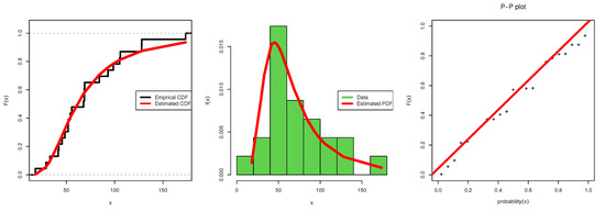
Figure 1. Estimated CDF, pdf, and pp-plot: data set I.

To check the performance of the MLE, we plot the profile likelihood function, where the x-label is one parameter with different values and the y-label is the log-likelihood value keeping the other parameters to be fixed. The profile likelihood of data set I is sketched in Figure 2, where the blue line is a log-likelihood values with different value of parameter and dot is the MLE estimator of parameter with max log-likelihood value, and it confirms that the MLE estimates have maximum values for data set I, which is consistent with the values of MLE observed in Table 2, and it is also clear that data set I behave very well as the three roots of the parameter are global maxima.

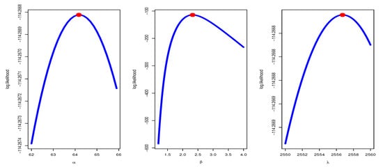
Figure 2. The Profile likelihood curve with maximum point for data set I.

The plots of the MCMC trace, the auto-correlation (ACF) tests, the posterior sample histogram, and the convergence of MCMC are all performed to diagnose the issues related to MCMC samples. An essential tool for evaluating a chain’s mixing is a trace plot. The auto-correlation plot, also known as the ACF plot, shows the serial correlation in time-varying data. Therefore, we plot MCMC trace, ACF plot, and a histogram of posterior density of MCMC results, and the convergence of the MCMC results for data set I are presented in Figure 3, Figure 4, Figure 5 and Figure 6, respectively.

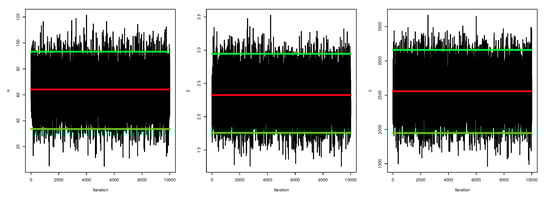
Figure 3. MCMC trace: data set I.

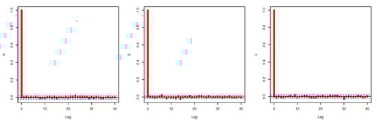
Figure 4. Auto-correlation test: data set I.

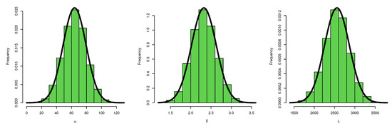
Figure 5. Histogram of posterior density: data set I.

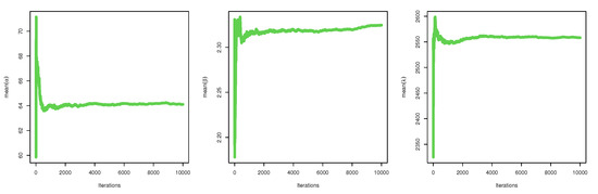
Figure 6. Convergence of MCMC results: data set I.

Figure 3, Figure 5, and Figure 6 confirm that the MCMC trace has normal results and convergence measures for data set I. Furthermore, this shows the histograms for the marginal posterior density estimates of the parameters based on 5000 chain values and the Gaussian kernel. The estimation in Figure 5 clearly indicates that all generated posteriors are symmetric with respect to the theoretical posterior density function. Figure 4 explores the auto-correlation test which revealed that the auto-correlation test for the MCMC is the correlation between an iteration series with a decreased version of itself. The auto-correlation function started to slow down at zero, which represents the correlation of the iteration series with itself, and then, it resulted in a correlation of one.

Table 3 provides the MLE, the MPS, and the Bayesian estimates for parameters of APIW distribution based on hybrid censored samples for data set I. Table 4 presents the survival and hazard of APIW distribution based on hybrid censored samples with data set I.

Table 3. MLE, MPS, and Bayesian estimates based on hybrid censored samples: data set I.

T	r		MLE		MPS		Bayesian
			Estimates	SE	Estimates	SE	Estimates	SE
68	12	$\alpha$	46.3400	163.7701	83.8863	351.3109	46.3076	3.9134
		$\beta$	1.9705	0.4337	1.6145	0.4176	1.9692	0.4331
		$\lambda$	747.1634	1407.1232	156.5471	329.6032	747.8127	156.7151
	16	$\alpha$	46.0169	162.8815	74.4494	322.0154	45.9893	3.2896
		$\beta$	1.9650	0.4308	2.0330	0.2510	1.9637	0.4302
		$\lambda$	733.8110	1375.322	745.4669	10.3476	734.6510	131.6786
110	16	$\alpha$	55.8774	166.4168	79.4264	16.2216	55.8488	3.2118
		$\beta$	2.1265	0.3848	1.8119	0.0638	2.1254	0.3742
		$\lambda$	1246.7484	2026.3962	320.7453	8.6051	1247.550	169.1073
	20	$\alpha$	60.7348	157.5242	75.2723	10.3590	60.7075	3.0404
		$\beta$	2.2491	0.3624	1.9606	0.0645	2.2480	0.3319
		$\lambda$	1935.9909	1875.5629	565.5794	10.3615	1937.155	139.9357

Table 4. Survival and hazard based on hybrid censored samples: data set I.

T	r		MLE	MPS	Bayesian
68	12	survival	0.4857	0.5113	0.4877
		hazard	0.0188	0.0150	0.0188
	16	survival	0.4850	0.5107	0.4869
		hazard	0.0188	0.0150	0.0187
110	16	survival	0.3253	0.3563	0.3268
		hazard	0.0197	0.0163	0.0197
	20	survival	0.1978	0.2277	0.1988
		hazard	0.0185	0.0158	0.0185

It is observed from the numerical results in Table 3 that the Bayesian estimators act better than alternative methods for estimating the parameter $\alpha$, while the MPS is the best choice for estimating the parameters $\beta$ and $\lambda$. Table 4 demonstrates the efficiency of the MPS estimation method since the survival estimation is maximized and the hazard rate estimation is minimized under the MPS estimation method.

6.2. Data Set II

A real data set II from Okash et al. [34] is considered. To demonstrate the reliability of the APIW distribution to fit these data, 72 observations of resistance in guinea pigs were exposed to various dosages of virulent tubercle bacilli. The observed data set II has been shown in Table 5.

Table 5. Survival times (in days) of resistance in guinea pigs exposed to various dosages of virulent tubercle bacilli.

12 38 55 60 70 85 121 211

15 38 56 61 72 87 127 233

22 43 57 62 73 91 129 258

24 44 58 63 75 95 131 258

24 48 58 65 76 96 143 263

32 52 59 65 76 98 146 297

32 53 60 67 81 99 146 341

33 54 60 68 83 109 175 341

Table 6 details MLE, MPS, and Bayesian estimates with SE and DKS goodness of fit test for data set II. While analyzing data set II, it is realized that the MPS estimates have lower SE values for the estimated APIW parameters. For modeling purposes, the Bayesian estimation has the minimum KSD (0.1091) and highest PVKS (0.3581); hence, the APIW distribution offers a better fit under Bayesian estimation. Figure 7 illustrates the APIW distribution’s theoretical and empirical $pdf$, CDF, and P-P plot using data set II, and it can be seen that the APIW is suitable and reliable for fitting data set II.

Table 6. MLE, MPS, and Bayesian estimates with SE values and KS test: data set II.

		Estimates	SE	Lower	Upper	KSD	PVKS
MLE	$\alpha$	99.0793	46.2628	8.4043	189.7544	0.1096	0.3524
	$\beta$	1.7889	0.1558	1.4835	2.0944
	$\lambda$	344.2289	143.1508	63.6533	624.8045
MPS	$\alpha$	122.7002	4.7472	113.3957	132.0046	0.1186	0.2637
	$\beta$	1.6840	0.0358	1.6139	1.7542
	$\lambda$	210.6960	2.5855	205.6284	215.7635
Bayesian	$\alpha$	98.9326	15.7863	68.4324	129.4730	0.1091	0.3581
	$\beta$	1.7885	0.1556	1.4991	2.1047
	$\lambda$	344.2667	24.3636	295.4979	392.3949

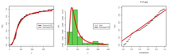
Figure 7. Estimated CDF, pdf and pp-plot: data set II.

Figure 8 confirms that the MLE estimates have the maximum likelihood values for data set II for the estimated parameter values that coincide with the MLE estimates in Table 6. Figure 9, describing the trace of the MCMC and its convergence. Figure 10 states that there is no auto-correlation for the MCMC series; the values started with zero and end up with one. In Figure 11, it is emphasized that the MCMC results have a normal curve with symmetric histograms of the posterior density, while Figure 12 shows that the MCMC trace has convergence results. Table 7 summarizes the MLE, the MPS, and the Bayesian estimates for parameters of APIW distribution based on hybrid censored samples for data set II with different values of T and r. The Bayesian estimators are better for estimating the parameter $\alpha$, while the MPS is the best choice for estimating the parameters $\beta$ and $\lambda$. Table 8 shows the estimated values of the survival and the hazard of APIW distribution based on the hybrid censored samples with data set II with different values of T and r. It is clear that the maximum survival is attained under MPS estimation and also the minimum hazard rate is obtained under MPS estimation, which supports the selection of the MPS method for efficient failure data analysis.

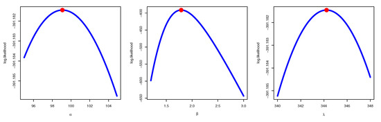
Figure 8. The Profile likelihood curve with the maximum point for data set II.

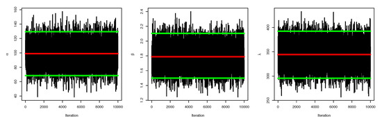
Figure 9. MCMC trace: data set II.

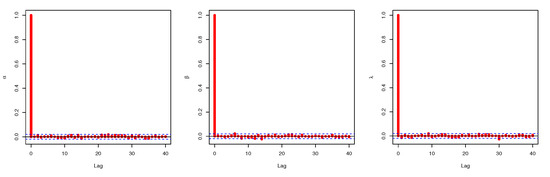
Figure 10. Auto-correlation test: data set II.

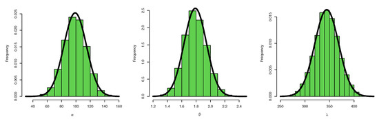
Figure 11. Histogram of posterior density: data set II.

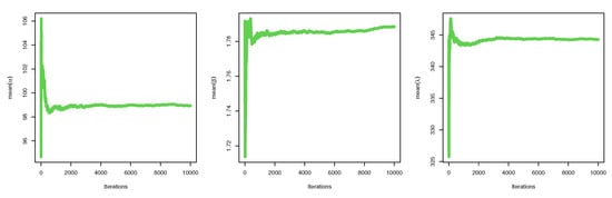
Figure 12. Convergence of MCMC results: data set II.

Table 7. MLE, MPS, and Bayesian estimates based on hybrid censored samples: data set II.

T	r		MLE		MPS		Bayesian
			Estimates	SE	Estimates	SE	Estimates	SE
100	50	$\alpha$	101.0733	164.6184	125.1150	67.7176	101.0304	3.9380
		$\beta$	1.7786	0.1811	1.6609	0.0656	1.7781	0.1809
		$\lambda$	327.2383	259.4398	191.2807	22.0057	327.2877	28.8832
	60	$\alpha$	103.0959	164.5881	126.4073	9.2812	103.0530	3.9373
		$\beta$	1.7976	0.1786	1.6819	0.0363	1.7970	0.1783
		$\lambda$	349.4182	271.6575	206.2780	5.2838	349.4698	30.2434
110	50	$\alpha$	101.0733	164.6184	125.1150	67.7176	101.0304	3.9380
		$\beta$	1.7786	0.1811	1.6609	0.0656	1.7781	0.1809
		$\lambda$	327.2383	259.4398	191.2807	22.0057	327.2877	28.8832
	60	$\alpha$	101.2719	164.0169	125.7735	16.0496	101.2291	3.9237
		$\beta$	1.7814	0.1748	1.6686	0.0365	1.7808	0.1745
		$\lambda$	330.4588	255.2788	196.5964	4.9556	330.5050	28.4200

Table 8. Survival and hazard based on hybrid censored samples: data set II.

T	r		MLE	MPS	Bayesian
100	50	survival	0.3523	0.3647	0.3530
		hazard	0.0141	0.0130	0.0141
	60	survival	0.3286	0.3412	0.3293
		hazard	0.0140	0.0130	0.0140
110	50	survival	0.3523	0.3647	0.3530
		hazard	0.0141	0.0130	0.0141
	60	survival	0.2906	0.3040	0.2912
		hazard	0.0131	0.0121	0.0131

7. A Simulation Study

A simulation analysis was carried out using 5000 iterations for hybrid Type-II censored samples. For the generated simulated sample from APIW distribution, descriptive statistics are computed to evaluate the consistency of this simulated data, Table 9 summarizes some measures in addition to skewness and kurtosis measures. Each simulation compares the APIW distribution parameter estimators by likelihood, product spacing, and Bayesian. Censored APIW samples are with the initial values:

Table 9. Summary of simulated data from APIW distribution.

$\mathit{\alpha }$	$\mathit{\beta }$	$\mathit{\lambda }$	Minimum	Q1	Q2	Mean	Q3	Maximum	SD	SK	KT
0.6	0.6	0.2	0.0019	0.0375	0.0968	9.3625	0.3837	2525.81	117.8092	17.2574	320.5176
		0.7	0.0341	0.2744	0.781	28.6615	3.2646	3533.482	188.5746	12.4815	188.0099
		1.2	0.0504	0.564	1.6943	554.9259	6.8621	373,379.5	12,016.08	30.0298	929.0447
		1.7	0.1445	1.1408	3.2773	112.0147	12.4232	25308.46	988.7543	18.8949	440.0531
		2.2	0.1183	1.7701	4.6629	758.7959	18.144	254,110.1	9603.757	21.2078	516.2217
		2.7	0.136	2.4891	7.0995	12,403.68	29.2255	621,3521	244,427.2	22.5586	527.7023
	1.5	0.2	0.0817	0.2689	0.3929	0.7271	0.6817	22.9594	1.492	9.6082	119.4912
		0.7	0.2587	0.5961	0.9059	1.6512	1.6052	26.2592	2.4575	4.8751	34.0851
		1.2	0.3026	0.7953	1.2348	2.449	2.1606	169.3792	7.1983	15.4838	314.6141
		1.7	0.4613	1.0541	1.6077	2.8005	2.7396	57.7173	4.1289	6.1401	56.8222
		2.2	0.4258	1.2566	1.8512	3.8492	3.1878	145.2141	8.8066	9.0808	110.2727
		2.7	0.4502	1.4402	2.1902	5.3273	3.8574	521.597	24.5777	16.9134	322.1059
	3	0.2	0.2859	0.5186	0.6269	0.7411	0.8256	4.7916	0.4218	4.1298	29.9656
		0.7	0.5087	0.7721	0.9518	1.1322	1.267	5.1244	0.608	2.6053	11.9396
		1.2	0.5501	0.8918	1.1112	1.3201	1.4699	13.0146	0.8409	5.8075	58.3727
		1.7	0.6792	1.0267	1.268	1.4908	1.6552	7.5972	0.7606	2.7864	14.7529
		2.2	0.6526	1.121	1.3606	1.662	1.7854	12.0505	1.0431	4.2566	29.2693
		2.7	0.671	1.2001	1.4799	1.8111	1.964	22.8385	1.4315	8.0332	97.9213
1.5	0.6	0.2	0.0021	0.0576	0.1675	20.1354	0.7441	5453.285	254.3222	17.2608	320.6308
		0.7	0.0395	0.4161	1.3517	61.1988	6.3512	7620.369	406.3593	12.502	188.5294
		1.2	0.0561	0.8339	2.8926	1196.982	13.2257	806,474.1	25,953.44	30.0314	929.1182
		1.7	0.167	1.7169	5.6449	239.0572	23.9633	54,604.49	2132.057	18.9211	441.0744
		2.2	0.1306	2.6675	7.9627	1633.918	34.8865	548,731.3	20,735.8	21.2142	516.483
		2.7	0.1484	3.7507	12.2307	26,786.65	56.6635	13,422,188	527,997	22.5588	527.7134
	1.5	0.2	0.0989	0.343	0.5117	0.9127	0.8951	25.1911	1.6971	8.8703	105.0283
		0.7	0.2976	0.7198	1.1197	1.9816	2.0002	28.5589	2.7859	4.5374	30.0123
		1.2	0.3396	0.9341	1.4893	2.8184	2.6335	164.0482	7.2539	14.1928	271.0224
		1.7	0.5111	1.2247	1.9137	3.2503	3.291	59.7669	4.4974	5.6013	48.348
		2.2	0.4661	1.4447	2.1772	4.3322	3.7888	141.9907	8.9929	8.4079	96.0569
		2.7	0.4889	1.6417	2.5574	5.7369	4.5445	470.9055	22.6724	16.1496	299.0034
	3	0.2	0.2912	0.5651	0.6995	0.8348	0.9426	5.589	0.502	4.0018	28.582
		0.7	0.5239	0.8392	1.0621	1.2755	1.4473	5.9758	0.7261	2.5326	11.4722
		1.2	0.5622	0.9643	1.2367	1.4842	1.676	15.1816	0.9981	5.6295	55.6979
		1.7	0.6991	1.1142	1.4136	1.6778	1.8876	8.8602	0.9095	2.6968	14.0562
		2.2	0.6655	1.2168	1.5143	1.8717	2.0348	14.0563	1.2387	4.1458	28.1226
		2.7	0.6828	1.3026	1.65	2.0412	2.2421	26.6419	1.6898	7.8521	94.6963
3	0.6	0.2	0.0023	0.0837	0.2587	33.3614	1.1989	9044.133	421.7753	17.2616	320.6565
		0.7	0.0453	0.5991	2.0877	101.2154	10.2436	12,634.96	673.6439	12.5066	188.6474
		1.2	0.062	1.1807	4.4402	1984.686	21.2686	1,337,645	43,047.07	30.0318	929.1349
		1.7	0.191	2.4597	8.6994	395.314	38.5459	90,546.07	3534.951	18.9271	441.3064
		2.2	0.1428	3.825	12.2242	2708.01	56.0588	910,095.2	34,390.2	21.2156	516.5424
		2.7	0.1605	5.3781	18.8508	44,427.34	91.2935	22,263,025	875,773	22.5589	527.7159
	1.5	0.2	0.102	0.3945	0.6023	1.0877	1.0704	30.4535	2.0548	8.8479	104.636
		0.7	0.3133	0.8252	1.3179	2.3613	2.3929	34.5215	3.3769	4.5215	29.8511
		1.2	0.3524	1.0643	1.7489	3.3579	3.147	198.3252	8.7774	14.1699	270.3686
		1.7	0.5375	1.4015	2.2507	3.869	3.9332	72.248	5.4519	5.5778	48.0366
		2.2	0.4819	1.6538	2.5569	5.1663	4.5263	171.6554	10.8861	8.3911	95.7611
		2.7	0.5035	1.8793	3.0078	6.855	5.4345	569.3038	27.4201	16.1402	298.7514
	3	0.2	0.296	0.6089	0.7631	0.9119	1.037	6.1841	0.5605	3.9338	27.9076
		0.7	0.5385	0.9026	1.1586	1.3933	1.5925	6.6117	0.8119	2.4899	11.2289
		1.2	0.5734	1.0338	1.3473	1.6196	1.8431	16.7984	1.1133	5.5364	54.3872
		1.7	0.7182	1.1972	1.5413	1.8319	2.0758	9.8033	1.0177	2.6452	13.7014
		2.2	0.6775	1.3078	1.6498	2.0443	2.2373	15.5531	1.3815	4.0881	27.5711
		2.7	0.6935	1.4	1.7991	2.2299	2.4665	29.4793	1.8797	7.7641	93.1916

• In Table 10: $\alpha =0.6,\beta =0.6,\lambda =0.7$ and $\alpha =1.3,\beta =0.6,\lambda =0.7$.
  Table 10. Bayesian and non-Bayesian estimation for parameters of APIW distribution based on hybrid censored samples where $\beta =0.6,\theta =0.7$.

  $\mathit{\beta }=0.6,\mathit{\theta }=0.7$					MLE					MPS					Bayesian
  $\mathbf{\alpha }$	n	T	r		RB	MSE	LACI	LBP	LBT	RB	MSE	LACI	LBP	LBT	RB	MSE	LCCI
  1.3	50	1.4	30	$\alpha$	0.0012	0.0791	1.1039	0.0476	0.0483	−0.0249	0.0679	1.0143	0.0437	0.0464	0.0748	0.0256	0.5025
  				$\beta$	0.0365	0.0108	0.3989	0.0199	0.0199	−0.0496	0.0100	0.3743	0.0167	0.0167	−0.2786	0.0091	0.4369
  				$\lambda$	0.0200	0.0255	0.6239	0.0298	0.0298	0.0520	0.0264	0.6212	0.0302	0.0318	−0.2234	0.0240	0.4759
  		7	40	$\alpha$	0.0010	0.0619	1.0723	0.0479	0.0479	−0.0024	0.0176	1.0065	0.0372	0.0371	0.0627	0.0178	0.4171
  				$\beta$	0.0267	0.0070	0.3228	0.0146	0.0148	−0.0412	0.0066	0.3030	0.0139	0.0135	−0.2631	0.0061	0.3763
  				$\lambda$	0.0182	0.0219	0.5790	0.0244	0.0239	0.0309	0.0235	0.5961	0.0249	0.0248	−0.2190	0.0140	0.3908
  		999	50	$\alpha$	−0.0014	0.0507	0.9554	0.0386	0.0468	−0.0019	0.0125	0.9899	0.0287	0.0288	0.0313	0.0073	0.2778
  				$\beta$	0.0102	0.0053	0.2839	0.0119	0.0120	−0.0416	0.0058	0.2590	0.0107	0.0108	−0.2344	0.0046	0.2703
  				$\lambda$	0.0162	0.0204	0.4719	0.0233	0.0233	0.0291	0.0214	0.5761	0.0237	0.0237	−0.2109	0.0128	0.2981
  	100	1.4	70	$\alpha$	0.0360	0.2776	2.0930	0.1478	0.1481	−0.0577	0.1186	1.3516	0.0622	0.0625	0.1368	0.0470	0.4726
  				$\beta$	0.0195	0.0043	0.2520	0.0119	0.0119	−0.0311	0.0045	0.2529	0.0116	0.0115	−0.3606	0.0016	0.3682
  				$\lambda$	0.0083	0.0211	0.4019	0.0273	0.0172	0.0316	0.0143	0.4616	0.0211	0.0212	−0.3061	0.0155	0.3704
  		7	90	$\alpha$	0.0308	0.2697	1.9132	0.1309	0.0908	0.0405	0.1041	1.2503	0.0611	0.0611	0.1163	0.0344	0.4199
  				$\beta$	0.0101	0.0039	0.2443	0.0101	0.0101	−0.0304	0.0042	0.2455	0.0111	0.0109	−0.4388	0.0015	0.3200
  				$\lambda$	0.0318	0.0197	0.3944	0.0234	0.0162	0.0314	0.0123	0.3602	0.0202	0.0209	−0.4305	0.0150	0.3220
  		999	100	$\alpha$	0.0428	0.2500	1.7648	0.1216	0.0812	−0.0401	0.0985	1.2854	0.0513	0.0513	0.0623	0.0114	0.2600
  				$\beta$	−0.0045	0.0038	0.2419	0.0091	0.0100	−0.0316	0.0042	0.2354	0.0107	0.0106	−0.3557	0.0009	0.2399
  				$\lambda$	0.0263	0.0137	0.3735	0.0213	0.0133	0.0291	0.0106	0.3488	0.0200	0.0237	−0.3547	0.0114	0.2948
  0.6	50	0.5	30	$\alpha$	0.0616	0.0412	0.7829	0.0350	0.0348	−0.0301	0.0370	0.7512	0.0352	0.0355	0.1988	0.0290	0.4688
  				$\beta$	0.0596	0.0126	0.4182	0.0194	0.0195	−0.0571	0.0106	0.3818	0.0166	0.0166	−0.1291	0.0106	0.3893
  				$\lambda$	−0.0187	0.0261	0.6321	0.0271	0.0272	0.0902	0.0374	0.7172	0.0312	0.0308	−0.1567	0.0128	0.5101
  		5	40	$\alpha$	0.0577	0.0417	0.7004	0.0344	0.0315	−0.0301	0.0353	0.6903	0.0341	0.0341	0.1239	0.0283	0.3812
  				$\beta$	0.0320	0.0079	0.3413	0.0157	0.0159	−0.0493	0.0072	0.3116	0.0143	0.0143	−0.1234	0.0079	0.3346
  				$\lambda$	0.0106	0.0257	0.6404	0.0260	0.0270	0.0752	0.0330	0.6827	0.0279	0.0277	−0.1271	0.0125	0.3717
  		99,999	50	$\alpha$	0.1308	0.0125	0.6835	0.0316	0.0259	−0.0280	0.0311	0.5259	0.0354	0.0255	0.1137	0.0121	0.2803
  				$\beta$	0.0335	0.0068	0.3139	0.0141	0.0144	−0.0467	0.0070	0.2986	0.0141	0.0137	−0.1197	0.0069	0.2393
  				$\lambda$	0.0064	0.0231	0.6191	0.0213	0.0231	0.0612	0.0349	0.6180	0.0238	0.0238	−0.1090	0.0102	0.3190
  	100	0.5	70	$\alpha$	0.1568	0.1709	1.5798	0.0743	0.0745	−0.0893	0.1224	1.3568	0.0605	0.0605	0.3783	0.0640	0.4302
  				$\beta$	0.0221	0.0086	0.3598	0.0154	0.0154	−0.0714	0.0096	0.3456	0.0164	0.0161	−0.1407	0.0091	0.3560
  				$\lambda$	0.0357	0.0532	0.8997	0.0411	0.0408	0.1771	0.0779	0.9813	0.0448	0.0448	−0.2168	0.0351	0.4293
  		5	90	$\alpha$	0.2180	0.1523	1.2823	0.0750	0.0682	0.0120	0.1182	1.3675	0.0607	0.0602	0.3728	0.0618	0.3257
  				$\beta$	0.0170	0.0044	0.2584	0.0110	0.0111	−0.0487	0.0054	0.2634	0.0123	0.0126	−0.1287	0.0036	0.2954
  				$\lambda$	0.0075	0.0344	0.7277	0.0330	0.0329	0.1039	0.0532	0.8592	0.0391	0.0398	−0.2042	0.0294	0.3247
  		99,999	100	$\alpha$	0.1976	0.1224	1.2799	0.0677	0.0658	−0.0169	0.1022	1.2844	0.0585	0.0588	0.2379	0.0244	0.2489
  				$\beta$	0.0124	0.0042	0.2468	0.0102	0.0102	−0.0371	0.0047	0.2484	0.0123	0.0123	−0.1264	0.0035	0.2385
  				$\lambda$	0.0226	0.0315	0.7310	0.0318	0.0319	0.1007	0.0471	0.7933	0.0342	0.0342	−0.1321	0.0156	0.3095

• In Table 11: $\alpha =0.6,\beta =0.6,\lambda =2$ and $\alpha =2,\beta =0.6,\lambda =2$.
  Table 11. Bayesian and non-Bayesian estimation for parameters of APIW distribution based on hybrid censored samples where $\beta =0.6,\theta =2$.

  $\mathit{\beta }=0.6,\mathit{\theta }=2$					MLE					MPS					Bayesian
  $\mathbf{\alpha }$	n	T	r		RB	MSE	LACI	LBP	LBT	RB	MSE	LACI	LBP	LBT	RB	MSE	LCCI
  0.6	50	1.4	30	$\alpha$	0.5022	0.6443	2.9192	0.1332	0.1314	0.1281	0.5495	2.8997	0.1347	0.1377	0.1649	0.0247	0.4886
  				$\beta$	0.0198	0.0100	0.3889	0.0179	0.0198	−0.1065	0.0135	0.3808	0.0179	0.0177	−0.3502	0.0095	0.3791
  				$\lambda$	0.0087	0.2139	1.8136	0.0792	0.0792	0.0566	0.2394	1.8677	0.0874	0.0867	−0.0478	0.0295	0.5636
  		7	40	$\alpha$	0.5263	0.6337	2.8674	0.1257	0.1282	0.1210	0.4745	2.6878	0.1160	0.1163	0.1672	0.0216	0.4103
  				$\beta$	0.0547	0.0091	0.3410	0.0169	0.0185	−0.0678	0.0128	0.3414	0.0178	0.0181	−0.3339	0.0085	0.2883
  				$\lambda$	−0.0097	0.1465	1.4999	0.0718	0.0725	0.0304	0.1519	1.5104	0.0703	0.0700	−0.0326	0.0241	0.4540
  		999	50	$\alpha$	0.1792	0.1318	1.3605	0.0603	0.0607	−0.1141	0.1057	1.2317	0.0537	0.0545	0.1095	0.0096	0.2808
  				$\beta$	0.0535	0.0081	0.3249	0.0159	0.0172	−0.0579	0.0126	0.3246	0.0168	0.0172	−0.2406	0.0062	0.2289
  				$\lambda$	0.0389	0.1410	1.4413	0.0648	0.0651	0.0302	0.1495	1.4070	0.0613	0.0598	−0.0301	0.0098	0.2934
  	100	1.4	70	$\alpha$	0.1216	0.1193	1.3246	0.0623	0.0652	−0.1856	0.0907	1.0981	0.0497	0.0497	0.2768	0.0400	0.4275
  				$\beta$	0.0154	0.0074	0.3355	0.0153	0.0153	−0.0829	0.0088	0.3113	0.0124	0.0125	−0.5069	0.0070	0.2629
  				$\lambda$	0.0214	0.0974	1.2132	0.0568	0.0604	0.0675	0.1189	1.2450	0.0545	0.0545	−0.0894	0.0496	0.5074
  		7	90	$\alpha$	0.1407	0.1028	1.2361	0.0614	0.0620	−0.0333	0.0787	1.0978	0.0451	0.0496	0.2681	0.0384	0.3780
  				$\beta$	0.0190	0.0050	0.2728	0.0119	0.0120	−0.0413	0.0051	0.2624	0.0116	0.0121	−0.4668	0.0048	0.2168
  				$\lambda$	0.0001	0.0430	1.1381	0.0361	0.0368	0.0078	0.0413	0.7955	0.0355	0.0355	−0.0891	0.0145	0.4277
  		999	100	$\alpha$	0.0442	0.0941	1.1989	0.0546	0.0550	−0.0220	0.0611	1.0021	0.0436	0.0456	0.1824	0.0168	0.2568
  				$\beta$	0.0031	0.0042	0.2554	0.0106	0.0107	−0.0181	0.0048	0.2488	0.0103	0.0112	−0.3617	0.0025	0.1912
  				$\lambda$	0.0275	0.0372	1.0306	0.0346	0.0346	0.0072	0.0412	0.6226	0.0305	0.0315	−0.0541	0.0138	0.3084
  2	50	4	30	$\alpha$	−0.0049	0.8570	3.6322	0.1661	0.1670	−0.0257	0.8294	3.5679	0.1661	0.1658	0.0166	0.0233	0.5513
  				$\beta$	0.0138	0.0083	0.2758	0.0131	0.0127	−0.0575	0.0054	0.2558	0.0112	0.0152	−0.2798	0.0078	0.3962
  				$\lambda$	0.0657	0.1980	1.6680	0.0756	0.0754	−0.0072	0.1540	1.5390	0.0704	0.0701	−0.0401	0.0252	0.5318
  		22	40	$\alpha$	0.0194	0.4354	2.5847	0.1154	0.1161	0.0256	0.5350	2.8432	0.1193	0.1216	0.0159	0.0131	0.4276
  				$\beta$	0.0253	0.0068	0.2319	0.0125	0.0121	−0.0430	0.0046	0.2305	0.0110	0.0142	−0.2492	0.0064	0.2740
  				$\lambda$	0.0454	0.1786	1.6195	0.0749	0.0716	−0.0092	0.1392	1.4333	0.0655	0.0653	−0.0470	0.0232	0.4449
  		99,999	50	$\alpha$	0.0068	0.0965	1.2178	0.0534	0.0535	−0.0116	0.1648	1.5901	0.0698	0.0694	0.0132	0.0064	0.2937
  				$\beta$	0.0597	0.0062	0.2137	0.0116	0.0110	−0.0357	0.0030	0.2155	0.0195	0.0135	−0.2189	0.0052	0.2133
  				$\lambda$	0.0522	0.1581	0.8506	0.0709	0.0691	−0.0062	0.1013	1.2392	0.0558	0.0551	−0.0328	0.0106	0.3105
  	100	4	70	$\alpha$	0.0254	0.4205	2.5368	0.1136	0.1155	−0.0166	0.2736	2.0482	0.0951	0.0953	0.0236	0.0187	0.4739
  				$\beta$	0.0297	0.0084	0.3525	0.0157	0.0158	−0.0443	0.0079	0.3325	0.0151	0.0152	−0.4132	0.0068	0.3206
  				$\lambda$	0.0263	0.0757	1.0599	0.0477	0.0474	−0.0081	0.0649	0.9977	0.0460	0.0472	−0.0764	0.0431	0.5429
  		22	90	$\alpha$	−0.0065	0.0729	1.0584	0.0463	0.0453	−0.0135	0.0375	0.7523	0.0323	0.0322	0.0210	0.0157	0.4303
  				$\beta$	0.0131	0.0032	0.2204	0.0099	0.0100	−0.0286	0.0033	0.2136	0.0096	0.0095	−0.4079	0.0016	0.2093
  				$\lambda$	0.0255	0.0650	0.9804	0.0449	0.0450	−0.0081	0.0540	0.9009	0.0405	0.0405	−0.0696	0.0410	0.4314
  		99,999	100	$\alpha$	0.0028	0.0629	1.0104	0.0390	0.0389	0.0124	0.0246	0.5092	0.0319	0.0239	0.0213	0.0082	0.2936
  				$\beta$	0.0066	0.0027	0.2032	0.0097	0.0095	−0.0236	0.0033	0.2080	0.0092	0.0092	−0.3042	0.0011	0.1713
  				$\lambda$	0.0163	0.0579	0.9094	0.0436	0.0426	−0.0072	0.0485	0.8127	0.0353	0.0395	−0.0621	0.0215	0.3091

• In Table 12: $\alpha =0.8,\beta =2,\lambda =2$ and $\alpha =2,\beta =2,\lambda =2$.
  Table 12. Bayesian and non-Bayesian estimation for parameters of APIW distribution based on hybrid censored samples where $\beta =2,\theta =2$.

  $\mathit{\beta }=2,\mathit{\theta }=2$					MLE					MPS					Bayesian
  $\mathbf{\alpha }$	n	T	r		RB	MSE	LACI	LBP	LBT	RB	MSE	LACI	LBP	LBT	RB	MSE	LCCI
  0.8	50	1.5	30	$\alpha$	0.3767	0.7387	3.1630	0.2334	0.2282	−0.1050	0.4568	2.6352	0.1943	0.1950	0.1140	0.0253	0.5532
  				$\beta$	0.0402	0.2281	1.8497	0.1278	0.1290	−0.1186	0.2520	1.7381	0.1227	0.1230	−0.0496	0.0303	0.5508
  				$\lambda$	0.0631	0.3817	2.3764	0.1554	0.1548	0.1214	0.3962	2.2821	0.1698	0.1678	−0.0505	0.0310	0.6040
  		3	40	$\alpha$	0.3105	0.6978	3.0153	0.2033	0.2013	0.1029	0.4169	2.6153	0.1820	0.2934	0.1240	0.0211	0.4089
  				$\beta$	0.0495	0.1812	1.6247	0.0694	0.0687	−0.0569	0.1871	1.6375	0.0732	0.0738	−0.0484	0.0214	0.4397
  				$\lambda$	−0.0143	0.2779	2.0654	0.0892	0.0886	0.0860	0.3350	2.2711	0.1008	0.1019	−0.0502	0.0249	0.4433
  		99	50	$\alpha$	0.2901	0.6495	2.6126	0.1931	0.1873	0.1026	0.4053	2.5852	0.1830	0.1830	0.0791	0.0094	0.2958
  				$\beta$	0.0211	0.1413	1.4660	0.0672	0.0667	−0.0512	0.1822	1.5636	0.0726	0.0777	−0.0279	0.0089	0.2905
  				$\lambda$	0.0131	0.2533	2.0125	0.0820	0.0830	0.0092	0.2464	2.0574	0.0711	0.0710	−0.0305	0.0104	0.3250
  	100	1.5	70	$\alpha$	0.3635	0.6536	2.9600	0.1373	0.1360	−0.0689	0.5129	2.8018	0.1278	0.1259	0.1916	0.0383	0.4662
  				$\beta$	0.0276	0.1214	1.3497	0.0604	0.0585	−0.0964	0.1572	1.3598	0.0586	0.0589	−0.0749	0.0426	0.5332
  				$\lambda$	0.0189	0.2072	1.7800	0.0849	0.0864	0.1073	0.2985	1.9715	0.0853	0.0872	−0.0803	0.0451	0.5308
  		3	90	$\alpha$	0.3467	0.6173	2.3847	0.1241	0.1129	0.0598	0.4938	2.7555	0.1218	0.1128	0.1924	0.0453	0.3753
  				$\beta$	0.0129	0.0916	1.1830	0.0551	0.0553	−0.0558	0.1249	1.3158	0.0585	0.0589	−0.0718	0.0393	0.3852
  				$\lambda$	0.0248	0.2013	1.6856	0.0823	0.0825	0.0462	0.3020	1.9125	0.0799	0.0878	−0.0791	0.0462	0.4199
  		99	100	$\alpha$	0.2929	0.5981	2.1152	0.1127	0.1113	0.0463	0.4866	2.3417	0.1206	0.1027	0.1378	0.0171	0.2769
  				$\beta$	0.0152	0.0916	1.1818	0.0523	0.0523	−0.0479	0.1140	1.3319	0.0580	0.0561	−0.0549	0.0179	0.2981
  				$\lambda$	−0.0062	0.1928	1.6020	0.0819	0.0810	0.0458	0.3008	1.8910	0.0798	0.0799	−0.0534	0.0177	0.3142
  2	50	2	30	$\alpha$	0.1108	2.1771	5.7241	0.2747	0.2759	0.1555	3.6273	7.3730	0.3179	0.3503	0.0246	0.0212	0.5163
  				$\beta$	0.0198	0.1346	1.4314	0.0680	0.0668	−0.0698	0.1504	1.4197	0.0647	0.0647	−0.0524	0.0317	0.5489
  				$\lambda$	0.0679	0.2229	1.7742	0.0785	0.0785	0.0013	0.1940	1.7283	0.0803	0.0774	−0.0535	0.0339	0.5863
  		4	40	$\alpha$	0.1034	1.0666	4.2958	0.2410	0.2312	0.1426	3.4818	6.6843	0.3142	0.3227	0.0236	0.0151	0.4241
  				$\beta$	0.0055	0.1049	1.2701	0.0589	0.0590	−0.0623	0.1218	1.2788	0.0587	0.0600	−0.0497	0.0220	0.4423
  				$\lambda$	0.0881	0.2039	1.3575	0.0711	0.0781	0.0013	0.1837	1.6395	0.0801	0.0691	−0.0524	0.0253	0.4364
  		99	50	$\alpha$	0.0924	0.9740	4.0544	0.2419	0.2147	0.1448	3.0179	5.8231	0.2763	0.3081	0.0151	0.0075	0.3239
  				$\beta$	−0.0106	0.1007	1.2482	0.0577	0.0575	−0.0610	0.1161	1.1344	0.0575	0.0572	−0.0312	0.0104	0.3003
  				$\lambda$	0.1231	0.1504	1.1614	0.0612	0.0612	0.0019	0.1853	1.4771	0.0361	0.0611	−0.0289	0.0099	0.3013
  	100	2	70	$\alpha$	0.0622	1.2694	4.3940	0.1994	0.1961	0.0554	1.4031	4.6277	0.1925	0.1922	0.0492	0.0269	0.5138
  				$\beta$	−0.0048	0.0576	0.9413	0.0446	0.0447	−0.0582	0.0725	0.9522	0.0446	0.0443	−0.0921	0.0513	0.5276
  				$\lambda$	0.0432	0.1285	1.3653	0.0648	0.0645	0.0080	0.1371	1.4517	0.0694	0.0689	−0.0955	0.0556	0.5253
  		4	90	$\alpha$	0.0522	0.9516	2.2214	0.1909	0.1900	0.0512	0.9671	2.0285	0.1832	0.1823	0.0483	0.0211	0.4262
  				$\beta$	−0.0227	0.0583	0.9304	0.0407	0.0400	−0.0600	0.0772	0.9828	0.0462	0.0462	−0.0868	0.0407	0.4078
  				$\lambda$	0.0907	0.1267	1.0897	0.0618	0.0584	0.0074	0.1285	0.1064	0.0592	0.0590	−0.1036	0.0554	0.4244
  		99	100	$\alpha$	0.0413	0.9290	1.6319	0.1897	0.1880	0.0501	0.9155	2.0033	0.1733	0.1633	0.0277	0.0095	0.3026
  				$\beta$	−0.0144	0.0582	0.9397	0.0394	0.0395	−0.0617	0.0695	0.9060	0.0451	0.0451	−0.0534	0.0175	0.2841
  				$\lambda$	0.0831	0.1133	0.9915	0.0619	0.0493	0.0041	0.1141	0.1005	0.0411	0.0401	−0.0552	0.0184	0.3156

For the development of a hybrid censored sample, we selected different sample sizes as n = 50 and 100 and different censored sample sizes as r = 30, 40, and 50 for n = 50, r = 70, 90, and 100 for n = 100.

The relative bias (RB), mean square error (MSE), length of asymptotic confidence intervals (LACI), length of bootstrap-p (LBP), and length of bootstrap-t (LBT) are calculated, and a comparison was considered between the different approaches of the resulting estimators with respect to the RB of $\alpha ,\beta$, and $\lambda$. In addition, the MSE was utilized for the same purpose such that $MSE\left({\psi }_k\right)=\frac{1}{M}{\sum }_{i=1}^M{\left({\widehat{\psi }}_k^{\left(i\right)}-{\psi }_k\right)}^2,$ where $M=5000$ is the number of simulated samples, and $({\psi }_1=\alpha ,{\psi }_2=\beta ,{\psi }_3=\lambda )$. Overall, $95\%$ of the CIs are obtained from asymptotic distributions from MLEs and CRIs and are also compared with a further criterion. The comparison is between the average confidence interval length (ACL). In order to assess the type of prior, estimates of the parameters in the Bayes technique are computed from informative priors. The hyperparameters in the case of informative priors are chosen by elective hyperparameters using MLE information to show the results of estimated parameters.

From the simulation analysis, we point out the following results:

• The RB and the MSE decrease for estimated parameters of MLE and MPS as the sample size increases and the Bayes estimates for $\alpha$, $\beta$and $\lambda$ attain the minimum MSE. See Table 10, Table 11 and Table 12.
• In almost all cases, the Bayes estimates perform better than the MLEs with respect to RB, MSE, LACI, LBP, and LBT.
• In most cases, the MPS estimates are better than the MLE with respect to MSE.
• The performance increases when the censored sample size r increases, such that the sample size n and the time of the hybrid censored sample are kept fixed.
• The performance increases when the time of a hybrid censored sample increases when keeping sample size n and censored sample size r as fixed values.
• When the number of failures r is fixed and sample size n increases, the MSEs and width of the LACI, LBP, and LBT of the MLEs, MPS, and Bayes estimations are decreased. However, the MPS process performs well in terms of estimating the parameters of APIW. See Table 10, Table 11 and Table 12.
• The MSEs and the widths of the confidence intervals of the ACI, BP, and BT of the MLEs, MPS, and Bayes estimations decrease as the number of failures r increases for a fixed sample size n.
• As the sample size n increases, the average length of all intervals decreases. On average, the credible CI estimates are better than the ACI.
• As the sample size n increases, the bootstrap CI estimates are better than the traditional CI.

8. Conclusions

Modeling some biomedical data was performed in this study, the new APIW continuous distribution was utilized and the hybrid Type-II censoring scheme was recommended. Three estimation methods were performed to estimate the unknown parameters of the APIW distribution and hence estimate the survival and hazard functions. In real data analysis, the classical alternative (MPS) for the well-known MLE method confirmed the power fullness of the MPS over the MLE for estimating parameters, survival, and hazard function. In simulation analysis, the Bayesian approach for the inference of APIW parameters was relatively acting much better compared to the classical methods. A comparison was conducted with respect to the mean squared error and relative bias, and all results were summarized in tables and plotted in figures. The MCMC approach was employed as estimates from Bayesian are not directly obtainable. The model was applied to two real-life data sets, including failure statistical data for certain ball-bearing components and the resistance in guinea pigs exposed to various dosages of virulent tubercle bacilli.

References

- Ghalme, S.G.; Mankar, A.; Bhalerao, Y. Biomaterials in Hip Joint Replacement. Int. J. Mater. Sci. Eng. 2016, 4, 113–125. [Google Scholar] [CrossRef]
- Kochi, A. The global tuberculosis situation and the new control strategy of the World Health Organization. Tubercle 1991, 72, 1–6. [Google Scholar] [CrossRef]
- Epstein, B. Truncated life tests in the exponential case. Ann. Socite Pol. Math. 1954, 25, 555–564. [Google Scholar] [CrossRef]
- Ebrahimi, N. Estimating the parameters of an exponential distribution from hybrid life test. J. Stat. Plan. Inference 1986, 14, 255–261. [Google Scholar] [CrossRef]
- Childs, A.; Chand Rasekhar, B.; Balakrishnan, N.; Kundu, D.E. Likelihood inference based on type-I and type-II hybrid censored samples from the exponential distribution. Ann. Inst. Stat. Math. 2003, 55, 319–330. [Google Scholar] [CrossRef]
- Mansour, M.M.M.; Ramadan, D.A. Statistical inference of the parameters of the modified extended exponential distribution under the type-II hybrid censoring scheme. J. Appl. Probab. Stat. 2020, 15, 19–44. [Google Scholar]
- Salah, M.M.; Ahmed, E.A.; Alhussain, Z.A.; Ahmed, H.H.; El-Morshedy, M.; Eliwa, M.S. Statistical inferences for type-II hybrid censoring data from the alpha power exponential distribution. PLoS ONE 2021, 16, e0244316. [Google Scholar] [CrossRef] [PubMed]
- Yousef, M.M.; Almetwally, E.M. Bayesian Inference for the Parameters of Exponential Chen Distribution Based on Hybrid Censoring. Pak. J. Stat. 2022, 38, 145–164. [Google Scholar]
- Yadav, A.S.; Singh, S.K.; Singh, U. On hybrid censored inverse Lomax distribution: Application to the survival data. Statistica 2016, 76, 185–203. [Google Scholar]
- Mahmoud, M.A.W.; Ramadan, D.A.; Mansour, M.M.M. Estimation of lifetime parameters of the modified extended exponential distribution with application to a mechanical model. Commun. Stat. Simul. Comput. 2020, 51, 7005–7018. [Google Scholar] [CrossRef]
- Aldahlan, M.A.; Bakoban, R.A.; Alzahrani, L.S. On Estimating the Parameters of the Beta Inverted Exponential Distribution under Type-II Censored Samples. Mathematics 2022, 10, 506. [Google Scholar] [CrossRef]
- Mohammed, H.S.; Nassar, M.; Alotaibi, R.; Elshahhat, A. Analysis of Adaptive Progressive Type-II Hybrid Censored Dagum Data with Applications. Symmetry 2022, 14, 2146. [Google Scholar] [CrossRef]
- Ramadan, D.A.; Aboshady, M.S.; Mansour, M.M.M. Inference for modified extended exponential distribution based on progressively Type-I hybrid censored data with application to some mechanical models. J. Appl. Probab. Stat. 2022, 17, 69–88. [Google Scholar]
- Nassr, S.G.; Almetwally, E.M.; El Azm, W.S.A. Statistical inference for the extended weibull distribution based on adaptive type-II progressive hybrid censored competing risks data. Thail. Stat. 2021, 19, 547–564. [Google Scholar]
- Ramadan, D.A.; Magdy, W.A. On the alpha-power inverse Weibull. Int. J. Comput. Appl. 2018, 181, 975–8887. [Google Scholar]
- El-Sagheer, R.M. Estimation of parameters of Weibull-Gamma distribution based on progressively censored data. Stat. Pap. 2018, 59, 725–757. [Google Scholar] [CrossRef]
- Cheng, R.C.H.; Amin, N.A.K. Estimating parameters in continuous univariate distributions with a shifted origin. J. R. Stat. Soc. Ser. B Methodol. 1983, 45, 394–403. [Google Scholar] [CrossRef]
- Kundu, D.; Howlader, H. Bayesian inference and prediction of the inverse Weibull distribution for Type-II censored data. Comput. Stat. Data Anal. 2010, 54, 1547–1558. [Google Scholar] [CrossRef]
- Dey, S.; Dey, T. On progressively censored generalized inverted exponential distribution. J. Appl. Stat. 2014, 41, 2557–2576. [Google Scholar] [CrossRef]
- Dey, S.; Ali, S.; Park, C. Weighted exponential distribution: Properties and different methods of estimation. J. Stat. Comput. Simul. 2015, 85, 3641–3661. [Google Scholar] [CrossRef]
- Dey, S.; Singh, S.; Tripathi, Y.M.; Asgharzadeh, A. Estimation and prediction for a progressively censored generalized inverted exponential distribution. Stat. Methodol. 2016, 32, 185–202. [Google Scholar] [CrossRef]
- Varian, H.R. Bayesian approach to real estate assessment. In Studies in Bayesian Econometrics and Statistics in Honor of L.J. Savage; Feinderg, S.E., Zellner, A., Eds.; North-Holland: Amsterdam, The Netherlands, 1975; pp. 195–208. [Google Scholar]
- Robert, C.P. Monte Carlo Statistical Methods; Springer: New York, NY, USA, 2004. [Google Scholar]
- Tolba, A. Bayesian and Non-Bayesian Estimation Methods for Simulating the Parameter of the Akshaya Distribution. Comput. J. Math. Stat. Sci. 2022, 1, 13–25. [Google Scholar] [CrossRef]
- Lawless, J.F. Statistical Models and Methods for Lifetime Data; John Wiley and Sons: New York, NY, USA, 1982. [Google Scholar]
- Greene, W.H. Econometric Analysis, 4th ed.; Prentice-Hall: NewYork, NY, USA, 2000. [Google Scholar]
- Meeker, W.Q.; Escobar, L.A. Statistical Methods for Reliability Data; Wiley: New York, NY, USA, 1998. [Google Scholar]
- Efron, B. The bootstrap and other resampling plans. In CBMS-NSF Regional Conference Series in Applied Mathematics; SIAM: Philadelphia, PA, USA, 1982. [Google Scholar]
- Hall, P. Theoretical Comparison of Bootstrap Confidence Intervals. Ann. Stat. 1988, 16, 927–953. [Google Scholar] [CrossRef]
- Almongy, H.M.; Almetwally, E.M.; Alharbi, R.; Alnagar, D.; Hafez, E.H.; Mohie El-Din, M.M. The Weibull generalized exponential distribution with censored sample: Estimation and application on real data. Complexity 2021, 2021, 6653534. [Google Scholar] [CrossRef]
- Muhammed, H.Z.; Almetwally, E.M. Bayesian and non-Bayesian estimation for the bivariate inverse weibull distribution under progressive type-II censoring. Ann. Data Sci. 2020, 1–32. [Google Scholar] [CrossRef]
- Balakrishnan, N.; Sandhu, R.A. Best linear unbiased and maximum likelihood estimation for exponential distributions under general progressive Type-ll censored samples. Indian J. Stat. Ser. B 1996, 58, 1–9. [Google Scholar]
- Leiblein, J.; Zelen, M. Statistical investigation of fatigue life of deep groove ball bearings. Res. Natl. Bur. Stand. 1956, 57, 273–316. [Google Scholar] [CrossRef]
- Okasha, H.M.; El-Baz, A.H.; Tarabia, A.M.K.; Basheer, A.M. Extended inverse weibull distribution with reliability application. J. Egypt. Math. Soc. 2017, 25, 343–349. [Google Scholar] [CrossRef]
Disclaimer/Publisher’s Note: The statements, opinions and data contained in all publications are solely those of the individual author(s) and contributor(s) and not of MDPI and/or the editor(s). MDPI and/or the editor(s) disclaim responsibility for any injury to people or property resulting from any ideas, methods, instructions or products referred to in the content. |
© 2023 by the authors. Licensee MDPI, Basel, Switzerland. This article is an open access article distributed under the terms and conditions of the Creative Commons Attribution (CC BY) license (https://creativecommons.org/licenses/by/4.0/).