Conjugate Gradient Algorithm for Least-Squares Solutions of a Generalized Sylvester-Transpose Matrix Equation

Abstract

We derive a conjugate-gradient type algorithm to produce approximate least-squares (LS) solutions for an inconsistent generalized Sylvester-transpose matrix equation. The algorithm is always applicable for any given initial matrix and will arrive at an LS solution within finite steps. When the matrix equation has many LS solutions, the algorithm can search for the one with minimal Frobenius-norm. Moreover, given a matrix Y, the algorithm can find a unique LS solution closest to Y. Numerical experiments show the relevance of the algorithm for square/non-square dense/sparse matrices of medium/large sizes. The algorithm works well in both the number of iterations and the computation time, compared to the direct Kronecker linearization and well-known iterative methods.

1. Introduction

Sylvester-type matrix equations are closely related to ordinary differential equations (ODEs), which can be adapted to several problems in control engineering and information sciences; see e.g., monographs [1,2,3]. The Sylvester matrix equation $AX+XB=E$ and the famous special case Lyapunov equation $AX+X{A}^T=E$ have several applications in numerical methods for ODEs, control and system theory, signal processing, and image restoration; see e.g., [4,5,6,7,8,9]. The Sylvester-transpose equation $AX+X^{T}B=C$ is utilized in eigenstructure assignment in descriptor systems [10], pole assignment [3], and fault identification in dynamic systems [11]. In addition, if we require that the solution X to be symmetric, then the Sylvester-transpose equation coincides with the Sylvester one. A generalized Sylvester equation $AXB+CXD=E$ can be applied to implicit ODEs, and a general dynamical linear model for vibration and structural analysis, robot and spaceship controls; see e.g., [12,13].

The mentioned matrix equations are special cases of a generalized Sylvester-transpose matrix equation:

$$\begin{array}{c}\hfill AXB+C{X}^{T}D=E,\end{array}$$

(1)

or more generally

$$\begin{array}{c}\hfill \sum _{i=1}^s{A}_{i}X{B}_i+\sum _{j=1}^t{C}_j{X}^T{D}_j=E.\end{array}$$

(2)

A direct algebraic method to find a solution of Equation (2) is to use the Kronecker linearization transforming the matrix equation into an equivalent linear system; see e.g., [14] (Ch. 4). The same technique together with the notion of weighted Moore–Penrose inverse were adapted to solve a coupled inconsistent Sylvester-type matrix equations [15] for least-squares (LS) solutions. Another algebraic method is to apply a generalized Sylvester mapping [13], so that the solution is expressed in terms of polynomial matrices. However, when the sizes of coefficient matrices are moderate or large, it is inconvenient to use matrix factorizations or another traditional methods since they require a large memory to calculate an exact solution. Thus, the Kronecker linearization and other algebraic methods are only suitable for small matrices. That is why it is important to find solutions that are easy to compute, leading many researchers to come up with algorithms that can reduce the time and memory usage of solving large matrix equations.

In the literature, there are two notable techniques to derive iterative procedures for solving linear matrix equations; see more information in a monograph [16]. The conjugate gradient (CG) technique aims to create an approximate sequence of solutions so that the respective residual matrix creates a perpendicular base. The desired solution will come out in the final step of iterations. In the last decade, many authors developed CG-type algorithms for Equation (2) and its special cases, e.g., BiCG [17], BiCR [17], CGS [18], GCD [19], GPBiCG [20], and CMRES [21]. The second technique, known as gradient-based iterative (GI) technique, intends to construct a sequence of approximate solutions from the gradient of the associated norm-error function. If we carefully set parameters of GI algorithm, then the generated sequence would converge to the desired solution. In the last five years, many GI algorithms have been introduced; see e.g., GI [22,23], relaxed GI [24], accelerated GI [25], accelerated Jacobi GI [26], modified Jacobi GI [27], gradient-descent algorithm [28], and global generalized Hessenberg algorithm [29]. For LS solutions of Sylvester-type matrix equations, there are iterative solvers, e.g., [30,31].

Recently, the work [32] developed an effective gradient-descent iterative algorithm to produce approximated LS solutions of Equation (2). When Equation (2) is consistent, a CG-type algorithm was derived to obtain a solution within finite steps; see [33]. This work is a continuation of [33], i.e., we consider Equation (1) with rectangular coefficient matrices and a rectangular unknown matrix X. Suppose that Equation (1) is inconsistent. We propose a CG-type algorithm to approximate LS solutions, which will solve the following problems:

Problem 1.

Find a matrix $\widehat{X}\in {\mathbb{R}}^{n\times p}$ that minimizes $\parallel E-AXB-C{X}^{T}D{\parallel }_F$.

Let $\mathcal{L}$ be the set of least-squares solutions of Equation (1). The second problem is to find an LS solution with the minimal norm:

Problem 2.

Find the matrix $X^{*}$ such that

$$\begin{array}{c}\hfill {\parallel X^{*}\parallel }_F=\underset{\widehat{X}\in \mathcal{L}}{min}{\parallel \widehat{X}\parallel }_F.\end{array}$$

(3)

The last one is to find an LS solution closest to a given matrix:

Problem 3.

Let $Y\in {\mathbb{R}}^{n\times p}$. Find the matrix $\check{X}$ such that

$$\begin{array}{c}\hfill {\parallel \check{X}-Y\parallel }_F=\underset{\widehat{X}\in \mathcal{L}}{min}{\parallel \widehat{X}-Y\parallel }_F.\end{array}$$

(4)

Moreover, we extend our studies to the matrix Equation (2). We verify the results from theoretical and numerical points of view.

The organization of this article is as follows. In Section 2, we recall preliminary results from matrix theory that will be used in later discussions. In Section 3, we explain how the Kronecker linearization can transform Equation (1) into an equivalent linear system to obtain LS solutions. In Section 4, we propose a CG-type algorithm to solve Problem 1 and verify the theoretical capability of the algorithm. After that, Problems 2 and 3 are investigated in Section 5 and Section 6, respectively. To verify the theory, we provide numerical experiments in Section 7 to show the applicability and efficiency of the algorithm, compared to the Kronecker linearization and recent iterative algorithms. We summarize the whole work in the last section.

2. Auxiliary Results from Matrix Theory

Throughout, let us denote by ${\mathbb{R}}^{m\times n}$ the set of all m-by-n real matrices. Recall that the standard (Frobenius) inner product of $A,B\in {\mathbb{R}}^{m\times n}$ is defined by

$$\begin{array}{c}\hfill ⟨A,B⟩:=tr\left(B^{T}A\right)=tr\left(A{B}^T\right).\end{array}$$

(5)

If $⟨A,B⟩=0$, we say that A is orthogonal to B. A well-known property of the inner product is that

$$⟨A,BCD⟩=⟨B^{T}A{D}^T,C⟩,$$

(6)

for any matrices $A,B,C,D$ with appropriate dimensions. The Frobenius norm of matrix $A\in {\mathbb{R}}^{m\times n}$ is defined by

$${\parallel A\parallel }_F:=\sqrt{tr\left(A^{T}A\right)}.$$

The Kronecker product $A\otimes B$ of $A=\left[a_{ij}\right]\in {\mathbb{R}}^{m\times n}$ and $B\in {\mathbb{R}}^{p\times q}$ is defined to be the $mp$-by-$nq$ matrix whose each $(i,j)$-th block is given by $a_{ij}B$.

Lemma 1

([14]). For any real matrices A and B, we have ${(A\otimes B)}^T=A^T\otimes B^T$.

The vector operator $Vec(·)$ transforms a matrix $A=\left[a_{ij}\right]\in {\mathbb{R}}^{m\times n}$ to the vector

$$\begin{array}{c}\hfill VecA:={\left[a_{11}\cdots a_{m1}{a}_{12}\cdots a_{m2}\cdots a_{1n}\cdots a_{mn}\right]}^T\in {\mathbb{R}}^{mn}.\end{array}$$

The vector operator is bijective, linear, and related to the usual matrix multiplication as follows.

Lemma 2

([14]). For any $A\in {\mathbb{R}}^{m\times n}$, $B\in {\mathbb{R}}^{n\times p}$ and $C\in {\mathbb{R}}^{p\times q}$, we have

$$\begin{array}{c}\hfill VecABC=(C^T\otimes A)VecB.\end{array}$$

For each $m,n\in \mathbb{N}$, we define a commutation matrix

$$\begin{array}{c}\hfill P(m,n):=\sum _{i=1}^m\sum _{j=1}^n{E}_{ij}\otimes E_{ij}^T\in {\mathbb{R}}^{mn\times mn},\end{array}$$

(7)

where the $(i,j)$-th position of $E_{ij}\in {\mathbb{R}}^{m\times n}$ is 1 and all other entries are 0. Indeed, $P(m,n)$ acts on a vector by permuting its entries as follows.

Lemma 3

([14]). For any matrix $A\in {\mathbb{R}}^{m\times n}$, we have

$$Vec\left(A^T\right)=P(m,n)Vec\left(A\right).$$

(8)

Moreover, commutation matrices permute the entries of $A\otimes B$ as follows.

Lemma 4

([14]). For any $A\in {\mathbb{R}}^{m\times n}$ and $B\in {\mathbb{R}}^{p\times q}$, we have

$$B\otimes A=P{(m,p)}^T\left(A\otimes B\right)P(n,q).$$

(9)

The next result will be used in the later discussions.

Lemma 5

([14]). For any matrices $A,B,C,D$ with appropriate dimensions, we get

$$tr\left(A^T{D}^{T}BC\right)={(VecD)}^T\left(A\otimes B\right)VecC.$$

(10)

3. Least-Squares Solutions via the Kronecker Linearization

From now on, we investigate the generalized Sylvester-transpose matrix Equation (1), with corresponding coefficient matrices $A\in {\mathbb{R}}^{m\times n}$, $B\in {\mathbb{R}}^{p\times q}$, $C\in {\mathbb{R}}^{m\times p}$, $D\in {\mathbb{R}}^{n\times q}$, $E\in {\mathbb{R}}^{m\times q}$, and a rectangular unknown matrix $X\in {\mathbb{R}}^{n\times p}$. We focus our attention when Equation (1) is inconsistent. In this case, we will seek for its LS solution, that is, a matrix $X^{*}$ that solves the following minization problem:

$$\begin{array}{c}\hfill \underset{X\in {\mathbb{R}}^{n\times p}}{min}{∥E-AXB-C{X}^{T}D∥}_F.\end{array}$$

(11)

A traditional algebraic way to solve a linear matrix equation is known as the Kronecker linearization–to transform the matrix equation into an equivalent linear system using the notions of vector operator and Kronecker products. Indeed, taking the vector operator to Equation (1) and applying Lemmas 2 and 3 yield

$$\begin{array}{cc}\hfill VecE& =Vec\left(AXB+C{X}^{T}D\right)=(B^T\otimes A)VecX+(D^T\otimes C)Vec{X}^T\hfill \\ \hfill & =(B^T\otimes A)VecX+(D^T\otimes C)P(n,p)VecX.\hfill \end{array}$$

(12)

Let us denote $x=VecX$, $e=VecE$, and

$$\begin{array}{cc}\hfill M& =(B^T\otimes A)+(D^T\otimes C)P(n,p).\hfill \end{array}$$

(13)

Thus, a matrix X is an LS solution of Equation (1) if and only if x is an LS solution of the linear system $Mx=e$, or equivalently, a solution of the associated normal equation

$$\begin{array}{c}\hfill M^{T}Mx=M^{T}e.\end{array}$$

(14)

The linear system (14) is always consistent, i.e., Equation (1) always has an LS solution. From the normal Equation (14) and Lemmas 2 and 3, we can deduce:

Lemma 6

([34]). Problem 1 is equivalent to the following consistent matrix equation

$$\begin{array}{c}\hfill A^T(AXB+C{X}^{T}D)B^T+D(B^T{X}^T{A}^T+D^{T}X{C}^T)C=A^{T}E{B}^T+D{E}^{T}C.\end{array}$$

(15)

Moreover, the normal Equation (14) has a unique solution if and only if the matrix M is of full-column rank, i.e., $M^{T}M$ is invertible. In this case, the unique solution is given by $x^{*}={\left(M^{T}M\right)}^{-1}{M}^{T}e$, and the LS error can be computed as follows:

$$\begin{array}{c}\hfill {\parallel M{x}^{*}-e\parallel }^2={\parallel e\parallel }^2-e^{T}M{x}^{*}.\end{array}$$

(16)

If M is of not full-column rank (i.e., the kernel of M is nontrivial), then the system $Mx=e$ has many solutions. In this case, the LS solutions appear in the form $x^{*}=M^{†}e+u$ where $M^{†}$ is the Moore–Penrose inverse of M, and u is an arbitrary vector in the kernel of M. Among all these solutions,

$$\begin{array}{c}\hfill x^{*}=M^{†}e\end{array}$$

(17)

is the unique one having minimal norm.

4. Least-Squares Solution via a Conjugate Gradient Algorithm

In this section, we propose a CG-type algorithm to solve Problem 1. We do not impose any assumption on the matrix M, so that LS solutions of Equation (1) may not be unique.

We shall adapt the conjugate-gradient technique to solve the equivalent matrix Equation (15). Recall that the set of LS solutions of Equation (1) is denoted by $\mathcal{L}$. From Lemma 6, observe that the residual of a matrix $X\in {\mathbb{R}}^{n\times p}$ according to Equation (1) is given by

$$\begin{array}{c}\hfill R_X:=A^{T}E{B}^T+D{E}^{T}C-A^T(AXB+C{X}^{T}D)B^T-D(B^T{X}^T{A}^T+D^{T}X{C}^T)C.\end{array}$$

(18)

Lemma 6 states that $X\in \mathcal{L}$ if and only if $R_X=0$. From this, we propose the following algorithm. Indeed, the next approximate solution $X_{r+1}$ is equal to the current approximation $X_r$ along with a search direction $U_{r+1}$ of suitable step size.

Algorithm 1: A conjugate gradient iterative algorithm for Equation (1)

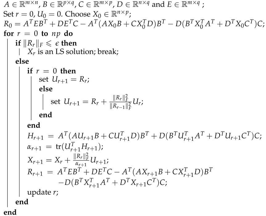Remark 1.

To terminate the algorithm, one can alternatively set the stopping rule to be ${\parallel R_r\parallel }_F-\delta ⩽{ϵ}^{\prime }$ where $\delta :=\parallel M{x}^{*}-e\parallel$ is the positive square root of the LS error described in Equation (16) and ${ϵ}^{\prime }>0$ is a small tolerance.

For any given initial matrix $X_0$, we will show that Algorithm 1 generates a sequence of approximate solutions $X_r$ of Equation (1), so that the set of residual matrices $R_r$ is orthogonal. It follows that a unique LS solution will be obtained within finite steps.

Lemma 7.

Assume that the sequences $\left\{R_r\right\}$ and $\left\{H_r\right\}$ are generated by Algorithm 1. We get

$$\begin{array}{c}\hfill R_{r+1}=R_r-\frac{{\parallel R_r\parallel }_F^2}{{\alpha }_{r+1}}{H}_{r+1},\mathit{for}r=1,2,\dots .\end{array}$$

(19)

Proof. 

From Algorithm 1, we have that for any r,

$$\begin{array}{cc}\hfill R_{r+1}& =A^{T}E{B}^T+D{E}^{T}C-A^T(A{X}_{r+1}B+C{X}_{r+1}^{T}D)B^T-D(B^T{X}_{r+1}^T{A}^T+D^T{X}_{r+1}{C}^T)C\hfill \\ \hfill & =A^{T}E{B}^T+D{E}^{T}C-A^T\left(A(X_r+\frac{{\parallel R_r\parallel }_F^2}{{\alpha }_{r+1}}{U}_{r+1})B+C{(X_r+\frac{{\parallel R_r\parallel }_F^2}{{\alpha }_{r+1}}{U}_{r+1})}^{T}D\right)B^T\hfill \\ \hfill & -D\left(B^T{(X_r+\frac{{\parallel R_r\parallel }_F^2}{{\alpha }_{r+1}}{U}_{r+1})}^T{A}^T+D^T(X_r+\frac{{\parallel R_r\parallel }_F^2}{{\alpha }_{r+1}}{U}_{r+1})C^T\right)C\hfill \\ \hfill & =A^{T}E{B}^T+D{E}^{T}C-A^T\left(A{X}_{r}B+\frac{{\parallel R_r\parallel }_F^2}{{\alpha }_{r+1}}A{U}_{r+1}B+C{X}_r^{T}D+\frac{{\parallel R_r\parallel }_F^2}{{\alpha }_{r+1}}C{U}_{r+1}^{T}D\right)B^T\hfill \\ \hfill & -D\left(B^T{X}_r^T{A}^T+\frac{{\parallel R_r\parallel }_F^2}{{\alpha }_{r+1}}{B}^T{U}_{r+1}^T{A}^T+D^T{X}_r{C}^T+\frac{{\parallel R_r\parallel }_F^2}{{\alpha }_{r+1}}{D}^T{U}_{r+1}{C}^T\right)C\hfill \\ \hfill & =A^{T}E{B}^T+D{E}^{T}C-A^T(A{X}_{r}B+C{X}_r^{T}D)B^T-D(B^T{X}_r^T{A}^T+D^T{X}_r{C}^T)C\hfill \\ \hfill & -\frac{{\parallel R_r\parallel }_F^2}{{\alpha }_{r+1}}[A^T(A{U}_{r+1}B+C{U}_{r+1}^{T}D)B^T+D(B^T{U}_{r+1}^T{A}^T+D^T{U}_{r+1}{C}^T)C]\hfill \\ \hfill & =R_r-\frac{{\parallel R_r\parallel }_F^2}{{\alpha }_{r+1}}{H}_{r+1}.\hfill \end{array}$$

   □

Lemma 8.

The sequences $\left\{U_r\right\}$ and $\left\{H_r\right\}$ generated by Algorithm 1 satisfy

$$\begin{array}{c}\hfill tr\left(U_m^T{H}_n\right)=tr\left(H_m^T{U}_n\right),\mathit{for}\mathit{any}m,n.\end{array}$$

(20)

Proof. 

Using the properties of the Kronecker product and the vector operator in Lemmas 1–5, we have

$$\begin{array}{cc}\hfill tr\left(H_m^T{U}_n\right)& ={(Vec{H}_m)}^{T}Vec{U}_n\hfill \\ \hfill & ={[Vec(A^T(A{U}_{m}B+C_j{U}_m^{T}D)B^T+D(B^T{U}_m^T{A}^T+D^T{U}_m{C}^T)C)]}^{T}Vec{U}_n\hfill \\ \hfill & ={[Vec\left(A^{T}A{U}_{m}B{B}^T\right)]}^{T}Vec{U}_n+{[Vec\left(A^{T}C{U}_m^{T}D{B}^T\right)]}^{T}Vec{U}_n\hfill \\ \hfill & +{[Vec\left(D{B}^T{U}_m^T{A}^{T}C\right)]}^{T}Vec{U}_n+{[Vec\left(D{D}^T{U}_m{C}^{T}C\right)]}^{T}Vec{U}_n\hfill \\ \hfill & ={(Vec{U}_m)}^T(B{B}^T\otimes A^{T}A)Vec{U}_n+{(Vec{U}_m^T)}^T(D{B}_k^T\otimes C^{T}A)Vec{U}_n\hfill \\ \hfill & +{(Vec{U}_m^T)}^T(A^{T}C\otimes B{D}^T)Vec{U}_n+{(Vec{U}_m)}^T(C^{T}C\otimes D{D}^T)Vec{U}_n\hfill \\ \hfill & =tr\left(B{B}^T{U}_m^T{A}^{T}A{U}_n\right)+tr\left(A^{T}C{U}_m^{T}D{B}^T{U}_n^T\right)+tr\left(D{B}^T{U}_m^T{A}^{T}C{U}_n^T\right)\hfill \\ \hfill & +tr\left(C^{T}C{U}_m^{T}D{D}^T{U}_n\right)\hfill \\ \hfill & ={(Vec\left(B{B}_k^T{U}_n^T{A}^{T}A\right))}^{T}Vec{U}_m^T+{(Vec\left(C^{T}A{U}_{n}B{D}^T\right))}^{T}Vec{U}_n^T\hfill \\ \hfill & +{(Vec\left(B{D}^T{U}_n{C}^{T}A\right))}^{T}Vec{U}_m^T+{(Vec\left(C^{T}C{U}_n^{T}D{D}^T\right))}^{T}Vec{U}_m^T\hfill \\ \hfill & ={[Vec\left(A^{T}A{U}_{n}B{B}^T\right)]}^{T}Vec{U}_m+{[Vec\left(D{B}^T{U}_n^T{A}^{T}C\right)]}^{T}Vec{U}_m\hfill \\ \hfill & +{[Vec\left(A^{T}C{U}_n^{T}D{B}^T\right)]}^{T}Vec{U}_m+{[Vec\left(D{D}^T{U}_n{C}^{T}C\right)]}^{T}Vec{U}_m\hfill \\ \hfill & ={[Vec(A^T(A{U}_{n}B+C{U}_n^{T}D)B^T+D(B^T{U}_n^T{A}^T+D^T{U}_n{C}^T)C)]}^{T}Vec{U}_m\hfill \\ \hfill & ={(Vec{H}_n)}^{T}Vec{U}_m\hfill \\ \hfill & =tr\left(H_n^T{U}_m\right)\hfill \\ \hfill & =tr\left(U_m^T{H}_n\right).\hfill \end{array}$$

   □

Lemma 9.

The sequences $\left\{R_r\right\}$, $\left\{U_r\right\}$ and $\left\{H_r\right\}$ generated by Algorithm 1 satisfy

$$tr\left(R_r^T{R}_{r-1}\right)=0,\mathit{and}tr\left(U_{r+1}^T{H}_r\right)=0,\mathit{forany}r.$$

(21)

Proof. 

We use the induction principle to prove (21). In order to calculate related terms, we utilize Lemmas 7 and 8. For $r=1,$ we get

$$\begin{array}{cc}\hfill tr\left(R_1^T{R}_0\right)& =tr\left(R_0^T{R}_0\right)-\frac{{\parallel R_0\parallel }_F^2}{{\alpha }_1}tr\left(H_1^T{R}_0\right)=0,\hfill \\ \hfill tr\left(U_2^T{H}_1\right)& =tr\left(R_1^T{H}_1\right)+\frac{{\parallel R_1\parallel }_F^2}{{\parallel R_0\parallel }_F^2}tr\left(U_1^T{H}_1\right)\hfill \\ \hfill & =-\frac{{\alpha }_1}{{\parallel R_0\parallel }_F^2}tr\left(R_1^T{R}_1\right)+{\alpha }_1\frac{{\parallel R_1\parallel }_F^2}{{\parallel R_0\parallel }_F^2}=0.\hfill \end{array}$$

These imply that (21) holds for $r=1$. Now, we proceed the inductive step by assuming that $tr\left(R_r^T{R}_{r-1}\right)=0$ and $tr\left(U_{r+1}^T{H}_r\right)=0$. Then

$$\begin{array}{cc}\hfill tr\left(R_{r+1}^T{R}_r\right)& =tr\left(R_r^T{R}_r\right)-\frac{{\parallel R_r\parallel }_F^2}{{\alpha }_{r+1}}tr\left(H_{r+1}^T\left(U_{r+1}-\frac{{\parallel R_r\parallel }_F^2}{{\parallel R_{r-1}\parallel }_F^2}{U}_r\right)\right)\hfill \\ \hfill & ={\parallel R_r\parallel }_F^2-\frac{{\parallel R_r\parallel }_F^2}{{\alpha }_{r+1}}tr\left(H_{r+1}^T{U}_{r+1}\right)=0,\hfill \\ \hfill tr\left(U_{r+2}^T{H}_{r+1}\right)& =tr\left(R_{r+1}^T\left(\frac{-{\alpha }_{r+1}}{{\parallel R_r\parallel }_F^2}(R_{r+1}-R_r)\right)\right)+\frac{{\parallel R_{r+1}\parallel }_F^2}{{\parallel R_r\parallel }_F^2}{\alpha }_{r+1}\hfill \\ \hfill & =\frac{{\alpha }_{r+1}}{{\parallel R_r\parallel }_F^2}tr[\left(R_{r+1}^T{R}_r\right)-\left(R_{r+1}^T{R}_{r+1}\right)]+\frac{{\parallel R_{r+1}\parallel }_F^2}{{\parallel R_r\parallel }_F^2}{\alpha }_{r+1}=0.\hfill \end{array}$$

Hence, Equationd (21) holds for any r.    □

Lemma 10.

Suppose the sequences $\left\{R_r\right\}$, $\left\{U_r\right\}$ and $\left\{H_r\right\}$ are constructed from Algorithm 1. Then

$$\begin{array}{c}\hfill tr\left(R_r^T{R}_0\right)=0,tr\left(U_{r+1}^T{H}_1\right)=0,\mathit{for}\mathit{any}r.\end{array}$$

(22)

Proof. 

The initial step $r=1$ holds due to Lemma 9. Now, assume that Equation (22) is valid for all $r=1,\dots ,k$. From Lemmas 7 and 8, we get

$$\begin{array}{cc}\hfill tr\left(R_{k+1}^T{R}_0\right)& =tr\left({\left(R_k-\frac{{\parallel R_k\parallel }_F^2}{{\alpha }_{k+1}}{V}_{k+1}\right)}^T{R}_0\right)=tr\left(R_k^T{R}_0\right)-\frac{{\parallel R_k\parallel }_F^2}{{\alpha }_{k+1}}tr\left(H_{k+1}^T{R}_0\right)\hfill \\ \hfill & =-\frac{{\parallel R_k\parallel }_F^2}{{\alpha }_{k+1}}tr\left(H_{k+1}^T{U}_1\right)=-\frac{{\parallel R_k\parallel }_F^2}{{\alpha }_{k+1}}tr\left(U_{k+1}^T{H}_1\right)=0,\hfill \end{array}$$

and

$$\begin{array}{cc}\hfill tr\left(U_{k+2}^T{H}_1\right)& =tr\left(H_{k+2}^T{U}_1\right)=tr\left({\left(\frac{-{\alpha }_{k+2}}{{\parallel R_{k+1}\parallel }_F^2}\left(R_{k+2}-R_{k+1}\right)\right)}^T{U}_1\right)\hfill \\ \hfill & =\frac{-{\alpha }_{k+2}}{{\parallel R_{k+1}\parallel }_F^2}[tr\left(R_{k+2}^T{R}_0\right)-tr\left(R_{k+1}^T{R}_0\right)]=0.\hfill \end{array}$$

Hence, Equation (22) holds for any r.    □

Lemma 11.

Suppose the sequences $\left\{R_r\right\}$, $\left\{U_r\right\}$ and $\left\{H_r\right\}$ are constructed from Algorithm 1. Then for any integers m and n such that $m\ne n$, we have

$$\begin{array}{c}\hfill tr\left(R_{m-1}^T{R}_{n-1}\right)=0,\mathrm{and}tr\left(U_m^T{H}_n\right)=0.\end{array}$$

(23)

Proof. 

According to Lemma 8 and the fact that $tr\left(R_{m-1}^T{R}_{n-1}\right)=tr\left(R_{n-1}^T{R}_{m-1}\right)$ for any integers m and n, it remains to prove two equalities in (23) for only $m,n$ such that $m>n$. For $m=n+1$, the two equalities hold by Lemma 9. For $m=n+2$, we have

$$\begin{array}{cc}\hfill tr\left(R_{n+2}^T{R}_n\right)& =tr\left({\left(R_{n+1}-\frac{{\parallel R_{n+1}\parallel }_F^2}{{\alpha }_{n+2}}{H}_{n+2}\right)}^T{R}_n\right)\hfill \\ \hfill & =-\frac{{\parallel R_{n+1}\parallel }_F^2}{{\alpha }_{n+2}}tr\left(H_{n+2}^T\left(U_{n+1}-\frac{{\parallel R_n\parallel }_F^2}{{\parallel R_{n-1}\parallel }_F^2}{U}_n\right)\right)\hfill \\ \hfill & =\frac{{\parallel R_{n+1}\parallel }_F^2}{{\alpha }_{n+2}}\frac{{\parallel R_n\parallel }_F^2}{{\parallel R_{n-1}\parallel }_F^2}tr\left({\left(R_{n+1}+\frac{{\parallel R_{n+1}\parallel }_F^2}{{\parallel R_n\parallel }_F^2}{U}_{n+1}\right)}^T{H}_n\right)\hfill \\ \hfill & =\frac{{\parallel R_{n+1}\parallel }_F^2}{{\alpha }_{n+2}}\frac{{\parallel R_n\parallel }_F^2}{{\parallel R_{n-1}\parallel }_F^2}\frac{{\alpha }_n}{{\parallel R_{n-1}\parallel }_F^2}tr\left(R_{n+1}^T{R}_{n-1}\right),\hfill \end{array}$$

and, similarly, we have

$$\begin{array}{cc}\hfill tr\left(R_{n+1}^T{R}_{n-1}\right)& =\frac{{\parallel R_n\parallel }_F^2}{{\alpha }_{n+1}}\frac{{\parallel R_{n-1}\parallel }_F^2}{{\parallel R_{n-2}\parallel }_F^2}\frac{{\alpha }_{n-1}}{{\parallel R_{n-2}\parallel }_F^2}tr\left(R_n^T{R}_{n-2}\right),\hfill \\ \hfill tr\left(R_n^T{R}_{n-2}\right)& =\frac{{\parallel R_{n-1}\parallel }_F^2}{{\alpha }_n}\frac{{\parallel R_{n-2}\parallel }_F^2}{{\parallel R_{n-3}\parallel }_F^2}\frac{{\alpha }_{n-2}}{{\parallel R_{n-3}\parallel }_F^2}tr\left(R_{n-1}^T{R}_{n-3}\right).\hfill \end{array}$$

Moreover,

$$\begin{array}{cc}\hfill tr\left(U_{n+2}^T{H}_n\right)& =tr\left({\left(R_{n+1}-\frac{{\parallel R_{n+1}\parallel }_F^2}{{\parallel R_n\parallel }_F^2}{U}_{n+1}\right)}^T{H}_n\right)\hfill \\ \hfill & =tr\left(R_{n+1}^T\left(\frac{-{\alpha }_n}{{\parallel R_{n-1}\parallel }_F^2}\left(R_n-R_{n-1}\right)\right)\right)\hfill \\ \hfill & =\frac{{\alpha }_n}{{\parallel R_{n-1}\parallel }_F^2}tr\left({\left(R_n-\frac{{\parallel R_n\parallel }_F^2}{{\alpha }_{n+1}}{H}_{n+1}\right)}^T{R}_{n-1}\right)\hfill \\ \hfill & =-\frac{{\alpha }_n}{{\parallel R_{n-1}\parallel }_F^2}\frac{{\parallel R_n\parallel }_F^2}{{\alpha }_{n+1}}\left[tr\left(H_{n+1}^T{U}_n\right)-\frac{{\parallel R_{n-1}\parallel }_F^2}{{\parallel R_{n-2}\parallel }_F^2}tr\left(H_{n+1}^T{U}_{n-1}\right)\right]\hfill \\ \hfill & =\frac{{\alpha }_n}{{\parallel R_{n-1}\parallel }_F^2}\frac{{\parallel R_n\parallel }_F^2}{{\alpha }_{n+1}}\frac{{\parallel R_{n-1}\parallel }_F^2}{{\parallel R_{n-2}\parallel }_F^2}tr\left(U_{n+1}^T{H}_{n-1}\right),\hfill \end{array}$$

and, similarly,

$$\begin{array}{cc}\hfill tr\left(U_{n+1}^T{H}_{n-1}\right)& =\frac{{\alpha }_{n-1}}{{\parallel R_{n-2}\parallel }_F^2}\frac{{\parallel R_{n-1}\parallel }_F^2}{{\alpha }_n}\frac{{\parallel R_{n-2}\parallel }_F^2}{{\parallel R_{n-3}\parallel }_F^2}tr\left(U_n^T{H}_{n-2}\right).\hfill \end{array}$$

In a similar way, we can write $tr\left(R_{n+1}^T{R}_{n-1}\right)$ and $tr\left(U_{n+2}^T{H}_n\right)$ in terms of $tr\left(R_n^T{R}_{n-2}\right)$ and $tr\left(U_{n+1}^T{H}_{n-1}\right)$, respectively. Continuing this process until the terms $tr\left(R_2^T{R}_0\right)$ and $tr\left(U_3^T{H}_1\right)$ appear. By Lemma 10, we get $tr\left(R_{n+1}^T{R}_{n-1}\right)=0$ and $tr\left(U_{n+2}^T{H}_n\right)=0$. Similarly, we have $tr\left(R_m^T{R}_{n-1}\right)=0$ and $tr\left(U_m^T{H}_n\right)=0$ for $m=n+3,\dots ,k$.

Suppose that $tr\left(R_{m-1}^T{R}_{n-1}\right)=tr\left(U_m^T{H}_n\right)=0$ for $m\in \{n+1,\dots ,k\}$. Then for $m=k+1$, we have

$$\begin{array}{cc}\hfill tr\left(R_k^T{R}_{n-1}\right)& =tr\left(R_{k-1}^T{R}_{n-1}\right)-\frac{{\parallel R_{k-1}\parallel }_F^2}{{\alpha }_k}tr\left(H_k^T{R}_{n-1}\right)\hfill \\ \hfill & =-\frac{{\parallel R_{k-1}\parallel }_F^2}{{\alpha }_k}tr\left(H_k^T\left(U_n-\frac{{\parallel R_{n-1}\parallel }_F^2}{{\parallel R_{n-2}\parallel }_F^2}{U}_{n-1}\right)\right)\hfill \\ \hfill & =-\frac{{\parallel R_{k-1}\parallel }_F^2}{{\alpha }_k}\left[tr\left(H_k^T{U}_n\right)-\frac{{\parallel R_{n-1}\parallel }_F^2}{{\parallel R_{n-2}\parallel }_F^2}tr\left(H_k^T{U}_{n-1}\right)\right]=0.\hfill \end{array}$$

and

$$\begin{array}{cc}\hfill tr\left(U_{k+1}^T{H}_n\right)& =tr\left(R_k^T{H}_n\right)+\frac{{\parallel R_k\parallel }_F^2}{{\parallel R_{k-1}\parallel }_F^2}tr\left(U_k^T{H}_n\right)=tr\left(R_k^T\left(\frac{-{\alpha }_n}{{\parallel R_{n-1}\parallel }_F^2}\left(R_n-R_{n-1}\right)\right)\right)\hfill \\ \hfill & =\frac{-{\alpha }_n}{{\parallel R_{n-1}\parallel }_F^2}tr(R_k^T{R}_n-R_k^T{R}_{n-1})=0.\hfill \end{array}$$

Hence, $tr\left(R_{m-1}^T{R}_{n-1}\right)=0$ and $tr\left(U_m^T{H}_n\right)=0$ for any $m,n$ such that $m\ne n$.    □

Theorem 1.

Algorithm 1 solves Problem 1 within finite steps. More precisely, for any given initial matrix $X_0\in {\mathbb{R}}^{n\times p}$, the sequence $\left\{X_r\right\}$ constructed from Algorithm 1 converges to an LS solution of Equation (1) in at most $np$ iterations.

Proof. 

Assume that $R_r\ne 0$ for $r=0,1,\dots ,np-1$. Assume that $R_{np}\ne 0$. By Lemma 11, the set $\{R_0,R_1,\dots ,R_{np}\}$ of residual matrices is orthogonal in ${\mathbb{R}}^{n\times p}$ with respect to the Frobenius inner product (5). Therefore, the set $\{R_0,R_1,\dots ,R_{np}\}$ of $np+1$ elements is linearly independent. This contradicts the fact that the dimension of ${\mathbb{R}}^{n\times p}$ is $np$. Thus, $R_{np}=0$, and $X_{np}$ satisfies Equation (15) in Lemma 6. Hence $X_{np}$ is an LS solution of Equation (1).    □

We adapt the same idea as that for Algorithm 1 to derive an algorithm for Equation (2) as follows:

Algorithm 2: A conjugate gradient iterative algorithm for Equation (2)

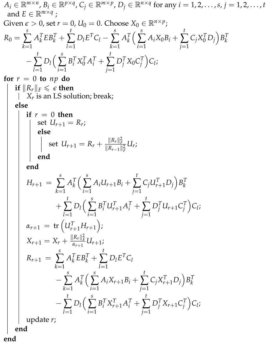The stopping rule of Algorithm 2 may be described as ${\parallel R_r\parallel }_F-\delta ⩽{ϵ}^{\prime }$ where $\delta$ is the positive square root of the associated LS error and ${ϵ}^{\prime }>0$ is a small tolerance.

Theorem 2.

Consider Equation (2) where $A_i\in {\mathbb{R}}^{m\times n}$, $B_i\in {\mathbb{R}}^{p\times q}$, $C_j\in {\mathbb{R}}^{m\times p}$, $D_j\in {\mathbb{R}}^{n\times q}$, $D\in {\mathbb{R}}^{m\times q}$, $E\in {\mathbb{R}}^{m\times q}$ are given constant matrices and $X\in {\mathbb{R}}^{n\times p}$ is an unknown matrix. Assume that the matrix

$$\begin{array}{c}\hfill M:=\sum _{i=1}^s(B_i^T\otimes A_i)+\sum _{j=1}^t(D_j^T\otimes C_j)P(n,p)\end{array}$$

(24)

is of full-column rank. Then, for any given initial matrix $X_0\in {\mathbb{R}}^{n\times p}$, the sequence $\left\{X_r\right\}$ constructed from Algorithm 2 converges to a unique LS solution.

Proof. 

The proof of is similar to that of Theorem 1.   □

5. Minimal-Norm Least-Squares Solution via Algorithm 1

In this section, we investigate Problem 2. That is, we consider the case when the matrix M may not have full-column rank, so that Equation (1) may have many LS solutions. We shall seek for an element of $\mathcal{L}$ with the minimal Frobenius norm.

Lemma 12.

Assume $\widehat{X}\in \mathcal{L}$. Then, any arbitrary element $\tilde{X}\in \mathcal{L}$ can be expressed as $\widehat{X}+Z$ for some matrix $Z\in {\mathbb{R}}^{n\times p}$ satisfying

$$\begin{array}{c}\hfill A^T(AZB+C{Z}^{T}D)B^T+D(B^T{Z}^T{A}^T+D^{T}Z{C}^T)C=0.\end{array}$$

(25)

Proof. 

Let us denote the residual of the LS solutions $\widehat{X}$ and $\tilde{X}$, according to Equation (18), by $R_{\widehat{X}}$ and $R_{\tilde{X}}$, respectively. We consider the different $Z:=\tilde{X}-\widehat{X}$. Now, we compute

$$\begin{array}{cc}\hfill R_{\tilde{X}}& =A^T(A(\widehat{X}+Z)B+C{(\widehat{X}+Z)}^{T}D)B^T+D(B^T{(\widehat{X}+Z)}^T{A}^T+D^T(\widehat{X}+Z)C^T)C\hfill \\ \hfill & -A^{T}E{B}^T-D{E}^{T}C\hfill \\ \hfill & =A^T(AZB+C{Z}^{T}D)B^T+D(B^T{Z}^T{A}^T+D^{T}Z{C}^T)C-R_{\widehat{X}}.\hfill \end{array}$$

Since $\widehat{X},\tilde{X}\in \mathcal{L}$, by Lemma 6 we have $R_{\widehat{X}}=R_{\tilde{X}}=0$. It follows that Equation (25) holds as desired.   □

Theorem 3.

Algorithm 1 solves Problem 2 in at most $np$ iterations by starting with the initial matrix

$$\begin{array}{c}\hfill X_0=A^T(A{V}_{0}B+C{V}_0^{T}D)B^T+D(B^T{V}_0^T{A}^T+D^T{V}_0{C}^T)C,\end{array}$$

(26)

where $V_0\in {\mathbb{R}}^{n\times p}$ is an arbitrary matrix, or especially $X_0=0$.

Proof. 

If we run Algorithm 1 starting with (26), then we can write the solution $X^{*}$ of Problem 2 so that

$$X^{*}=A^T(A{V}^{*}B+C{V}^{*T}D)B^T+D(B^T{V}^{*T}{A}^T+D^T{V}^{*}{C}^T)C,$$

for some matrix $V^{*}\in {\mathbb{R}}^{n\times p}$. Now, assume that $\tilde{X}$ is an arbitrary element in $\mathcal{L}$. By Lemma 12, there is a matrix $Z\in {\mathbb{R}}^{n\times p}$ such that $\tilde{X}=X^{*}+Z$ and

$$A^T(AZB+C{Z}^{T}D)B^T+D(B^T{Z}^T{A}^T+D^{T}Z{C}^T)C=0.$$

Using the property (6), we get

$$\begin{array}{cc}\hfill ⟨X^{*},Z⟩& =⟨A^T(A{V}^{*}B+C{V}^{*T}D)B^T+D(B^T{V}^{*T}{A}^T+D^T{V}^{*}{C}^T)C,Z⟩\hfill \\ \hfill & =⟨V^{*},A^T(AZB+C{Z}^{T}D)B^T+D(B^T{Z}^T{A}^T+D^{T}Z{C}^T)C⟩\hfill \\ \hfill & =0.\hfill \end{array}$$

Since $X^{*}$ is orthogonal to Z, it follows from the Pythagorean theorem that

$$\begin{array}{c}\hfill {\parallel \tilde{X}\parallel }_F^2={\parallel X^{*}+Z\parallel }_F^2={\parallel X^{*}\parallel }_F^2+{\parallel Z\parallel }_F^2\ge {\parallel X^{*}\parallel }_F^2.\end{array}$$

This implies that $X^{*}$ is the minimal-norm solution.   □

Theorem 4.

Consider the sequence $\left\{X_r\right\}$ generated by Algorithm 2 starting with the initial matrix

$$\begin{array}{c}\hfill {\displaystyle X_0=\sum _{k=1}^s{A}_k^T\left({\displaystyle \sum _{i=1}^s{A}_i{V}_0{B}_i+\sum _{j=1}^t{C}_j{V}_0^T{D}_j}\right)B_k^T+\sum _{l=1}^t{D}_l\left({\displaystyle \sum _{i=1}^s{B}_i^T{V}_0^T{A}_i^T+\sum _{j=1}^t{D}_j^T{V}_0{C}_j^T}\right)C_l,}\end{array}$$

where $V_0\in {\mathbb{R}}^{n\times p}$ is an arbitrary matrix, or especially $X_0=0\in {\mathbb{R}}^{n\times p}$. Then the sequence $\left\{X_r\right\}$ converges to the minimal-norm LS solution of Equatiom (2) in at most $np$ iterations.

Proof. 

The proof is similar to that of Theorem 3.   □

6. Least-Squares Solution Closest to a Given Matrix

In this section, we investigate Problem 3. In this case, Equation (1) may have many LS solutions. We shall seek for one that closest to a given matrix with respect to the Frobenius norm.

Theorem 5.

Algorithm 1 solves Problem 3 by substituting E with $E_1=E-(AYB+C{Y}^{T}D)$, and choosing the initial matrix to be

$$\begin{array}{c}\hfill W_0=A^T(AVB+C{V}^{T}D)B^T+D(B^T{V}^T{A}^T+D^{T}V{C}^T)C,\end{array}$$

(27)

where $V\in {\mathbb{R}}^{n\times p}$ is arbitrary, or specially $W_0=0\in {\mathbb{R}}^{n\times p}$.

Proof. 

Let $Y\in {\mathbb{R}}^{n\times p}$ be given. We can translate Problem 3 into Problem 2 as follows:

$$\begin{array}{cc}\hfill \underset{X\in {\mathbb{R}}^{n\times p}}{min}& {\parallel AXB+C{X}^{T}D-E\parallel }_F\hfill \\ \hfill & =\underset{X\in {\mathbb{R}}^{n\times p}}{min}{\parallel AXB+C{X}^{T}D-E-AYB-C{Y}^{T}D+AYB+C{Y}^{T}D\parallel }_F\hfill \\ \hfill & =\underset{X\in {\mathbb{R}}^{n\times p}}{min}{\parallel A(X-Y)B+C{(X-Y)}^{T}D-E+AYB+C{Y}^{T}D\parallel }_F.\hfill \end{array}$$

Now, substituting $E_1=E-(AYB+C{Y}^{T}D)$ and $W=X-Y$, we see that the solution $\check{X}$ of Problem 3 is equal to $W^{*}+Y$ where $W^{*}$ is the minimal-norm LS solution of the equation

$$\begin{array}{c}\hfill AWB+C{W}^{T}D=E_1,\end{array}$$

in unknown W. By Theorem 3, the matrix $W^{*}$ can be solved by Algorithm 1 with the initial matrix (27) where $V\in {\mathbb{R}}^{n\times p}$ is arbitrary matrix, or especially $W_0=0$.   □

Theorem 6.

Suppose that the matrix Equation (2) is inconsistent. Let $Y\in {\mathbb{R}}^{n\times p}$ be given. Consider Algorithm 2 when we replace the matrix E by

$$\begin{array}{c}\hfill E_1=E-\sum _{i=1}^s{A}_{i}Y{B}_i-\sum _{j=1}^t{C}_j{Y}^T{D}_j,\end{array}$$

and choose the initial matrix

$$\begin{array}{c}\hfill {\displaystyle W_0=\sum _{k=1}^s{A}_k^T\left({\displaystyle \sum _{i=1}^s{A}_{i}F{B}_i+\sum _{j=1}^t{C}_j{F}^T{D}_j}\right)B_k^T+\sum _{l=1}^t{D}_l\left({\displaystyle \sum _{i=1}^s{B}_i^T{F}^T{A}_i^T+\sum _{j=1}^t{D}_j^{T}F{C}_j^T}\right)C_l,}\end{array}$$

where $F\in {\mathbb{R}}^{n\times p}$ is arbitrary, or $W_0=0\in {\mathbb{R}}^{n\times p}$. Then, the sequence $\left\{X_r\right\}$ obtained by Algorithm 2 converges to the LS solution of (2) closest to Y within $np$ iterations.

Proof. 

The proof of the theorem is similar to that of Theorem 5.   □

7. Numerical Experiments

In this section, we provide numerical results to show the efficiency and effectiveness of Algorithm 2 (denoted by CG), which is an extension of Algorithm 1. We perform experiments when the coefficients in a given matrix equation are dense/sparse rectangular matrices of moderate/large sizes. We denote by $ones(m,n)$ the m-by-n matrix whose all entries are 1. Each random matrix $rand(m,n)$ has all entries belonging to the interval $(0,1)$. Each experiment contains some comparisons of Algorithm 2 with the direct Kronecker linearization as well as well-known iterative algorithms. All iterations were performed by MATLAB R2021a, on Mac operating system (M1 chip 8C CPU/8C GPU/8GB/512GB). The performance of algorithms is investigated through the number of iterations, the norm of residual matrices, and the CPU time. The latter is measured in seconds using the functions $tic$ and $toc$ on MATLAB.

The next is an example of Problem 1.

Example 1.

Consider a generalized Sylvester-transpose matrix equation

$$\begin{array}{c}\hfill A_{1}X{B}_1+A_{2}X{B}_2+A_{3}X{B}_3+C_1{X}^T{D}_1+C_2{X}^T{D}_2=E,\end{array}$$

(28)

where the coefficient matrices are given by

$$\begin{array}{cccc}\hfill & A_1=0.5ones(m,n)-rand(m,n)\in {\mathbb{R}}^{50\times 50},\hfill & \hfill & A_2=0.5ones(m,n)-rand(m,n)\in {\mathbb{R}}^{50\times 50},\hfill \\ \hfill & A_3=0.5ones(m,n)-rand(m,n)\in {\mathbb{R}}^{50\times 50},\hfill & \hfill & B_1=0.5ones(p,q)-rand(p,q)\in {\mathbb{R}}^{40\times 50},\hfill \\ \hfill & B_2=0.5ones(p,q)-rand(p,q)\in {\mathbb{R}}^{40\times 50},\hfill & \hfill & B_3=0.5ones(p,q)-rand(p,q)\in {\mathbb{R}}^{40\times 50},\hfill \\ \hfill & C_1=0.5ones(m,p)-rand(m,p)\in {\mathbb{R}}^{50\times 40},\hfill & \hfill & C_2=0.5ones(m,p)-rand(m,p)\in {\mathbb{R}}^{50\times 40},\hfill \\ \hfill & D_1=0.5ones(n,q)-rand(n,q)\in {\mathbb{R}}^{50\times 50},\hfill & \hfill & D_2=0.5ones(n,q)-rand(n,q)\in {\mathbb{R}}^{50\times 50},\hfill \\ \hfill & E=0.5ones(m,q)-rand(m,q)\in {\mathbb{R}}^{50\times 50}.\hfill \end{array}$$

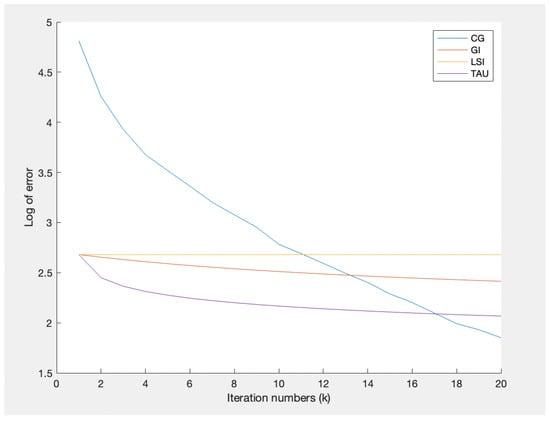
In fact, we have $rankM=2000\ne 2001=rank\left[Me\right]$, i.e., the matrix equation does not have an exact solution. However, M is of full-column rank, so this equation has a unique LS solution. We run Algorithm 2 using an initial matrix $X_0=0\in {\mathbb{R}}^{50\times 40}$ and a tolerance error $ϵ=\parallel M{x}^{*}-e\parallel =6.4812$, where $x^{*}={\left(M^{T}M\right)}^{-1}{M}^{T}e$. It turns out that Algorithm 2 takes 20 iterations to get a least-square solution, consuming around $0.2$ s, while the direct method consumes around 7 s. Thus, Algorithm 2 takes 35 times less computational time than the direct method. We compare the performance of Algorithm 2 with other well-known iterative algorithms: GI method [31], LSI method [31], and TAUOpt method [32]. The numerical results are shown in Table 1 and Figure 1. We see that after running 20 iterations, Algorithm 2 consumes CTs slightly more than other methods, but the relative error ${\parallel R_r\parallel }_F$ is less than those of the others. Hence, Algorithm 2 is applicable and has a good performance.

Table 1. Relative error and computational time for Example 1.

Method	Iterations	CPU	${\parallel {\mathit{R}}_{\mathit{r}}\parallel }_{\mathit{F}}$
CG	20	0.199308	6.407766
GI	20	0.129715	10.907665
LSI	20	0.179449	14.390460
TAUOpt	20	0.073866	7.806273
Direct	−	7.048632	0

Figure 1. The logarithm of the relative error ${\parallel R_r\parallel }_F$ for Example 1.

The next is an example of Problem 2.

Example 2.

Consider a generalized Sylvester-transpose matrix equation

$$\begin{array}{c}\hfill A_{1}X{B}_1+C_1{X}^T{D}_1+C_2{X}^T{D}_2=E,\end{array}$$

(29)

where

$$\begin{array}{cccc}\hfill & A_1=-0.08\times ones(m,n)\in {\mathbb{R}}^{30\times 25},\hfill & \hfill & B_1=tridiag(0.11,-0.61,-0.29)\in {\mathbb{R}}^{30\times 30},\hfill \\ \hfill & C_1=tridiag(-0.03,-0.22,-0.1)\in {\mathbb{R}}^{30\times 30},\hfill & \hfill & C_2=tridiag(0.38,0.29,-0.41)\in {\mathbb{R}}^{30\times 30},\hfill \\ \hfill & D_1=-0.13\times ones(n,q)\in {\mathbb{R}}^{25\times 30},\hfill & \hfill & D_2=0.04\times ones(n,q)\in {\mathbb{R}}^{25\times 30},\hfill \\ \hfill & E=-0.01\times I_{30}\in {\mathbb{R}}^{30\times 30}.\hfill \end{array}$$

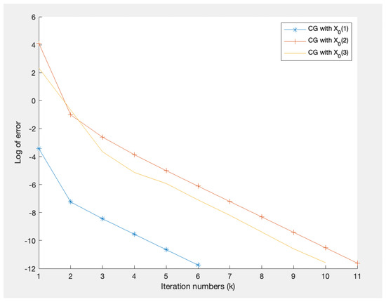
In this case, Equation (29) is inconsistent and the associated matrix M is not of full-column rank. Thus, Equation (29) has many LS solutions. The direct method concerning Moore–Penrose inverse (17) takes $0.627019$ s to get the minimal-norm LS solutions. Alternatively, MNLS method [35] can be also used to this kind of problem. However, some coefficient matrices are triangular matrices with multiple zeros, causing the MNLS algorithm diverges and cannot provide answer. Therefore, let us apply Algorithm 2 using a tolerance error $ϵ={10}^{-5}$. According to Theorem 4, we choose three different matrices $V_0$ to generate the initial matrix $X_0$. The numerical results are shown in Table 2 and Figure 2.

Table 2. Relative error and computational time for Example 2.

${\mathit{V}}_0$	Iterations	CPU	${\parallel {\mathit{R}}_{\mathit{r}}\parallel }_{\mathit{F}}$
0	6	0.036523	0.000008
0.02 × ones	11	0.036540	0.000009
−0.01 $\times I$	10	0.038425	0.000009

Figure 2. The logarithm of the relative error for Example 2.

Figure 2 shows that the logarithm of the relative errors ${\parallel R_r\parallel }_F$ for CG algorithms, using three initial matrices, are rapidly decreasing to zero. All of them consume around $0.037$ s to arrive at the desired solution, which is 16 times less than the direct method.

The following is an example of Problem 3.

Example 3.

Consider a generalized Sylvester-transpose matrix equation

$$\begin{array}{c}\hfill A_{1}X{B}_1+C_1{X}^T{D}_1+C_2{X}^T{D}_2=E,\end{array}$$

(30)

where

$$\begin{array}{cccc}\hfill & A_1=0.2\times ones(m,n)\in {\mathbb{R}}^{50\times 40},\hfill & \hfill & B_1=tridiag(-0.2,0.3,0.3)\in {\mathbb{R}}^{50\times 50},\hfill \\ \hfill & C_1=tridiag(0.4,-0.2,-0.1)\in {\mathbb{R}}^{50\times 50},\hfill & \hfill & C_2=tridiag(0.7,-0.2,0.3)\in {\mathbb{R}}^{50\times 50},\hfill \\ \hfill & D_1=-0.2\times ones(n,q)\in {\mathbb{R}}^{40\times 50},\hfill & \hfill & D_2=0.1\times ones(n,q)\in {\mathbb{R}}^{40\times 50},\hfill \\ \hfill & E=I_{50}\in {\mathbb{R}}^{50\times 50}.\hfill \end{array}$$

In fact, Equation (30) is inconsistent and has many LS solutions. The first task is to find the LS solution of Equation (30) closest to $Y=0.1\times ones(n,p)\in {\mathbb{R}}^{40\times 50}$. According to Theorem 6, we apply Algorithm 2 with two different matrices V to construct the initial matrix $W_0$. Algorithm 2 with $V=0$ and $V=-0.19\times I$ are denoted in Figure 3 by $C{G}_1$ and $C{G}_2$, respectively.

The second task is to solve Problem 3 when we are given $Y=0.1\times ones(n,p)\in {\mathbb{R}}^{40\times 50}$. Similarly, we use two different matrices $V=0$ and $V=0.02\times ones(n,p)\in {\mathbb{R}}^{40\times 50}$ to construct the initial matrix.

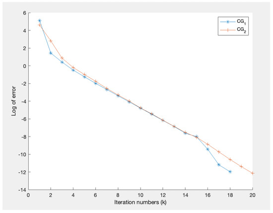
Figure 3. The logarithm of the relative error for Example 3 with Y = 0.1 $\times ones(n,p)$.

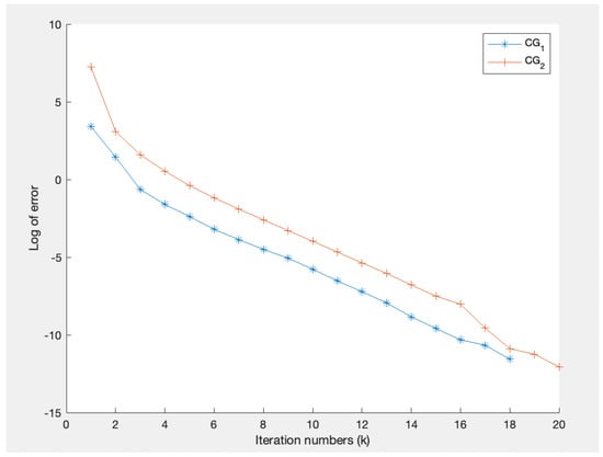
Figure 4. The logarithm of the relative error for Example 3 with Y = I.

Table 3. Relative error and computational time for Example 3.

Y	Initial V	Iterations	CPU	${\parallel {\mathit{R}}_{\mathit{r}}\parallel }_{\mathit{F}}$	${\parallel {\mathit{X}}^{*}-\mathit{Y}\parallel }_{\mathit{F}}$
$0.1\times ones(n,p)$	0	18	0.104135	0.000006	4.3116
	$-0.19\times I$	20	0.108153	0.000005	4.3116
I	0	18	0.113960	0.000009	0.8580
	$0.02\times ones$	20	0.108499	0.000006	0.8580

Table 3. Relative error and computational time for Example 3.

Y	Initial V	Iterations	CPU	${\parallel {\mathit{R}}_{\mathit{r}}\parallel }_{\mathit{F}}$	${\parallel {\mathit{X}}^{*}-\mathit{Y}\parallel }_{\mathit{F}}$
$0.1\times ones(n,p)$	0	18	0.104135	0.000006	4.3116
	$-0.19\times I$	20	0.108153	0.000005	4.3116
I	0	18	0.113960	0.000009	0.8580
	$0.02\times ones$	20	0.108499	0.000006	0.8580

We apply Algorithm 2 with a tolerance error $ϵ={10}^{-5}$. The numerical results in Figure 3 and Figure 4, and Table 3 illustrate that, in each case, the relative error converges rapidly to zero within 20 iterations, consuming around $0.1$ s. Thus, Algorithm 2 performs well in both the number of iterations and computational time. Moreover, changing initial matrix and the desired matrix Y does not siginificantly affect the performance of algorithm.

8. Conclusions

We propose CG-type iterative algorithms, namely, Algorithms 1 and 2, to generate approximate solutions for the generalized Sylvester-transpose matrix Equations (1) and (2), respectively. When the matrix equation is inconsistent, the algorithm will arrive at an LS solution within $np$ iterations with the absence of round-off errors. When the matrix equation has many LS solutions, the algorithm can search for the one with minimal Frobenius norm within $np$ steps. Moreover, given a matrix Y, the algorithm can find the LS solution closest to Y within $np$ steps. The numerical simulations validate the relevance of the algorithm for medium/large sizes of squares/non-squares matrices. The algorithm is always applicable for any given initial matrix and the given matrix Y. The algorithm performs well in both the number of iterations and computational times, compared to the direct Kronecker linearization and well-known iterative methods.

References

- Geir, E.D.; Fernando, P. A Course in Robust Control Theory: A Convex Approach; Springer: New York, NY, USA, 1999. [Google Scholar]
- Lewis, F. A survey of linear singular systems. Circ. Syst. Signal Process. 1986, 5, 3–36. [Google Scholar] [CrossRef]
- Dai, L. Singular Control Systems; Springer: Berlin, Germany, 1989. [Google Scholar]
- Enright, W.H. Improving the efficiency of matrix operations in the numerical solution of stiff ordinary differential equations. ACM Trans. Math. Softw. 1978, 4, 127–136. [Google Scholar] [CrossRef]
- Aliev, F.A.; Larin, V.B. Optimization of Linear Control Systems: Analytical Methods and Computational Algorithms; Stability Control Theory, Methods Applications; CRC Press: Boca Raton, FL, USA, 1998. [Google Scholar]
- Calvetti, D.; Reichel, L. Application of ADI iterative methods to the restoration of noisy images. SIAM J. Matrix Anal. Appl. 1996, 17, 165–186. [Google Scholar] [CrossRef]
- Duan, G.R. Eigenstructure assignment in descriptor systems via output feedback: A new complete parametric approach. Int. J. Control 1999, 72, 345–364. [Google Scholar] [CrossRef]
- Duan, G.R. Parametric approaches for eigenstructure assignment in high-order linear systems. Int. J. Control Autom. Syst. 2005, 3, 419–429. [Google Scholar]
- Kim, Y.; Kim, H.S. Eigenstructure assignment algorithm for second order systems. J. Guid. Control Dyn. 1999, 22, 729–731. [Google Scholar] [CrossRef]
- Fletcher, L.R.; Kuatsky, J.; Nichols, N.K. Eigenstructure assignment in descriptor systems. IEEE Trans. Autom. Control 1986, 31, 1138–1141. [Google Scholar] [CrossRef]
- Frank, P.M. Fault diagnosis in dynamic systems using analytical and knowledge-based redundancy a survey and some new results. Automatica 1990, 26, 459–474. [Google Scholar] [CrossRef]
- Epton, M. Methods for the solution of AXD - BXC = E and its applications in the numerical solution of implicit ordinary differential equations. BIT Numer. Math. 1980, 20, 341–345. [Google Scholar] [CrossRef]
- Zhou, B.; Duan, G.R. On the generalized Sylvester mapping and matrix equations. Syst. Control Lett. 2008, 57, 200–208. [Google Scholar] [CrossRef]
- Horn, R.; Johnson, C. Topics in Matrix Analysis; Cambridge University Press: New York, NY, USA, 1991. [Google Scholar]
- Kilicman, A.; Al Zhour, Z.A. Vector least-squares solutions for coupled singular matrix equations. Comput. Appl. Math. 2007, 206, 1051–1069. [Google Scholar] [CrossRef] [Green Version]
- Simoncini, V. Computational methods for linear matrix equations. SIAM Rev. 2016, 58, 377–441. [Google Scholar] [CrossRef]
- Hajarian, M. Developing BiCG and BiCR methods to solve generalized Sylvester-transpose matrix equations. Int. J. Autom. Comput. 2014, 11, 25–29. [Google Scholar] [CrossRef]
- Hajarian, M. Matrix form of the CGS method for solving general coupled matrix equations. Appl. Math. Lett. 2014, 34, 37–42. [Google Scholar] [CrossRef]
- Hajarian, M. Generalized conjugate direction algorithm for solving the general coupled matrix equations over symmetric matrices. Numer. Algorithms 2016, 73, 591–609. [Google Scholar] [CrossRef]
- Dehghan, M.; Mohammadi-Arani, R. Generalized product-type methods based on Bi-conjugate gradient (GPBiCG) for solving shifted linear systems. Comput. Appl. Math. 2017, 36, 1591–1606. [Google Scholar] [CrossRef]
- Zadeh, N.A.; Tajaddini, A.; Wu, G. Weighted and deflated global GMRES algorithms for solving large Sylvester matrix equations. Numer. Algorithms 2019, 82, 155–181. [Google Scholar] [CrossRef]
- Kittisopaporn, A.; Chansangiam, P.; Lewkeeratiyukul, W. Convergence analysis of gradient-based iterative algorithms for a class of rectangular Sylvester matrix equation based on Banach contraction principle. Adv. Differ. Equ. 2021, 2021, 17. [Google Scholar] [CrossRef]
- Boonruangkan, N.; Chansangiam, P. Convergence analysis of a gradient iterative algorithm with optimal convergence factor for a generalized Sylvester-transpose matrix equation. AIMS Math. 2021, 6, 8477–8496. [Google Scholar] [CrossRef]
- Zhang, X.; Sheng, X. The relaxed gradient based iterative algorithm for the symmetric (skew symmetric) solution of the Sylvester equation AX + XB = C. Math. Probl. Eng. 2017, 2017. [Google Scholar] [CrossRef]
- Xie, Y.J.; Ma, C.F. The accelerated gradient based iterative algorithm for solving a class of generalized Sylvester transpose matrix equation. Appl. Math. Comp. 2016, 273, 1257–1269. [Google Scholar] [CrossRef]
- Tian, Z.; Tian, M.; Gu, C.; Hao, X. An accelerated Jacobi-gradient based iterative algorithm for solving Sylvester matrix equations. Filomat 2017, 31, 2381–2390. [Google Scholar] [CrossRef]
- Sasaki, N.; Chansangiam, P. Modified Jacobi-gradient iterative method for generalized Sylvester matrix equation. Symmetry 2020, 12, 1831. [Google Scholar] [CrossRef]
- Kittisopaporn, A.; Chansangiam, P. Gradient-descent iterative algorithm for solving a class of linear matrix equations with applications to heat and Poisson equations. Adv. Differ. Equ. 2020, 2020, 324. [Google Scholar] [CrossRef]
- Heyouni, M.; Saberi-Movahed, F.; Tajaddini, A. On global Hessenberg based methods for solving Sylvester matrix equations. Comp. Math. Appl. 2018, 2019, 77–92. [Google Scholar] [CrossRef]
- Hajarian, M. Extending the CGLS algorithm for least squares solutions of the generalized Sylvester-transpose matrix equations. J. Franklin Inst. 2016, 353, 1168–1185. [Google Scholar] [CrossRef]
- Xie, L.; Ding, J.; Ding, F. Gradient based iterative solutions for general linear matrix equations. Comput. Math. Appl. 2009, 58, 1441–1448. [Google Scholar] [CrossRef]
- Kittisopaporn, A.; Chansangiam, P. Approximated least-squares solutions of a generalized Sylvester-transpose matrix equation via gradient-descent iterative algorithm. Adv. Differ. Equ. 2021, 2021, 266. [Google Scholar] [CrossRef]
- Tansri, K.; Choomklang, S.; Chansangiam, P. Conjugate gradient algorithm for consistent generalized Sylvester-transpose matrix equations. AIMS Math. 2022, 7, 5386–5407. [Google Scholar] [CrossRef]
- Wang, M.; Cheng, X. Iterative algorithms for solving the matrix equation AXB + CXTD = E. Appl. Math. Comput. 2007, 187, 622–629. [Google Scholar] [CrossRef]
- Chen, X.; Ji, J. The minimum-norm least-squares solution of a linear system and symmetric rank-one updates. Electron. J. Linear Algebra 2011, 22, 480–489. [Google Scholar] [CrossRef]
Publisher’s Note: MDPI stays neutral with regard to jurisdictional claims in published maps and institutional affiliations. |
© 2022 by the authors. Licensee MDPI, Basel, Switzerland. This article is an open access article distributed under the terms and conditions of the Creative Commons Attribution (CC BY) license (https://creativecommons.org/licenses/by/4.0/).