A High-Performance Compound Control Method for a Three-Axis Inertially Stabilized Platform under Multiple Disturbances

Abstract

Symmetry is presented in the frame structure, modeling, and disturbance analysis of the three-axis inertially stabilized platform (ISP), which affects the control performance of the ISP. To realize high-performance control for the ISP, a nonlinear dynamic model based on the geographic coordinates and a compound control method based on the adaptive extended state observer (ESO) and adaptive back-stepping integral sliding mode control (SMC) are proposed. The nonlinear dynamic model based on geographic coordinates could avoid the degradation of measurement and control performance due to complex coordinate transformations. An adaptive ESO (AESO) has been developed to estimate the unknown disturbances of ISP. With the information from the ISP system, the adaptive bandwidth of AESO can deal with the peaking phenomenon without introducing excessive noise. Furthermore, based on the integral sliding mode, the adaptation laws of parameter uncertainty and disturbance estimation compensation have been developed for the back-stepping integral SMC method, which can reduce the estimation burden and improve the disturbance estimation accuracy of AESO. The asymptotic stability of the compound control method has been proven by the Lyapunov stability theory. Through a series of simulations and experiments, the effectiveness of the compound method is validated.

1. Introduction

The three-axis inertially stabilized platform (ISP) is the middle mechanism between the remote sensing loads and the aircraft. To realize a high-performance attitude control for the load line of sight (LOS) in the flight process [1], the ISP is used to isolate the non-ideal attitude perturbation of the airplane. Therefore, it has become a common key equipment in aerial remote sensing systems [2].

However, the mechanism of the three-axis ISP is so complex that it is difficult to achieve high control performance in a real application. Due to the coupling between the aircraft and the ISP gimbal, the dynamic model has a strong coupling characteristic [3]. At the same time, a nonlinear mapping relationship exists among the control signals and the measurement information of high-precision attitude measurement systems, gyroscopes, and encoders [4]. Furthermore, the dynamic unbalance torque has a strong time-varying characteristic [5]. Moreover, during the flight process, multiple disturbances for ISP exist, including the non-ideal angular motion and linear motion interferences generated by the strong random wind disturbance, the base angular motion disturbances caused by aircraft engine vibration, the coupling torques and friction interference torques caused by mechanical and electrical structure imperfections, and the measurement errors of gyros and accelerometers [6]. The disturbances have asymmetry, non-Gaussian, norm-bounded, and other complex structural characteristics.

With its simple structure, PID control methods have been widely proposed for ISP. However, they have poor anti-interference abilities in a complex environment [7]. Based on the imprecise model, robust control methods have shown high adaptability to parameter uncertainty. With the robust control and predictive control method, Rezaei D. Mahdy [8] achieved a high control performance for ISP. However, it has corresponding conservative characteristics with the improvement of the system’s robustness. The back-stepping control method can deal with the system nonlinearity by using a step-by-step recursive process [9]. Steoodeh [10] developed the back-stepping control to stabilize the LOS of a boat-board camera. However, the parameters’ uncertainty and disturbances reduce the control performance [11]. Sliding mode control (SMC) can deal with nonlinear systems with external disturbances and uncertainty effectively [12,13], and the high-order SMC method has been proposed for ISP [14,15]. However, the control performance will be deteriorated largely by the unknown cross coupling and external disturbance [16]. Moreover, there is a certain chattering phenomenon in SMC [17]. Due to its universal generalization ability, the neural network control method can suppress the influence of nonlinear disturbances after enough training [18,19]. However, it is difficult to obtain sufficient sample data in the ISP work environment. Without offline training, the adaptive neural network control method combined with the SMC is constructed [20]. However, the upper bound of the residual approximation error can influence the control performance easily.

An extended state observer (ESO) can consider the system uncertainty and external disturbances as lumped disturbances, and extend them as the incremental state to be estimated and compensated directly [21,22]. Yao [23] proposed a compound method based on the ESO and adaptive control for DC motors. Structural uncertainty can be dealt with effectively by adaptive control. Furthermore, the ESO is constructed to deal with unstructural uncertainty. A. H. M. Sayem [24] proposed a compound control method for servo motor control that is composed by the linear ESO-based model repetitive control (MRC) method. In order to compensate for the friction of omnidirectional mobile robots (OMRs), Chao proposed a compound control method based on the SMC and a reduced-order ESO [25]. However, if the system’s initial state does not match the estimated state of ESO, increasing the observation bandwidth will bring about the peaking phenomenon [26]. At the same time, the system input delay will have a greater impact on the dynamic tracking error of the ESO [27].

In this paper, to realize a high-performance control for the three-axis ISP, a compound control method is proposed, which consists of the adaptive ESO (AESO) and adaptive back-stepping integral SMC. The main contributions of this paper are listed as:

(1) For the three-axis ISP system, a nonlinear dynamic model based on geographic coordinates is constructed, which uses the attitudes of the LOS as the criteria of the ISP. It can avoid the degradation of measurement and control performance due to complex coordinate transformations.

(2) Based on the adaptive bandwidth, the AESO was developed to estimate the unknown disturbances of the ISP. With the information from the ISP system, the adaptive bandwidth of AESO can deal with the peaking phenomenon without introducing excessive noise.

(3) The adaptive back-stepping integral SMC is proposed to handle the ISP system’s nonlinearity, parameter variations, and disturbances. The adaptation laws based on the integral sliding mode for parameter uncertainty and disturbance estimation compensation have been developed, which can reduce the estimation burden and improve the disturbance estimation accuracy of AESO. With the introduction of the lumped disturbance estimation, the chattering problem of SMC has been effectively reduced to improve the control performance.

The outline of the paper is organized as follows: In Section 2, the dynamic model of the three-axis ISP is constructed. In Section 3, the compound control method based on the AESO and the adaptive back-stepping integral SMC is proposed to improve the control performance. The effectiveness of the proposed control method is validated by a series of simulations and experiments in Section 4, followed by the conclusions in Section 5.

2. The Dynamic Model of the Three-Axis ISP

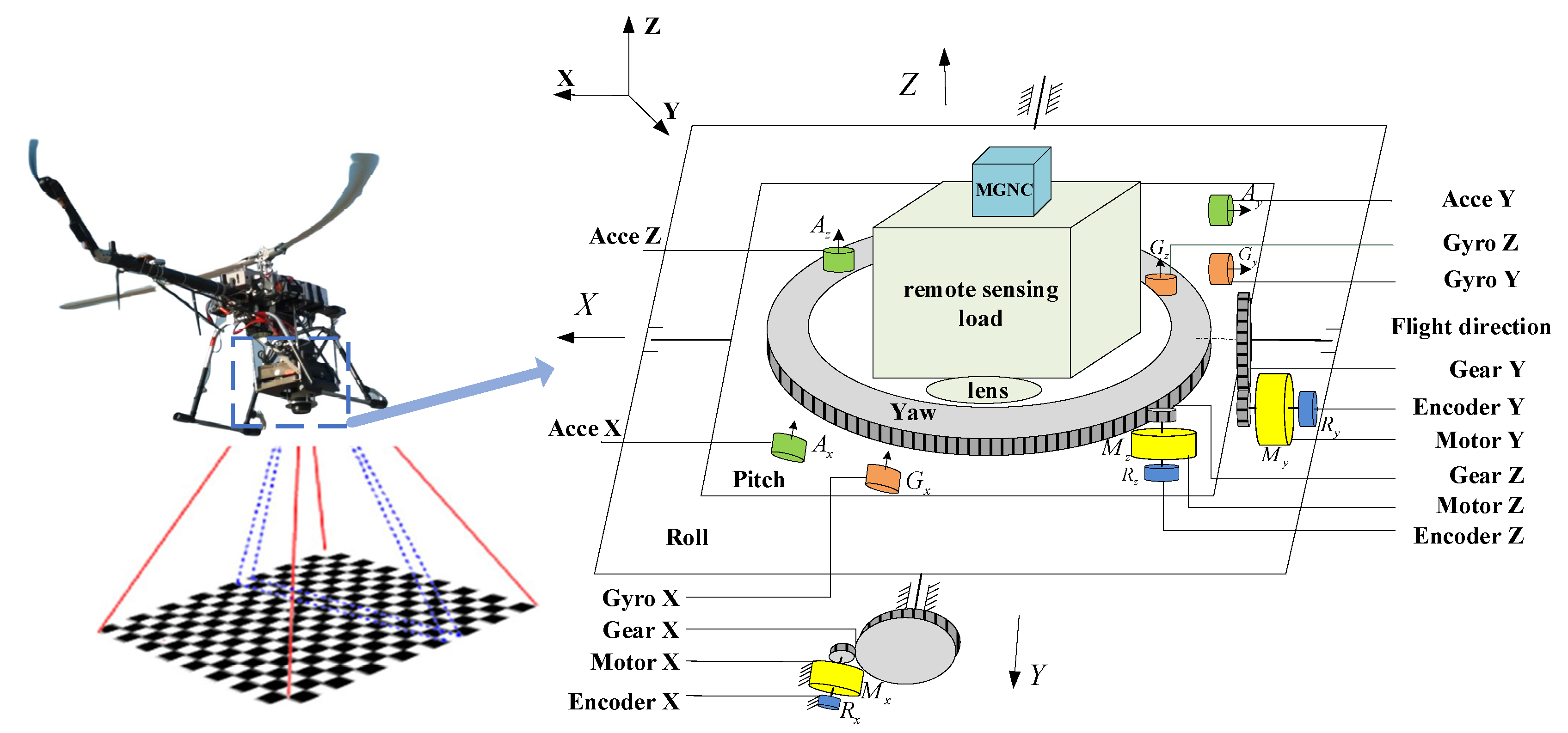
The schematic diagram of the three-axis ISP is shown in Figure 1, which is composed of the roll gimbal, pitch gimbal, and yaw gimbal. The roll gimbal is located at the outermost gimbal, fixed on the base by the shock absorbers. The pitch gimbal is adjacent to the roll gimbal, and the yaw gimbal is located in the innermost gimbal, carrying the remote sensing load. The frame structure of the ISP is symmetrically distributed from the inside to the outside, which ensures the stability of the LOS in the mechanical structure. The high-performance micro-guidance navigation control (MGNC) unit is installed on the top of the remote sensing load, which has the same base as the remote sensing load. Therefore, it can sample the pointing accuracy of the LOS of the remote sensing load in the geographic coordinate system and generate the corresponding control commands to isolate non-ideal disturbances. In order to achieve a high precision and a fast response control, the driving mechanisms of ISP are mainly composed of the brushless DC motors and wire gear drive systems. Based on the commands of the MGNC unit, the remote sensing load is adjusted correspondingly.

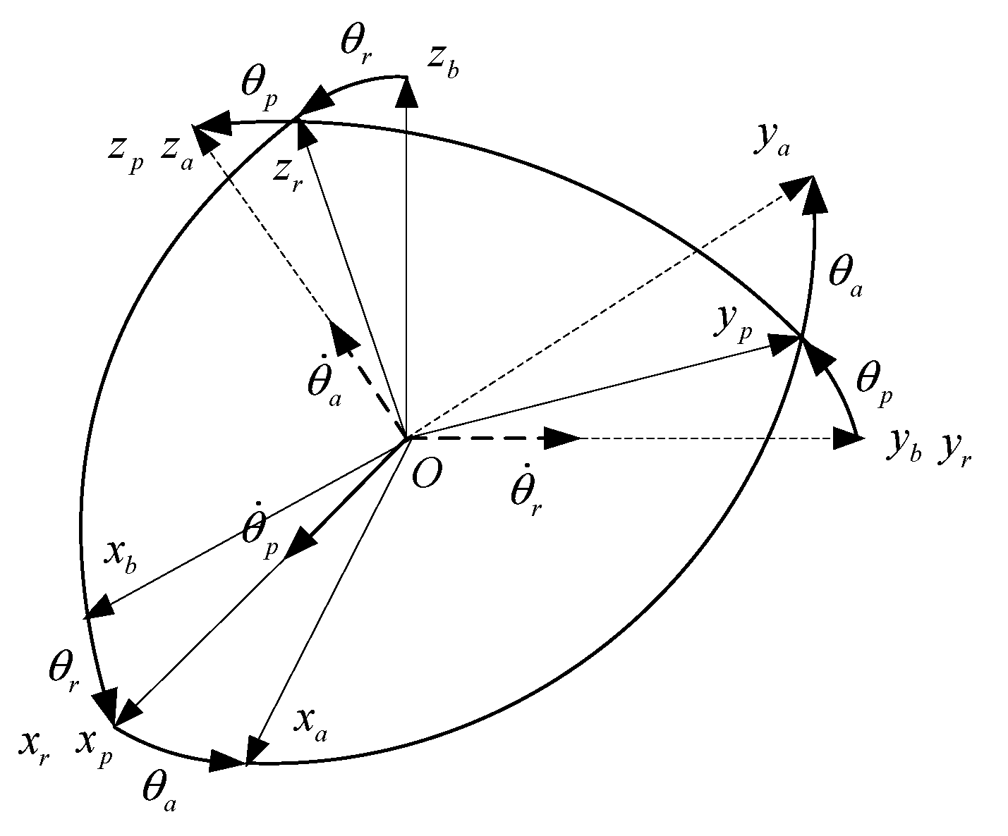
The coordinates used in the three-axis ISP system are shown in Figure 2. The $x_b$, $y_b$, $z_b$, $x_r$, $y_r$, $z_r$, $x_p$, $y_p$, $z_p$ and $x_a$, $y_a$, $z_a$ are the base coordinates, roll coordinates, pitch coordinates, and yaw coordinates, respectively. Moreover, the attitude and angular velocity of the ISP are defined as $\mathsf{\theta }={\left[\begin{array}{ccc}{\theta }_p& {\theta }_r& {\theta }_a\end{array}\right]}^T$ and $\dot{\mathsf{\theta }}={\left[\begin{array}{ccc}{\dot{\theta }}_p& {\dot{\theta }}_r& {\dot{\theta }}_a\end{array}\right]}^T$ with respect to the base coordinate obtained by the roll-pitch-yaw sequence of rotations. Define $B=p,r,a,b$ as the pitch coordinates, the roll coordinates, the yaw coordinates, and the base coordinates, respectively; ${\mathsf{\omega }}_{iB}^B={\left[\begin{array}{ccc}{\omega }_{iBx}^B& {\omega }_{iBy}^B& {\omega }_{iBz}^B\end{array}\right]}^T$ as the angular velocity of the $B$ coordinate with respect to the inertial coordinate expressed in the $B$ coordinate; ${\mathsf{\omega }}_{tB}^B={\left[\begin{array}{ccc}{\omega }_{tBx}^B& {\omega }_{tBy}^B& {\omega }_{tBz}^B\end{array}\right]}^T$ as the angular velocity of the $B$ coordinate with respect to the geographic coordinate expressed in the $B$ coordinate; ${\mathsf{\omega }}_{it}^t={\left[\begin{array}{ccc}{\omega }_{itx}^t& {\omega }_{ity}^t& {\omega }_{itz}^t\end{array}\right]}^T$ as the angular velocity of the geographic coordinate with respect to the inertial coordinate expressed in the geographic coordinate; $C_t^B$ as the transformation matrix from the geographic coordinates to the $B$ coordinates. Moreover, $C_b^r$, $C_r^p$, and $C_p^a$ represent the transformation matrixes from base coordinates to roll coordinates, roll coordinates to pitch coordinates, and pitch coordinates to yaw coordinates, respectively. According to Figure 2, $C_b^r$, $C_r^p$, and $C_p^a$ can be expressed as.

$$C_b^r=\left[\begin{array}{ccc}\cos {\theta }_r& 0& -\sin {\theta }_r\\ 0& 1& 0\\ \sin {\theta }_r& 0& \cos {\theta }_r\end{array}\right],C_r^p=\left[\begin{array}{ccc}1& 0& 0\\ 0& \cos {\theta }_p& \sin {\theta }_p\\ 0& -\sin {\theta }_p& \cos {\theta }_p\end{array}\right],C_p^a=\left[\begin{array}{ccc}\cos {\theta }_a& \sin {\theta }_a& 0\\ -\sin {\theta }_a& \cos {\theta }_a& 0\\ 0& 0& 1\end{array}\right]$$

Referring to the previous work [20], the dynamic model of the ISP can be defined as follows:

$$\begin{array}{l}{J}_{az}{\dot{\omega }}_{iaz}^a=N{K}_t\frac{u_a-K_{e}N({\omega }_{iaz}^a-{\omega }_{ibz}^a)}{R_m}\\ +(N{T}_{dm}+T_{da})+N(N-1)J_m{\dot{\omega }}_{ibz}^a-N^2{J}_m{\dot{\omega }}_{iaz}^a\end{array}$$

(1)

$$\begin{array}{l}{\left[\left(J_{px}+J_{ax}\right){\omega }_{ipx}^p\right]}^{\prime }=-\left(J_{px}+J_{ax}\right){\dot{\omega }}_{irx}^r+J_{az}{\omega }_{iaz}^a{\omega }_{ipy}^p\\ +\left(J_{pz}+J_{az}-J_{py}-J_{ay}\right){\omega }_{ipy}^p{\omega }_{ipz}^p+N{K}_t\frac{u_p-K_{e}N\left({\omega }_{ipx}^p-{\omega }_{ibx}^p\right)}{R_m}\\ +\left(N{T}_{dm}+T_{dp}\right)+N(N-1)J_m{\dot{\omega }}_{ibx}^p-N^2{J}_m{\dot{\omega }}_{ipx}^p\end{array}$$

(2)

$$\begin{array}{l}[J_{ry}{\omega }_{iry}^r+\cos {\theta }_p(J_{ay}+J_{py}){\omega }_{ipy}^p-\sin {\theta }_p(J_{az}+J_{pz}){\omega }_{ipz}^p-\sin {\theta }_p{J}_{az}{\omega }_{iaz}^a{]}^{\prime }\\ +(J_{rx}-J_{rz}){\omega }_{irx}^r{\omega }_{irz}^r+(J_{ax}+J_{px}){\omega }_{ipx}^p{\omega }_{irz}^r-\sin {\theta }_p(J_{ay}+J_{py}){\omega }_{ipy}^p{\omega }_{irx}^r\\ -\cos {\theta }_p(J_{az}+J_{pz}){\omega }_{ipz}^p{\omega }_{irx}^r-\cos {\theta }_p{J}_{az}{\omega }_{iaz}^a{\omega }_{irx}^r=N{K}_t\frac{u_r-K_{e}N({\omega }_{iry}^r-{\omega }_{iby}^r)}{R_m}\\ +(N{T}_{dm}+T_{dr})+N(N-1)J_m{\dot{\omega }}_{iby}^r-N^2{J}_m{\dot{\omega }}_{iry}^r\end{array}$$

(3)

where ${\omega }_{ibz}^a$, ${\dot{\omega }}_{ibz}^a$, ${\omega }_{ibx}^p$, ${\dot{\omega }}_{ibx}^p$, ${\omega }_{iby}^r$, and ${\dot{\omega }}_{iby}^r$ can be obtained by ${\mathsf{\omega }}_{ib}^b$, ${\dot{\omega }}_{ib}^b$ and the transformation matrices $C_b^r$, $C_r^p$, and $C_p^a$. $J_p=diag(J_{px},J_{py},J_{pz})$, $J_r=diag(J_{rx},J_{ry},J_{rz})$ and $J_a=diag(J_{ax},J_{ay},J_{az})$ are the moment of inertia of pitch, roll, and yaw gimbal in three directions, respectively, and they are all symmetric matrices. $J_m$ is the moment of inertia of the motor. $K_t$ is the torque sensitivity. $K_e$ is the back EMF constant. $R_m$ is the motor resistance. The $N$ is the gear ratio of motor. $u_p$, $u_r$, and $u_a$ are the voltage inputs applied on the pitch, roll, and yaw gimbal motor armatures, respectively. $T_{dp}$, $T_{dr}$, and $T_{da}$ are the torque disturbances imposed on the pitch gimbal, roll gimbal, and yaw gimbal, respectively. $T_{dm}$ is the torque disturbance imposed on the motor of ISP.

The attitudes of the LOS are the criteria of the ISP system, which are defined in the geographic coordinates. However, it is obvious that the $\mathsf{\theta }$ and $\dot{\mathsf{\theta }}$ of the ISP of [20] are measured in the inertial coordinates. The process of converting from inertial coordinates to geographic coordinates is complicated, which will increase the computational burden of the MGNC unit and reduce the measurement and control performance. In order to solve the above problem, a nonlinear dynamic model based on the geographic coordinates is proposed. The $\mathsf{\theta }$ and $\dot{\mathsf{\theta }}$ of the ISP with respect to geographic coordinates is expressed as $\mathsf{\theta }={\left[\begin{array}{ccc}{\theta }_{tp}^p& {\theta }_{tr}^r& {\theta }_{ta}^a\end{array}\right]}^T$ and $\dot{\mathsf{\theta }}={\left[\begin{array}{ccc}{\omega }_{tpx}^p& {\omega }_{try}^r& {\omega }_{taz}^a\end{array}\right]}^T$, and the corresponding values can be measured by the MGNC unit. The parameters coordinates can be unified:

$${\mathsf{\omega }}_{iB}^B=C_t^B{\mathsf{\omega }}_{it}^t+{\mathsf{\omega }}_{tB}^B,B=p,r,a,b$$

(4)

Since ${\mathsf{\omega }}_{it}^t$ is relatively small.

$${\mathsf{\omega }}_{iB}^B\approx {\mathsf{\omega }}_{tB}^B,B=p,r,a,b$$

(5)

To facilitate the application in practical engineering, based on (1)–(5), the nonlinear dynamic model of the three-axis ISP based on the geographic coordinates can be obtained as follows, and the detailed information on the dynamic model is shown in the Appendix A.

$${\dot{\omega }}_{tax}^a=f_1(t)+b_1{u}_1+g_1{d}_1=b_1{u}_1+D_1$$

(6)

$${\dot{\omega }}_{tay}^a=f_2(t)+b_2{u}_2+g_2{d}_2=b_2{u}_2+D_2$$

(7)

$${\dot{\omega }}_{taz}^a=f_3(t)+b_3{u}_3+g_3{d}_3=b_3{u}_3+D_3$$

(8)

where:

$$\begin{array}{ll}{f}_1(t)=& -(\frac{K_t{K}_e{N}^2}{J_2{R}_m}+(s_1-{\dot{\theta }}_a)\tan {\theta }_a){\omega }_{tax}^a+(\frac{K_t{K}_e{N}^2}{J_2{R}_m}\tan {\theta }_a-s_1\cos {\theta }_p){\omega }_{tay}^a\\ & +\frac{s_1{J}_2\sin {\theta }_p+J_{az}{\omega }_{tpy}^p}{J_2\cos {\theta }_a}{\omega }_{taz}^a+\frac{K_t{K}_e{N}^2{\omega }_{trx}^p+N(N-1)R_m{J}_m{\dot{\omega }}_{trx}^p}{J_2{R}_m\cos {\theta }_a}-\frac{s_1}{\cos {\theta }_a}\\ & -\frac{(J_{pz}-J_{py}-J_{ay}){\omega }_{trz}^r{}^2\sin {\theta }_p\cos {\theta }_p+J_2({\omega }_{tay}^a\sin {\theta }_a{)}^{\prime }}{J_2\cos {\theta }_a}{\dot{\theta }}_a\sin {\theta }_p\end{array}$$

$$\begin{array}{ll}{f}_2(t)=& -(\frac{K_t{K}_e{N}^2}{J_3{R}_m}\tan {\theta }_a+s_2\tan {\theta }_a+\frac{(J_{ax}+J_{px}){\omega }_{trz}^r}{J_3\cos {\theta }_p}){\omega }_{tax}^a-(\frac{K_t{K}_e{N}^2}{J_3{R}_m}+s_2\\ & -\frac{(J_{ax}+J_{px}){\omega }_{trz}^r}{J_3\cos {\theta }_p}\tan {\theta }_a){\omega }_{tay}^a+\frac{(K_t{K}_e{N}^2+J_3{R}_m{s}_2)\tan {\theta }_p+J_{az}{R}_m{\omega }_{trx}^r}{J_3{R}_m\cos {\theta }_a}{\omega }_{iaz}^a\\ & +\frac{K_t{K}_e{N}^2{\omega }_{tby}^r+N(N-1)J_m{R}_m{\dot{\omega }}_{tby}^r}{J_3{R}_m\cos {\theta }_a\cos {\theta }_p}-(\frac{K_t{K}_e{N}^2}{J_3{R}_m}+s_2)\frac{\tan {\theta }_p}{\cos {\theta }_a}{\dot{\theta }}_a\\ & +\frac{(J_{ay}+J_{py}){\sin }^2{\theta }_p+J_{pz}{\cos }^2{\theta }_p-J_{rx}+J_{rz}}{J_3\cos {\theta }_a\cos {\theta }_p}{\omega }_{trz}^r{\omega }_{trx}^r\\ & -\frac{[(J_{ay}+J_{py}-J_{az}-J_{pz}){\omega }_{trz}^r\cos {\theta }_p\sin {\theta }_p-\sin {\theta }_p{J}_{az}{\dot{\theta }}_a{]}^{\prime }}{J_3\cos {\theta }_a\cos {\theta }_p}\\ & -\frac{({\omega }_{tax}^a\sin {\theta }_a\cos {\theta }_p-{\omega }_{taz}^a\sin {\theta }_p+{\dot{\theta }}_a\sin {\theta }_p{)}^{\prime }+{\omega }_{tay}^a(\cos {\theta }_a\cos {\theta }_p{)}^{\prime }}{\cos {\theta }_a\cos {\theta }_p}\end{array}$$

$f_3(t)=\frac{K_t{K}_e{N}^2({\omega }_{tbz}^a-{\omega }_{taz}^a)}{J_1{R}_m}+\frac{N(N-1)J_m{\dot{\omega }}_{tbz}^a}{J_1}$, $b_1=\frac{N{K}_t}{J_2{R}_m\cos {\theta }_a}$, $b_2=\frac{N{K}_t}{J_3{R}_m\cos {\theta }_a\cos {\theta }_p}$, $b_3=\frac{N{K}_t}{J_1{R}_m}$, $u_1=u_p$, $u_2=u_r$, $u_3=u_a$, $g_1=\frac{1}{J_2\cos {\theta }_a}$, $g_2=\frac{1}{J_3\cos {\theta }_a\cos {\theta }_p}$, $g_3=\frac{1}{J_1}$, $d_1=N{T}_{dm}+T_{dp}+{\mathsf{\Delta }}_1$, $d_2=N{T}_{dm}+T_{dr}+{\mathsf{\Delta }}_2$, $d_3=N{T}_{dm}+T_{da}+{\mathsf{\Delta }}_3$, ${\mathsf{\Delta }}_i$ denotes the unknown uncertainties of $f_i(t)$ and $d_i$, $i=1,2,3$, $D_i=f_i(t)+g_i{d}_i$, $i=1,2,3$ denotes the lumped disturbance, which contains nonlinearities and various unmodeled disturbances of the ISP system.

3. Control System of the ISP

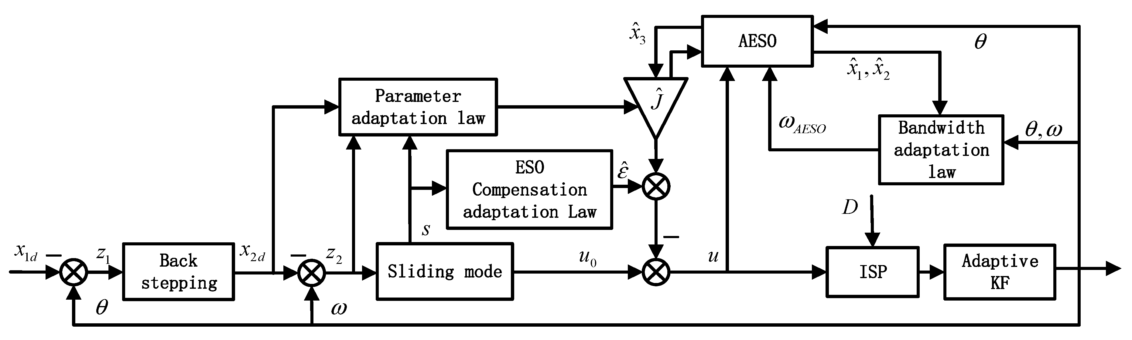
Since $D_i$, $i=1,2,3$ are nonlinear and time variant functions, it is difficult to express them accurately in the actual control system, which will affect the control performance of the ISP. Therefore, a compound control method based on the AESO and the adaptive back-stepping integral SMC is proposed. The adaptive back-stepping integral SMC method is proposed to handle the ISP system nonlinearity, parameter variations, and disturbances. Furthermore, the sign function is replaced by the lumped disturbance estimation of AESO, which can reduce the chattering problem and improve the control performance.

Since the pitch, roll, and yaw gimbals have the same control structure, take the roll gimbal as an example, and let $\theta ={\theta }_r$, $\omega ={\omega }_{tay}^a$, $J=1/b=1/b_2$, $u=u_2$, $D=D_2$, the control flowchart is shown in Figure 3.

3.1. The Traditional Linear ESO

For the ISP, let ${\left[\begin{array}{ccc}{x}_1& x_2& x_3\end{array}\right]}^T={\left[\begin{array}{ccc}\theta & \omega & D\end{array}\right]}^T$, where $x_i(t),i=1,2,3$ are the state variables.

Assumption 1.

The $D(t)$ and its first derivative $\dot{D}(t)=h(t)$are bounded, satisfying $\left|D(t)\right|\le H$,$\left|h(t)\right|\le {\delta }_{h(t)}$.

From (7), the expansion state equation of ISP can be obtained as:

$$\left\{\begin{array}{l}{\dot{x}}_1=x_2\hfill \\ {\dot{x}}_2=bu+x_3\hfill \\ {\dot{x}}_3=h\hfill \end{array}\right.$$

(9)

For the (9), design the linear ESO (LESO).

$$\left\{\begin{array}{l}{e}_1={\widehat{x}}_1-x_1\hfill \\ {\dot{\widehat{x}}}_1={\widehat{x}}_2-3{\omega }_o{e}_1\hfill \\ {\dot{\widehat{x}}}_2={\widehat{x}}_3+b_{0}u-3{\omega }_o^2{e}_1\hfill \\ {\dot{\widehat{x}}}_3=-{\omega }_o^3{e}_1\hfill \end{array}\right.$$

(10)

where ${\widehat{x}}_1$, ${\widehat{x}}_2$ and ${\widehat{x}}_3$ are the estimation value of $x_1$, $x_2$ and $x_3$, $e_1$ is the error between ${\widehat{x}}_1$ and $x_1$, ${\omega }_o$ is the fixed bandwidth of LESO. At the same time, $b_0$ is the estimation value of $b$.

Based on the (10), we can obtain:

$${\widehat{x}}_1=\frac{(3{\omega }_o{s}^2+3{\omega }_o^{2}s+{\omega }_o^3)x_1+bsu}{s^3+3{\omega }_o{s}^2+3{\omega }_o^{2}s+{\omega }_o^3}$$

(11)

$${\widehat{x}}_3=\frac{{\omega }_o^3(s^2{x}_1-bu)}{s^3+3{\omega }_o{s}^2+3{\omega }_o^{2}s+{\omega }_o^3}$$

(12)

According to (9), one has:

$$D=x_3={\dot{x}}_2-bu={\ddot{x}}_1-bu$$

(13)

Combining (13) and (12), the lumped disturbance observation transfer function can be defined as follows:

$$G_D(s)=\frac{{\widehat{x}}_3}{D}=\frac{{\omega }_o^3}{s^3+3{\omega }_o{s}^2+3{\omega }_o^{2}s+{\omega }_o^3}={\left(\frac{{\omega }_o}{s+{\omega }_o}\right)}^3$$

(14)

The frequency response of $G_D(s)$ is shown in Figure 4. It can be seen that as the frequency of the disturbance increases, the estimation of the disturbance by LESO exhibits obvious phase lag and amplitude attenuation. The decrease in the disturbance estimation accuracy will result in a decrease in the control performance. Although increasing the observation bandwidth ${\omega }_o$ can improve the estimation ability of LESO, it will also introduce more high-frequency noise, which will weaken the system’s resistance to high-frequency noise.

Moreover, define:

$$\tilde{x}=\left[\begin{array}{ccc}{\tilde{x}}_1& {\tilde{x}}_2& {\tilde{x}}_3\end{array}\right], {\tilde{x}}_i(t)=x_i(t)-{\widehat{x}}_i(t), i=1,2,3$$

(15)

By subtracting (10) from (9), the error model of the LESO is:

$$\begin{array}{l}{\dot{\tilde{x}}}_1(t)={\tilde{x}}_2(t)-3{\omega }_o{\tilde{x}}_1(t)\\ {\dot{\tilde{x}}}_2(t)={\tilde{x}}_3(t)-3{\omega }_o^2{\tilde{x}}_1(t)\\ {\dot{\tilde{x}}}_3(t)=h(t)-{\omega }_o^3{\tilde{x}}_1(t)\end{array}$$

(16)

According to (16), one has:

$${\tilde{x}}_3(t)={\dot{\tilde{x}}}_2(t)+3{\omega }_o^2(t){\tilde{x}}_1(t)$$

(17)

when there are certain errors between the real states $x_1$ and $x_2$ of the system and the observation states ${\widehat{x}}_1$ and ${\widehat{x}}_2$ of LESO, the disturbance estimation error makes the corresponding increment due to the high observation bandwidth. Therefore, it will cause a great peaking phenomenon.

3.2. The AESO

To overcome the problem of LESO, we propose an AESO.

$$\left\{\begin{array}{l}{e}_1={\widehat{x}}_1-x_1\hfill \\ {\dot{\widehat{x}}}_1={\widehat{x}}_2-3{\omega }_{AESO}(\tilde{x})e_1\hfill \\ {\dot{\widehat{x}}}_2={\widehat{x}}_3+\widehat{b}u-3{\omega }_{AESO}^2(\tilde{x})e_1\hfill \\ {\dot{\widehat{x}}}_3=-{\omega }_{AESO}^3(\tilde{x})e_1\hfill \end{array}\right.$$

(18)

where $\widehat{b}$ is the input gain value estimated by the $\dot{\widehat{J}}$, and $\dot{\widehat{J}}$ is the parameter adaptation law to be synthesized later. ${\omega }_{AESO}(\tilde{x})={\omega }_0\exp (-{\tilde{x}}_o^T\mathsf{\delta }{\tilde{x}}_o)$ with ${\tilde{x}}_o={\left[\begin{array}{cc}{\tilde{x}}_1& {\tilde{x}}_2\end{array}\right]}^T$, $\mathsf{\delta }=\left[\begin{array}{ll}1/\delta \hfill & 0\hfill \\ 0\hfill & 1/({\omega }_0^2\delta )\hfill \end{array}\right]$, is the bandwidth of AESO, which is composed by the observation errors of $x_1$ and $x_2$, and the constant $\delta >0$ needs to be designed.

Remark 

1. The input gain$\widehat{b}$and observation bandwidth${\omega }_{AESO}(\tilde{x})$of AESO are adaptive values, which are different from LESO. Adaptive variation of $\widehat{b}$can reduce the estimation burden of AESO [28]. In addition, through the data input of the observation errors ${\tilde{x}}_o={\left[\begin{array}{cc}{\tilde{x}}_1& {\tilde{x}}_2\end{array}\right]}^T$, the observation bandwidth ${\omega }_{AESO}(\tilde{x})$ can deal with the peaking phenomenon, improving the estimation accuracy of AESO without introducing excessive high-frequency noise. In order to further ensure the reliability of AESO, define:

$${\omega }_{AESO}(\tilde{x})=\left\{\begin{array}{ll}{\omega }_0\exp (-{\tilde{x}}_o^T\delta {\tilde{x}}_o)\hfill & {\omega }_{AESO}(\tilde{x})\ge {\omega }_{\min }\\ {\omega }_{\min }\hfill & {\omega }_{AESO}(\tilde{x})<{\omega }_{\min } \end{array}\right.$$

Convergence Proof.

Let ${\zeta }_i(t)=({\tilde{x}}_i(t))/({\omega }_0^{i-1}),i=1,2,3$, from (16) and (18), one has

$$\dot{\zeta }={\omega }_0{A}_{\zeta }(\zeta )\zeta +B_{\zeta }\frac{h(t)}{{\omega }_0^2}$$

(19)

where $\zeta ={[\begin{array}{ccc}{\zeta }_1& {\zeta }_2& {\zeta }_3\end{array}]}^T\in {ℝ}^3$, $A_{\zeta }(\zeta )=\left[\begin{array}{ccc}-3\exp (-({\zeta }_1^2+{\zeta }_2^2)/\delta )& 1& 0\\ -3\exp (-({\zeta }_1^2+{\zeta }_2^2)/\delta )& 0& 1\\ -\exp (-({\zeta }_1^2+{\zeta }_2^2)/\delta )& 0& 0\end{array}\right]$ and $B_{\zeta }={\left[\begin{array}{ccc}0& 0& 1\end{array}\right]}^T$. □

Theorem 1.

For (18), if$\delta >m^2/0.9$($m>0$) and$V_{\zeta }(\zeta (0))\le m^2/(3{\omega }_0)$, there exist a constant ${\sigma }_i>0$and a finite time $T_1>0$, satisfying

$$\left|{\tilde{x}}_i(t)\right|\le {\sigma }_i, {\sigma }_i=\frac{8{\delta }_{h(t)}}{{\omega }_0^{4-i}}, i=1,2,3, \forall t\ge T_1$$

(20)

Proof. 

The autonomous system of (19) is:

$$\dot{\zeta }={\omega }_0{A}_{\zeta }(\zeta )\zeta$$

(21)

For (21), define the Lyapunov function $V_{\zeta }(\mathsf{\zeta })=(1/{\omega }_0){\mathsf{\zeta }}^T{P}_0\mathsf{\zeta }$ with $A_0^T{P}_0+P_0{A}_0=-I_3$, where $A_0=\left[\begin{array}{ccc}-3& 1& 0\\ -3& 0& 1\\ -1& 0& 0\end{array}\right]$ and $P_0=\left[\begin{array}{ccc}1& -0.5& -1\\ -0.5& 1& -0.5\\ -1& -0.5& 4\end{array}\right]$. Then, the ${\dot{V}}_{\zeta }(\mathsf{\zeta })$ is.

$${\dot{V}}_{\zeta }(\mathsf{\zeta })={\zeta }^T(A_{\zeta }{(\zeta )}^T{P}_0+P_0{A}_{\zeta }(\mathsf{\zeta }))\mathsf{\zeta }$$

(22)

If $\delta >m^2/0.9$ and $V_{\zeta }(\mathsf{\zeta }(0))\le m^2/(3{\omega }_0)$ are achievable, then ${‖{\zeta }_o‖}_2\le m, {\zeta }_o=\left[\begin{array}{cc}{\zeta }_1& {\zeta }_2\end{array}\right]$, $A_{\zeta }{(\zeta )}^T{P}_0+P_0{A}_{\zeta }(\mathsf{\zeta })<0$, and $\mathsf{\zeta }=0$ of (21) are locally exponentially stable (Theorem 1 of [29]).

Based on the Assumption 1 and the exponential stability of (21), for (19), there exists an invariant set:

$$B_0\triangleq \left\{\zeta \in {ℝ}^3: {‖\zeta ‖}_2\le \frac{2{\lambda }_{\max }\left(P_0{B}_{\zeta }\right){\delta }_{h(t)}}{{\omega }_0^3}=\frac{8{\delta }_{h(t)}}{{\omega }_0^3}\right\}$$

(23)

for any $\mathsf{\zeta }\notin B_0$ and $V_{\zeta }(\mathsf{\zeta })\le m^2/(3{\omega }_0)$, we can obtain.

$${\dot{V}}_{\zeta }(\mathsf{\zeta })={\zeta }^T\left(A_{\zeta }{(\zeta )}^T{P}_0+P_0{A}_{\zeta }(\zeta )\right)\mathsf{\zeta }+2{\zeta }^T{P}_0{B}_{\zeta }\frac{{\delta }_{h(t)}}{{\omega }_0^3}<0$$

(24)

then, for all $t\ge T_1$, considering ${\zeta }_i(t)=({\tilde{x}}_i(t))/({\omega }_0^{i-1}),i=1,2,3$ and (24), one has

$$\left|{\tilde{x}}_i(t)\right|\le {\omega }_0^{i-1}{‖\zeta ‖}_2\le \frac{8{\delta }_{h(t)}}{{\omega }_0^{4-i}}={\sigma }_i$$

(25)

□

3.3. The Compound Control Method Based on the AESO and the Adaptive Back-Stepping Integral SMC

To facilitate the design of adaptation laws, for (9), we can obtain:

$$\left\{\begin{array}{l}{\dot{x}}_1=x_2\hfill \\ J{\dot{x}}_2=u+D_J\hfill \end{array}\right.$$

(26)

where $J=1/b$, $D_J=D/b$.

Assumption 2.

Define the unknown parameter $J\in {\mathsf{\Omega }}_J\triangleq \left\{J\in ℝ:J_{\min }\le J\le J_{\max }\right\}$, and the $\widehat{J}=1/\widehat{b}$is the estimation value of $J$. Moreover, define the lumped disturbance estimation error $\epsilon =D_J-\widehat{J}{\widehat{x}}_3$,$\epsilon \in {\mathsf{\Omega }}_{\epsilon }\triangleq \left\{\epsilon \in ℝ:{\epsilon }_{\min }\le \epsilon \le {\epsilon }_{\max }\right\}$and the lumped disturbance estimation compensation $\widehat{\epsilon }$is the estimation value of $\epsilon$.

Let the estimation error $\tilde{J}=\widehat{J}-J$, $\tilde{\epsilon }=\widehat{\epsilon }-\epsilon$. Combining Assumption 2, the adaptation law $\dot{\widehat{J}}$ and $\dot{\widehat{\epsilon }}$, with $J_{\min }\le \widehat{J}(0)\le J_{\max }$ and ${\epsilon }_{\min }\le \widehat{\epsilon }(0)\le {\epsilon }_{\max }$, can be defined as [28].

$$\dot{\widehat{J}}=Pro{j}_{\widehat{J}}({\tau }_{\widehat{J}})=\left\{\begin{array}{l}0, if \widehat{J}\ge J_{\max } and {\tau }_{\widehat{J}}>0\hfill \\ 0, if \widehat{J}\le J_{\min } and {\tau }_{\widehat{J}}<0\hfill \\ {\tau }_{\widehat{J}} otherwise\hfill \end{array}\right.$$

(27)

$$\dot{\widehat{\epsilon }}=Pro{j}_{\widehat{\epsilon }}({\tau }_{\widehat{\epsilon }})=\left\{\begin{array}{l}0, if \widehat{\epsilon }\ge {\epsilon }_{\max } and {\tau }_{\widehat{\epsilon }}>0\hfill \\ 0, if \widehat{\epsilon }\le {\epsilon }_{\min } and {\tau }_{\widehat{\epsilon }}<0\hfill \\ {\tau }_{\widehat{\epsilon }} otherwise\hfill \end{array}\right.$$

(28)

where ${\tau }_{\widehat{J}}$ and ${\tau }_{\widehat{\epsilon }}$ are the adaptation functions to be synthesized later; for any adaption function, the projection mapping used in (27) and (28) guarantees $\widehat{J}\in {\mathsf{\Omega }}_{\widehat{J}}\triangleq \left\{\widehat{J}\in ℝ:J_{\min }\le \widehat{J}\le J_{\max }\right\}$, $\widehat{\epsilon }\in {\mathsf{\Omega }}_{\widehat{\epsilon }}\triangleq \left\{\widehat{\epsilon }\in ℝ:{\epsilon }_{\min }\le \widehat{\epsilon }\le {\epsilon }_{\max }\right\}$.

Define the desired attitude angle $x_{1d}$, the virtual control law $x_{2d}$ and the state error as:

$$z_1=x_1-x_{1d} z_2=x_2-x_{2d}$$

(29)

and the derivative of $z_1$ is obtained by:

$${\dot{z}}_1=x_2-{\dot{x}}_{1d}$$

(30)

For the virtual control law $x_{2d}$, define:

$$x_{2d}=-k_1{z}_1+{\dot{x}}_{1d}$$

(31)

where the constant $k_1>0\in ℝ$ is the virtual control law coefficient.

Define the first Lyapunov function $V_1=\frac{1}{2}{z}_1^2$, then the ${\dot{V}}_1$ is.

$${\dot{V}}_1=z_1{\dot{z}}_1=z_1\left(x_2-{\dot{x}}_{1d}\right)=z_1\left(x_2-x_{2d}-k_1{z}_1\right)=z_1{z}_2-k_1{z}_1^2$$

(32)

It is obvious that if $z_2$ converges to zero, $z_1$ is asymptotically stable, and $x_1$ can asymptotically track $x_{1d}$.

Based on (26) and (29), the differentiation of $z_2$ is.

$$J{\dot{z}}_2=u+D_J-J{\dot{x}}_{2d}$$

(33)

Define the integral sliding surface $s$ as.

$$s=z_2+k_2{\displaystyle \int z_{2}d\tau }$$

(34)

where $k_2\in ℝ$ is a positive constant. Then, the control law $u$, the adaptation functions ${\tau }_{\widehat{J}}$ and ${\tau }_{\widehat{\epsilon }}$ can be designed as.

$$u=u_0-(\widehat{J}{\widehat{x}}_3+\widehat{\epsilon })=\widehat{J}({\dot{x}}_{2d}-k_2{z}_2)-k_{s}s-(\widehat{J}{\widehat{x}}_3+\widehat{\epsilon })$$

(35)

$${\tau }_{\widehat{J}}=-{\gamma }_{J}s({\dot{x}}_{2d}-k_2{z}_2)$$

(36)

$${\tau }_{\widehat{\epsilon }}={\gamma }_{\epsilon }s$$

(37)

where $k_s\in ℝ$ is a positive constant, ${\gamma }_J\in ℝ$ and ${\gamma }_{\epsilon }\in ℝ$ are the learning rates.

Stability analysis:

Define the second Lyapunov function $V_2=\frac{1}{2}J{s}^2+\frac{1}{2{\gamma }_J}{\tilde{J}}^2+\frac{1}{2{\gamma }_{\epsilon }}{\tilde{\epsilon }}^2$, then the ${\dot{V}}_2$ is.

$$\begin{array}{ll}{\dot{V}}_2& =Js\dot{s}+\frac{1}{{\gamma }_J}\tilde{J}\dot{\widehat{J}}+\frac{1}{{\gamma }_{\epsilon }}\tilde{\epsilon }\dot{\widehat{\epsilon }}=s(J{\dot{z}}_2+J{k}_2{z}_2)+\frac{1}{{\gamma }_J}\tilde{J}\dot{\widehat{J}}+\frac{1}{{\gamma }_{\epsilon }}\tilde{\epsilon }\dot{\widehat{\epsilon }}\\ & =s(u+D_J-J({\dot{x}}_{2d}-k_2{z}_2))+\frac{1}{{\gamma }_J}\tilde{J}\dot{\widehat{J}}+\frac{1}{{\gamma }_{\epsilon }}\tilde{\epsilon }\dot{\widehat{\epsilon }}\end{array}$$

(38)

Taking (35)–(37) into (38).

$$\begin{array}{ll}{\dot{V}}_2& =s(\widehat{J}({\dot{x}}_{2d}-k_2{z}_2)-k_{s}s-(\widehat{J}{\widehat{x}}_3+\widehat{\epsilon })+D_J-J({\dot{x}}_{2d}-k_2{z}_2))+\frac{1}{{\gamma }_J}\tilde{J}\dot{\widehat{J}}+\frac{1}{{\gamma }_{\epsilon }}\tilde{\epsilon }\dot{\widehat{\epsilon }}\\ & =s(\tilde{J}({\dot{x}}_{2d}-k_2{z}_2)-k_{s}s-(\widehat{J}{\widehat{x}}_3+\widehat{\epsilon })+D_J)+\frac{1}{{\gamma }_J}\tilde{J}\dot{\widehat{J}}+\frac{1}{{\gamma }_{\epsilon }}\tilde{\epsilon }\dot{\widehat{\epsilon }}\\ & =s(\tilde{J}({\dot{x}}_{2d}-k_2{z}_2)-k_{s}s-\tilde{\epsilon })+\frac{1}{{\gamma }_J}\tilde{J}\dot{\widehat{J}}+\frac{1}{{\gamma }_{\epsilon }}\tilde{\epsilon }\dot{\widehat{\epsilon }}\\ & =-k_s{s}^2+\tilde{J}(s({\dot{x}}_{2d}-k_2{z}_2)+\frac{1}{{\gamma }_J}\dot{\widehat{J}})+\tilde{\epsilon }(-s+\frac{1}{{\gamma }_{\epsilon }}\dot{\widehat{\epsilon }})\\ & =-k_s{s}^2\le 0\end{array}$$

(39)

Then, based on the $x_{2d}$ and $u$, the sliding surface $s=0$ is reachable. Meanwhile, the $x_1$ can track the $x_{1d}$ effectively.

Remark 2.

It is obvious that the control law $u$does not contain symbolic function $\mathrm{sgn}(s)$, which can reduce the chattering problem for the switching action of $\mathrm{sgn}(s)$and decrease the loss of actuators in the control system. Moreover, the estimation compensation $\widehat{\epsilon }$in $u$can improve the estimation accuracy of AESO.

Remark 3.

The projection mapping adaptation law (27) and (28) can guarantee $\tilde{J}(s({\dot{x}}_{2d}-k_2{z}_2)+\frac{1}{{\gamma }_J}\dot{\widehat{J}})\le 0$and $\tilde{\epsilon }(-s+\frac{1}{{\gamma }_{\epsilon }}\dot{\widehat{\epsilon }})\le 0$, thus guaranteeing ${\dot{V}}_2\le 0$. Since $V_2\ge 0$,${\dot{V}}_2\le 0$, when $t\to \infty$,$V_2$is bounded, and it can be shown that $\widehat{J}$is bounded. However, due to ${\dot{V}}_2=-k_s{s}^2$, when $s=0$,${\dot{V}}_2=0$, and $V_2$is not decreasing, which does not guarantee $\tilde{J}\to 0$. However, $\dot{\widehat{J}}$can still reduce the error between the estimation value $\widehat{b}$and the real input gain $b$.

4. Simulations, Experiments and Discussion

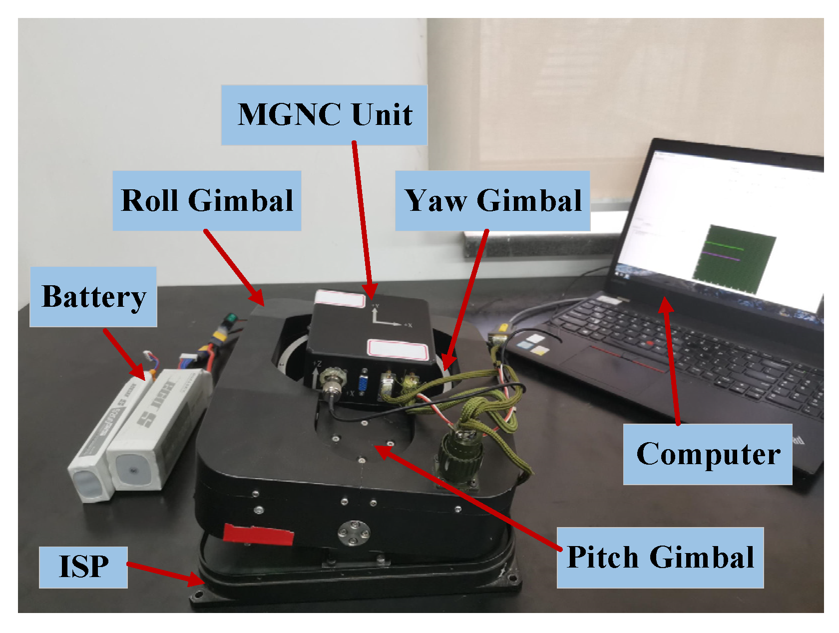
The three-axis ISP is shown in Figure 5. Its length, width, and height are 0.33 m, 0.255 m, and 0.115 m, respectively. With the camera, the total weight reaches 13 Kg. Based on the MGNC unit, ISP can get attitude errors and make corresponding control commands.

4.1. Simulations

Table 1. Parameters of the ISP.

Parameter	Value	Unit
$K_t$	$0.175$	Nm/Amp
$K_e$	$0.143$	V/rad/s
$R_m$	$4.15$	Ohms
$J_m$	$1.4\times {10}^{-4}$	Kg m2
$N$	$106.2$	Kg m2
$J_p$	$diag(0.20,0.267,0.46)$	Kg m2
$J_r$	$diag(0.30,0.25,0.71)$	Kg m2
$J_a$	$diag(0.54,0.453,0.184)$	Kg m2

shows the parameters of ISP. The battery voltage of the ISP system is 24 V, and the relationship between the input voltage $u_{voltage}$ of the ISP and the output value $u_{controller}$ of the controller is $u_{voltage}=\frac{24V}{1000}{u}_{controller}$.

With the analysis of disturbances in the ISP system [30], the corresponding asymmetrical disturbances have been added in simulations.

For the ISP system, the maximum mass imbalance distance is 5 mm, the maximum weight of the loads is 30 kg, and the amplitude of the wind disturbance is 1.5. Therefore, the torque disturbance $T_{dL}(L=p,r,a)$ can be obtained as:

$$T_{dL}=(2\times 30\times 9.8\times 0.005+1.5)\times (rand(t)-0.5)$$

(40)

The sliding friction coefficient of the ISP system is $\mu =0.1$. The weight and the radius of the motor gear in the ISP system are 0.5 Kg and 0.1 m, respectively, and the amplitude of the residual periodic vibration disturbances is 0.9. Therefore, the torque disturbance $T_{dm}$ can be defined as:

$$T_{dm}=(0.1\times 0.5\times 9.8\times 0.1+09)\times (\sin ({\omega }_{dm}t)+\sin (2{\omega }_{dm}t))$$

(41)

where ${\omega }_{dm}$ is the residual vibration frequency.

Moreover, the mean and standard deviation of the measurement noise are 0 and 0.01, so one has:

$$d_{noise}=normrnd(0,0.01)$$

(42)

In the simulation section, take the roll gimbal as an example, and the simulation time as 10 s. Let $x_{1d}=5°$, the initial ISP system state values $x_1(0)$ and $x_2(0)$ are $-5°$ and $-0.15°/\mathrm{s}$ respectively, and the initial AESO state values ${\left[\begin{array}{ccc}{\widehat{x}}_1(0)& {\widehat{x}}_2(0)& {\widehat{x}}_3(0)\end{array}\right]}^T={\left[\begin{array}{ccc}0& 0& 0\end{array}\right]}^T$.

In order to verify the control performance of the proposed method, the following three control algorithms are selected in the simulation part:

(1) The proposed method: the control law in (35) with $k_1=20$, $k_2=50$, $k_s=0.1$, ${\omega }_0=50$, $\delta =0.01$, ${\omega }_{\min }=10$, $\widehat{b}(0)=1.3$, $\widehat{\epsilon }(0)=0$, $\left[\begin{array}{cc}{J}_{\min }& J_{\max }\end{array}\right]=\left[\begin{array}{cc}0.5& 1\end{array}\right]$, $\left[\begin{array}{cc}{\epsilon }_{\min }& {\epsilon }_{\max }\end{array}\right]=\left[\begin{array}{cc}-300& 300\end{array}\right]$, ${\gamma }_J=2.7\times {10}^{-7}$, ${\gamma }_{\epsilon }=2.5$. We test the disturbance estimation performance of LESO with ${\omega }_o=70$, $b_0=1.3$.

(2) The back-stepping control (BSC): $u_{BSC}=-\frac{-{\dot{x}}_{2d}+k_2{z}_2}{b_0}$ with $k_1=20$, $k_2=50$, $b_0=1.3$.

(3) The back-stepping integral sliding mode control (BSSMC): $u_{BSSMC}=-\frac{-{\dot{x}}_{2d}+k_2{z}_2+k_{s}s+\eta \mathrm{sgn}(s)}{b_0}$ with $k_1=20$, $k_2=50$, $k_s=0.1$, $\eta =100$, $b_0=1.3$.

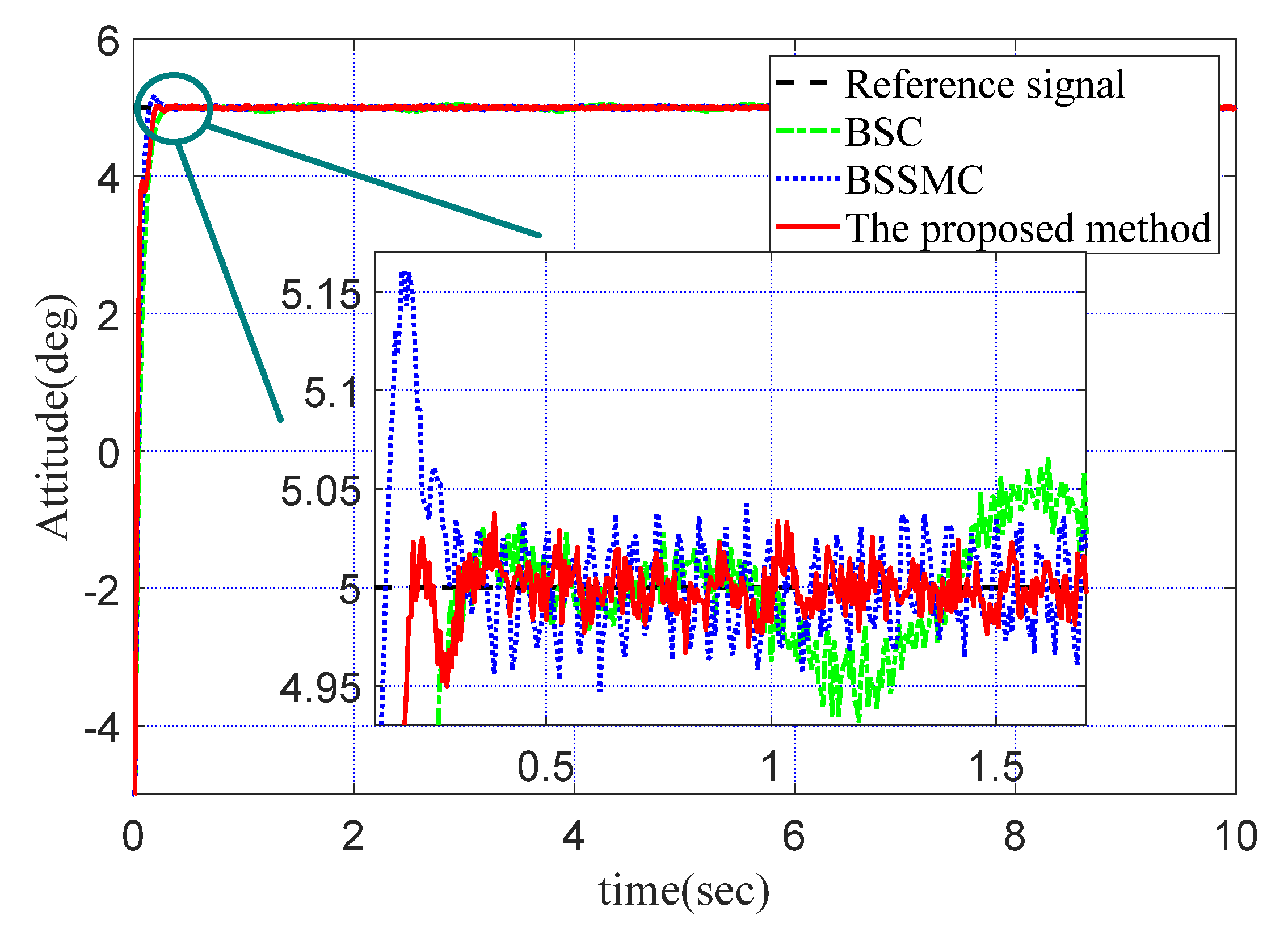
Figure 6 shows the comparison of the attitude angles generated by the three control methods. When the simulation time reaches 0.3 s, the attitude angles of the three control methods can all track the desired attitude angles, and there exists a peaking value in the initial stage of the BSSMC, which reaches 5.1609°. Compared with the other two control methods, the proposed control method has the best performance both in terms of response speed and robustness to disturbances, and the angle velocity of the proposed control method can reach $50°/\mathrm{s}$. In order to intuitively reflect the control performance of the three control methods, the root mean square error (RMSE), the integral of time-multiplied absolute-value of error (ITAE), and the maximum deviation of error (MAXE) are used as the performance indicators of the tracking error.

Table 2. The comparison of the control performances of the three control methods.

	RMSE	ITAE	MAXE
BS	0.0289	0.2204	0.0771
BSSMC	0.0210	0.1693	0.0541
The proposed method	0.0109	0.0831	0.0402
Improvements: BS	62.3%	62.3%	47.8%
Improvements: BSSMC	48.1%	51.0%	34.6%

shows the comparison of the control performances of the three control methods. It can be seen that the proposed control method has the best control performance under multiple disturbance environments. Compared with the BS and the BSSMC, the RMSE value, ITAE value, and MAXE value of the proposed method are improved by at least 48.1%, 51.0%, and 34.6%, respectively.

Figure 7 shows the comparison of the control voltages generated by the three control methods. Compared with the other two control methods, BSSMC has an obvious chattering problem, which is very disadvantageous to the actuator of the ISP system. The proposed control solves the chattering problem, and the peak voltage is only 1/4 of that of the BSSMC, which will keep the ISP system running longer.

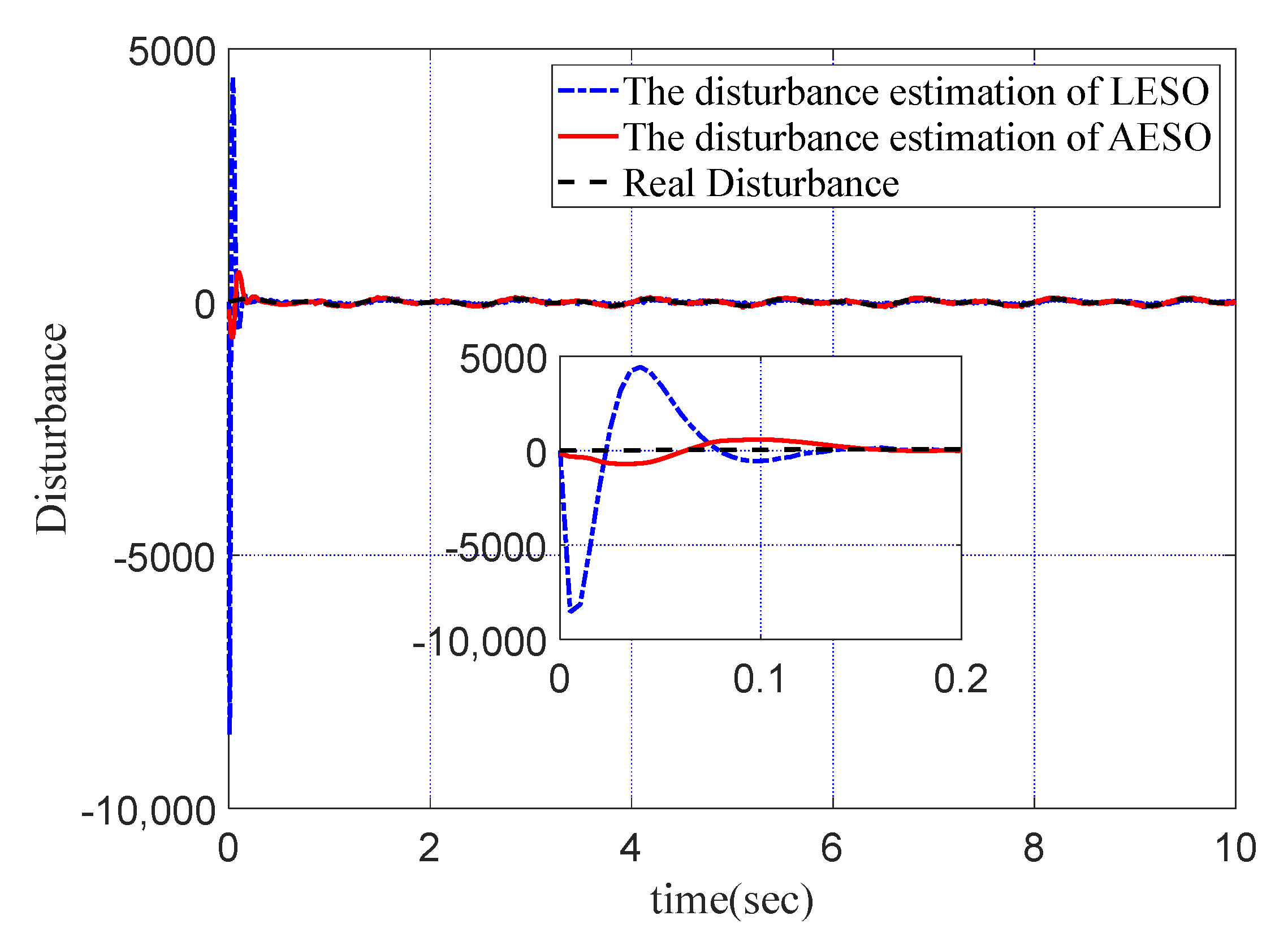
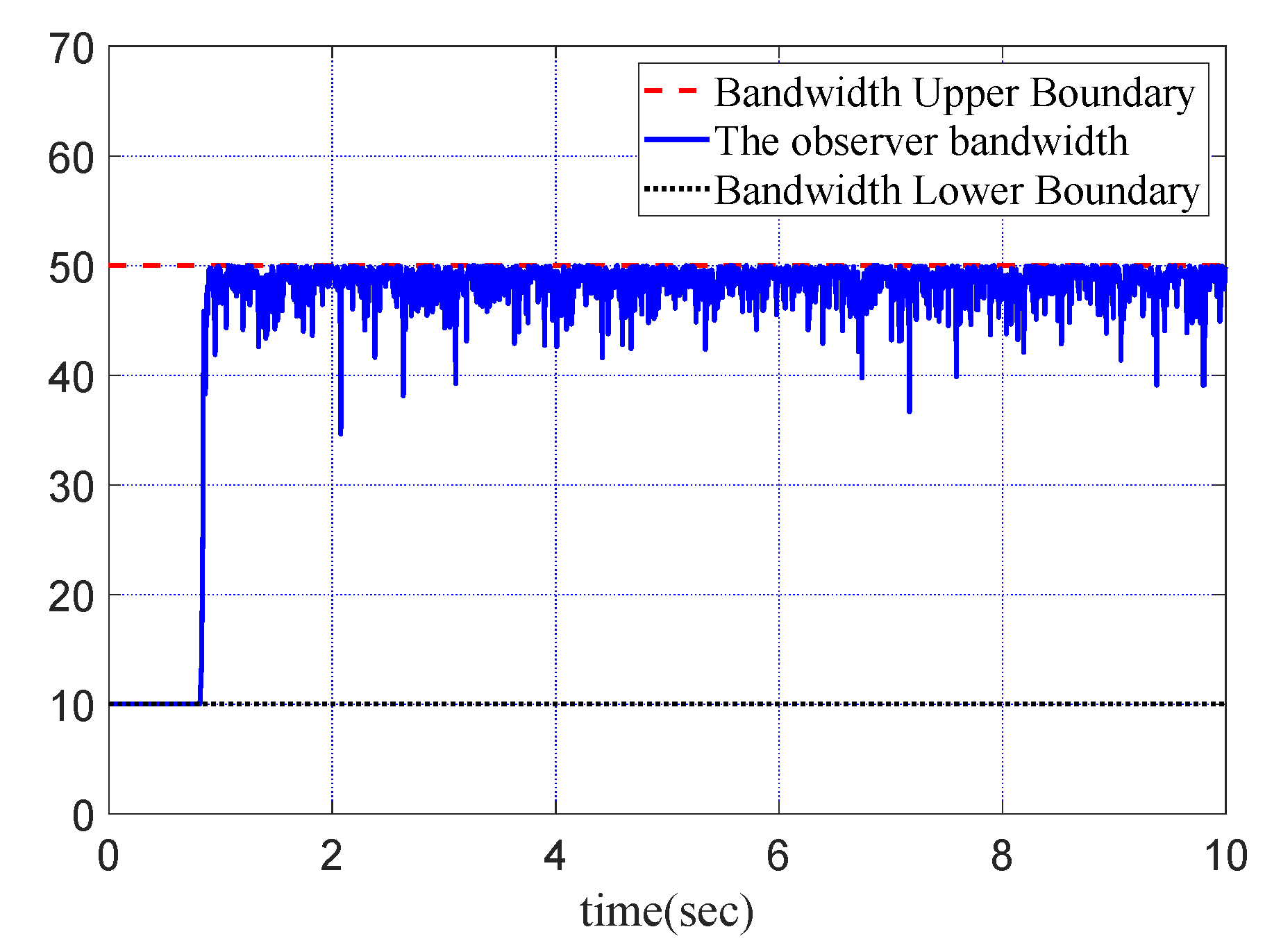
Figure 8, Figure 9 and Figure 10 show the simulation results for LESO and AESO. When the simulation time reaches 0.15 s, the disturbance estimations can track the real disturbance. Compared with LESO, there is no peaking phenomenon in AESO, and the disturbance estimation curve is more convergent. The maximum peak of estimation of AESO is only 8.09% of that of the LESO. In addition, the maximum disturbance estimation error of AESO is only 40% of that of the LESO. It can be seen from Figure 10 that the bandwidth variation of AESO guarantees the accuracy of AESO disturbance estimation.

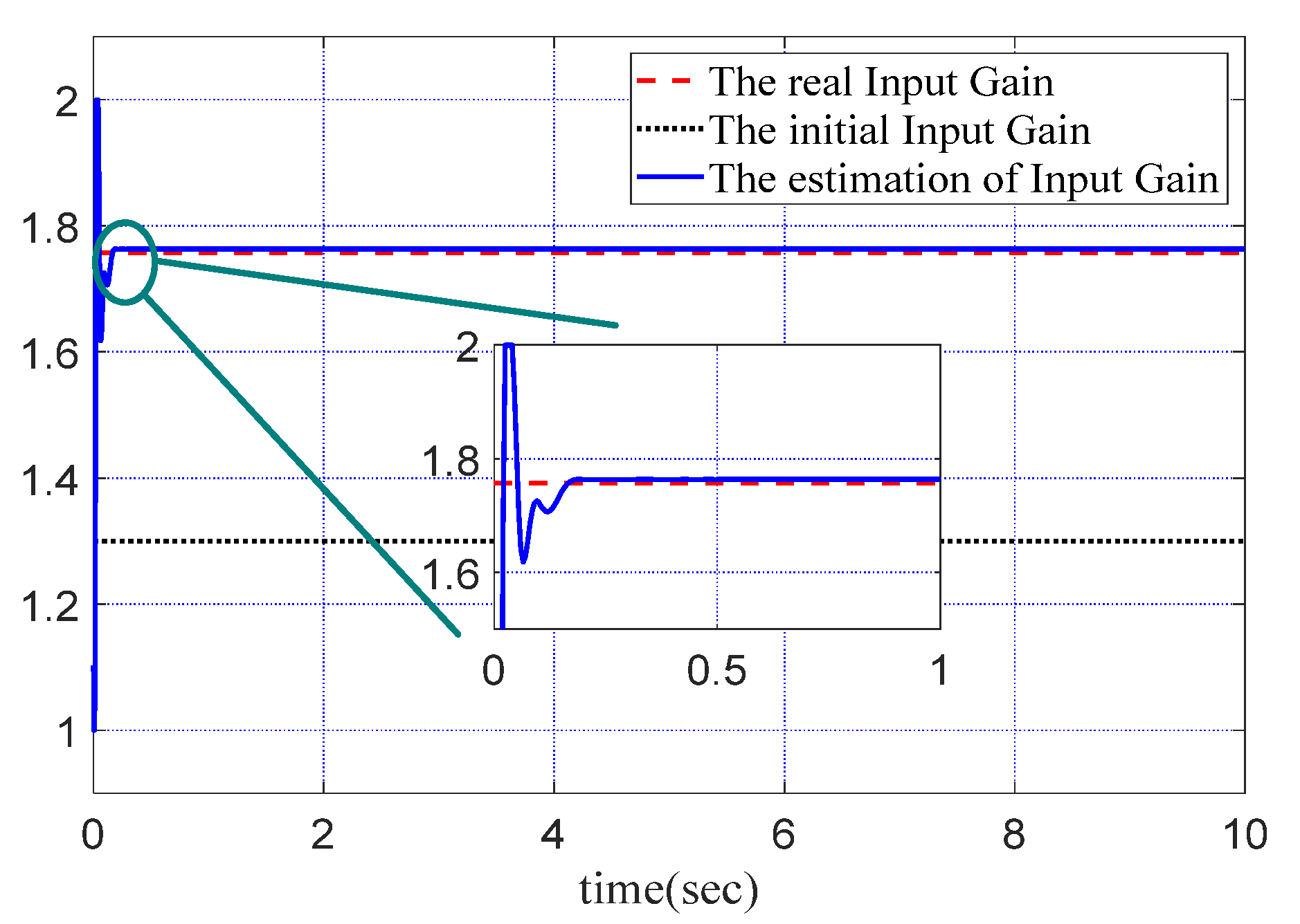
According to Figure 11, the estimation of input gain $\widehat{b}$ gradually approached the real input gain $b=1.7569$ with the parameter adaptation law $\widehat{J}$, and finally $\widehat{b}=1.7652$. Compared with the $b_0=1.3$, the parameter uncertainty of $\widehat{b}$ reduced by 98.2%, which greatly reduced the estimation burden of AESO.

4.2. Experiments

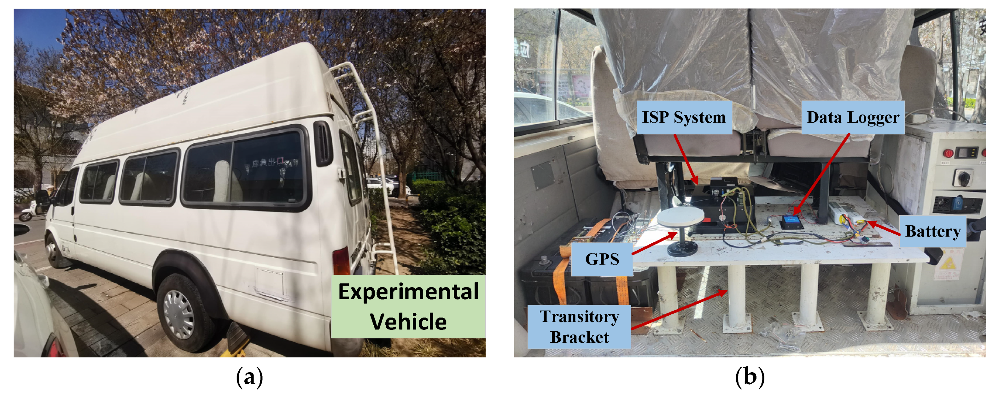
4.2.1. Case 1: Vehicle Experiment

To validate the control performance of the ISP system under the real disturbance environment, a vehicle experiment was carried out. The roll gimbal was chosen as an example, and let $x_{1d}=0°$. In order to verify the control performance of the proposed method, the adaptive neural network and sliding mode control (ANNSMC) method in [20] is also used in this part under the same experimental conditions. The parameters of the proposed method were set to the same as those used in the simulation.

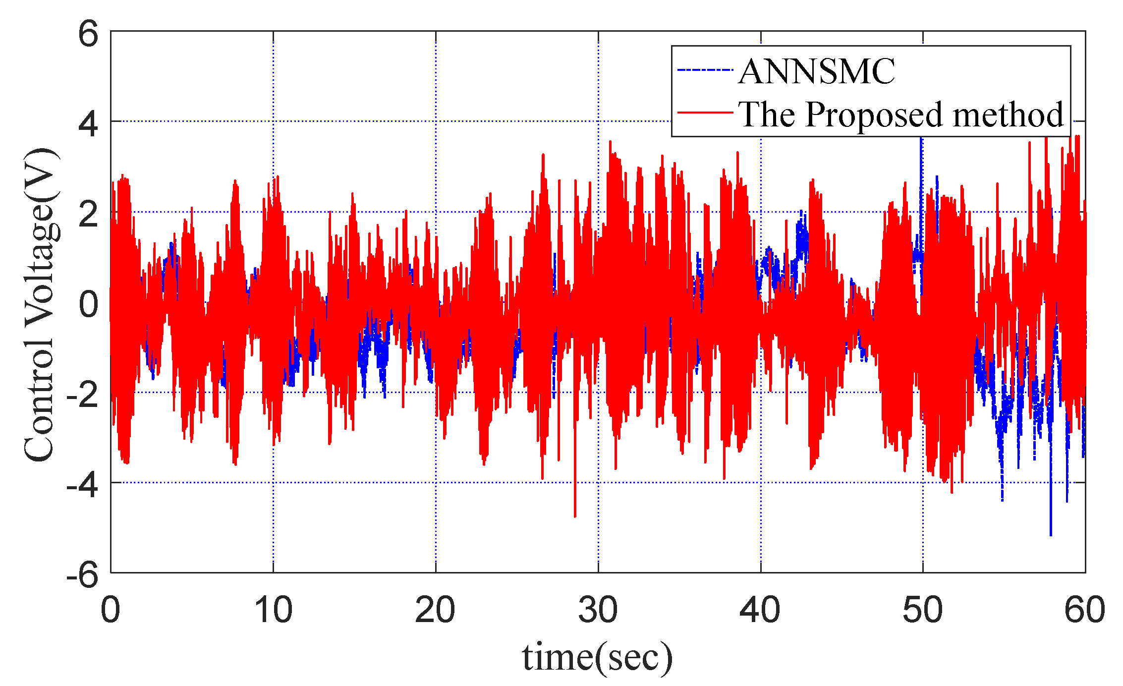
Figure 12 shows the experimental devices of the vehicle experiment. The ISP system was connected to the vehicle by the transitory bracket. The data logger was used to record the experimental data. Figure 13, Figure 14 and Figure 15 show the experimental results in the vehicle experiment. As can be seen from Figure 13, Figure 14 and Figure 15, both control methods can ensure the stable operation of the ISP system in the disturbance environment.

Table 3. The comparison of the control performances of the two control methods in the vehicle experiment.

	RMSE	ITAE	MAXE
ANNSMC	0.0939	4.1240	0.5278
The proposed method	0.0625	2.8966	0.2567
Improvements	33.4%	30.0%	51.4%

shows the comparison of the control performances of the two control methods in the vehicle experiment. It can be seen that the proposed control method has the best control performance in the vehicle experiment. Compared with the ANNSMC, the RMSE value, ITAE value, and MAXE value of the proposed method are improved by 33.4%, 30.0%, and 51.4%, respectively.

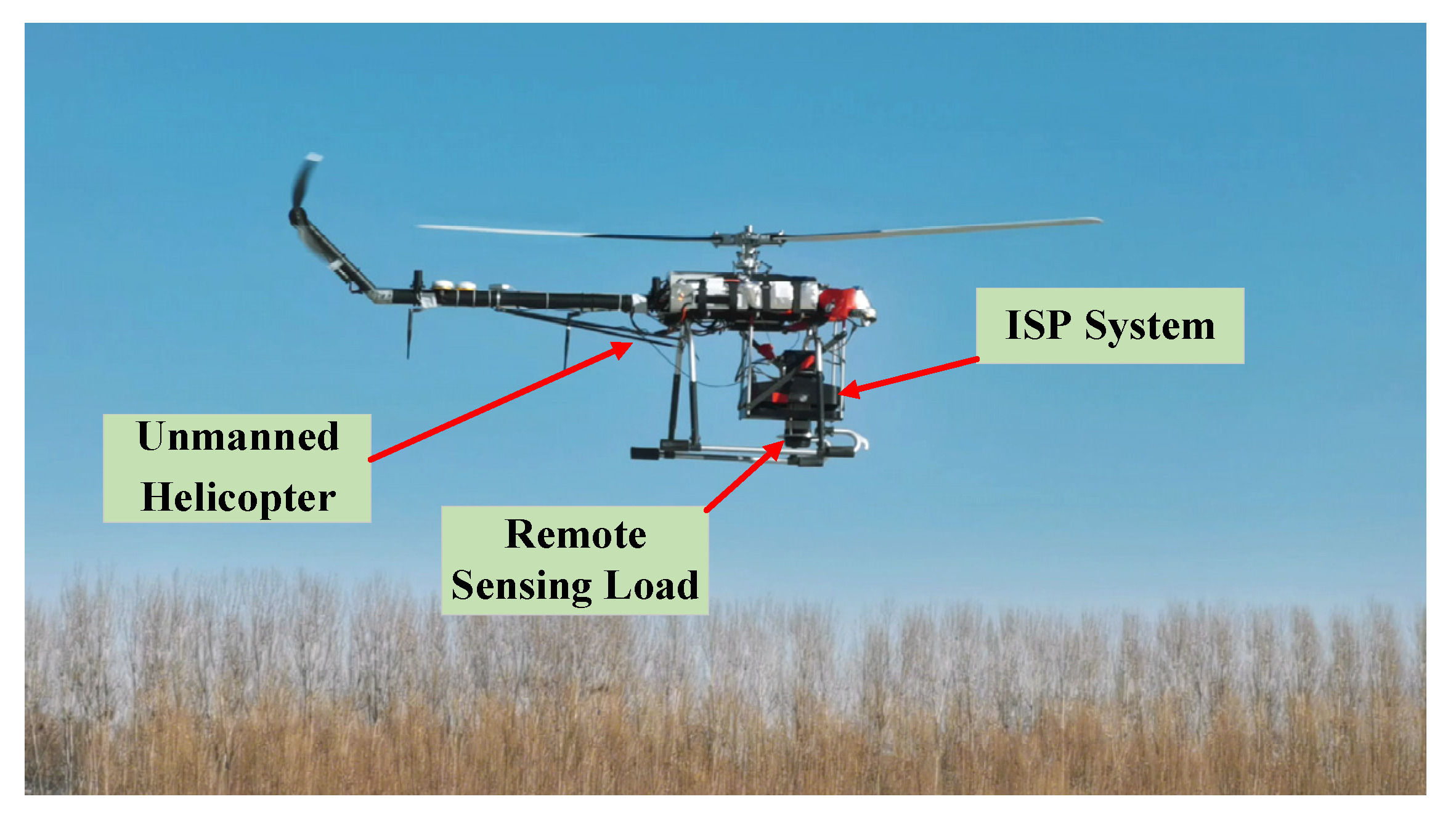
4.2.2. Case 2: Unmanned Helicopter Flight Experiment

To test the control performance of the proposed method in actual flight, a series of airport pavement inspections have been conducted in Tianjin city from August 2020 to February 2021. The unmanned helicopter inspection system is shown in Figure 16. Due to the consideration of counterweight, the ISP system was hung by four carbon fiber columns at the front abdomen of the unmanned helicopter.

With the consideration of camera index and the task requirement, the flight speed and flight height of the unmanned helicopter inspection system were set as 8 m/s and 20 m, respectively. Based on the MGNC system, the ISP adjusted the gimbals to keep the sight axis of load perpendicular to the ground, and the desired attitude angle ${\mathsf{\theta }}_d={\left[\begin{array}{ccc}{\theta }_{tpd}^p& {\theta }_{trd}^r& {\theta }_{tad}^a\end{array}\right]}^T$ was set to ${\left[\begin{array}{ccc}0°& 0°& 90°\end{array}\right]}^T$. 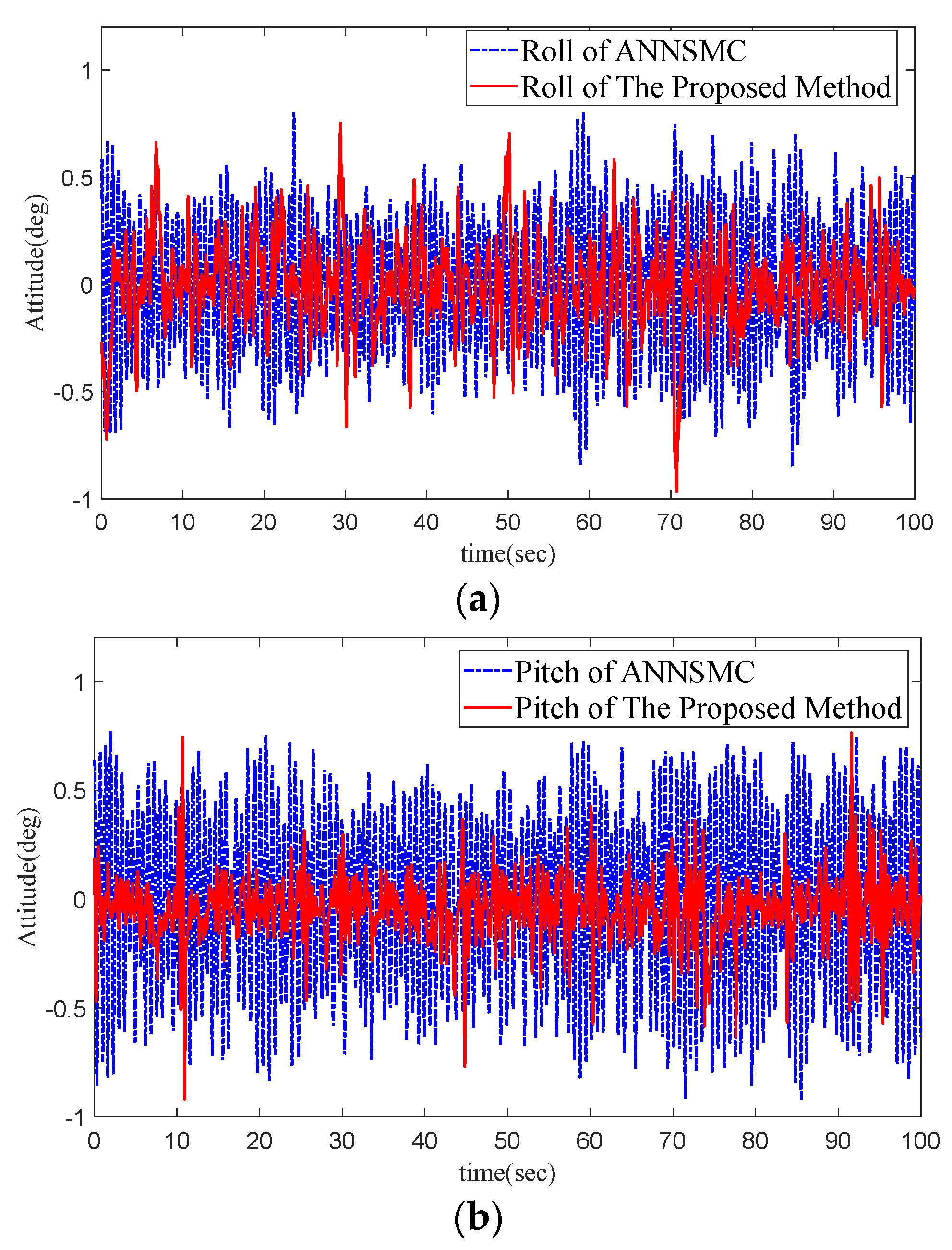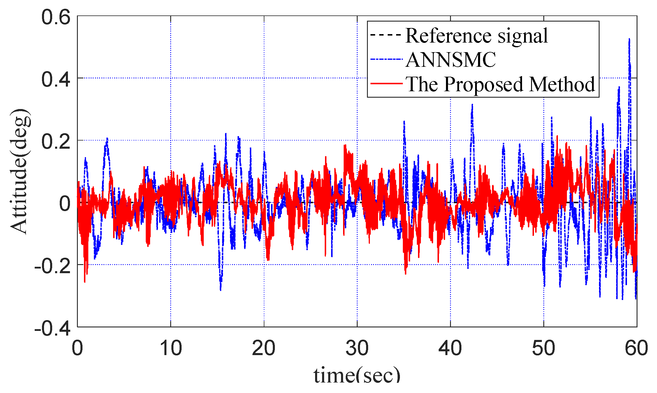Under the same flight experiment conditions, the same controllers were chosen as in Case 1. 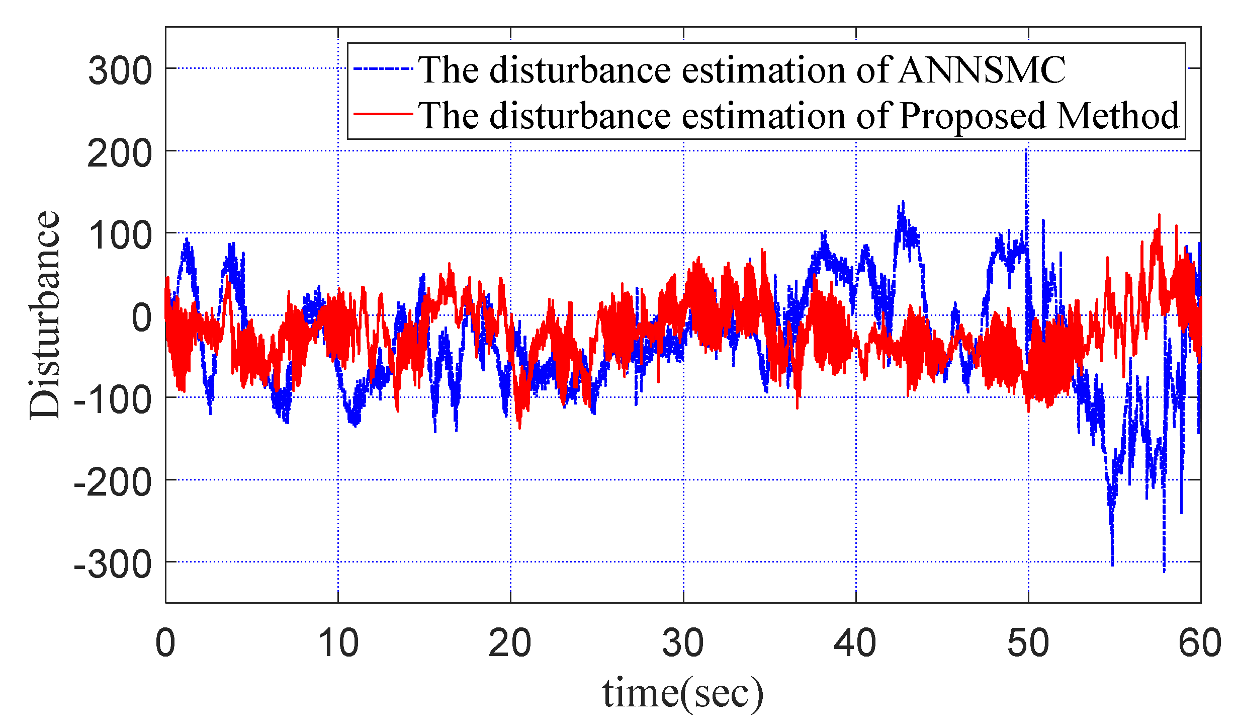The roll, pitch, and yaw angles of the ISP system generated by the proposed control method and ANNSMC are shown in Figure 17. Since the wind speed was 11.2 m/s, there were large wind disturbances in the flight test. The ISP could isolate non-ideal disturbances effectively to get high performance ground defect photos, and

Table 4. The comparison of the control performances of the two control methods in the flight experiment.

	Roll			Pitch			Yaw
	RMSE	ITAE	MAXE	RMSE	ITAE	MAXE	RMSE	ITAE	MAXE
ANNSMC	0.3121	26.7158	0.8489	0.3909	33.7795	0.9207	0.1126	7.0267	0.8317
The proposed method	0.2049	15.2741	0.9678	0.1479	10.6145	0.9174	0.0762	4.7119	0.5301
Improvements	34.3%	42.8%	−14.0%	62.2%	68.6%	0.36%	32.3%	32.9%	36.3%

shows the comparison of the control performances of the two control methods in the flight experiment.

As can be seen from Table 4, compared with the ANNSMC, the RMSE values and ITAE values of the proposed method are improved by at least 32.3% and 32.9%, respectively. However, the MAXE value of the roll gimbal of the proposed method is increased by 14.0%. Additionally, the MAXE values of the pitch gimbal and yaw gimbal of the proposed method are improved by 0.36% and 36.3%, respectively. Therefore, the proposed method has strong robustness against disturbances, which can achieve better control performance than ANNSMC.

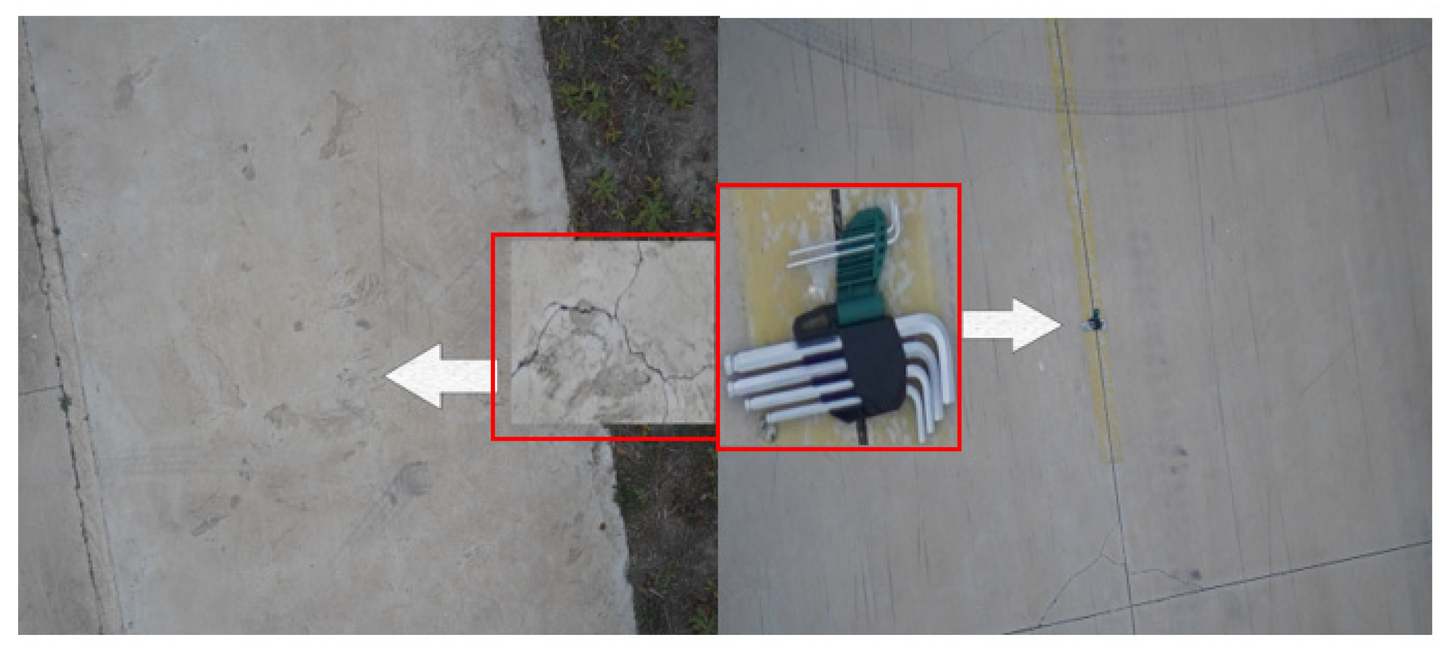
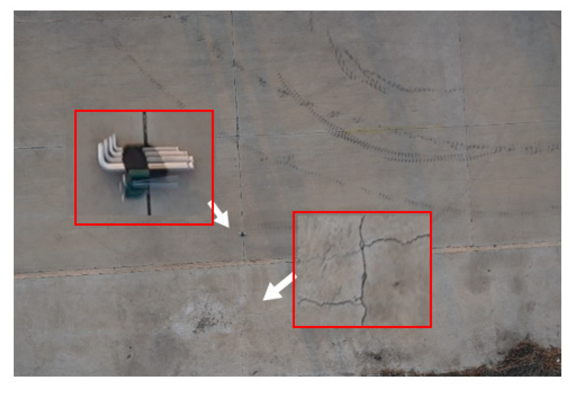
The inspection photos of the proposed method and ANNSMC are shown in Figure 18 and Figure 19. Compared with the ANNSMC, the 1 mm crack and 1.5 mm hexagon tool could be located in the photo of the proposed method clearly. The ISP system based on the proposed method could isolate different disturbances effectively to locate airport pavement diseases.

5. Conclusions

This paper proposed a nonlinear dynamic model based on the geographic coordinates and a compound control method based on the AESO and adaptive back-stepping integral SMC for the high-performance control of the three-axis ISP system. The dynamic model described in this paper can avoid complex coordinate transformation and improve the measurement and control performance. In the proposed compound control method, the adaptation laws based on the integral sliding mode for parameter uncertainty and disturbance estimation compensation are developed, which can improve the disturbance estimation accuracy of AESO. The chattering problem of SMC has been effectively reduced by introduction of lumped disturbance estimation. A series of simulation and experimental results show that the proposed control method can ensure high control precision for ISP under multiple disturbance environments. In our future work, the robustness of the proposed method will be discussed under various design parameters.

References

1. Masten, M.K. Inertially stabilized platforms for optical imaging systems. IEEE Control Syst. Mag. 2008, 28, 47–64. [Google Scholar]
2. Hilkert, J.M. Inertially stabilized platform technology Concepts and principles. IEEE Control Syst. Mag. 2008, 28, 26–46. [Google Scholar]
3. Zhou, X.; Zhang, H.; Yu, R. Decoupling control for two-axis inertially stabilized platform based on an inverse system and internal model control. Mechatronics 2014, 24, 1203–1213. [Google Scholar] [CrossRef]
4. Liu, S.; Che, H.; Sun, L. Research on stabilizing and tracking control system of tracking and sighting pod. J. Control Theory Appl. 2012, 10, 107–112. [Google Scholar] [CrossRef]
5. Fang, J.; Yin, R.; Lei, X. An adaptive decoupling control for three-axis gyro stabilized platform based on neural networks. Mechatronics 2015, 27, 38–46. [Google Scholar] [CrossRef]
6. Mu, Q.; Liu, G.; Lei, X. A RBFNN-Based Adaptive Disturbance Compensation Approach Applied to Magnetic Suspension Inertially Stabilized Platform. Math. Probl. Eng. 2014, 2014, 657985. [Google Scholar] [CrossRef]
7. Zhang, Y.; Yang, T.; Li, C.; Liu, S.; Du, C.; Li, M.; Sun, H. Fuzzy-PID control for the position loop of aerial inertially stabilized platform. Aerosp. Sci. Technol. 2014, 36, 21–26. [Google Scholar] [CrossRef]
8. Darestani, M.; Nikkhah, A.; Sedigh, A. H∞/Predictive output control of a three-axis gyrostabilized platform. Proc. Inst. Mech. Eng. IMechE Conf. 2013, 228, 679–689. [Google Scholar] [CrossRef]
9. Yu, Y.-J.; Fang, J.-C.; Xiang, B.; Wang, C.-E. Adaptive back-stepping tracking control for rotor shaft tilting of active magnetically suspended momentum wheel. ISA Trans. 2014, 53, 1892–1900. [Google Scholar] [CrossRef]
10. Setoodeh, P.; Khayatian, A.; Farjah, E. Backstepping-Based Control of a Strapdown Boatboard Camera Stabilizer. Int. J. Control Autom. Syst. 2007, 5, 15–23. [Google Scholar]
11. Guo, L.D.; Tan, Z.F.; Li, G.C.; Zhang, Q.T. Dynamic sliding-mode control with backstepping for stabilization loop of inertial platform. J. Chin. Inertial Technol. 2010, 18, 283–289. [Google Scholar]
12. Hou, S.; Chu, Y.; Fei, J. Intelligent Global Sliding Mode Control Using Recurrent Feature Selection Neural Network for Active Power Filter. IEEE Trans. Ind. Electron. 2021, 68, 7320–7329. [Google Scholar] [CrossRef]
13. Jiang, B.; Karimi, H.R.; Yang, S.; Gao, C.; Kao, Y. Observer-Based Adaptive Sliding Mode Control for Nonlinear Stochastic Markov Jump Systems via T–S Fuzzy Modeling: Applications to Robot Arm Model. IEEE Trans. Ind. Electron. 2021, 68, 466–477. [Google Scholar] [CrossRef]
14. Levant, A. High-order sliding modes: Differentiation and output feedback control. Int. J. Control 2003, 76, 427–434. [Google Scholar] [CrossRef]
15. Shtessel, Y.; Taleb, M.; Plestan, F. A novel adaptive-gain supertwisting sliding mode controller: Methodology and application. Automatica 2012, 48, 759–769. [Google Scholar] [CrossRef]
16. Mao, J.; Li, S.; Li, Q.; Yang, J. Design and implementation of continuous finite-time sliding mode control for 2-DOF inertially stabilized platform subject to multiple disturbances. ISA Trans. 2019, 84, 214–224. [Google Scholar] [CrossRef]
17. Mao, J.; Yang, J.; Li, S.; Yan, Y.; Li, Q. Output feedback-based sliding mode control for disturbed motion control systems via a higher-order ESO approach. IET Contr. Theory Appl. 2018, 12, 2118–2126. [Google Scholar] [CrossRef]
18. Lei, X.; Lu, P. The Adaptive Radial Basis Function Neural Network for Small Rotary-Wing Unmanned Aircraft. IEEE Trans. Ind. Electron. 2014, 61, 4808–4815. [Google Scholar] [CrossRef]
19. Giap, N.H.; Shin, J.-H.; Kim, W.-H. Robust Adaptive Neural Network Control for XY Table. Intell. Control Autom. 2013, 4, 293–300. [Google Scholar] [CrossRef]
20. Zou, Y.; Lei, X. A compound control method based on the adaptive neural network and sliding mode control for inertial stable platform. Neurocomputing 2015, 155, 286–294. [Google Scholar] [CrossRef]
21. Han, J. From PID to Active Disturbance Rejection Control. IEEE Trans. Ind. Electron. 2009, 56, 900–906. [Google Scholar] [CrossRef]
22. Liu, J.; Vazquez, S.; Wu, L.; Marquez, A.; Gao, H.; Franquelo, L.G. Extended State Observer-Based Sliding-Mode Control for Three-Phase Power Converters. IEEE Trans. Ind. Electron. 2017, 64, 22–31. [Google Scholar] [CrossRef]
23. Yao, J.; Jiao, Z.; Ma, D. Adaptive Robust Control of DC Motors With Extended State Observer. IEEE Trans. Ind. Electron. 2014, 61, 3630–3637. [Google Scholar] [CrossRef]
24. Sayem, A.H.M.; Cao, Z.; Man, Z. Model Free ESO-Based Repetitive Control for Rejecting Periodic and Aperiodic Disturbances. IEEE Trans. Ind. Electron. 2017, 64, 3433–3441. [Google Scholar] [CrossRef]
25. Ren, C.; Li, X.; Yang, X.; Ma, S. Extended State Observer-Based Sliding Mode Control of an Omnidirectional Mobile Robot with Friction Compensation. IEEE Trans. Ind. Electron. 2019, 66, 9480–9489. [Google Scholar] [CrossRef]
26. Pu, Z.; Yuan, R.; Yi, J.; Tan, X. A Class of Adaptive Extended State Observers for Nonlinear Disturbed Systems. IEEE Trans. Ind. Electron. 2015, 62, 5858–5869. [Google Scholar] [CrossRef]
27. Li, P.; Zhu, G.; Zhang, M. Linear Active Disturbance Rejection Control for Servo Motor Systems with Input Delay via Internal Model Control Rules. IEEE Trans. Ind. Electron. 2021, 68, 1077–1086. [Google Scholar] [CrossRef]
28. Yao, J.; Deng, W. Active Disturbance Rejection Adaptive Control of Hydraulic Servo Systems. IEEE Trans. Ind. Electron. 2017, 64, 8023–8032. [Google Scholar] [CrossRef]
29. Cheng, Y.; Ren, X.; Zheng, D.; Li, L. Non-Linear Bandwidth Extended-State-Observer Based Non-Smooth Funnel Control for Motor-Drive Servo Systems. IEEE Trans. Ind. Electron. 2022, 69, 6215–6224. [Google Scholar] [CrossRef]
30. Fu, F.; Lei, X.; Wang, R. A Compound Control Method Based on the Adaptive Linear Extended State Observer and Global Fast Terminal Sliding Mode Control for Inertially Stabilized Platform. Machines 2022, 10, 426. [Google Scholar] [CrossRef]
Figure 1. The schematic diagram of the three-axis ISP system.
Symmetry 14 01848 g001
Figure 2. Coordinates of the three-axis ISP system.
Symmetry 14 01848 g002
Figure 3. The flowchart of the compound method.
Symmetry 14 01848 g003
Figure 4. The frequency response of G D ( s ) .
Symmetry 14 01848 g004
Figure 5. The three-axis ISP.
Symmetry 14 01848 g005
Figure 6. The comparison of the attitude angles generated by the three control methods.
Symmetry 14 01848 g006
Figure 7. The comparison of the control voltages generated by the three control methods.
Symmetry 14 01848 g007
Figure 8. The comparison of the disturbance estimations generated by LESO and AESO.
Symmetry 14 01848 g008
Figure 9. The comparison of the disturbance estimations and errors generated by the LESO and AESO.
Symmetry 14 01848 g009
Figure 10. The observer bandwidth of AESO.
Symmetry 14 01848 g010
Figure 11. The estimation of input gain.
Symmetry 14 01848 g011
Figure 12. (a) Experimental vehicle (b) ISP system. Experimental devices for the vehicle experiment.
Symmetry 14 01848 g012
Figure 13. The comparison of the attitude angles generated by the two control methods of the vehicle experiment.
Symmetry 14 01848 g013
Figure 14. The comparison of the control voltages generated by the two control methods of the vehicle experiment.
Symmetry 14 01848 g014
Figure 15. The comparison of the disturbance estimations generated by the two control methods of the vehicle experiment.
Symmetry 14 01848 g015
Figure 16. Flight experiment system.
Symmetry 14 01848 g016
Figure 17. (a) Roll angle, (b) Pitch angle, (c) Yaw angle. The comparison of the attitude angles generated by the two control methods of the flight experiment.
Symmetry 14 01848 g017aSymmetry 14 01848 g017b
Figure 18. The inspection photos of the proposed method.
Symmetry 14 01848 g018
Figure 19. The inspection photos of ANNSMC.
Symmetry 14 01848 g019