Unified Representation of 3D Multivectors with Pauli Algebra in Rectangular, Cylindrical and Spherical Coordinate Systems

Abstract

In practical engineering, the use of Pauli algebra can provide a computational advantage, transforming conventional vector algebra to straightforward matrix manipulations. In this work, the Pauli matrices in cylindrical and spherical coordinates are reported for the first time and their use for representing a three-dimensional vector is discussed. This method leads to a unified representation for 3D multivectors with Pauli algebra. A significant advantage is that this approach provides a representation independent of the coordinate system, which does not exist in the conventional vector perspective. Additionally, the Pauli matrix representations of the nabla operator in the different coordinate systems are derived and discussed. Finally, an example on the radiation from a dipole is given to illustrate the advantages of the methodology.

1. Introduction

In 1865, Maxwell presented his treatise on the theory of electromagnetism (EM) [1]. However, what we generally denote as Maxwell’s equations (the four equations with divergence and curl) have never been written by Maxwell [1]. In fact, by using Hamiliton’s quaternions, in his treatise, Maxwell summarized the theory in a set of ten equations. At the beginning of 1900, by using symbolic vector calculus, Heaviside [2], along with Gibbs [3] and Helmholtz, reduced the system of ten equations in the well-known system of four equations as reported in modern books dealing with (EM) theory.

However, the scientific progress in the last century has proposed some considerable novelties. Around 1928, Wolfgang Pauli has introduced the representation of a vector in terms of a two-by-two matrix, thus allowing novel possible operations as, e.g., taking the inverse of a vector. In the same years, completely independently, Paul A. M. Dirac has introduced the Dirac matrices in order to express the Dirac equation [4,5]. In addition, in the last century, the contributions of Hamilton, Grassmann, Clifford and others have been clarified and better understood [6].

In fact, it has been recognized that both Pauli and Dirac algebras can be related to the Clifford algebra [7], often referred to also as Geometric Algebra (GA). The description of the space in terms of GA is considerably more satisfying than traditional vector analysis. In fact, in vector analysis, there are only scalars (points) and vectors. In addition, vector analysis does not represent an algebra and therefore a plethora of different rules have to be followed for performing various tasks. Conventional vector analysis only holds true in the three-dimensional space, while GA can be used in whatever number of dimensions. In particular, according to GA, elements in a three–dimensional space can be represented by using a multivector, which is the sum of a scalar (i.e., a point), a vector (i.e., an oriented line), a bivector (i.e., an oriented surface) and a trivector or pseudoscalar (i.e., a volume element). In three dimensions, it is possible to multiply multivectors as simply as we can multiply two-by-two matrices. Such 3D multivectors can be represented by two-by-two Pauli matrices. According to these considerations, in recent years, the interest on the application of geometric algebra has grown significantly and many excellent books have appeared [8,9,10,11,12,13,14].

Recently, a plethora of GA applications has arisen [15,16], spreading over different disciplines, such as signal and image processing [17], artificial intelligence [18], robotics [19] and molecular geometry [20]. Its application potential is not surprising. Indeed, whenever Euclidean transformations are present, the issue can be expressed in terms of GA. In particular, with regard to EM problems, an excellent introduction to GA and the related advantages has been provided in [21]. It is shown that Maxwell equations can be grouped into a single equation [6,22] or can be expressed in a compact form similar to the Dirac equation for null mass [23].

In this paper, assuming that the reader is familiar with GA, the advantages related to the use of Pauli matrices are highlighted for engineering purposes. While Clifford algebra or GA are very nice for a theoretical framework, in practical engineering computations, the use of Pauli matrices provides a significant advantage. In fact, they are very suitable for introduction in a Computer Algebra System (CAS). As a matter of fact, modern CAS allow for developing the required vector algebra entirely at the computer level, so that tedious computations can be avoided. In this paper, the Pauli matrices in cylindrical and spherical coordinates are reported for the first time and their use for representing a three-dimensional vector is discussed. They provide a representation which is independent of the coordinate system, which does not exist in the conventional vector approach. Additionally, the Pauli matrix representation of the nabla operator ∇ is introduced and discussed.

The paper is structured as follows: first, the multivector representation via Pauli vectors is introduced (Section 2). Next, the Pauli matrices in rectangular coordinates are converted to cylindrical and spherical coordinates in Section 3. In addition, the ∇ operator can be expressed in rectangular, cylindrical and spherical coordinates by using Pauli matrices as demonstrated in Section 4. Finally, the results are applied on a dipole as example (Section 5).

2. Multivector Representation via Pauli Matrices

In this section, first, the conventional representation of vectors is recalled and some drawbacks are highlighted. Next, a Clifford algebra vector representation is recollected to overcome these disadvantages. Finally, the well known Pauli matrices in rectangular coordinates and Pauli vectors are introduced and discussed.

2.1. Conventional Representation of Vectors

Three–dimensional vectors are usually represented as three ordered numbers, e.g., $\mathbf{a}={\left(a_x,a_y,a_z\right)}^T$. Vectors are generally represented in the rectangular, cylindrical and spherical coordinate systems as

$$\begin{array}{ccc}\hfill \mathbf{A}& =& A_x{\mathbf{x}}_0+A_y{\mathbf{y}}_0+A_z{\mathbf{z}}_0\hfill \\ & =& A_{\rho }{\mathbf{u}}_{\rho }+A_{\varphi }{\mathbf{u}}_{\varphi }+A_z{\mathbf{u}}_z\hfill \\ & =& A_r{\mathbf{u}}_r+A_{\theta }{\mathbf{u}}_{\theta }+A_{\varphi }{\mathbf{u}}_{\varphi }.\hfill \end{array}$$

(1)

Different conventions exist for representing the coordinates of a spherical coordinate system. In this work, the convention usually applied in physics is used, specified by the ISO standard 80000-2:2019. The right-handed coordinate system $({\mathbf{u}}_r,{\mathbf{u}}_{\theta },{\mathbf{u}}_{\varphi })$ is applied, with ${\mathbf{u}}_{\theta }$ the inclination unit vector (corresponding to the angle with respect to the polar axis) and ${\mathbf{u}}_{\varphi }$ referring to the azimuthal angle (Figure 1).

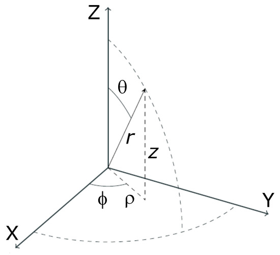
Figure 1. Convention for the rectangular $(x,y,z)$, cylindrical $(\rho ,\varphi ,z)$ and spherical $(r,\theta ,\varphi )$ coordinate systems.

The representation in (1), which is based on the use of unit vectors, has several drawbacks:

• vectors cannot be multiplied;
• it is not possible to find the inverse;
• given two vectors $\mathbf{a}$ and $\mathbf{b}$, it is not possible to find the transformation which leads from $\mathbf{a}$ to $\mathbf{b}$,
• the cross product of vectors is misleading; instead a bivector, which is an oriented surface, should be used,
• no volume elements are present,
• it depends on the coordinate system.

As demonstrated in [21], the use of a Clifford algebra $Cl (3,0)$, recalled in the next section, allows for overcoming these issues.

2.2. Clifford Algebra of the Three-Dimensional Space

In a Clifford algebra $Cl (3,0)$, a vector is represented as follows:

$$\mathbf{A}=A_1{\mathbf{e}}_1+A_2{\mathbf{e}}_2+A_3{\mathbf{e}}_3.$$

(2)

The basis elements ${\mathbf{e}}_1$, ${\mathbf{e}}_2$ and ${\mathbf{e}}_3$ form an orthonormal basis for the vector space ${\mathbb{R}}^n$. In order to establish a Clifford algebra $Cl (3,0)$, ${\mathbf{e}}_1$, ${\mathbf{e}}_2$ and ${\mathbf{e}}_3$ have to satisfy the following conditions for $i=1,2,3$:

$${\mathbf{e}}_i^2=1$$

(3)

$${\mathbf{e}}_i{\mathbf{e}}_j=-{\mathbf{e}}_j{\mathbf{e}}_i,(i\ne j).$$

(4)

By using the correspondence shown in Table 1, Equation (2) can be used to refer to all the three coordinate systems.

Table 1. Vector $\mathbf{A}$ equivalence for rectangular, cylindrical and spherical coordinate systems.

	${\mathit{A}}_1$	${\mathit{A}}_2$	${\mathit{A}}_3$
Rectangular	$A_x$	$A_y$	$A_z$
Cylindrical	$A_{\rho }$	$A_{\varphi }$	$A_z$
Spherical	$A_r$	$A_{\theta }$	$A_{\varphi }$

However, there is also another possible representation in terms of 2 × 2 matrices. Naturally, a 2 × 2 real matrix is defined by four numbers, while a complex one requires eight numbers. It is therefore fairly natural that it is possible to represent a vector via a matrix. However, there are many possible representations, but, among them, the representation introduced by Wolfgang Pauli has several advantages. In the next section, the Pauli matrices in rectangular coordinates will be introduced, and their properties will be discussed. They are related to the Clifford’s algebra, and they satisfy (3) and (4). Accordingly, the representation of a vector in terms of Pauli matrices provides the same advantages of a Clifford’s algebra. Some instructive relationships between conventional vector analysis and GA are given in Appendix A.

2.3. Pauli Matrices in Rectangular Coordinates

In rectangular coordinates, the Pauli matrices have the following form:

$$\begin{array}{ccc}\hfill {\sigma }_1& =& \left(\begin{array}{cc}0& 1\\ 1& 0\end{array}\right)\hfill \\ \hfill {\sigma }_2& =& \left(\begin{array}{cc}0& -i\\ i& 0\end{array}\right)\hfill \\ \hfill {\sigma }_3& =& \left(\begin{array}{cc}1& 0\\ 0& -1\end{array}\right).\hfill \end{array}$$

(5)

Notice that the trace of the Pauli matrices is zero, and their determinant is −1. The square of the Pauli matrices equals the identity matrix I:

$${\sigma }_1^2={\sigma }_2^2={\sigma }_3^2=\left(\begin{array}{cc}1& 0\\ 0& 1\end{array}\right)=I={\sigma }_0.$$

(6)

By multiplying, e.g., ${\sigma }_1$ with ${\sigma }_2$, the result is $i{\sigma }_3$ and similar for the other cases:

$$\begin{array}{ccc}\hfill {\sigma }_1{\sigma }_2& =& i{\sigma }_3=-{\sigma }_2{\sigma }_1\hfill \\ \hfill {\sigma }_2{\sigma }_3& =& i{\sigma }_1=-{\sigma }_3{\sigma }_2\hfill \\ \hfill {\sigma }_3{\sigma }_1& =& i{\sigma }_2=-{\sigma }_1{\sigma }_3.\hfill \end{array}$$

(7)

The above relations are very important. In fact, they show that, in the three-dimensional case, it is always possible to replace the quantities ${\sigma }_i{\sigma }_j$ with the orthogonal vector $i{\sigma }_k$ (with the appropriate combination given in (7)). An equivalent property is also present in the Clifford algebra. Let us first note that, for the trivector $e_{123}$, it applies that:

$$e_{123}{e}_{123}=-1$$

(8)

and therefore $e_{123}=i$. In fact, if we consider the bivectors ${\mathbf{e}}_{12},{\mathbf{e}}_{13},{\mathbf{e}}_{23}$ and multiply them by $-i^2=1=-i{e}_{123}$, we have

$$\begin{array}{ccc}\hfill {\mathbf{e}}_{12}=-i{e}_{123}{\mathbf{e}}_{12}& =& i{\mathbf{e}}_3\hfill \\ \hfill {\mathbf{e}}_{13}=-i{e}_{123}{\mathbf{e}}_{13}& =& -i{\mathbf{e}}_2\hfill \\ \hfill {\mathbf{e}}_{23}=-i{e}_{123}{\mathbf{e}}_{23}& =& i{\mathbf{e}}_1.\hfill \end{array}$$

(9)

From the above properties, it is seen that, similarly for the Clifford basis, we have

$${\left({\sigma }_1{\sigma }_2{\sigma }_3\right)}^2={\sigma }_1{\sigma }_2{\sigma }_3{\sigma }_1{\sigma }_2{\sigma }_3=-1{\sigma }_0=-{\sigma }_0$$

(10)

i.e.,

$${\sigma }_1{\sigma }_2{\sigma }_3=i{\sigma }_0.$$

(11)

The three Pauli matrices and the identity matrix ${\sigma }_0$ constitute a basis in the space of two-by-two Hermitian matrices. A matrix A can be written as:

$$A=a_0{\sigma }_0+a_1{\sigma }_1+a_2{\sigma }_2+a_3{\sigma }_3.$$

(12)

It is worthwhile to note that, when the coefficients ($a_0,a_1,a_2,a_3$) are complex, non Hermitian matrices can also be described by the basis of (${\sigma }_0,{\sigma }_1,{\sigma }_2,{\sigma }_3$).

2.4. The Pauli Vector

2.4.1. Definition

The Pauli vector is a vector constructed by using the three matrices (${\sigma }_1,{\sigma }_2,{\sigma }_3$) as follows:

$$\sigma =\left({\sigma }_1{\mathbf{x}}_0+{\sigma }_2{\mathbf{y}}_0+{\sigma }_3{\mathbf{z}}_0\right)$$

(13)

with ${\mathbf{x}}_0$, ${\mathbf{y}}_0$ and ${\mathbf{z}}_0$ orthonormal basis unit vectors.

For a vector $\mathbf{a}=\left(a_x{\mathbf{x}}_0+a_y{\mathbf{y}}_0+a_z{\mathbf{z}}_0\right)$ in the three-dimensional space, the matrix $\tilde{a}$ is defined as the following product:

$$\tilde{a}\equiv \sigma ·\mathbf{a}=\left(\begin{array}{cc}{a}_z& a_x-i{a}_y\\ a_x+i{a}_y& -a_z\end{array}\right).$$

(14)

The vector $\mathbf{a}$ can be expressed as a two-by-two matrix $\tilde{a}$. The standard vector representation $\mathbf{a}$ and the matrix $\tilde{a}$ represent the same quantity, and it is always possible to pass from one to the other.

The inner product of two matrices $\tilde{a},\tilde{b}$, not necessarily representing vectors, is defined as

$$⟨\tilde{a},\tilde{b}⟩=\frac{1}{2}trace\left(\tilde{a}·\tilde{b}\right).$$

(15)

From the properties of the Pauli matrices, it can be easily verified that:

• for $i\ne j$, $⟨{\sigma }_i,{\sigma }_j⟩=0$,
• $⟨{\sigma }_i,{\sigma }_i⟩=1$.

Referring to (12), this provides a simple way to retrieve the coefficients of the Pauli matrices for a given matrix A:

$$⟨A,{\sigma }_0⟩=a_0⟨{\sigma }_0,{\sigma }_0⟩+a_1⟨{\sigma }_1,{\sigma }_0⟩+a_2⟨{\sigma }_2,{\sigma }_0⟩+a_3⟨{\sigma }_3,{\sigma }_0⟩=a_0$$

(16)

and similarly for the other components.

2.4.2. Space Description

It is noted that elements in three-dimensional space are described by eight numbers (i.e., a complex 2 × 2 matrix). In particular, they are

• one scalar (${\sigma }_0$): grade 0;
• 3 basis vectors (${\sigma }_1,{\sigma }_2,{\sigma }_3$) corresponding to three directions: grade 1;
• 3 basis bivectors (${\sigma }_1{\sigma }_2,{\sigma }_1{\sigma }_3,{\sigma }_2{\sigma }_3$): grade 2;
• one pseudoscalar ($i{\sigma }_0$): grade 3.

All these elements are contained in a matrix and, similarly to what we do for complex numbers, they can be written together in a multivector $\mathit{M}$ as

$$\mathit{M}=a_0+\mathbf{a}+\widehat{\mathbf{B}}+\widehat{\mathit{t}}$$

(17)

where $a_0$ is a scalar, $\mathbf{a}$ is a vector, $\widehat{\mathbf{B}}$ is a bivector and $\widehat{\mathit{t}}$ is a pseudoscalar.

We have started this section showing that a vector can be represented by a Pauli matrix. It is now possible to conclude that, in the three–dimensional space, a Pauli matrix not only can represent a vector, but it can encode all the information of the eight-dimensional base of a multivector! In other words, a multivector can be represented as a Pauli matrix, which will be illustrated next. Note that, since matrix algebra is well-known, we can also multiply, take the inverse, etc. of multivectors with ease.

2.4.3. Pauli Matrix Representation of a Multivector

Let us see with more details the Pauli matrix representation of a multivector. The corresponding matrices of the multivector in (17) are given next:

$$\begin{array}{ccc}\hfill \widetilde{a_0}& =& \left(\begin{array}{cc}{a}_0& 0\\ 0& a_0\end{array}\right)\hfill \\ \hfill \tilde{a}& =& \left(\begin{array}{cc}{a}_3& a_1-i{a}_2\\ i{a}_2+a_1& -a_3\end{array}\right)\hfill \\ \hfill \tilde{B}& =& \left(\begin{array}{cc}i{B}_3& B_2+i{B}_1\\ i{B}_1-B_2& -i{B}_3\end{array}\right)\hfill \\ \hfill \tilde{t}& =& \left(\begin{array}{cc}it& 0\\ 0& it\end{array}\right).\hfill \end{array}$$

(18)

The matrices in (18) can be summed together giving, for the multivector $\mathit{M}$,

$$\tilde{\mathit{M}}=\left(\begin{array}{cc}i{B}_3+it+a_3+a_0& B_2+i{B}_1-i{a}_2+a_1\\ -B_2+i{B}_1+i{a}_2+a_1& -i{B}_3+it-a_3+a_0\end{array}\right).$$

(19)

For a given Pauli matrix, it is possible to retrieve the elements of the different grades as described next.

2.4.4. Retrieving the Elements of a Multivector

Let us assume that the matrix in (19) is given, and we want to retrieve the various elements. It is convenient to extract the real and imaginary part of $\tilde{\mathit{M}}$ as

$$\begin{array}{ccc}\hfill \widetilde{M_r}& =& \mathrm{R}\mathrm{e}\left\{\mathit{M}\right\}=\left(\begin{array}{cc}{a}_3+a_0& B_2+a_1\\ a_1-B_2& a_0-a_3\end{array}\right)\hfill \\ \hfill \widetilde{M_i}& =& \mathrm{I}\mathrm{m}\left\{\mathit{M}\right\}=\left(\begin{array}{cc}{B}_3+t& B_1-a_2\\ B_1+a_2& t-B_3\end{array}\right).\hfill \end{array}$$

(20)

By inspection, it is seen that we have the following identities that express the different elements of the multivector:

$$\begin{array}{ccc}\hfill a_0& =& \frac{1}{2}\left({\widetilde{M_r}}_{11}+{\widetilde{M_r}}_{22}\right)\hfill \\ \hfill a_1& =& \frac{1}{2}\left({\widetilde{M_r}}_{12}+{\widetilde{M_r}}_{21}\right)\hfill \\ \hfill a_2& =& \frac{1}{2}\left({\widetilde{M_i}}_{21}-{\widetilde{M_i}}_{12}\right)\hfill \\ \hfill a_3& =& \frac{1}{2}\left({\widetilde{M_r}}_{11}-{\widetilde{M_r}}_{22}\right)\hfill \\ \hfill B_1& =& \frac{1}{2}\left({\widetilde{M_i}}_{21}+{\widetilde{M_i}}_{12}\right)\hfill \\ \hfill B_2& =& \frac{1}{2}\left({\widetilde{M_r}}_{12}-{\widetilde{M_r}}_{21}\right)\hfill \\ \hfill B_3& =& \frac{1}{2}\left({\widetilde{M_i}}_{11}-{\widetilde{M_i}}_{22}\right)\hfill \\ \hfill t& =& \frac{1}{2}\left({\widetilde{M_i}}_{11}+{\widetilde{M_i}}_{22}\right).\hfill \end{array}$$

(21)

3. Pauli Matrices in Different Coordinate Systems

The Pauli matrices in rectangular coordinates and their properties have been introduced in Section 2. In this section, their expressions in cylindrical and spherical coordinates are derived by two different methods: first by applying the transformation equations, and next by rotations.

3.1. Pauli Matrices in Cylindrical Coordinates

For the rectangular coordinate system, the Pauli matrices are ${\sigma }_i$, with $i=1,2,3$. When expressing a vector, it is possible to identify ${\sigma }_1$ with ${\mathbf{u}}_x$, ${\sigma }_2$ with ${\mathbf{u}}_y$ and ${\sigma }_3$ with ${\mathbf{u}}_z$.

Consider the unit vectors $({\mathbf{u}}_{\rho },{\mathbf{u}}_{\varphi },{\mathbf{u}}_z)$ of a cylindrical coordinate system. By using the equations for transforming the rectangular coordinates into the cylindrical ones, it is possible to write for the radial unit vector:

$${\mathbf{u}}_{\rho }={\mathbf{u}}_{x}cos\varphi +{\mathbf{u}}_{y}sin\varphi$$

(22)

resulting in the corresponding Pauli matrix:

$$\begin{array}{ccc}\hfill {\sigma }_{\rho }& =& cos\varphi {\sigma }_1+sin\varphi {\sigma }_2\hfill \\ & =& \left(\begin{array}{cc}0& e^{-i\varphi }\\ e^{i\varphi }& 0\end{array}\right).\hfill \end{array}$$

(23)

Similarly, it applies that:

$${\mathbf{u}}_{\varphi }=-{\mathbf{u}}_{x}sin\varphi +{\mathbf{u}}_{y}cos\varphi$$

(24)

from which the following Pauli matrix follows:

$$\begin{array}{ccc}\hfill {\sigma }_{\varphi }& =& -sin\varphi {\sigma }_1+cos\varphi {\sigma }_2\hfill \\ & =& \left(\begin{array}{cc}0& -i{e}^{-i\varphi }\\ i{e}^{i\varphi }& 0\end{array}\right).\hfill \end{array}$$

(25)

Naturally, for the vertical z component, the relation is that ${\sigma }_z={\sigma }_3$.

While in rectangular coordinates the Pauli matrices are not dependent on the coordinate, for the cylindrical coordinates, it is noted that ${\sigma }_{\rho }$ and ${\sigma }_{\varphi }$ are dependent on $\varphi$. For the derivatives with respect to $\varphi$, it applies that, with the abbreviated notation ${\partial }_{\varphi }=\partial /\partial \varphi$,

$$\begin{array}{ccc}\hfill {\partial }_{\varphi }{\sigma }_{\rho }& =& {\sigma }_{\varphi }\hfill \\ \hfill {\partial }_{\varphi }{\sigma }_{\varphi }& =& -{\sigma }_{\rho }.\hfill \end{array}$$

(26)

It is readily proved that the matrices ${\sigma }_{\rho },{\sigma }_{\varphi },{\sigma }_z$ when multiplied by themselves give the identity matrix ${\sigma }_0$, their trace is null, their determinant is always $-1$ and their dot product is zero if they are not the same. In addition, we have

$$\begin{array}{ccc}\hfill i{\sigma }_z& =& {\sigma }_{\rho }{\sigma }_{\varphi }\hfill \\ \hfill i{\sigma }_{\rho }& =& {\sigma }_{\varphi }{\sigma }_z\hfill \\ \hfill i{\sigma }_{\varphi }& =& {\sigma }_z{\sigma }_{\rho }.\hfill \end{array}$$

(27)

Therefore, the generic vector $\mathbf{A}$ can be expressed in cylindrical coordinates in terms of Pauli matrices as

$$\begin{array}{ccc}\hfill \tilde{A}& =& A_{\rho }{\sigma }_{\rho }+A_{\varphi }{\sigma }_{\varphi }+A_z{\sigma }_z\hfill \\ & =& \left(\begin{array}{cc}{A}_z& e^{-i\varphi }\left(A_{\rho }-i{A}_{\varphi }\right)\\ e^{i\varphi }\left(A_{\rho }+i{A}_{\varphi }\right)& -A_z\end{array}\right).\hfill \end{array}$$

(28)

By performing the inner product of the above expression with a selected sigma matrix, it is possible to recover the desired component in terms of the other basis. Thus, all the transformation between vectors in different coordinate systems can be simply obtained by matrix multiplication and trace operation. As an example, the expression of $A_{\rho }$ in terms of the rectangular components can be calculated by performing the inner product of both sides of (28) times ${\sigma }_{\rho }$:

$$\begin{array}{ccc}\hfill A_{\rho }& =& A_x{\sigma }_1·{\sigma }_{\rho }+A_y{\sigma }_2·{\sigma }_{\rho }+A_z{\sigma }_3·{\sigma }_{\rho }\hfill \\ & =& {A_{x}cos\varphi +A}_{y}sin\varphi \hfill \end{array}$$

(29)

where the inner product corresponds to making the matrix product and taking half of the trace.

3.2. Pauli Matrices in Spherical Coordinates

The procedure to derive the Pauli matrices in spherical coordinates is the same adopted for the cylindrical coordinate system. Consider the unit vectors $({\mathbf{u}}_r,{\mathbf{u}}_{\theta },{\mathbf{u}}_{\varphi })$ of a spherical coordinate system. By using the equations for transforming the rectangular coordinates into the spherical one, it is possible to write for the radial unit vector:

$${\mathbf{u}}_r={\mathbf{u}}_{x}sin\theta cos\varphi +{\mathbf{u}}_{y}sin\theta sin\varphi +{\mathbf{u}}_{z}cos\theta$$

(30)

resulting in the corresponding Pauli matrix:

$$\begin{array}{ccc}\hfill {\sigma }_r& =& sin\theta cos\varphi {\sigma }_1+sin\theta sin\varphi {\sigma }_2+cos\theta {\sigma }_3\hfill \\ & =& \left(\begin{array}{cc}cos\theta & e^{-i\varphi }sin\theta \\ e^{i\varphi }sin\theta & -cos\theta \end{array}\right).\hfill \end{array}$$

(31)

Similarly, for the unit vector along $\theta$:

$${\mathbf{u}}_{\theta }={\mathbf{u}}_{x}cos\theta cos\varphi +{\mathbf{u}}_{y}cos\theta sin\varphi -{\mathbf{u}}_{z}sin\theta$$

(32)

resulting in the Pauli matrix:

$$\begin{array}{ccc}\hfill {\sigma }_{\theta }& =& cos\theta cos\varphi {\sigma }_1+cos\theta sin\varphi {\sigma }_2-sin\theta {\sigma }_3\hfill \\ & =& \left(\begin{array}{cc}-sin\theta & e^{-i\varphi }cos\theta \\ e^{i\varphi }cos\theta & sin\theta \end{array}\right).\hfill \end{array}$$

(33)

Not surprisingly for the $\varphi$ coordinate, the result is the same as in cylindrical coordinates.

It is readily proved that the matrices ${\sigma }_r,{\sigma }_{\theta },{\sigma }_{\varphi }$, when multiplied by themselves, give the identity matrix ${\sigma }_0$, their trace is null, their determinant is always $-1$ and their dot product is zero if they are not the same. In addition, the following relations can be derived:

$$\begin{array}{ccc}\hfill i{\sigma }_{\varphi }& =& {\sigma }_r{\sigma }_{\theta }\hfill \\ \hfill i{\sigma }_r& =& {\sigma }_{\theta }{\sigma }_{\varphi }\hfill \\ \hfill i{\sigma }_{\theta }& =& {\sigma }_{\varphi }{\sigma }_r.\hfill \end{array}$$

(34)

Therefore, the generic vector $\mathbf{A}$ can be expressed in spherical coordinates in terms of Pauli matrices as

$$\begin{array}{ccc}\hfill \tilde{A}& =& A_r{\sigma }_r+A_{\theta }{\sigma }_{\theta }+A_{\varphi }{\sigma }_{\varphi }.\hfill \end{array}$$

(35)

As for cylindrical coordinates, by performing the inner product of the above expression with a selected sigma matrix, it is possible to recover the desired field component in terms of the other basis. The Pauli matrices in rectangular, cylindrical and spherical coordinates are summarized in Table 2.

Table 2. Basis vector in rectangular, cylindrical and spherical coordinate systems. The $e_i$ are a Clifford basis and correspond to the appropriate Pauli matrices.

	${\mathit{e}}_1$	${\mathit{e}}_2$	${\mathit{e}}_3$
Rectangular	${\sigma }_1=\left(\begin{array}{cc}0& 1\\ 1& 0\end{array}\right)$	${\sigma }_2=\left(\begin{array}{cc}0& -i\\ i& 0\end{array}\right)$	${\sigma }_3=\left(\begin{array}{cc}1& 0\\ 0& -1\end{array}\right)$
Cylindrical	${\sigma }_{\rho }=\left(\begin{array}{cc}0& e^{-i\varphi }\\ e^{i\varphi }& 0\end{array}\right)$	${\sigma }_{\varphi }=\left(\begin{array}{cc}0& -i{e}^{-i\varphi }\\ i{e}^{i\varphi }& 0\end{array}\right)$	${\sigma }_z=\left(\begin{array}{cc}1& 0\\ 0& -1\end{array}\right)$
Spherical	${\sigma }_r=\left(\begin{array}{cc}cos\theta & e^{-i\varphi }sin\theta \\ e^{i\varphi }sin\theta & -cos\theta \end{array}\right)$	${\sigma }_{\theta }=\left(\begin{array}{cc}-sin\theta & e^{-i\varphi }cos\theta \\ e^{i\varphi }cos\theta & sin\theta \end{array}\right)$	${\sigma }_{\varphi }=\left(\begin{array}{cc}0& -i{e}^{-i\varphi }\\ i{e}^{i\varphi }& 0\end{array}\right)$

3.3. Obtaining Pauli Matrix in Cylindrical and Spherical Coordinates by Rotations

The Pauli matrices in cylindrical and spherical coordinates can be obtained using a more efficient method. It can be noted that the right-handed triplet of coordinate unit vectors ${\mathbf{u}}_{\rho }$, ${\mathbf{u}}_{\varphi }$, ${\mathbf{u}}_z$ of a cylindrical coordinate system can be obtained by rotating the triplet of coordinate unit vectors of a Cartesian system ${\mathbf{u}}_x$, ${\mathbf{u}}_y$, ${\mathbf{u}}_z$ by an angle $\varphi$ about the z-axis. This rotation is represented by the matrix

$$R_c=\left(\begin{array}{cc}{e}^{-i\frac{\varphi }{2}}& 0\\ 0& e^{i\frac{\varphi }{2}}\end{array}\right)$$

(36)

Hence, the Pauli matrices that represent the coordinate unit vectors of the cylindrical system can be expressed as

$$\begin{array}{cc}\hfill {\sigma }_{\rho }=R_c{\sigma }_1{R}_c^{†}& =\left(\begin{array}{cc}0& e^{-i\varphi }\\ e^{i\varphi }& 0\end{array}\right)\hfill \\ \hfill {\sigma }_{\varphi }=R_c{\sigma }_2{R}_c^{†}& =\left(\begin{array}{cc}0& -i{e}^{-i\varphi }\\ i{e}^{i\varphi }& 0\end{array}\right)\hfill \\ \hfill {\sigma }_z=R_c{\sigma }_3{R}_c^{†}& =\left(\begin{array}{cc}1& 0\\ 0& -1\end{array}\right)={\sigma }_3\hfill \end{array}$$

(37)

where † denotes conjugate transpose.

In a similar way, it can be observed that the right-handed triplet of coordinate unit vectors ${\mathbf{u}}_r$, ${\mathbf{u}}_{\theta }$, ${\mathbf{u}}_{\varphi }$ of a spherical system can be obtained from coordinate unit vectors of a Cartesian system by combining two rotations: a first rotation by an angle $\theta$ about the y-axis and a second rotation by an angle $\varphi$ about the z-axis. The overall rotation is represented by the matrix

$$\begin{array}{ccc}\hfill R_s& =& \left(\begin{array}{cc}{e}^{-i\frac{\varphi }{2}}& 0\\ 0& e^{i\frac{\varphi }{2}}\end{array}\right)\left(\begin{array}{cc}cos\left(\frac{\theta }{2}\right)& -sin\left(\frac{\theta }{2}\right)\\ sin\left(\frac{\theta }{2}\right)& cos\left(\frac{\theta }{2}\right)\end{array}\right)\hfill \\ \hfill & =& \left(\begin{array}{cc}{e}^{-i\frac{\varphi }{2}}cos\left(\frac{\theta }{2}\right)& -e^{-i\frac{\varphi }{2}}sin\left(\frac{\theta }{2}\right)\\ e^{i\frac{\varphi }{2}}sin\left(\frac{\theta }{2}\right)& e^{i\frac{\varphi }{2}}cos\left(\frac{\theta }{2}\right).\end{array}\right)\hfill \end{array}$$

(38)

Hence, the Pauli matrices for a spherical system can be derived as

$$\begin{array}{cc}\hfill {\sigma }_{\theta }=R_s{\sigma }_1{R}_s^{†}& =\left(\begin{array}{cc}-sin\left(\theta \right)& e^{-i\varphi }cos\left(\theta \right)\\ e^{i\varphi }cos\left(\theta \right)& sin\left(\theta \right)\end{array}\right)\hfill \\ \hfill {\sigma }_{\varphi }=R_s{\sigma }_2{R}_s^{†}& =\left(\begin{array}{cc}0& -i{e}^{-i\varphi }\\ i{e}^{i\varphi }& 0\end{array}\right)\hfill \\ \hfill {\sigma }_r=R_s{\sigma }_3{R}_s^{†}& =\left(\begin{array}{cc}cos\left(\theta \right)& e^{-i\varphi }sin\left(\theta \right)\\ e^{i\varphi }sin\left(\theta \right)& -cos\left(\theta \right)\end{array}\right).\hfill \end{array}$$

(39)

3.4. Transformation of a Vector from One Coordinate System to Another

Let us consider a vector $\mathbf{A}$ and its expressions in terms of its Cartesian, cylindrical, and spherical components

$$\begin{array}{cc}\hfill \mathbf{A}& =A_x{\mathbf{u}}_x+A_y{\mathbf{u}}_y+A_z{\mathbf{u}}_z\hfill \\ \hfill & =A_{\rho }{\mathbf{u}}_{\rho }+A_{\varphi }{\mathbf{u}}_{\varphi }+A_z{\mathbf{u}}_z\hfill \\ \hfill & =A_r{\mathbf{u}}_r+A_{\theta }{\mathbf{u}}_{\theta }+A_{\varphi }{\mathbf{u}}_{\varphi }.\hfill \end{array}$$

(40)

In terms of Pauli matrices, the vector $\mathbf{A}$ is represented by a matrix $\tilde{A}$ given by

$$\begin{array}{cc}\hfill \tilde{A}& =A_x{\sigma }_1+A_y{\sigma }_2+A_z{\sigma }_3\hfill \\ \hfill & =A_{\rho }{\sigma }_{\rho }+A_{\varphi }{\sigma }_{\varphi }+A_z{\sigma }_z\hfill \\ \hfill & =A_r{\sigma }_r+A_{\theta }{\sigma }_{\theta }+A_{\varphi }{\sigma }_{\varphi }.\hfill \end{array}$$

(41)

An overview of the vector $\mathbf{A}$ expressed in terms of rectangular, cylindrical and spherical Pauli matrices can be found in Table 3.

Table 3. The vector $\mathbf{A}$ expressed in terms of rectangular, cylindrical and spherical Pauli matrices.

		$\tilde{\mathit{A}}$
Rectangular	${\sigma }_1{A}_x+{\sigma }_2{A}_y+{\sigma }_3{A}_z$	$=\left(\begin{array}{cc}{A}_z& A_x-i{A}_y\\ i{A}_y+A_x& -A_z\end{array}\right)$
Cylindrical	${\sigma }_{\rho }{A}_{\rho }+{\sigma }_{\varphi }{A}_{\varphi }+{\sigma }_z{A}_z$	$=\left(\begin{array}{cc}{A}_z& e^{-i\varphi }\left(A_{\rho }-i{A}_{\varphi }\right)\\ e^{i\varphi }\left(A_{\rho }+i{A}_{\varphi }\right)& -A_z\end{array}\right)$
Spherical	${\sigma }_r{A}_r+{\sigma }_{\theta }{A}_{\theta }+{\sigma }_{\varphi }{A}_{\varphi }$	$=\left(\begin{array}{cc}{A}_{r}cos\theta -A_{\theta }sin\theta & e^{-i\varphi }\left(A_{r}sin\theta -i{A}_{\varphi }+A_{\theta }cos\theta \right)\\ e^{i\varphi }\left(A_{r}sin\theta +i{A}_{\varphi }+A_{\theta }cos\theta \right)& -A_{r}cos\theta +A_{\theta }sin\theta \end{array}\right)$

By means of (37) and (39), $\tilde{A}$ can also be expressed as

$$\begin{array}{cc}\hfill \tilde{A}& =R_c\left[A_{\rho }{\sigma }_1+A_{\varphi }{\sigma }_2+A_z{\sigma }_3\right]R_c^{†}=R_c{\tilde{A}}_c{R}_c^{†}\hfill \\ \hfill & =R_s\left[A_{\theta }{\sigma }_1+A_{\varphi }{\sigma }_2+A_r{\sigma }_3\right]R_s^{†}=R_s{\tilde{A}}_s{R}_s^{†}\hfill \end{array}$$

(42)

where the matrices

$${\tilde{A}}_c=A_{\rho }{\sigma }_1+A_{\varphi }{\sigma }_2+A_z{\sigma }_3=R_c^{†}\tilde{A}{R}_c$$

(43)

and

$${\tilde{A}}_s=A_{\theta }{\sigma }_1+A_{\varphi }{\sigma }_2+A_r{\sigma }_3=R_s^{†}\tilde{A}{R}_s$$

(44)

which can be obtained from $\tilde{A}$ by means of the inverse rotations of $R_c$ and $R_s$, respectively, representing two vectors whose Cartesian components coincide with the cylindrical or spherical components of $\mathbf{A}$.

3.5. An Example

Let us consider the vector $\mathbf{A}$ with components $A_x=1,A_y=2,A_z=3$ evaluated at the position $P_x=4,P_y=5,P_z=6$. In rectangular coordinates, vector $\mathbf{A}$ represented as a Pauli matrices is

$$A_{xyz}=A_x{\sigma }_1+A_y{\sigma }_2+A_z{\sigma }_3=\left(\begin{array}{cc}3& 1-2i\\ 2i+1& -3\end{array}\right).$$

(45)

The position P corresponds the following angles in degrees:

$$\begin{array}{ccc}\hfill \varphi & =& 51.34{}^{\circ }\hfill \\ \hfill \theta & =& 46.86{}^{\circ }.\hfill \end{array}$$

(46)

At this point, the Pauli matrices are in cylindrical coordinates:

$$\begin{array}{ccc}\hfill {\sigma }_{\rho }& =& \left(\begin{array}{cc}0& 0.6247-0.7809i\\ 0.6247+0.7809i& 0\end{array}\right)\hfill \\ \hfill {\sigma }_{\varphi }& =& \left(\begin{array}{cc}0& -0.7809-0.6247i\\ -0.7809+0.6247i& 0\end{array}\right)\hfill \\ \hfill {\sigma }_z& =& \left(\begin{array}{cc}1& 0\\ 0& -1\end{array}\right)\hfill \end{array}$$

(47)

and in spherical coordinates:

$$\begin{array}{ccc}\hfill {\sigma }_r& =& \left(\begin{array}{cc}0.6838& 0.4558-0.5698i\\ 0.4558+0.5698i& -0.6838\end{array}\right)\hfill \\ \hfill {\sigma }_{\theta }& =& \left(\begin{array}{cc}-0.7297& 0.4271-0.5339i\\ 0.4271+0.5339i& 0.7297\end{array}\right)\hfill \\ \hfill {\sigma }_{\varphi }& =& \left(\begin{array}{cc}0& -0.7809-0.6247i\\ -0.7809+0.6247i& 0\end{array}\right).\hfill \end{array}$$

(48)

The components in cylindrical coordinates are:

$$\begin{array}{ccc}\hfill A_{\rho }& =⟨A_{xyz},{\sigma }_{\rho }⟩=& 2.1864\hfill \\ \hfill A_{\varphi }& =⟨A_{xyz},{\sigma }_{\varphi }⟩=& 0.4685\hfill \\ \hfill A_z& =⟨A_{xyz},{\sigma }_z⟩=& 3.0000\hfill \end{array}$$

(49)

When we perform

$$A_c=A_{\rho }{\sigma }_{\rho }+A_{\varphi }{\sigma }_{\varphi }+A_z{\sigma }_3=\left(\begin{array}{cc}3& 1-2i\\ 2i+1& -3\end{array}\right)$$

(50)

we obtain the same matrix as before, i.e., $A_{xyz}=A_c$, showing that the vector is independent from the coordinate system. Similarly, the components in spherical coordinates are:

$$\begin{array}{ccc}\hfill A_r& =⟨A_{xyz},{\sigma }_r⟩=& 3.6467\hfill \\ \hfill A_{\theta }& =⟨A_{xyz},{\sigma }_{\theta }⟩=& -0.6941\hfill \\ \hfill A_{\varphi }& =⟨A_{xyz},{\sigma }_{\varphi }⟩=& 0.4685\hfill \end{array}$$

(51)

and again the vector is given by

$$A_s=A_r{\sigma }_r+A_{\theta }{\sigma }_{\theta }+A_{\varphi }{\sigma }_{\varphi }=\left(\begin{array}{cc}3& 1-2i\\ 2i+1& -3\end{array}\right).$$

(52)

It is noted that such representation of a vector, independent from a coordinate system, does not exist in the conventional approach.

4. The ∇ Operator by Using the Pauli Matrices

This section details the expression of the ∇ operator in Pauli matrix representation. It can be instructive to first consult the Appendix A for the expression of the ∇ operator in GA.

4.1. The ∇ Operator on a Multivector

The ∇ operator may be written in general as

$$\nabla =\sum _{i=1}^3{c}_i{\mathbf{e}}_i{\partial }_i$$

(53)

where appropriate scaling coefficients $c_i$, a vector base composed by ${\mathbf{e}}_i$, and the partial derivatives ${\partial }_i=\partial /\partial i$ have been introduced. The ${\mathbf{e}}_i$ are a Clifford basis, and they satisfy the properties of a Clifford basis, i.e., the ${\mathbf{e}}_i{\mathbf{e}}_i=1$ and ${\mathbf{e}}_i{\mathbf{e}}_j=-{\mathbf{e}}_j{\mathbf{e}}_i$ for $i\ne j$. Depending on the coordinate system, the basis vector will be identified as reported in Table 4.

Table 4. Basis vector in rectangular, cylindrical and spherical coordinate systems. The ${\mathbf{e}}_i$ are a Clifford basis and correspond to the appropriate Pauli matrices.

	${\mathit{e}}_1$	${\mathit{e}}_2$	${\mathit{e}}_3$
Rectangular	${\sigma }_1$	${\sigma }_2$	${\sigma }_3$
Cylindrical	${\sigma }_{\rho }$	${\sigma }_{\varphi }$	${\sigma }_z$
Spherical	${\sigma }_r$	${\sigma }_{\theta }$	${\sigma }_{\varphi }$

The scaling coefficients are reported in Table 5. The partial derivatives symbols ${\partial }_i$ assume the meaning reported in Table 6.

Table 5. Scaling coefficients in rectangular, cylindrical and spherical coordinate systems.

	${\mathit{c}}_1$	${\mathit{c}}_2$	${\mathit{c}}_3$
Rectangular	1	1	1
Cylindrical	1	$1/\rho$	1
Spherical	1	$1/r$	$1/(rsin(\theta \left)\right)$

Table 6. Partial derivatives for rectangular, cylindrical and spherical coordinate systems.

	${\mathit{\partial }}_1$	${\mathit{\partial }}_2$	${\mathit{\partial }}_3$
Rectangular	${\partial }_x$	${\partial }_y$	${\partial }_z$
Cylindrical	${\partial }_{\rho }$	${\partial }_{\varphi }$	${\partial }_z$
Spherical	${\partial }_r$	${\partial }_{\theta }$	${\partial }_{\varphi }$

From the fundamental identity of the geometric product, it is possible to write:

$$\begin{array}{ccc}\hfill \nabla \mathbf{F}& =& \nabla ·\mathbf{F}+\nabla \wedge \mathbf{F}.\hfill \end{array}$$

(54)

The term $\mathbf{F}$ can be a multivector composed, in general, by a scalar part (grade 0), a vector part (grade 1), a bivector part (grade 2) and a trivector or pseudoscalar (grade 3). In Table 7, the application of the ∇ operator to a scalar function is reported, while, in Table 8, the ∇ operator has been applied to a vector function.

Table 7. For a scalar function $\varphi$, application of the ∇ operator gives a vector (i.e., the gradient), here assumed equal to the external product of ∇ and $\varphi$. Note that, in the geometric product expansion of $\varphi$, a term of the type $\nabla ·\varphi$ is also present, but this term is equal to zero. Further application of the ∇ operator provides the Laplacian (which is of 0 grade) and the term $\nabla \wedge \nabla \wedge \varphi =0$.

Grade	0	1	2	3
Quantity	$\varphi$
$\nabla \varphi$	0	$\nabla \wedge \varphi =\nabla \varphi$
$\nabla \nabla \varphi ={\nabla }^2\varphi$	$\nabla ·\nabla \varphi$		$\nabla \wedge \nabla \wedge \varphi =0$

Table 8. For a vector function $\mathbf{A}$, application of the ∇ operator gives a scalar (i.e., the divergence), and a bivector. From $\nabla ·\mathbf{A}$, a further application of the ∇ operator gives the vector term $\nabla \nabla ·\mathbf{A}$, while the ∇ operator applied to $\nabla \wedge \mathbf{A}$ gives the term $\nabla ·\nabla \wedge \mathbf{A}$ and the term $\nabla \wedge \nabla \wedge \mathbf{A}$, which is equal to zero.

Grade	0	1	2	3
Quantity		$\mathbf{A}$
$\nabla \mathbf{A}$	$\nabla ·\mathbf{A}$		$\nabla \wedge \mathbf{A}$
$\nabla \nabla \mathbf{A}={\nabla }^2\mathbf{A}$		$\nabla \nabla ·\mathbf{A}+\nabla ·\nabla \wedge \mathbf{A}$		$\nabla \wedge \nabla \wedge \mathbf{A}=0$

It is noted that, by substituting the vector $\mathbf{A}$ with $i\mathbf{B}$, we have the corresponding Table for ∇ operating on a bivector. Similarly, by substituting $\varphi$ with $i\psi$, the results of the application of the ∇ operator on a pseudoscalar are obtained.

In the next sections, the Pauli matrix representation of the ∇ operator, noted as $\tilde{\nabla }$, will be determined in the rectangular, cylindrical and spherical coordinate system.

4.2. Rectangular Coordinates

By using Pauli matrices, a field vector $\mathbf{F}$ may be written as

$$\begin{array}{ccc}\hfill \tilde{F}& =& {\sigma }_1{F}_x+{\sigma }_2{F}_y+{\sigma }_3{F}_z\hfill \\ & =& \left(\begin{array}{cc}{F}_z& F_x-i{F}_y\\ i{F}_y+F_x& -F_z\end{array}\right).\hfill \end{array}$$

(55)

Similarly, the Pauli matrix representation of the ∇ operator in the rectangular takes the form

$$\begin{array}{ccc}\hfill \tilde{\nabla }& =& {\sigma }_1{\partial }_x+{\sigma }_2{\partial }_y+{\sigma }_3{\partial }_z\hfill \\ & =& \left(\begin{array}{cc}{\partial }_z& {\partial }_x-i{\partial }_y\\ i{\partial }_y+{\partial }_x& -{\partial }_z\end{array}\right).\hfill \end{array}$$

(56)

For evaluating $\nabla \mathbf{F}$ via Pauli, it is just necessary to perform the following matrix product:

$$\begin{array}{ccc}\hfill \tilde{\nabla }\tilde{F}& =& \left(\begin{array}{cc}{\partial }_z& {\partial }_x-i{\partial }_y\\ i{\partial }_y+{\partial }_x& -{\partial }_z\end{array}\right)\left(\begin{array}{cc}{F}_z& F_x-i{F}_y\\ i{F}_y+F_x& -F_z\end{array}\right)=\hfill \\ & =& \nabla ·\mathbf{F}+\nabla \wedge \mathbf{F}\hfill \end{array}$$

(57)

where the scalar part $\nabla ·\mathbf{F}$ is a diagonal matrix:

$$\nabla ·\mathbf{F}=\left(\begin{array}{cc}{\partial }_z{F}_z+{\partial }_y{F}_y+{\partial }_x{F}_x& 0\\ 0& {\partial }_z{F}_z+{\partial }_y{F}_y+{\partial }_x{F}_x\end{array}\right).$$

(58)

In several instances, it is necessary to form the second order expressions, e.g., $\nabla \nabla \mathbf{F}$. Computation of this quantity via Pauli matrices is very simple, since only matrix multiplication is required leading to the following result:

$$\tilde{\nabla }\tilde{\nabla }\tilde{F}=\left(\begin{array}{cc}\mathsf{\Delta }{F}_z& \mathsf{\Delta }{F}_x-i\mathsf{\Delta }{F}_y\\ i\mathsf{\Delta }{F}_y+\mathsf{\Delta }{F}_x& \mathsf{\Delta }{F}_z\end{array}\right)$$

(59)

where it has been introduced the Laplacian $\mathsf{\Delta }$ defined as

$$\mathsf{\Delta }={\partial }_z^2+{\partial }_y^2+{\partial }_x^2.$$

(60)

4.3. Cylindrical Coordinates

The gradient operator of a scalar function w in circular cylindrical coordinates has the following form:

$$\nabla w={\mathbf{u}}_{\rho }\frac{\partial w}{\partial \rho }+{\mathbf{u}}_{\varphi }\frac{1}{\rho }\frac{\partial w}{\partial \varphi }+{\mathbf{u}}_z\frac{\partial w}{\partial z},$$

(61)

from which we can infer the Pauli matrix representation of the operator $\tilde{\nabla }$ in cylindrical coordinates.

By substituting the unit vectors with the matrices in Table 4, we obtain

$$\begin{array}{ccc}\hfill \tilde{\nabla }& =& {\sigma }_{\rho }{\partial }_{\rho }+\frac{1}{\rho }{\sigma }_{\varphi }{\partial }_{\varphi }+{\sigma }_z{\partial }_z\hfill \\ & =& \left(\begin{array}{cc}{\partial }_z& \frac{e^{-i\varphi }}{\rho }\left(\rho {\partial }_{\rho }-i{\partial }_{\varphi }\right)\\ \frac{e^{i\varphi }}{\rho }\left(\rho {\partial }_{\rho }+i{\partial }_{\varphi }\right)& -{\partial }_z\end{array}\right)\hfill \\ & =& \left(\begin{array}{cc}{\partial }_z& {\nabla }_t^{*}\\ {\nabla }_t& -{\partial }_z\end{array}\right)\hfill \end{array}$$

(62)

where we have introduced the operator ${\nabla }_t$ and its complex conjugate ${\nabla }_t^{*}$ defined as

$$\begin{array}{ccc}\hfill {\nabla }_t& =& \frac{e^{i\varphi }}{\rho }\left(\rho {\partial }_{\rho }+i{\partial }_{\varphi }\right)\hfill \\ \hfill {\nabla }_t^{*}& =& \frac{e^{-i\varphi }}{\rho }\left(\rho {\partial }_{\rho }-i{\partial }_{\varphi }\right).\hfill \end{array}$$

(63)

Let us now consider a vector $\mathbf{A}$ expressed in terms of cylindrical Pauli matrices as:

$$\tilde{A}=\left(\begin{array}{cc}{A}_z& e^{-i\varphi }\left(A_{\rho }-i{A}_{\varphi }\right)\\ e^{i\varphi }\left(A_{\rho }+i{A}_{\varphi }\right)& -A_z\end{array}\right)$$

(64)

and let us recall that, due to the fundamental identity of geometric algebra, we also have:

$$\nabla \mathbf{A}=\nabla ·\mathbf{A}+\nabla \wedge \mathbf{A}.$$

(65)

By performing the matrix multiplication of (62) with (64), and by denoting with ${\left(\tilde{\nabla }\tilde{A}\right)}_{ij}$ the $ij$ element of the matrix, we obtain:

$$\begin{array}{ccc}\hfill {\left(\tilde{\nabla }\tilde{A}\right)}_{11}& =& \nabla ·\mathbf{A}+i\left[\frac{A_{\varphi }}{\rho }+\frac{\partial A_{\varphi }}{\partial \rho }-\frac{1}{\rho }\frac{\partial A_{\rho }}{\partial \varphi }\right]\hfill \\ \hfill {\left(\tilde{\nabla }\tilde{A}\right)}_{12}& =& \left[-\left(\frac{\partial A_z}{\partial \rho }-\frac{\partial A_{\rho }}{\partial z}\right)+i\left(\frac{1}{\rho }\frac{\partial A_z}{\partial \varphi }-\frac{\partial A_{\varphi }}{\partial z}\right)\right]e^{-i\varphi }\hfill \\ \hfill {\left(\tilde{\nabla }\tilde{A}\right)}_{21}& =& \left[\left(\frac{\partial A_z}{\partial \rho }-\frac{\partial A_{\rho }}{\partial z}\right)+i\left(\frac{1}{\rho }\frac{\partial A_z}{\partial \varphi }-\frac{\partial A_{\varphi }}{\partial z}\right)\right]e^{i\varphi }\hfill \\ \hfill {\left(\tilde{\nabla }\tilde{A}\right)}_{22}& =& \nabla ·\mathbf{A}-i\left[\frac{A_{\varphi }}{\rho }+\frac{\partial A_{\varphi }}{\partial \rho }-\frac{1}{\rho }\frac{\partial A_{\rho }}{\partial \varphi }\right].\hfill \end{array}$$

(66)

In (66), the divergence term

$$\nabla ·\mathbf{A}=\frac{\partial A_{\rho }}{\partial \rho }+\frac{A_{\rho }}{\rho }+\frac{1}{\rho }\frac{\partial A_{\varphi }}{\partial \varphi }+\frac{\partial A_z}{\partial z}$$

(67)

has been singled out in the diagonal elements of $\tilde{\nabla }\tilde{A}$. The matrix $\tilde{\nabla }\tilde{A}$ contains therefore the divergence term. It can be observed from (66) that the divergence can be obtained by dividing the matrix trace by two.

Given (65), the matrix $\tilde{\nabla }\tilde{A}$ also contains all the terms related to the external product of $\tilde{\nabla }$ and $\tilde{A}$. The specific component of the part corresponding to this external product, i.e., to the bivector, is obtained in the following manner.

First, the matrix $\tilde{\nabla }\wedge \tilde{A}$ is obtained as

$$\tilde{\nabla }\wedge \tilde{A}=\tilde{\nabla }\tilde{A}-\left(\nabla ·\mathbf{A}\right){\sigma }_0.$$

(68)

Then, the components are retrieved by dot multiplication for the appropriate Pauli matrix. The dot multiplication is obtained from the multiplication of the matrices and then by taking half of the trace.

As an example for the $\rho$ component, we have

$$\begin{array}{ccc}\hfill {\left(\nabla \times \mathbf{A}\right)}_{\rho }& =& \frac{1}{2i}trace\left(\left(\tilde{\nabla }\wedge \tilde{A}\right){\sigma }_{\rho }\right)\hfill \\ & =& \frac{1}{\rho }\frac{\partial A_z}{\partial \varphi }-\frac{\partial A_{\varphi }}{\partial z}\hfill \end{array}$$

(69)

while, for the $\varphi$ component, one has

$$\begin{array}{ccc}\hfill {\left(\nabla \times \mathbf{A}\right)}_{\varphi }& =& \frac{1}{2i}trace\left(\left(\tilde{\nabla }\wedge \tilde{A}\right){\sigma }_{\varphi }\right)\hfill \\ & =& \frac{\partial A_{\rho }}{\partial z}-\frac{\partial A_z}{\partial \rho }\hfill \end{array}$$

(70)

and, finally, for the z component, we obtain

$$\begin{array}{ccc}\hfill {\left(\nabla \times \mathbf{A}\right)}_z& =& \frac{1}{2i}trace\left(\left(\tilde{\nabla }\wedge \tilde{A}\right){\sigma }_z\right)\hfill \\ & =& \frac{A_{\varphi }}{\rho }+\frac{\partial A_{\varphi }}{\partial \rho }+\frac{1}{\rho }\frac{\partial A_{\rho }}{\partial \varphi }.\hfill \end{array}$$

(71)

Further application of the ∇ operator allows for obtaining

$$\tilde{\nabla }\tilde{\nabla }\tilde{A}={\tilde{\nabla }}^2\tilde{A},$$

(72)

which, in terms of Pauli matrices, can be be computed by matrix multiplication.

In vector terms, the second order operator gives the vector Laplacian ${\nabla }^2\mathbf{A}$:

$$\nabla \left(\nabla \mathbf{A}\right)={\nabla }^2\mathbf{A}=\nabla ·\nabla \wedge \mathbf{A}+\nabla \wedge \nabla ·\mathbf{A}$$

(73)

which shows that the final result is a vector.

It is convenient to introduce the scalar Laplacian operator ${\nabla }_s^2$ defined as:

$${\nabla }_s^2=\frac{{\partial }^2}{\partial {\rho }^2}+\frac{1}{{\rho }^2}\frac{{\partial }^2}{\partial {\varphi }^2}+\frac{{\partial }^2}{\partial z^2}+\frac{1}{\rho }\frac{\partial }{\partial \rho }.$$

(74)

As a result of the matrix multiplication, and by identifying the various components, the following results are obtained:

$$\begin{array}{ccc}\hfill {\left({\tilde{\nabla }}^2\tilde{A}\right)}_{\rho }& =& {\nabla }_s^2{A}_{\rho }-\frac{A_{\rho }}{{\rho }^2}-\frac{2}{{\rho }^2}\frac{\partial A_{\varphi }}{\partial \varphi }\hfill \\ \hfill {\left({\tilde{\nabla }}^2\tilde{A}\right)}_{\varphi }& =& {\nabla }_s^2{A}_{\varphi }-\frac{A_{\varphi }}{{\rho }^2}+\frac{2}{{\rho }^2}\frac{\partial A_{\rho }}{\partial \varphi }\hfill \\ \hfill {\left({\tilde{\nabla }}^2\tilde{A}\right)}_{\rho }& =& {\nabla }_s^2{A}_z.\hfill \end{array}$$

(75)

It is important to note the differences between the scalar Laplacian (74) and the vector Laplacian (73).

4.4. Spherical Coordinates

The gradient operator of a scalar function w in spherical coordinates has the following form:

$$\nabla w={\mathbf{u}}_r\frac{\partial w}{\partial r}+{\mathbf{u}}_{\theta }\frac{1}{r}\frac{\partial w}{\partial \theta }+\frac{1}{rsin\theta }{\mathbf{u}}_{\varphi }\frac{\partial w}{\partial \varphi },$$

(76)

from which we can infer the Pauli matrix representation of the operator $\tilde{\nabla }$ in spherical coordinates. By substituting the unit vectors with the matrices in Table 4, we obtain

$$\begin{array}{ccc}\hfill \tilde{\nabla }& =& {\sigma }_r{\partial }_r+\frac{1}{r}{\sigma }_{\theta }{\partial }_{\theta }+\frac{1}{rsin\theta }{\sigma }_{\varphi }{\partial }_{\varphi }\hfill \\ & =& \left(\begin{array}{cc}cos\theta {\partial }_r-sin\theta {\partial }_{\theta }& e^{-i\varphi }\left(sin\theta {\partial }_r+cos\theta {\partial }_{\theta }-i{\partial }_{\varphi }\right)\\ e^{i\varphi }\left(sin\theta {\partial }_r+cos\theta {\partial }_{\theta }+i{\partial }_{\varphi }\right)& -\left(cos\theta {\partial }_r-sin\theta {\partial }_{\theta }\right)\end{array}\right).\hfill \end{array}$$

(77)

Let us now consider a vector $\mathbf{A}$ expressed in terms of spherical Pauli matrices as:

$$\tilde{A}=\left(\begin{array}{cc}{A}_{r}cos\theta -A_{\theta }sin\theta & e^{-i\varphi }\left(A_{r}sin\theta -i{A}_{\varphi }+A_{\theta }cos\theta \right)\\ e^{i\varphi }\left(A_{r}sin\theta +i{A}_{\varphi }+A_{\theta }cos\theta \right)& -A_{r}cos\theta +A_{\theta }sin\theta \end{array}\right).$$

(78)

By performing the matrix multiplication of (77) with (78), we obtain

$$\tilde{\nabla }\tilde{A}=\nabla ·\mathbf{A}{\sigma }_0+n_r{\sigma }_r+n_{\theta }{\sigma }_{\theta }+n_{\varphi }{\sigma }_{\varphi },$$

(79)

where the following symbols have been used:

$$\begin{array}{ccc}\hfill \nabla ·\mathbf{A}& =& {\partial }_r{A}_r+\frac{2A_r}{r}+\frac{{\partial }_{\theta }{A}_{\theta }}{r}+\frac{cos\theta A_{\theta }}{rsin\theta }+\frac{{\partial }_{\varphi }{A}_{\varphi }}{rsin\theta }\hfill \\ \hfill n_r& =& \frac{i}{rsin\theta }\left(-{\partial }_{\varphi }{A}_{\theta }+sin\theta {\partial }_{\theta }{A}_{\varphi }+cos\theta A_{\varphi }\right)\hfill \\ \hfill n_{\theta }& =& i\left(\frac{{\partial }_{\varphi }{A}_r}{rsin\theta }-\frac{A_{\varphi }}{r}-{\partial }_r{A}_{\varphi }\right)\hfill \\ \hfill n_{\varphi }& =& i\left(\frac{{\partial }_{\theta }{A}_r}{r}-\frac{A_{\theta }}{r}+{\partial }_r{A}_{\theta }\right).\hfill \end{array}$$

(80)

In (80), the term $\nabla ·\mathbf{A}$ is the conventional divergence.

Given (65), the matrix $\tilde{\nabla }\tilde{A}$ also contains all the terms related to the external product of $\tilde{\nabla }$ and $\tilde{A}$. Since $\nabla \wedge \mathbf{A}=i\nabla \times \mathbf{A}$, the other terms $n_r,n_{\theta },n_{\varphi }$ are simply the components along $r,\theta$ and $\varphi$ of the curl operator multiplied by i.

It is noted that, while in conventional algebra, there is no single operator providing both the divergence and the curl, by using Pauli matrices, a single operator (77) exists for the ∇ representation.

Further application of the ∇ operator allows for obtaining

$$\tilde{\nabla }\tilde{\nabla }\tilde{A}={\tilde{\nabla }}^2\tilde{A},$$

(81)

which, in terms of Pauli matrices, can be be computed by matrix multiplication.

It is convenient to introduce the scalar Laplacian operator for spherical coordinates ${\nabla }_s^2$ defined as:

$${\nabla }_s^{2}w=\frac{1}{r^2}\frac{\partial }{\partial r}\left(r^2\frac{\partial w}{\partial r}\right)+\frac{1}{r^{2}sin\theta }\frac{\partial }{\partial \theta }\left(sin\theta \frac{\partial w}{\partial \theta }\right)+\frac{1}{r^2{sin}^2\theta }\frac{{\partial }^{2}w}{\partial {\varphi }^2}$$

(82)

and the coefficients:

$$\begin{array}{ccc}\hfill N_r& =& {\nabla }_s^2{A}_r-\frac{2}{r^{2}sin\theta }\left(A_{r}sin\theta +A_{\theta }cos\theta +sin\theta {\partial }_{\theta }{A}_{\theta }+{\partial }_{\varphi }{A}_{\varphi }\right)\hfill \\ \hfill N_{\theta }& =& {\nabla }_s^2{A}_{\theta }+\frac{1}{r^2{sin}^2\theta }\left(2{sin}^2\theta {\partial }_{\theta }{A}_r-A_{\theta }-2cos\theta {\partial }_{\varphi }{A}_{\varphi }\right)\hfill \\ \hfill N_{\varphi }& =& {\nabla }_s^2{A}_{\theta }+\frac{1}{r^2{sin}^2\theta }\left(2{\partial }_{\varphi }{A}_r+2cos\theta {\partial }_{\varphi }{A}_{\theta }-A_{\varphi }\right).\hfill \end{array}$$

(83)

The second order ∇ operator can finally be expressed as:

$${\tilde{\nabla }}^2\tilde{A}=N_r{\sigma }_r+N_{\theta }{\sigma }_{\theta }+N_{\varphi }{\sigma }_{\varphi },$$

(84)

The ∇ expressions in terms of rectangular, cylindrical and spherical Pauli matrices are summarized in Table 9.

Table 9. The nabla expressions in terms of rectangular, cylindrical and spherical Pauli matrices.

		$\tilde{\mathit{\nabla }}$
Rectangular	${\sigma }_1{\partial }_x+{\sigma }_2{\partial }_y+{\sigma }_3{\partial }_z$	$=\left(\begin{array}{cc}{\partial }_z& {\partial }_x-i{\partial }_y\\ i{\partial }_y+{\partial }_x& -{\partial }_z\end{array}\right)$
Cylindrical	${\sigma }_{\rho }{\partial }_{\rho }+\frac{1}{\rho }{\sigma }_{\varphi }{\partial }_{\varphi }+{\sigma }_z{\partial }_z$	$=\left(\begin{array}{cc}{\partial }_z& \frac{e^{-i\varphi }}{\rho }\left(\rho {\partial }_{\rho }-i{\partial }_{\varphi }\right)\\ \frac{e^{i\varphi }}{\rho }\left(\rho {\partial }_{\rho }+i{\partial }_{\varphi }\right)& -{\partial }_z\end{array}\right)$
Spherical	${\sigma }_r{\partial }_r+\frac{1}{r}{\sigma }_{\theta }{\partial }_{\theta }+\frac{1}{rsin\theta }{\sigma }_{\varphi }{\partial }_{\varphi }$	$=\left(\begin{array}{cc}cos\theta {\partial }_r-sin\theta {\partial }_{\theta }& e^{-i\varphi }\left(sin\theta {\partial }_r+cos\theta {\partial }_{\theta }-i{\partial }_{\varphi }\right)\\ e^{i\varphi }\left(sin\theta {\partial }_r+cos\theta {\partial }_{\theta }+i{\partial }_{\varphi }\right)& -\left(cos\theta {\partial }_r-sin\theta {\partial }_{\theta }\right)\end{array}\right)$

5. Dipole Example

As an example, the electric and magnetic field of a Hertzian dipole in spherical coordinates is calculated from the magnetic vector potential in rectangular coordinates using Pauli matrices.

In this section, the symbol j with $j^2=-1$ is used as is appropriate when applying conventional time-harmonic analysis. In this way, any possible geometric interpretation is avoided, since the symbol i has a geometric meaning in GA.

Consider an ideal or Hertzian dipole symmetrically along the z-axis of Figure 1, with length $dl$ (much smaller than the wavelength) and a uniformly distributed current I along its length. Since the current only has a z-component, the magnetic vector potential $\mathbf{A}$ in the point $r=(x,y,z)$ will only have a z-component as well, given by:

$$\mathbf{A}=\frac{\mu Idl}{4\pi }\frac{e^{-jkr}}{r}{\mathbf{z}}_0$$

(85)

with $\mu$ the permeability of the medium and k the wavenumber.

We have seen that, by using Pauli matrices, the representation of a vector is independent of the coordinate system. As a result, we can apply (85), which is given in rectangular coordinates, to calculate the field in spherical coordinates. Referring to (14), the magnetic vector potential in Pauli representation is given by:

$$\tilde{A}=\frac{\mu Idl}{4\pi }\left(\begin{array}{cc}\frac{e^{-jkr}}{r}& 0\\ 0& -\frac{e^{-jkr}}{r}\end{array}\right).$$

(86)

The Pauli matrix of the magnetic field $\mathbf{H}$ can be calculated by [21]

$$i\eta \tilde{H}=v\tilde{\nabla }\wedge \tilde{A}=v\left(\tilde{\nabla }\tilde{A}-\tilde{\nabla }·\tilde{A}\right)$$

(87)

with $\eta$ the medium impedance and v the light velocity in the medium. The quantity $\tilde{\nabla }\wedge \tilde{A}$ is readily evaluated as

$$\tilde{\nabla }\wedge \tilde{A}=\frac{\mu Idl}{4\pi }\left(\begin{array}{cc}0& \frac{\sin \left(\theta \right)\left(jkr+1\right)e^{-jkr-i\varphi }}{r^2}\\ -\frac{\sin \left(\theta \right)\left(jkr+1\right)e^{i\varphi -jkr}}{r^2}& 0\end{array}\right).$$

(88)

Since the Pauli representation is independent of the coordinate system, the magnetic field can be extracted easily in any coordinate system. Grade extraction in spherical coordinates provides the following expression for the magnetic field

$$\begin{array}{ccc}\hfill H_r& =& 0\hfill \\ \hfill H_{\theta }& =& 0\hfill \\ \hfill H_{\varphi }& =& \frac{\sin \left(\theta \right)Idl\left(jkr+1\right)e^{-jkr}}{4\pi r^2}.\hfill \end{array}$$

(89)

The Pauli matrices of the magnetic and the electric field are connected via [21]:

$$\tilde{E}=\frac{j}{k}\tilde{\nabla }\left(i\eta \tilde{H}\right).$$

(90)

Evaluating the latter equation and performing grade extraction in spherical coordinates results in the components of the electric field $\mathbf{E}$:

$$\begin{array}{ccc}\hfill E_r& =& \frac{\eta \cos \left(\theta \right)Idl\left(kr-j\right)e^{-jkr}}{2\pi k{r}^3}\hfill \\ \hfill E_{\theta }& =& \frac{\eta \sin \left(\theta \right)Idl\left(j{k}^2{r}^2+kr-j\right)e^{-jkr}}{4\pi k{r}^3}\hfill \\ \hfill E_{\varphi }& =& 0.\hfill \end{array}$$

(91)

By using the multivector concept, the field can be retrieved in a more direct way. Start from (86) and evaluate its ∇ operator obtaining

$$\tilde{\nabla }\tilde{A}=\frac{\mu Idl}{4\pi }\frac{e^{-jkr}}{r}\left(jkr+1\right)\left(\begin{array}{cc}cos\theta & sin\theta e^{i\varphi }\\ sin\theta e^{i\varphi }& cos\theta \end{array}\right).$$

(92)

From the latter expression, the divergence is readily evaluated and therefore also the scalar potential

$$\psi =\frac{jv}{k}\nabla ·\mathbf{A}=\frac{\eta \cos \left(\theta \right)Idlj\left(jkr+1\right)e^{-jkr}}{4\pi k{r}^2}.$$

(93)

It is now possible to form the multivector potential as

$$\tilde{P}=v\tilde{A}-\tilde{\psi }=\left(\begin{array}{cc}\frac{\eta \cos \left(\theta \right)Idlj\left(jkr+1\right)e^{-jkr}}{4\pi k{r}^2}+\frac{\eta Idl{e}^{-jkr}}{4\pi r}& 0\\ 0& \frac{\eta \cos \left(\theta \right)Idlj\left(jkr+1\right)e^{-jkr}}{4\pi k{r}^2}-\frac{\eta Idl{e}^{-jkr}}{4\pi r}\end{array}\right)$$

(94)

and apply the operator $\left(\tilde{\nabla }-jk{\sigma }_0\right)$ on the multivector potential $\tilde{P}$ to obtain the field $\tilde{F}=\tilde{E}+i\eta \tilde{H}$

$$\tilde{F}=\left(\tilde{\nabla }-jk{\sigma }_0\right)\tilde{P},$$

(95)

thus recovering the field in (89) and (91) simply from grade extraction.

6. Conclusions

EM computational calculations in practical engineering problems are still based on Gibbs’ vector algebra. Applying GA presents an alternative which has several advantages, among others the ability to use simple matrix multiplications. In three dimensions, GA is isomorphic to Pauli algebra, allowing for expressing the necessary vector operations in EM calculations with Pauli matrices.

To date, GA has been used by physicists to solve EM problems and not by engineers. Indeed, in engineering, time-harmonic analysis in EM is widely applied, whereas no relevant publications discuss the benefits of GA in the time-harmonic regime. For example, in network circuit theory, two-ports are fully described by two-by-two matrices. In an analogous way, EM problems could be expressed by two-by-two matrices.

In this work, a unified representation of 3D multivectors with Pauli algebra was presented: by use of the correspondences in Table 1 and Table 2, the expression (2) can be used to refer to a vector in rectangular, cylindrical and spherical coordinate systems. Applying Pauli matrices results in a representation that is independent of the coordinate system. An overview of the Pauli matrices and the ∇ expressions in different coordinate systems can be found in Table 2, Table 3 and Table 9.

By using Pauli matrices, we have a set of three matrices satisfying the rules of GA. When a higher number of dimensions is required (4, 5), one can use Dirac matrices, which can be obtained by the Kronecker product between Pauli matrices. The introduction of Pauli matrices in different coordinates systems also allows for introducing different sets of Dirac matrices. The investigation for such composite Dirac matrices and relative quadrivectors is left for future work.

Appendix A.1. Basic Expressions

The following relations relate GA to conventional vector analysis:

$$\begin{array}{ccc}\hfill \mathbf{a}\wedge \mathbf{b}& =& i\mathbf{a}\times \mathbf{b}\hfill \end{array}$$

(A1)

$$\begin{array}{ccc}\hfill \mathbf{a}·\mathbf{b}\wedge \mathbf{c}& =& -\mathbf{a}\times \mathbf{b}\times \mathbf{c}\hfill \end{array}$$

(A2)

$$\begin{array}{ccc}\hfill \mathbf{a}\wedge \mathbf{b}\wedge \mathbf{c}& =& i\mathbf{a}·(\mathbf{b}\times \mathbf{c}).\hfill \end{array}$$

(A3)

As an example, consider the triple geometric product $\mathbf{a}\mathbf{b}\mathbf{c}$ expressed as:

$$\begin{array}{ccc}\hfill \mathbf{a}\mathbf{b}\mathbf{c}& =& \mathbf{a}\left(\mathbf{b}·\mathbf{c}+\mathbf{b}\wedge \mathbf{c}\right)\hfill \\ & =& \mathbf{a}·\left(\mathbf{b}·\mathbf{c}+\mathbf{b}\wedge \mathbf{c}\right)+\mathbf{a}\wedge \left(\mathbf{b}·\mathbf{c}+\mathbf{b}\wedge \mathbf{c}\right)\hfill \\ & =& \mathbf{a}·\mathbf{b}·\mathbf{c}+\mathbf{a}·(\mathbf{b}\wedge \mathbf{c})+\mathbf{a}\wedge \left(\mathbf{b}·\mathbf{c}\right)+\mathbf{a}\wedge \mathbf{b}\wedge \mathbf{c}\hfill \\ & =& -\mathbf{a}\times \mathbf{b}\times \mathbf{c}+\mathbf{a}\left(\mathbf{b}·\mathbf{c}\right)+i\mathbf{a}·(\mathbf{b}\times \mathbf{c})\hfill \end{array}$$

(A4)

where the term $\mathbf{a}·\mathbf{b}·\mathbf{c}$ evidently is equal to zero.

Appendix A.2. The ∇ Operator in Geometric Algebra

It is instructive to start from (A1)–(A3) and to formally substitute $\mathbf{a}$ with the ∇ operator, thus obtaining:

$$\begin{array}{ccc}\hfill \nabla \wedge \mathbf{b}& =& i\nabla \times \mathbf{b}\hfill \end{array}$$

(A5)

$$\begin{array}{ccc}\hfill \nabla ·(\mathbf{b}\wedge \mathbf{c})& =& -\nabla \times (\mathbf{b}\times \mathbf{c})\hfill \end{array}$$

(A6)

$$\begin{array}{ccc}\hfill \nabla \wedge (\mathbf{b}\wedge \mathbf{c})& =& i\nabla ·(\mathbf{b}\times \mathbf{c}).\hfill \end{array}$$

(A7)

Equation (A5) simply relates the external product of ∇ with a vector $\mathbf{b}$ with the curl operation. The other two Equation (A6) and Equation (A7) are interesting, since they refer to the divergence and the external product of a bivector. Equation (A6) states that the divergence of a bivector $\mathbf{b}\wedge \mathbf{c}$ is equal to minus the curl of $\mathbf{b}\times \mathbf{c}$, i.e., to a vector. Equation (A7) tells us that the external product of ∇ with a bivector $\mathbf{b}\wedge \mathbf{c}$ is equal to the divergence of $\mathbf{b}\times \mathbf{c}$ multiplied by i.

In Table 8, we have used the equivalences:

$$\begin{array}{ccc}\hfill \nabla ·\nabla \wedge \mathbf{A}& =& -\nabla \times \nabla \times \mathbf{A}\hfill \end{array}$$

(A8)

$$\begin{array}{ccc}\hfill \nabla \wedge \nabla \wedge \mathbf{A}& =& \nabla ·\nabla \times \mathbf{A}=0.\hfill \end{array}$$

(A9)

Appendix A.3. Geometric Product of ∇(b c)

By formally substituting $\mathbf{a}$ with ∇ and considering the latter acting on $\mathbf{b}\mathbf{c}$ from (A4), it is possible to derive:

$$\begin{array}{ccc}\hfill \nabla \left(\mathbf{b}\mathbf{c}\right)& =& \nabla ·(\mathbf{b}\wedge \mathbf{c})+\nabla \wedge \left(\mathbf{b}·\mathbf{c}\right)+\nabla \wedge (\mathbf{b}\wedge \mathbf{c})\hfill \\ & =& -\nabla \times (\mathbf{b}\times \mathbf{c})+\nabla \left(\mathbf{b}·\mathbf{c}\right)+i\nabla ·(\mathbf{b}\times \mathbf{c}).\hfill \end{array}$$

(A10)

Naturally, $\mathbf{b}\mathbf{c}$ is a product of two vectors and, as such, is a scalar plus a bivector. The operation $\nabla \wedge (\mathbf{b}\wedge \mathbf{c})$ provides a trivector, while the other two operations, $\nabla ·(\mathbf{b}\wedge \mathbf{c})$ and $\nabla \wedge \left(\mathbf{b}·\mathbf{c}\right)$, return a vector. Note that we have made use of the fact [24] that, for a scalar function $\varphi$, we may interpret $\nabla \varphi =\nabla \wedge \varphi$ i.e., the gradient is obtained as an external product of a vector with a scalar.

Appendix A.4. Geometric Product of ∇∇c

By formally substituting also $\mathbf{b}$ with ∇ and considering the latter acting on $\mathbf{c}$, one derives from (A4):

$$\begin{array}{ccc}\hfill \nabla (\nabla \mathbf{c})& =& {\nabla }^2\mathbf{c}=\nabla ·(\nabla \wedge \mathbf{c})+\nabla \wedge (\nabla ·\mathbf{c})+\nabla \wedge (\nabla \wedge \mathbf{c})\hfill \\ & =& -\nabla \times (\nabla \times \mathbf{c})+\nabla (\nabla ·\mathbf{c}).\hfill \end{array}$$

(A11)

Naturally, $\nabla \mathbf{c}$ is a product of two vectors and, as such, is a scalar plus a bivector. The operation $\nabla \wedge (\nabla \wedge \mathbf{c})$ provides a trivector of zero value, while the other two operations, $\nabla ·(\nabla \wedge \mathbf{c})$ and $\nabla \wedge (\nabla ·\mathbf{c})$, return a vector.

Appendix A.5. Second Order Derivatives

Always referring to (A4), it is also possible to make the additional substitution of $\mathbf{b}$ with ∇. It is noted that, in GA, considering that the external part of a vector to itself is null, it is possible to write

$$\nabla \wedge \nabla \wedge \mathbf{c}=0,$$

(A12)

and therefore the following identity is verified:

$$\begin{array}{ccc}\hfill \nabla \nabla \mathbf{c}& =& \nabla ·(\nabla \wedge \mathbf{c})+\nabla \wedge (\nabla ·\mathbf{c})\hfill \end{array}$$

(A13)

$$\begin{array}{ccc}& =& {\nabla }^2\mathbf{c}=\mathsf{\Delta }\mathbf{c}\hfill \end{array}$$

(A14)

where $\mathsf{\Delta }$ is the Laplacian. It is straightforward to prove that the above identity also holds for multivectors.

Appendix A.6. Noticeable Cases

From (A12) applied to a scalar function function $\varphi$ and taking into account (A1), one obtains

$$\nabla \wedge \nabla \wedge \varphi =0=i\left[\nabla \times (\nabla \varphi )\right],$$

(A15)

i.e., the classical curl (grad $\varphi =0$). Moreover, from (A12) and (A3), the following relation can be derived:

$$\nabla \wedge \nabla \wedge \mathbf{c}=0=i\left[\nabla ·(\nabla \times \mathbf{c})\right],$$

(A16)

i.e., div (curl $\mathbf{c}=0$).

It is worth observing that the above identities suggest that, in the case of a vector field $\mathbf{E}$, which has to satisfy $\nabla \wedge \mathbf{E}=0$, such a field can be expressed as $\mathbf{E}=\nabla \varphi$ and (A15) will be automatically satisfied. Similarly, in the case of a bivector field $\widehat{\mathbf{H}}$, which has to satisfy $\nabla \wedge \widehat{\mathbf{H}}$, the bivector field $\widehat{\mathbf{H}}$ can be expressed as $\widehat{\mathbf{H}}=\nabla \wedge \mathbf{A}$, with (A16) satisfied. Note that, in (A16), it also possible to give another interpretation by looking at the r.h.s. In fact, it is possible to say that, if a vector $\mathbf{H}$ has to have zero divergence, then it can be expressed as the curl of a vector $\mathbf{A}$.

References

- Maxwell, J.C. A Treatise on Electricity and Magnetism; Clarendon Press: London, UK, 1891. [Google Scholar]
- Heaviside, O. Electromagnetic Theory; The Electrician Printing and Publishing Company: London, UK, 1893. [Google Scholar]
- Gibbs, J.W. Elements of Vector Analysis; Morehouse & Taylor: New Haven, CT, USA, 1884. [Google Scholar]
- Rozzi, T.; Mencarelli, D.; Pierantoni, L. Towards a Unified Approach to Electromagnetic Fields and Quantum Currents From Dirac Spinors. IEEE Trans. Microw. Theory Tech. 2011, 59, 2587–2594. [Google Scholar] [CrossRef]
- Rozzi, T.; Mencarelli, D.; Pierantoni, L. Deriving Electromagnetic Fields From the Spinor Solution of the Massless Dirac Equation. IEEE Trans. Microw. Theory Tech. 2009, 57, 2907–2913. [Google Scholar] [CrossRef]
- Chappell, J.M.; Iqbal, A.; Hartnett, J.G.; Abbott, D. The Vector Algebra War: A Historical Perspective. IEEE Access 2016, 4, 1997–2004. [Google Scholar] [CrossRef]
- Hestenes, D. Space-Time Algebra; Birkhäuser: Cham, Switzerland, 2015. [Google Scholar]
- Hestenes, D. New Foundations for Classical Mechanics; Springer Science & Business Media: Berlin, Germany, 1999. [Google Scholar]
- Hestenes, D.; Sobczyk, G. Clifford Algebra to Geometric Calculus; A Unified Language for Mathematics and Physics; Springer Science & Business Media: Berlin, Germany, 2012. [Google Scholar]
- Doran, C.; Lasenby, A. Geometric Algebra for Physicists; Cambridge University Press: Cambridge, UK, 2007. [Google Scholar]
- Vince, J. Geometric Algebra for Computer Graphics; Springer: London, UK, 2008. [Google Scholar]
- Perwass, C. Geometric Algebra with Applications in Engineering; Springer Science & Business Media: Berlin, Germany, 2009. [Google Scholar]
- Dorst, L.; Fontijne, D.; Mann, S. Geometric Algebra for Computer Science; An Object-Oriented Approach to Geometry; Morgan Kaufmann: Burlington, MA, USA, 2010. [Google Scholar]
- Seagar, A. Application of Geometric Algebra to Electromagnetic Scattering; The Clifford-Cauchy-Dirac Technique; Springer: Singapore, 2015. [Google Scholar]
- Breuils, S.; Tachibana, K.; Hitzer, E. New applications of Clifford’s geometric algebra. Adv. Appl. Clifford Algebr. 2022, 32, 17. [Google Scholar] [CrossRef]
- Hitzer, E.; Lavor, C.; Hildenbrand, D. Current survey of Clifford geometric algebra applications. Math. Methods Appl. Sci. 2022. [Google Scholar] [CrossRef]
- Wang, R.; Wang, K.; Cao, W.; Wang, X. Geometric algebra in signal and image processing: A survey. IEEE Access 2019, 7, 156315–156325. [Google Scholar] [CrossRef]
- Bhatti, U.A.; Yu, Z.; Yuan, L.; Zeeshan, Z.; Nawaz, S.A.; Bhatti, M.; Mehmood, A.; Ain, Q.U.; Wen, L. Geometric algebra applications in geospatial artificial intelligence and remote sensing image processing. IEEE Access 2020, 8, 155783–155796. [Google Scholar] [CrossRef]
- Bayro-Corrochano, E.; Garza-Burgos, A.M.; Del-Valle-Padilla, J.L. Geometric intuitive techniques for human machine interaction in medical robotics. Int. J. Soc. Robot. 2020, 12, 91–112. [Google Scholar] [CrossRef]
- Lavor, C.; Alves, R.; Souza, M.; José, L.A. NMR protein structure calculation and sphere intersections. Comput. Math. Biophys. 2020, 8, 89–101. [Google Scholar] [CrossRef]
- Chappell, J.M.; Drake, S.P.; Seidel, C.L.; Gunn, L.J.; Iqbal, A.; Allison, A.; Abbott, D. Geometric Algebra for Electrical and Electronic Engineers. Proc. IEEE 2014, 102, 1340–1363. [Google Scholar] [CrossRef]
- Rozzi, T.; Mongiardo, M.; Mastri, F.; Mencarelli, D.; Monti, G.; Venanzoni, G. Electromagnetic field modeling through the use of Dirac matrices and geometric algebra. In Proceedings of the 2017 International Conference on Electromagnetics in Advanced Applications (ICEAA), Verona, Italy, 11–15 September 2017; pp. 757–760. [Google Scholar] [CrossRef]
- Mongiardo, M.; Mastri, F.; Monti, G.; Rozzi, T. Maxwell’s Equations and Potentials in Dirac form using Geometric Algebra. In Proceedings of the 2019 IEEE MTT-S International Wireless Symposium (IWS), Guangzhou, China, 19–22 May 2019; pp. 1–3. [Google Scholar] [CrossRef]
- Jancewicz, B. Multivectors and Clifford Algebra in Electrodynamics; World Scientific: Singapore, 1989. [Google Scholar]
Publisher’s Note: MDPI stays neutral with regard to jurisdictional claims in published maps and institutional affiliations. |
© 2022 by the authors. Licensee MDPI, Basel, Switzerland. This article is an open access article distributed under the terms and conditions of the Creative Commons Attribution (CC BY) license (https://creativecommons.org/licenses/by/4.0/).