
Generating Optimal Discrete Analogue of the Generalized Pareto Distribution under Bayesian Inference with Applications


Abstract
1. Introduction
2. Model Description and Discretization Methods
2.1. Survival Discretization Method
2.2. Methodology II
2.3. Methodology III (Hazard Rate)
3. Parameter Estimation
3.1. Loss Functions
3.1.1. Squared Error (SE) Loss Function
3.1.2. LINEX Loss Function
3.1.3. General Entropy (GE) Loss Functions
3.2. Bayesian Estimation
3.2.1. Case 1
3.2.2. Case 2
3.2.3. Case 3
4. Simulation Analysis
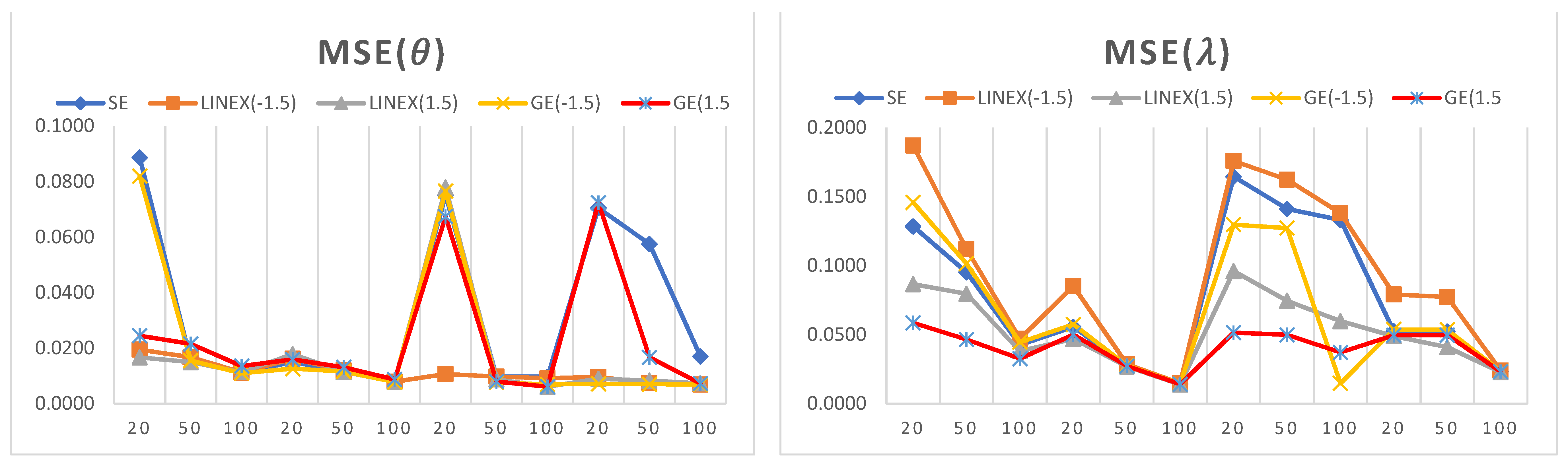
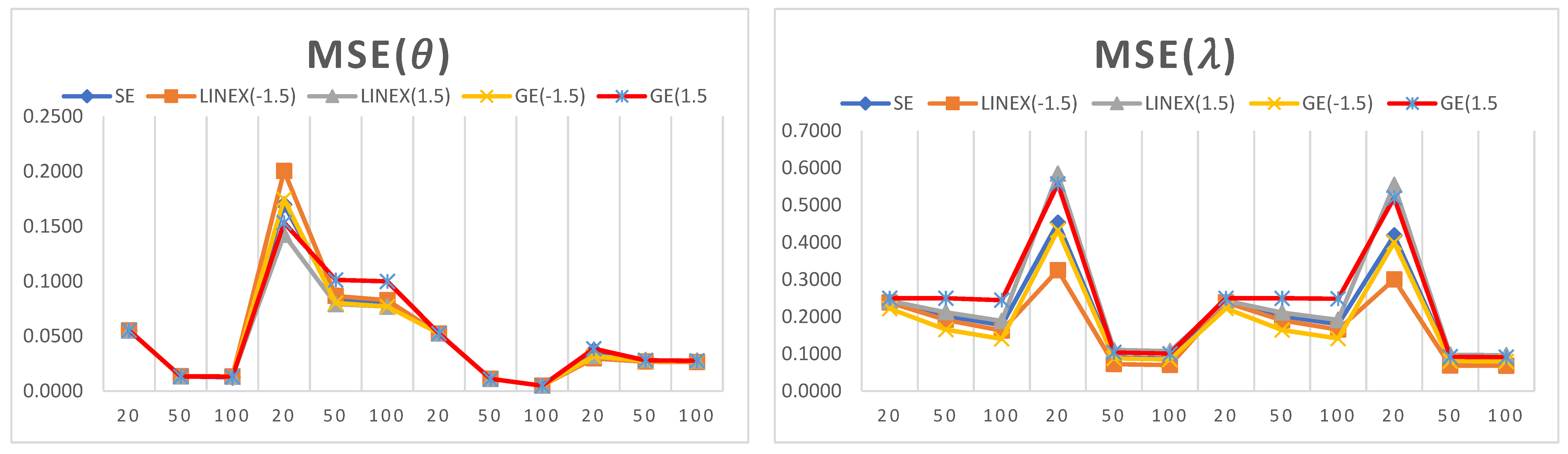
- It can be observed that the estimated values of the model parameters converge to their true values when increasing the sample size. This can be observed since the MSE and biases decrease as the sample size increases, which shows that the proposed estimators are consistent in nature.
- For a small sample size, the LINEX loss function provides the lowest values of MSE and bias when estimating , while the GE loss function provides the lowest values of MSE and bias when estimating .
- For a large sample size, the LINEX loss function provides the lowest values of MSE and bias when estimating both parameters and .
- In almost all cases, the LINEX and GE loss functions produce minimum bias and MSE values, and this is true for different sample sizes. Hence, LINEX and GE are recommended over SE in this study.
- For the credible CI, it is noted that the shortest interval length is obtained when using the LINEX loss function.
- The SE loss function has some advantages over other loss functions under some conditions; for example, when = = 3 and for a small sample size (n = 20), the bias and MSE attain their minimum values when estimating .
- For a fixed value of , the bias decreases when the shape parameter increases. Similarly, for a fixed value of , the bias decreases when increases.
- The length of the credible interval decreases when the sample size increases, and this is true for all loss functions under study.
- For almost all small-size cases, the first discrete analogue DGPD1 has the least bias and lowest MSE for different parameter values.
- For a large sample size, it is observed that the MSE attains its minimum values when using the second analogue, DGPD2.
- The advantage of using the third analogue, DGPD3, appears when finding the credible interval for the parameter using the GE loss function, where the interval length reaches its minimum value.
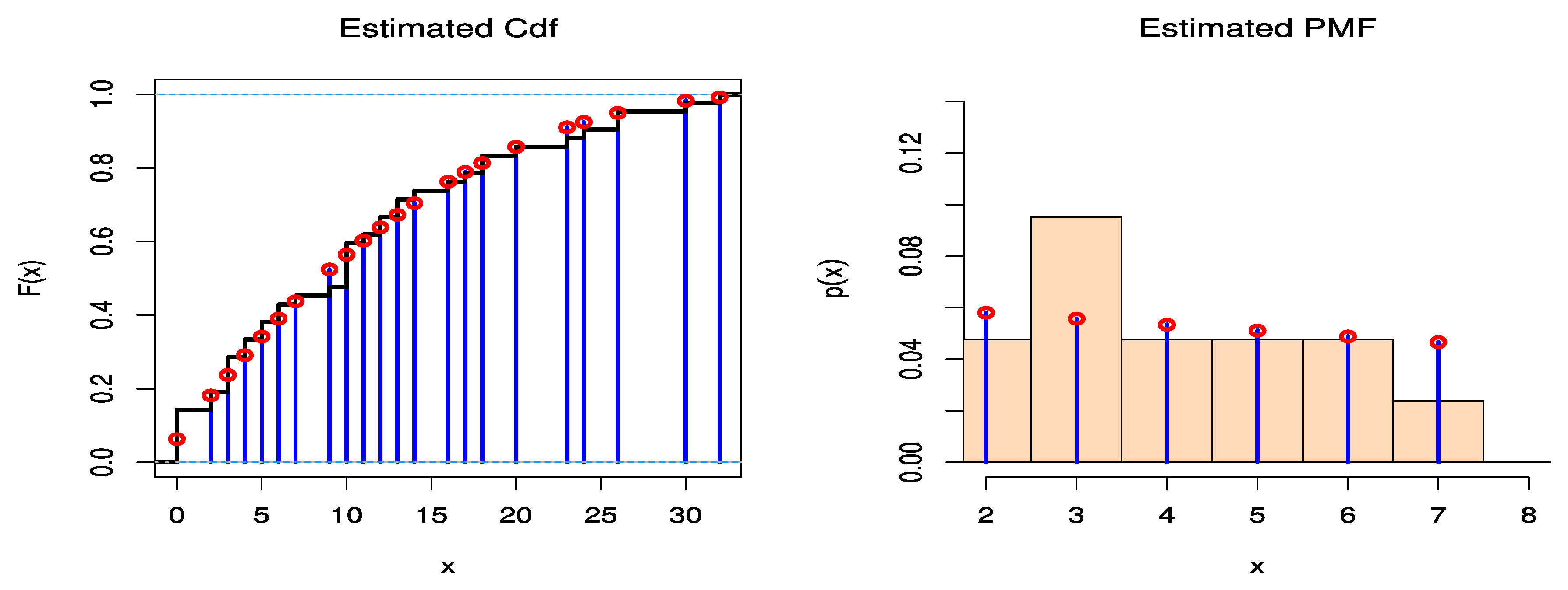
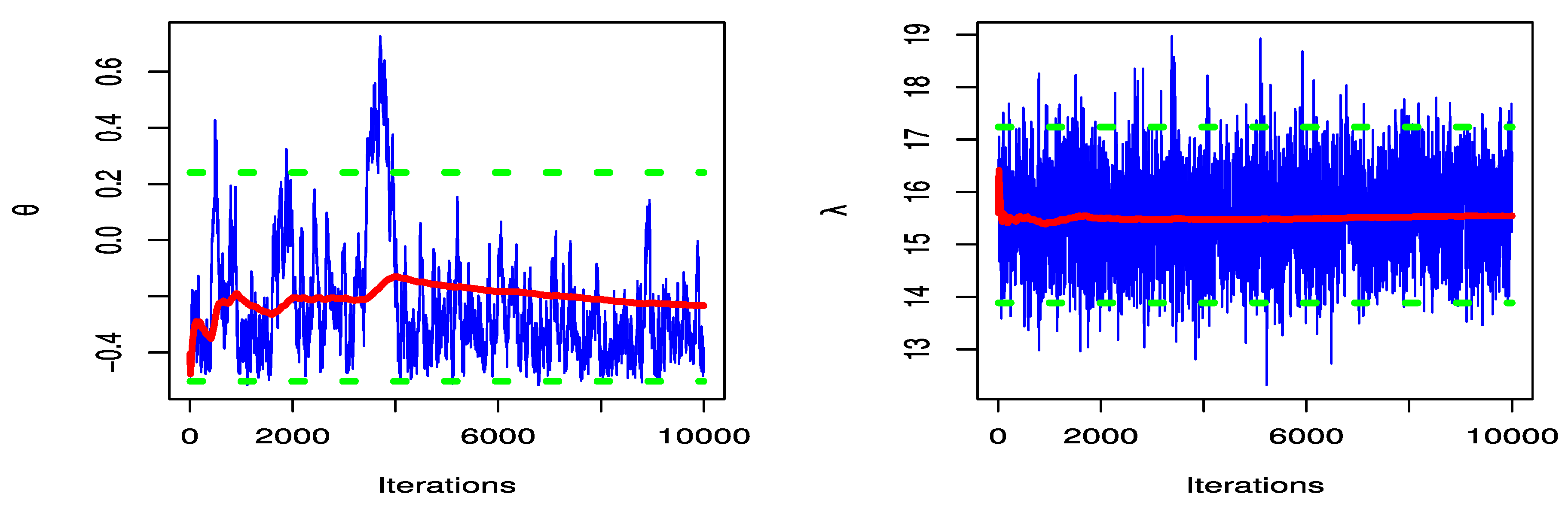
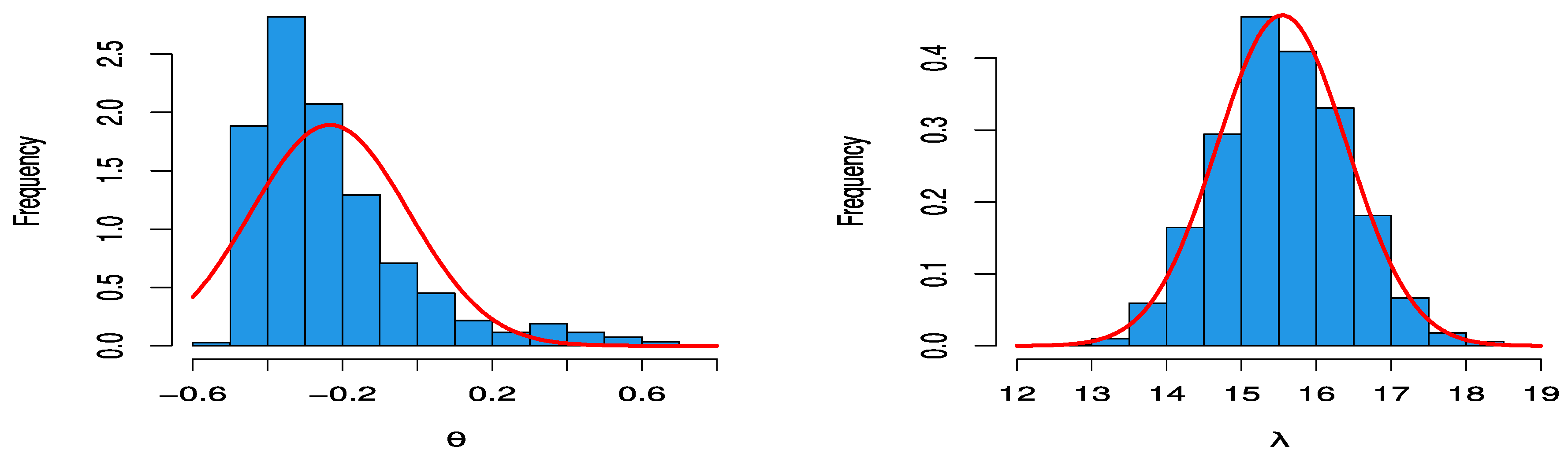
5. Real Data Examples
6. Conclusions
Author Contributions
Funding
Institutional Review Board Statement
Informed Consent Statement
Data Availability Statement
Conflicts of Interest
References
- Xekalaki, E. Hazard function and life distributions in discrete time. Commun. Stat. Theory Methods 1983, 12, 2503–2509. [Google Scholar] [CrossRef]
- Hitha, N.; Nair, N.U. Characterization of some discrete models by properties of residual life function. Calcutta Stat. Assoc. Bull. 1989, 38, 219–223. [Google Scholar] [CrossRef]
- Roy, D.; Gupta, R.P. Classifications of discrete lives. Microelectron. Reliab. 1992, 32, 459–1473. [Google Scholar] [CrossRef]
- Roy, D.; Gupta, R.P. Stochastic modeling through reliability measures in the discrete case. Stat. Probab. Lett. 1999, 43, 197–206. [Google Scholar] [CrossRef]
- Roy, D. On classifications of multivariate life distributions in the discrete set-up. Microelectron. Reliab. 1997, 37, 361–366. [Google Scholar] [CrossRef]
- Roy, D. The discrete normal distribution. Commun. Stat. Theory Methods 2003, 32, 1871–1883. [Google Scholar] [CrossRef]
- Roy, D. Discrete Rayleigh distribution. IEEE. Trans. Reliab. 2004, 53, 255–260. [Google Scholar] [CrossRef]
- Roy, D.; Ghosh, T. A New Discretization Approach with Application in Reliability Estimation. IEEE Trans. Reliab. 2009, 58, 456–461. [Google Scholar] [CrossRef]
- Bracquemond, C.; Gaudoin, O. A survey on discrete life time distributions. Int. J. Reliab. Qual. Saf. Eng. 2003, 10, 69–98. [Google Scholar] [CrossRef]
- Lai, C.D. Issues concerning constructions of discrete lifetime models. Qual. Technol. Quant. Manag. 2013, 10, 251–262. [Google Scholar] [CrossRef]
- Chakraborty, S. Generating discrete analogues of continuous probability distributions—A survey of methods and constructions. J. Stat. Distrib. Appl. 2015, 2, 6. [Google Scholar] [CrossRef]
- Liu, H.; Hussain, F.; Tan, C.L.; Dash, M. Discretization: An Enabling Technique. Data Min. Knowl. Discov. 2002, 6, 393–423. [Google Scholar] [CrossRef]
- Arnastauskaitė, J.; Ruzgas, T.; Bražėnas, M. An Exhaustive Power Comparison of Normality Tests. Mathematics 2021, 9, 788. [Google Scholar] [CrossRef]
- Korkmaz, S.; Goksuluk, D.; Zararsiz, G. MVN: An R Package for Assessing Multivariate Normality. R J. 2014, 6, 151–162. [Google Scholar] [CrossRef]
- Al-Huniti, A.A.; AL-Dayian, G.R. Discrete Burr type III distribution. Am. J. Math. Stat. 2012, 2, 145–152. [Google Scholar] [CrossRef]
- Bebbington, M.; Lai, C.D.; Wellington, M.; Zitikis, R. The discrete additive Weibull distribution: A bathtub-shaped hazard for discontinuous failure data. Reliab. Eng. Syst. Saf. 2012, 106, 37–44. [Google Scholar] [CrossRef]
- Sarhan, A.M. A two-parameter discrete distribution with a bathtub hazard shape. Commun. Stat. Appl. Methods 2017, 24, 15–27. [Google Scholar] [CrossRef][Green Version]
- Yari, G.; Tondpour, Z. Discrete Burr XII-Gamma Distributions: Properties and Parameter Estimations. Iran. J. Sci. Technol. Trans. A Sci. 2018, 42, 2237–2249. [Google Scholar] [CrossRef]
- Almetwally, E.M.; Ibrahim, G.M. Discrete Alpha Power Inverse Lomax Distribution with Application of COVID-19 Data. Int. J. Appl. Math. 2020, 9, 11–22. [Google Scholar]
- Eliwa, M.S.; Altun, E.; El-Dawoody, M.; El-Morshedy, M. A new three-parameter discrete distribution with associated INAR (1) process and applications. IEEE Access 2020, 8, 91150–91162. [Google Scholar] [CrossRef]
- Almetwally, E.M.; Almongy, H.M.; Saleh, H.A. Managing risk of spreading “COVID-19” in Egypt: Modelling using a discrete Marshall-Olkin generalized exponential distribution. Int. J. Probab. Stat. 2020, 9, 33–41. [Google Scholar]
- Al-Babtain, A.A.; Ahmed, A.H.N.; Afify, A.Z. A New Discrete Analog of the Continuous Lindley Distribution, with Reliability Applications. Entropy 2020, 22, 603. [Google Scholar] [CrossRef] [PubMed]
- Eldeeb, A.S.; Ahsan-Ul-Haq, M.; Babar, A. A Discrete Analog of Inverted Topp-Leone Distribution: Properties, Estimation and Applications. Int. J. Anal. Appl. 2021, 19, 695–708. [Google Scholar]
- Elbatal, I.; Alotaibi, N.; Almetwally, E.M.; Alyami, S.A.; Elgarhy, M. On Odd Perks-G Class of Distributions: Properties, Regression Model, Discretization, Bayesian and Non-Bayesian Estimation, and Applications. Symmetry 2022, 14, 883. [Google Scholar] [CrossRef]
- Nagy, M.; Almetwally, E.M.; Gemeay, A.M.; Mohammed, H.S.; Jawa, T.M.; Sayed-Ahmed, N.; Muse, A.H. The new novel discrete distribution with application on covid-19 mortality numbers in Kingdom of Saudi Arabia and Latvia. Complexity 2021, 2021, 7192833. [Google Scholar] [CrossRef]
- Gillariose, J.; Balogun, O.S.; Almetwally, E.M.; Sherwani, R.A.K.; Jamal, F.; Joseph, J. On the Discrete Weibull Marshall–Olkin Family of Distributions: Properties, Characterizations, and Applications. Axioms 2021, 10, 287. [Google Scholar] [CrossRef]
- Martín, J.; Parra, M.I.; Pizarro, M.M.; Sanjuán, E.L. Baseline Methods for the Parameter Estimation of the Generalized Pareto Distribution. Entropy 2022, 24, 178. [Google Scholar] [CrossRef]
- Huang, C.; Zhao, X.; Cheng, W.; Ji, Q.; Duan, Q.; Han, Y. Statistical Inference of Dynamic Conditional Generalized Pareto Distribution with Weather and Air Quality Factors. Mathematics 2022, 10, 1433. [Google Scholar] [CrossRef]
- Shui, P.-L.; Zou, P.-J.; Feng, T. Outlier-robust truncated maximum likelihood parameter estimators of generalized Pareto distributions. Digit. Signal Process. 2022, 127, 103527. [Google Scholar] [CrossRef]
- He, Y.; Peng, L.; Zhang, D.; Zhao, Z. Risk Analysis via Generalized Pareto Distributions. J. Bus. Econ. Stat. 2021, 40, 852–867. [Google Scholar] [CrossRef]
- Arnold, B.C.; Press, S.J. Compatible Conditional Distributions. J. Am. Stat. Assoc. 1989, 84, 152. [Google Scholar] [CrossRef]
- Karandikar, R.L. On the Markov Chain Monte Carlo (MCMC) method. Sadhana 2006, 31, 81–104. [Google Scholar] [CrossRef]
- Wang, Y.; Zhang, J.; Cai, C.; Lu, W.; Tang, Y. Semiparametric estimation for proportional hazards mixture cure model allowing non-curable competing risk. J. Stat. Plan. Inference 2020, 211, 171–189. [Google Scholar] [CrossRef]
- Xu, A.; Zhou, S.; Tang, Y. A unified model for system reliability evaluation under dynamic operating conditions. IEEE Trans. Reliab. 2021, 70, 65–72. [Google Scholar] [CrossRef]
- Luo, C.; Shen, L.; Xu, A. Modelling and estimation of system reliability under dynamic operating environments and lifetime ordering constraints. Reliab. Eng. Syst. Saf. 2022, 218, 108136. [Google Scholar] [CrossRef]
- Worldometers. Available online: https://www.worldometers.info/coronavirus. (accessed on 1 June 2021).
- Almetwally, E.M.; Abdo, D.A.; Hafez, E.H.; Jawa, T.M.; Sayed-Ahmed, N.; Almongy, H.M. The new discrete distribution with application to COVID-19 Data. Results Phys. 2021, 32, 104987. [Google Scholar] [CrossRef]
- Krishna, H.; Pundir, P.S. Discrete Burr and discrete Pareto distributions. Stat. Methodol. 2009, 6, 177–188. [Google Scholar] [CrossRef]
- Khan, M.A.; Khalique, A.; Abouammoh, A.M. On estimating parameters in a discrete Weibull distribution. IEEE Trans. Reliab. 1989, 38, 348–350. [Google Scholar] [CrossRef]
- Jazi, M.A.; Lai, C.-D.; Alamatsaz, M.H. A discrete inverse Weibull distribution and estimation of its parameters. Stat. Methodol. 2010, 7, 121–132. [Google Scholar] [CrossRef]
- Fisher, P. Negative Binomial Distribution. Ann. Eugen. 1941, 11, 182–787. [Google Scholar] [CrossRef]
- Nekoukhou, V.; Alamatsaz, M.H.; Bidram, H. Discrete generalized exponential distribution of a second type. Statistics 2013, 47, 876–887. [Google Scholar] [CrossRef]
- Gómez-Déniz, E.; Calderín-Ojeda, E. The discrete Lindley distribution: Properties and applications. J. Stat. Comput. Simul. 2011, 81, 1405–1416. [Google Scholar] [CrossRef]


| SE | LINEX (−1.5) | LINEX (1.5) | GE (−1.5) | GE (1.5) | ||||||||||||||
|---|---|---|---|---|---|---|---|---|---|---|---|---|---|---|---|---|---|---|
| n | Bias | MSE | L.CCI | Bias | MSE | L.CCI | Bias | MSE | L.CCI | Bias | MSE | L.CCI | Bias | MSE | L.CCI | |||
| 0.5 | 0.5 | 20 | 0.0247 | 0.0887 | 0.5335 | 0.0601 | 0.0194 | 0.4371 | −0.0066 | 0.0167 | 0.4630 | 0.0450 | 0.0820 | 0.6443 | −0.0870 | 0.0245 | 0.4930 | |
| 0.2946 | 0.1284 | 0.7412 | 0.3597 | 0.1870 | 0.8541 | 0.2368 | 0.0866 | 0.6692 | 0.3190 | 0.1458 | 0.7567 | 0.1631 | 0.0586 | 0.6918 | ||||
| 50 | −0.0130 | 0.0155 | 0.4394 | 0.0034 | 0.0167 | 0.4526 | −0.0289 | 0.0150 | 0.4294 | −0.0020 | 0.0155 | 0.4396 | −0.0750 | 0.0215 | 0.4590 | |||
| 0.2666 | 0.0952 | 0.6031 | 0.2901 | 0.1120 | 0.6405 | 0.2429 | 0.0796 | 0.5616 | 0.2764 | 0.1014 | 0.6067 | 0.2132 | 0.0465 | 0.5528 | ||||
| 100 | −0.0084 | 0.0112 | 0.4062 | −0.0025 | 0.0112 | 0.4070 | −0.0144 | 0.0113 | 0.4062 | −0.0041 | 0.0110 | 0.4023 | −0.0316 | 0.0136 | 0.4360 | |||
| 0.1827 | 0.0424 | 0.3745 | 0.1923 | 0.0470 | 0.3914 | 0.1729 | 0.0381 | 0.3569 | 0.1872 | 0.0444 | 0.3781 | 0.1586 | 0.0326 | 0.3407 | ||||
| 3 | 20 | 0.0353 | 0.0150 | 0.4610 | 0.0680 | 0.0162 | 0.4588 | 0.0064 | 0.0178 | 0.4533 | 0.0537 | 0.0126 | 0.4755 | −0.0642 | 0.0159 | 0.4910 | ||
| 0.0704 | 0.0555 | 0.8743 | 0.1615 | 0.0852 | 0.9396 | −0.0176 | 0.0469 | 0.8464 | 0.0803 | 0.0574 | 0.8773 | 0.0206 | 0.0500 | 0.8675 | ||||
| 50 | 0.0009 | 0.0116 | 0.4267 | 0.0080 | 0.0120 | 0.4324 | −0.0062 | 0.0114 | 0.4220 | 0.0057 | 0.0116 | 0.4274 | −0.0248 | 0.0131 | 0.4528 | |||
| 0.0192 | 0.0276 | 0.6226 | 0.0301 | 0.0287 | 0.6274 | 0.0084 | 0.0269 | 0.6189 | 0.0204 | 0.0277 | 0.6217 | 0.0132 | 0.0274 | 0.6259 | ||||
| 100 | −0.0080 | 0.0079 | 0.3509 | −0.0042 | 0.0079 | 0.3511 | −0.0117 | 0.0079 | 0.3508 | −0.0054 | 0.0078 | 0.3480 | −0.0214 | 0.0087 | 0.3554 | |||
| 0.0230 | 0.0143 | 0.4554 | 0.0285 | 0.0148 | 0.4601 | 0.0175 | 0.0139 | 0.4513 | 0.0236 | 0.0143 | 0.4552 | 0.0200 | 0.0141 | 0.4526 | ||||
| 3 | 0.5 | 20 | 0.0121 | 0.0751 | 0.3389 | 0.0512 | 0.0107 | 0.3506 | −0.0595 | 0.0779 | 0.3306 | 0.0164 | 0.0766 | 0.3387 | −0.0935 | 0.0674 | 0.3351 | |
| 0.2173 | 0.1645 | 0.8449 | 0.4302 | 0.1759 | 1.0064 | 0.2412 | 0.0961 | 0.7222 | 0.2527 | 0.1297 | 0.8780 | 0.2331 | 0.0514 | 0.7289 | ||||
| 50 | −0.0037 | 0.0098 | 0.3079 | 0.0348 | 0.0098 | 0.3335 | −0.0405 | 0.0087 | 0.2944 | 0.0005 | 0.0076 | 0.3612 | −0.0245 | 0.0080 | 0.2998 | |||
| 0.2719 | 0.1411 | 0.5948 | 0.3410 | 0.1623 | 0.6569 | 0.2115 | 0.0745 | 0.5119 | 0.2499 | 0.1272 | 0.6932 | 0.1251 | 0.0499 | 0.5576 | ||||
| 100 | −0.0321 | 0.0097 | 0.3052 | 0.0018 | 0.0092 | 0.3060 | −0.0655 | 0.0061 | 0.2343 | −0.0284 | 0.0069 | 0.3509 | −0.0151 | 0.0061 | 0.2534 | |||
| 0.1317 | 0.1330 | 0.5668 | 0.3723 | 0.1380 | 0.6074 | 0.2068 | 0.0598 | 0.5096 | 0.2338 | 0.0148 | 0.6809 | 0.1021 | 0.0371 | 0.4620 | ||||
| 3 | 20 | 0.0039 | 0.0705 | 0.3629 | 0.0430 | 0.0096 | 0.4776 | −0.0339 | 0.0090 | 0.3625 | 0.0082 | 0.0071 | 0.3986 | −0.0175 | 0.0724 | 0.4327 | ||
| 0.0440 | 0.0524 | 0.8789 | 0.1402 | 0.0791 | 0.9525 | −0.0487 | 0.0489 | 0.8914 | 0.0545 | 0.0538 | 0.8868 | −0.0091 | 0.0496 | 0.8982 | ||||
| 50 | 0.0038 | 0.0575 | 0.3339 | 0.0421 | 0.0075 | 0.3526 | −0.0333 | 0.0083 | 0.3348 | 0.0080 | 0.0070 | 0.3368 | −0.0172 | 0.0167 | 0.3383 | |||
| 0.0443 | 0.0522 | 0.8095 | 0.1370 | 0.0773 | 0.8957 | −0.0451 | 0.0409 | 0.8679 | 0.0544 | 0.0535 | 0.7960 | −0.0069 | 0.0497 | 0.8517 | ||||
| 100 | −0.0152 | 0.0170 | 0.3049 | −0.0080 | 0.0069 | 0.3489 | −0.0224 | 0.0073 | 0.4917 | −0.0144 | 0.0069 | 0.3049 | −0.0192 | 0.0072 | 0.2491 | |||
| 0.0112 | 0.0233 | 0.5707 | 0.0197 | 0.0240 | 0.5772 | 0.0028 | 0.0228 | 0.5787 | 0.0122 | 0.0234 | 0.5702 | 0.0065 | 0.0231 | 0.5744 | ||||
| SE | LINEX (−1.5) | LINEX (1.5) | GE (−1.5) | GE (1.5) | ||||||||||||||
|---|---|---|---|---|---|---|---|---|---|---|---|---|---|---|---|---|---|---|
| n | Bias | MSE | L.CCI | Bias | MSE | L.CCI | Bias | MSE | L.CCI | Bias | MSE | L.CCI | Bias | MSE | L.CCI | |||
| 0.5 | 0.5 | 20 | −0.1145 | 0.0668 | 0.7749 | −0.1110 | 0.0652 | 0.7740 | −0.1177 | 0.0681 | 0.7734 | −0.1086 | 0.0630 | 0.7578 | −0.1349 | 0.0793 | 0.7870 | |
| −0.4889 | 0.2491 | 0.0185 | −0.4856 | 0.2459 | 0.0247 | −0.4911 | 0.2412 | 0.0142 | −0.4684 | 0.2296 | 0.0421 | −0.4993 | 0.2493 | 0.0039 | ||||
| 50 | −0.0972 | 0.0525 | 0.7273 | −0.0951 | 0.0518 | 0.7252 | −0.0991 | 0.0531 | 0.7284 | −0.0945 | 0.0511 | 0.7180 | −0.1075 | 0.0574 | 0.7516 | |||
| −0.4901 | 0.2402 | 0.0177 | −0.4878 | 0.2380 | 0.0204 | −0.4916 | 0.2417 | 0.0157 | −0.4732 | 0.2240 | 0.0291 | −0.4980 | 0.2480 | 0.0092 | ||||
| 100 | −0.0522 | 0.0186 | 0.4950 | −0.0515 | 0.0184 | 0.4941 | −0.0529 | 0.0187 | 0.4963 | −0.0516 | 0.0184 | 0.4927 | −0.0550 | 0.0192 | 0.4994 | |||
| −0.4747 | 0.2254 | 0.0255 | −0.4696 | 0.2206 | 0.0293 | −0.4782 | 0.2288 | 0.0243 | −0.4505 | 0.2031 | 0.0335 | −0.4919 | 0.2420 | 0.0193 | ||||
| 3 | 20 | 0.1424 | 0.0378 | 0.4501 | 0.1906 | 0.0604 | 0.5041 | 0.1000 | 0.0234 | 0.4023 | 0.1647 | 0.0459 | 0.4579 | 0.0206 | 0.0143 | 0.4190 | ||
| −0.0366 | 0.0591 | 0.8932 | 0.0534 | 0.0699 | 0.9843 | −0.1246 | 0.0681 | 0.8693 | −0.0265 | 0.0588 | 0.9016 | −0.0881 | 0.0641 | 0.8811 | ||||
| 50 | 0.0248 | 0.0145 | 0.4295 | 0.0328 | 0.0154 | 0.4373 | 0.0167 | 0.0138 | 0.4241 | 0.0300 | 0.0147 | 0.4286 | −0.0031 | 0.0137 | 0.4048 | |||
| −0.0371 | 0.0312 | 0.6886 | −0.0256 | 0.0300 | 0.6766 | −0.0487 | 0.0327 | 0.6941 | −0.0358 | 0.0310 | 0.6877 | −0.0437 | 0.0323 | 0.6971 | ||||
| 100 | 0.0068 | 0.0077 | 0.3405 | 0.0104 | 0.0078 | 0.3384 | 0.0032 | 0.0075 | 0.3367 | 0.0092 | 0.0077 | 0.3346 | −0.0056 | 0.0079 | 0.3475 | |||
| −0.0257 | 0.0113 | 0.4118 | −0.0213 | 0.0109 | 0.4001 | −0.0302 | 0.0117 | 0.4212 | −0.0252 | 0.0113 | 0.4104 | −0.0283 | 0.0116 | 0.4019 | ||||
| 3 | 0.5 | 20 | 0.0315 | 0.0547 | 0.9001 | 0.0348 | 0.0549 | 0.9038 | 0.0282 | 0.0543 | 0.8926 | 0.0318 | 0.0547 | 0.9004 | 0.0297 | 0.0546 | 0.8976 | |
| −0.4798 | 0.2309 | 0.0569 | −0.4715 | 0.2240 | 0.0845 | −0.4850 | 0.2355 | 0.0409 | −0.4503 | 0.2046 | 0.1119 | −0.4998 | 0.2498 | 0.0006 | ||||
| 50 | 0.0211 | 0.0169 | 0.4877 | 0.0234 | 0.0171 | 0.4883 | 0.0187 | 0.0166 | 0.4842 | 0.0214 | 0.0169 | 0.4879 | 0.0198 | 0.0168 | 0.4854 | |||
| −0.3902 | 0.1568 | 0.2287 | −0.3676 | 0.1406 | 0.2581 | −0.4090 | 0.1710 | 0.1935 | −0.3388 | 0.1195 | 0.2469 | −0.4981 | 0.2490 | 0.0003 | ||||
| 100 | 0.0183 | 0.0085 | 0.3602 | 0.0199 | 0.0086 | 0.3628 | 0.0166 | 0.0083 | 0.3570 | 0.0184 | 0.0085 | 0.3605 | 0.0173 | 0.0084 | 0.3587 | |||
| −0.3494 | 0.1252 | 0.1901 | −0.3246 | 0.1087 | 0.2058 | −0.3715 | 0.1407 | 0.1709 | −0.3002 | 0.0929 | 0.1893 | −0.4992 | 0.2049 | 0.0002 | ||||
| 3 | 20 | 0.0932 | 0.0255 | 0.6319 | 0.1333 | 0.0251 | 0.3280 | 0.0544 | 0.0195 | 0.5306 | 0.0975 | 0.0263 | 0.5319 | 0.0719 | 0.0219 | 0.5632 | ||
| 0.0225 | 0.0618 | 0.9381 | 0.1175 | 0.0857 | 1.0463 | −0.0703 | 0.0608 | 0.8915 | 0.0330 | 0.0629 | 0.9506 | −0.0309 | 0.0606 | 0.8925 | ||||
| 50 | 0.0546 | 0.0203 | 0.5208 | 0.0640 | 0.0219 | 0.5218 | 0.0453 | 0.0189 | 0.5090 | 0.0556 | 0.0204 | 0.5209 | 0.0495 | 0.0196 | 0.5177 | |||
| −0.0173 | 0.0281 | 0.6513 | −0.0059 | 0.0272 | 0.6505 | −0.0287 | 0.0293 | 0.6510 | −0.0160 | 0.0279 | 0.6504 | −0.0238 | 0.0290 | 0.6459 | ||||
| 100 | 0.0451 | 0.0115 | 0.3816 | 0.0495 | 0.0123 | 0.3872 | 0.0406 | 0.0107 | 0.3728 | 0.0455 | 0.0116 | 0.3835 | 0.0426 | 0.0111 | 0.3791 | |||
| −0.0042 | 0.0115 | 0.4137 | 0.0000 | 0.0115 | 0.4164 | −0.0083 | 0.0117 | 0.4146 | −0.0037 | 0.0115 | 0.4138 | −0.0065 | 0.0116 | 0.4162 | ||||
| SE | LINEX (−1.5) | LINEX (1.5) | GE (−1.5) | GE (1.5) | ||||||||||||||
|---|---|---|---|---|---|---|---|---|---|---|---|---|---|---|---|---|---|---|
| n | Bias | MSE | L.CCI | Bias | MSE | L.CCI | Bias | MSE | L.CCI | Bias | MSE | L.CCI | Bias | MSE | L.CCI | |||
| 0.5 | 0.5 | 20 | 0.0231 | 0.0552 | 0.9405 | 0.0248 | 0.0552 | 0.9396 | 0.0214 | 0.0550 | 0.9399 | 0.0236 | 0.0552 | 0.9397 | 0.0208 | 0.0552 | 0.9422 | |
| −0.4908 | 0.2409 | 0.0134 | −0.4879 | 0.2381 | 0.0189 | −0.4927 | 0.2428 | 0.0097 | −0.4710 | 0.2219 | 0.0349 | −0.4998 | 0.2498 | 0.0005 | ||||
| 50 | 0.0067 | 0.0134 | 0.4749 | 0.0075 | 0.0135 | 0.4757 | 0.0058 | 0.0133 | 0.4719 | 0.0069 | 0.0134 | 0.4750 | 0.0055 | 0.0133 | 0.4718 | |||
| −0.4505 | 0.2032 | 0.0495 | −0.4374 | 0.1916 | 0.0645 | −0.4603 | 0.2120 | 0.0397 | −0.4064 | 0.1655 | 0.0713 | −0.4999 | 0.2499 | 0.0002 | ||||
| 100 | 0.0291 | 0.0124 | 0.4307 | 0.0303 | 0.0134 | 0.4333 | 0.0028 | 0.0131 | 0.4255 | 0.0295 | 0.0130 | 0.4312 | 0.0274 | 0.0131 | 0.4246 | |||
| −0.4204 | 0.1771 | 0.0642 | −0.4030 | 0.1628 | 0.0796 | −0.4342 | 0.1887 | 0.0521 | −0.3742 | 0.1405 | 0.0841 | −0.4946 | 0.2446 | 0.0097 | ||||
| 3 | 20 | 0.0783 | 0.1698 | 1.3450 | 0.1181 | 0.2003 | 1.3980 | 0.0418 | 0.1425 | 1.2318 | 0.0989 | 0.1747 | 1.3478 | −0.0302 | 0.1534 | 1.2360 | ||
| −0.5967 | 0.4528 | 1.0853 | −0.4890 | 0.3254 | 0.9966 | −0.6941 | 0.5849 | 1.1111 | −0.5818 | 0.4329 | 1.0580 | −0.6704 | 0.5575 | 1.1327 | ||||
| 50 | −0.0389 | 0.0829 | 0.9246 | −0.0219 | 0.0866 | 0.9413 | −0.0558 | 0.0793 | 0.8868 | −0.0247 | 0.0803 | 0.9205 | −0.1120 | 0.1012 | 0.9059 | |||
| −0.2242 | 0.0906 | 0.7755 | −0.1974 | 0.0726 | 0.6992 | −0.2507 | 0.1108 | 0.8376 | −0.2207 | 0.0881 | 0.7653 | −0.2414 | 0.1040 | 0.8219 | ||||
| 100 | −0.0457 | 0.0799 | 0.8656 | −0.0290 | 0.0828 | 0.9041 | −0.0622 | 0.0770 | 0.8300 | −0.0314 | 0.0769 | 0.8707 | −0.1192 | 0.0999 | 0.8511 | |||
| −0.2203 | 0.0876 | 0.7755 | −0.1938 | 0.0700 | 0.6992 | −0.2466 | 0.1073 | 0.8376 | −0.2169 | 0.0851 | 0.7653 | −0.2373 | 0.1007 | 0.8219 | ||||
| 3 | 0.5 | 20 | −0.0119 | 0.0524 | 0.8664 | −0.0101 | 0.0523 | 0.8657 | −0.0137 | 0.0524 | 0.8661 | −0.0117 | 0.0524 | 0.8664 | −0.0129 | 0.0525 | 0.8665 | |
| −0.4911 | 0.2411 | 0.0129 | −0.4884 | 0.2385 | 0.0180 | −0.4929 | 0.2429 | 0.0099 | −0.4717 | 0.2226 | 0.0330 | −0.4998 | 0.2498 | 0.0005 | ||||
| 50 | 0.0029 | 0.0112 | 0.4081 | 0.0036 | 0.0112 | 0.4077 | 0.0022 | 0.0111 | 0.4081 | 0.0030 | 0.0112 | 0.4080 | 0.0025 | 0.0112 | 0.4082 | |||
| −0.4495 | 0.2023 | 0.0525 | −0.4360 | 0.1905 | 0.0672 | −0.4596 | 0.2113 | 0.0404 | −0.4048 | 0.1643 | 0.0736 | −0.4999 | 0.2499 | 0.0002 | ||||
| 100 | 0.0034 | 0.0049 | 0.2857 | 0.0040 | 0.0049 | 0.2853 | 0.0029 | 0.0049 | 0.2860 | 0.0035 | 0.0049 | 0.2857 | 0.0031 | 0.0049 | 0.2859 | |||
| −0.4238 | 0.1799 | 0.0538 | −0.4064 | 0.1654 | 0.0653 | −0.4375 | 0.1916 | 0.0439 | −0.3757 | 0.1415 | 0.0652 | −0.4986 | 0.2486 | 0.0026 | ||||
| 3 | 20 | −0.0261 | 0.0370 | 0.6937 | 0.0126 | 0.0297 | 0.6419 | −0.0640 | 0.0320 | 0.6453 | −0.0218 | 0.0317 | 0.5972 | −0.0478 | 0.0386 | 0.6255 | ||
| −0.6123 | 0.4187 | 0.7591 | −0.5002 | 0.3003 | 0.8630 | −0.7168 | 0.5547 | 0.7219 | −0.5969 | 0.4002 | 0.7670 | −0.6900 | 0.5200 | 0.7443 | ||||
| 50 | −0.0277 | 0.0274 | 0.5896 | −0.0182 | 0.0268 | 0.5730 | −0.0372 | 0.0282 | 0.6052 | −0.0267 | 0.0273 | 0.5874 | −0.0331 | 0.0280 | 0.6017 | |||
| −0.2226 | 0.0826 | 0.7089 | −0.2005 | 0.0687 | 0.6596 | −0.2449 | 0.0978 | 0.7456 | −0.2198 | 0.0807 | 0.7030 | −0.2368 | 0.0925 | 0.7363 | ||||
| 100 | −0.0252 | 0.0270 | 0.5209 | −0.0159 | 0.0264 | 0.5730 | −0.0345 | 0.0277 | 0.6052 | −0.0242 | 0.0269 | 0.5874 | −0.0305 | 0.0276 | 0.6017 | |||
| −0.2207 | 0.0816 | 0.6709 | −0.1990 | 0.0680 | 0.6596 | −0.2423 | 0.0965 | 0.7456 | −0.2179 | 0.0798 | 0.7030 | −0.2344 | 0.0913 | 0.7363 | ||||
| Estimates | KS-Test | Chi2-Test | AIC | CAIC | BIC | HQIC | ||
|---|---|---|---|---|---|---|---|---|
| DGP | −0.4052 | 0.1429 | 35.2645 | 284.7945 | 285.1021 | 288.2698 | 286.0683 | |
| 15.6070 | 0.3581 | 0.3164 | ||||||
| DMOITL | 16.5627 | 0.1429 | 49.3821 | 297.3120 | 297.6197 | 300.7873 | 298.5859 | |
| 1.8434 | 0.3581 | 0.0255 | ||||||
| DB | 1.6460 | 0.3209 | 94.9821 | 325.9139 | 326.2216 | 329.3892 | 327.1877 | |
| 0.7401 | 0.0004 | 0.0000 | ||||||
| DW | 0.9297 | 0.1429 | 38.7117 | 288.3261 | 288.6338 | 291.8014 | 289.6000 | |
| 1.0837 | 0.3581 | 0.1925 | ||||||
| DIW | 0.0642 | 0.2034 | 64.6983 | 315.3363 | 315.6439 | 318.8116 | 316.6101 | |
| 0.7797 | 0.0618 | 0.0005 | ||||||
| NB | P | 0.8015 | 0.3072 | 28307.5450 | 431.9343 | 432.0343 | 433.6720 | 432.5712 |
| 0.0007 | 0.0000 | |||||||
| Poisson | 10.4048 | 0.3277 | 677700.3282 | 482.2590 | 482.3590 | 483.9967 | 482.8960 | |
| 0.0002 | 0.0000 | |||||||
| DGE | 0.9124 | 0.1595 | 38.3097 | 288.6633 | 288.9710 | 292.1386 | 289.9371 | |
| 0.9986 | 0.2359 | 0.2049 | ||||||
| DAPL | 48.5629 | 0.1804 | 44.5099 | 305.8090 | 306.4406 | 311.0221 | 307.7198 | |
| 3.1137 | 0.1301 | 0.0697 | ||||||
| 0.5752 | ||||||||
| DL | 0.8437 | 0.1231 | 51.3964 | 289.7677 | 289.8677 | 291.5054 | 290.4046 | |
| 0.5479 | 0.0163 | |||||||
| MLE | Bayesian | |||
|---|---|---|---|---|
| Estimates | SE | Estimates | SE | |
| −0.4052 | 0.1651 | −0.2337 | 0.1209 | |
| 15.6070 | 3.3902 | 15.5417 | 0.8679 | |
| MLE | Bayesian | |||
|---|---|---|---|---|
| Estimates | SE | Estimates | SE | |
| −0.491911 | 0.103421 | −0.41147 | 0.093889 | |
| 33.312755 | 5.266817 | 33.34727 | 0.886706 | |
Publisher’s Note: MDPI stays neutral with regard to jurisdictional claims in published maps and institutional affiliations. |
© 2022 by the authors. Licensee MDPI, Basel, Switzerland. This article is an open access article distributed under the terms and conditions of the Creative Commons Attribution (CC BY) license (https://creativecommons.org/licenses/by/4.0/).
Share and Cite
Haj Ahmad, H.; Almetwally, E.M. Generating Optimal Discrete Analogue of the Generalized Pareto Distribution under Bayesian Inference with Applications. Symmetry 2022, 14, 1457. https://doi.org/10.3390/sym14071457
Haj Ahmad H, Almetwally EM. Generating Optimal Discrete Analogue of the Generalized Pareto Distribution under Bayesian Inference with Applications. Symmetry. 2022; 14(7):1457. https://doi.org/10.3390/sym14071457
Chicago/Turabian StyleHaj Ahmad, Hanan, and Ehab M. Almetwally. 2022. "Generating Optimal Discrete Analogue of the Generalized Pareto Distribution under Bayesian Inference with Applications" Symmetry 14, no. 7: 1457. https://doi.org/10.3390/sym14071457
APA StyleHaj Ahmad, H., & Almetwally, E. M. (2022). Generating Optimal Discrete Analogue of the Generalized Pareto Distribution under Bayesian Inference with Applications. Symmetry, 14(7), 1457. https://doi.org/10.3390/sym14071457