1. Introduction
The notion of kinetic energy is present even in Galileo’s work, where he encompasses a concept of interconvertibility between the kinetic and potential energy. The study regarding this notion continued along the years, catching the interest of several mathematicians such as Descartes or Leibnitz. The product mv
2 was first referred to as ‘energy’ by Thomas Young in 1807 and in 1853 William Rankine determined a distinction between ‘potential energy’ and ‘actual energy’, which was previously called ‘kinetic energy’ by Kelvin. The notion of kinetic energy, with its modern meaning, started being used widely only after 1870 [
1].
Today, kinetic energy is a fundamental notion in Newtonian dynamics, and its use is found in the theorem of kinetic energy as a general form of mathematical representation, the differential form. By successive transformations, this theorem can degenerate into the other two fundamental theorems, the momentum theorem, and the angular momentum theorem [
2,
3,
4,
5].
The decisive role of kinetic energy is found in analytical dynamics as a central function in Lagrange’s equations of second order, in Hamilton’s equations and in the Hamilton–Ostrogradski variational principle [
6].
For the first time, the phrase “acceleration energy” was highlighted by Paul Appell in 1899 when establishing the dynamics equations of nonholonomic mechanical systems. Through the contribution of J. W. Gibbs to these equations, they received the name Gibbs–Appell equations. In fast-moving mechanical systems, such as serial and parallel robots, rapid movements develop, in which higher-order linear and angular accelerations play an important role. Starting from the Appell function, then called acceleration energy, over time, higher-order acceleration energies developed in analytical dynamics for any material system subjected to rapid motion, especially for bodies in absolute general motion. As a result, higher-order equations of analytical dynamics have been developed to reflect the presence of accelerations specific to fast motions [
3,
7,
8,
9]. Experimentally, the presence of higher-order accelerations was found when the first-order acceleration was
.
This paper aims to establish mathematical relations between kinetic energy and first-order acceleration energy for bodies in general motion and for multibody systems. The first part of the paper is devoted to the expressions of kinetic energy known in the literature [
10,
11,
12,
13], starting from the material point and the system of material points, continuing with König’s theorem specific to general motion and ending with multibody systems, the last one considering the serial structures of robots as an example. Additionally, some expressions of kinetic energy based on higher-order accelerations are presented.
The second part of this paper is devoted to the acceleration energy of first order with expressions for the material point and the system of material points and with new expressions for the body in general motion and multibody systems, highlighting the components consisting in higher-order accelerations.
The third part of this paper is devoted to establishing the relations between the kinetic energy and acceleration energy of first order, as well as their implementation in the equations of dynamics starting from the generalization of the Gibbs–Appell equations. For justifying the validity of the obtained relation, an application is presented. It refers to a 2TR robot structure, which was mathematically modeled for the purpose of being implemented in a technological process involving the hot rolling and the processing of pipes by using any other methods than welding. The expression for kinetic energy using classic formulations in the case of the 2TR robot structure is determined. By applying the relation between the kinetic and acceleration energy presented in the paper, the expression of the acceleration energy is obtained. The robot is implemented in a work process and modelled using the polynomial interpolation functions.
Using MATLAB, the time variation laws for the generalized variable, kinetic energy and acceleration energies of first, second and third order are obtained.
2. Formulations on Kinetic Energy
2.1. Material Point and Discrete System of Material Points
In a real physical process, any change in the dynamic state of a material system represents a mechanical motion whose measurement at a given moment is the kinetic energy considered a dynamic-state quantity. The transfer of the kinetic energy between two physical states of a material system is measured by the mechanical work considering a dynamic process quantity. From the equivalence between the mechanical work and the energy transfer in an infinitely short elementary time interval, it resulted in the current form of kinetic energy for a material point and for a system of material points.
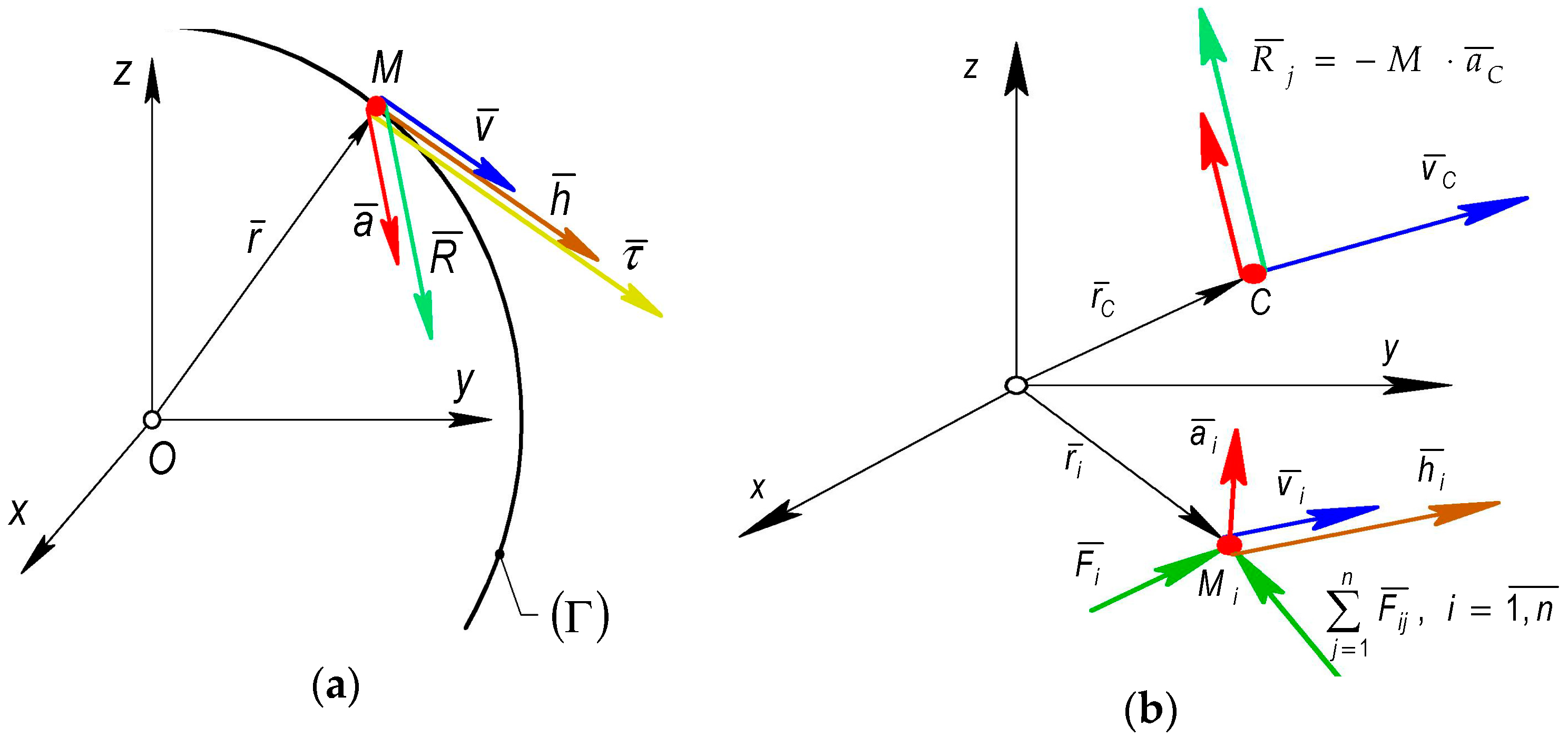
According to
Figure 1, it is considered a point and a system of
n material points subjected to mechanical interactions and to exterior links.
The vector equation that expresses the position of each material point is given by:
where
represent the independent parameters that univocally express the motion of the system.
According to [
11], the following expressions define the velocity and acceleration corresponding to each material particle:
To determine the mathematical relations between the kinetic energy and the acceleration energy, for any mechanical system, we had to know the time derivative of higher order. Therefore, according to [
12], the following identity exists between the partial derivatives of higher orders of the position vectors, the linear velocity and acceleration:
where
m = 1, 2, 3, … are the derivative order.
The kinetic energy for a material particle and its derivatives of first and second order with respect to time are given by:
As a result, the following expressions were obtained:
where
.
In case of a discrete system of material points
, the kinetic energy was:
For the same discrete system of material points, the time derivative of the order (k ≥ 1) of kinetic energy was defined by the expression:
The expressions presented above were further used in the following sections for establishing the mathematical relation between the dynamic quantities and .
2.2. Multibody Systems
For multibody systems (for example, a robot mechanical structure), the generalized coordinates which define the mechanical motion become a function of time. Thus, the time derivatives, as well as the partial derivatives, could be applied.
The column vector of the generalized coordinates
, for a certain configuration different from the initial configuration
, had the following mathematical expression [
3]:
where
are called the generalized coordinates (the degrees of freedom for the mechanical system).
Figure 2 represents the mechanical structure of a serial robot, considered as a multibody system.
The generalized variables of higher order could be developed according to [
12], considering the current and fast mechanical motions as:
where the index
m is the order of the time derivative (
m ≥ 1).
Considering multibody systems, with
kinetic ensembles, the kinematic parameters that expressed the absolute translation motion of each kinetic ensemble were determined as a function of the generalized variables
with the following relations:
They are called the vector equation of the absolute translation motion, of the absolute velocity and acceleration, respectively, of the mass center of each kinetic ensemble from the mechanical system. Like (4), the following differential identities could also be written:
where
are the order of the time derivative.
Additionally, according to [
12], the following relations could be written between the time derivatives of the kinematic parameters:
where
The resultant rotation motion was defined by the angular vector:
where
is the angular transfer matrix which is a function of the orientation angles.
The same angular vector could be expressed using functions of the matrix exponentials as shown in [
3]:
where
and
are the Cartesian axes and
are the unit vectors of the axes around which the rotations were performed with the angles
.
In the papers [
11,
12], the existence of the following identities was proven:
where
represents the angular acceleration vector and for
, the angular velocity in the resultant rotation motion. The operator
, given by:
determines the difference between the kinematic parameters of the resultant translation and the ones of the resultant rotation.
Considering paper [
11], the linear velocity and acceleration of the mass center above shown in (13) and (14) the angular velocity that characterized each ensemble of the mechanical system were established with the expressions:
When dealing with fast motions, the higher-order time derivatives were used.
The significance of the terms contained by these expressions was found in (16) and (21).
Remark: The above differential expressions (15), (16) and (21)–(26) were compulsorily used in the relation between the kinetic energy and acceleration energy.
According to König’s theorem for kinetic energy, the kinetic energy of a multibody mechanical system can be determined using the expression:
and
is the number of kinetic ensembles of the mechanical system.
Considering (23) and (24), the two components of the kinetic energy specific for the resultant translation and resultant rotation, respectively, were written as:
According to [
2,
4], in the expression (30), the symbol
represents the axial-centrifugal inertia tensor, that defines the variation law with respect to concurrent frames in the mass center:
and
. It was expressed with the following matrix formula:
where:
where
is the skew symmetric matrix associated with the position of vector
.
The time derivatives of the higher order of kinetic energy necessary to study its relation to acceleration energy can be written as follows:
where the symbols from (32) have the significance from (9) to (10).
3. The Acceleration Energy of First Order
The present paragraph is devoted to a fundamental study of the existence within the mechanical systems, of some superior forms of energy, corresponding to higher-order accelerations. As a result, the expression that defines the energy of first-order accelerations, also known as Appell’s function, was shown in an explicit form [
4,
8]. Starting from the case of a material point or the system of material points analyzed by Appell within this paragraph, the energy of first-order accelerations for a mechanical system in absolute general motion was determined. The dynamic study was applied to a mechanical system (material point, body and body systems) and acted by a system of active external forces, characterized by a certain law of variation with time. Thus, the system of active forces, which generates a uniformly varied mechanical movement, generally becomes a function of position, velocity and acceleration, and by the time parameter [
14,
15,
16,
17,
18,
19].
Under the action of the active forces, the mechanical system was subjected to fast movements, for which it was proved experimentally that the linear acceleration had the following value: . Thus, within the mechanical system, the so-called higher-order accelerations were developed. From a dynamical point of view, the higher-order accelerations were included in expressions of the acceleration energies.
From a material point, considering (36), the acceleration was defined according to:
As a result, the acceleration energy of first order, in the case of a material point, became:
In the case of a discrete system of material points, according to (4) and (33), the acceleration energy of first order (Appell’s function) was expressed with the relations:
where:
After a few transformations, the following form was obtained:
For the fast motions, the time derivative of the higher order of the acceleration energy of first order was determined by means of the following expression:
The significance of the terms contained in (37) is presented below:
According to [
11], in the case of body systems (i.e., robot structures), the acceleration energy of first order was defined as:
The significance of the terms contained in (41) and (42) was already explained in the previous sections. Considering the fast motions of the mechanical systems, the acceleration energy could be written as a function of higher-order time derivatives of the position vectors of the mass center and of the angular vectors of the resultant rotation. Therefore, based on [
12], the following differential identities were written:
where
.
Based on these differential expressions, the translational and rotational components of the acceleration energies defined according to (41) were determined as follows:
For the rapid (fast) motions, similar to the case of discrete systems of material points, the higher-order time derivatives of the acceleration energies of first order were applied:
The significance of the terms from (49) was contained in the relations (38)–(40).
4. The Acceleration Energy of Higher Order
According to [
11,
12], the acceleration energy of first order analyzed in the previous section was extended in the general case to establish the higher-order equations in the dynamic behavior of the fast-moving mechanical systems (for example: serial or parallel robots).
Using the notations from the previous section specific to a discrete system of material points, the acceleration energy of order
p could be written as:
The linear acceleration of order
p, one of the components of expression (50), was determined with the following general form:
where
By applying some differential and higher-order transformations, the acceleration energy of order
p, for a system of material points, was expressed using:
For a multibody system, based on the notations from the previous section, the acceleration energy of order
p was expressed using the following equation:
These expressions constituted the link elements between the kinetic energy and acceleration energy of higher order.
5. Mathematical Relations between Kinetic and Acceleration Energy
In the case of a material point, the kinetic energy and its time derivative of second order were established using Equation (5). Considering the definition expression for the acceleration energy of first order for a material point (34), the following relation between the kinetic energy and acceleration energy resulted in the case of a material point:
where
For a discrete system of material points, the kinetic energy was determined using (7), while the acceleration energy used Equation (36).
Starting from the mathematical finding (8) and (55), the relation between the kinetic energy and acceleration energy of first order was given by:
where the generalized variables expressed the motion of the material system in consonance with the aspects presented in the second and third sections.
For a multibody system, the kinetic energy was expressed with (27), while the acceleration energy of first order was expressed with (41) and (42) its extensions (46)–(48). Starting from the same mathematical remark (8) and considering the existence of the generalized variables of first and second order as part of these dynamic notions, the relation became:
where
.
The relation between the kinetic energy and the acceleration energy of first order could be determined by also starting from the fact that the acceleration energy of first order was a function of the generalized variables and their time derivates of first and second order:
As a result, the following differential equation of the acceleration energy was determined according to (69) and (72):
Substituting (69) and (72) in (74), the following integral expression was obtained for the relation between the kinetic energy and acceleration energy of first order:
Remark: The mechanical power, a dynamic quantity that characterizes the energetic behavior of a mechanical system, represents the mechanical work produced per time unit. Its expression is equivalent according to the theorem of kinetic energy with the following:
As a result, the acceleration energy became a function of the mechanical power:
where the mechanical power was expressed according to the motion executed by the multibody system.
For holonomic mechanical systems, the relation between the kinetic energy and acceleration energy of first order was based on the identity between Lagrange’s equations of second kind and the generalization of Gibbs–Appell’s equations [
11,
12]:
After several differential transformations, the relation between the kinetic energy and acceleration energy of first order was expressed according to the expressions:
Hence, generalizing this differential study for the advanced dynamics equations, according to [
11,
12], the mathematical relations between the time derivatives of the kinetic energy and time derivatives of the acceleration energy of higher-order derivatives were expressed using the following equations:
where
Remark: It is noticed that when the kinetic energy and acceleration energy of the pth order were well defined, to determine the dynamic equations, a smaller number of mathematical operations was required when applying the expression of the acceleration energy than in case when using kinetic energy.
6. Application
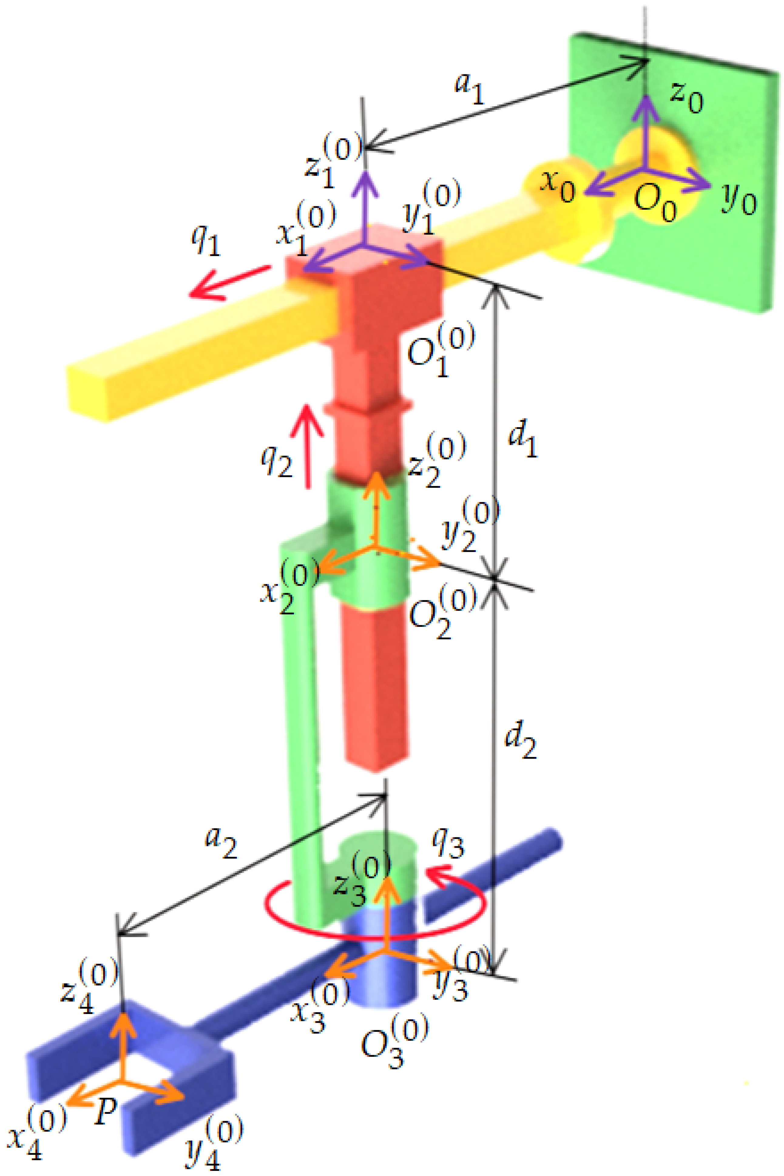
To illustrate the relation between the kinetic energy and acceleration energy of the first, second and third order, this section presented an application. For this purpose, the mechanical structure of a serial robot with three degrees of freedom, (2TR type), presented in
Figure 3, was considered. The kinematical structure of the considered robot was characterized by two prismatic joints (the first two joints) and a rotational joint (the last one). The robot structure, symbolized in
Figure 3, was modeled for the purpose of being implemented in the technological process of hot rolling and the processing of pipes by using any other methods than welding.
Based on the geometric and kinematic data contained in
Figure 3, and by using the expression (27), the kinetic energy of the robot 2TR structure was obtained:
In the expression (69), index denotes the sequence of the working process in which the robot is implemented and is the total number of working sequences. In the same expression, index represents the number of intervals corresponding to each sequence of the working process and is the time variable.
To improve the computation accuracy, each working sequence had to contain more than three intervals. In expression (69), and represent the masses of the robot’s kinetic links, and are the generalized coordinates from each robot joint and represents the distance from the geometrical center of the third joint and the characteristic point P, also considered in the geometric center of the robot end effector.
According to [
2], the generalized coordinates are functions of time and can define a rotation angle (in the case of rotational joints) or a linear displacement (for the prismatic joints). Using the general expression (41) and by performing some successive transformations, the acceleration energy of first order for the 2TR robot structure was obtained:
The significance of the terms contained in (70) was explained in the previous sections. Customizing relation (54), and by applying differential transformations, the expressions for the acceleration energies of second and third order were determined:
Using (69) and (70) by applying the second-order time derivative on expression (69) along with the restrictive condition (56), the identity was verified:
Thus, the mathematical relation between the kinetic energy and acceleration energy of first order was validated.
Expression (73) validates the demonstrations presented in the previous sections regarding the mathematical relation that could be established between the kinetic energy and acceleration energy of first order. This relation represents another approach that could be used in the dynamic study of mechanical systems.
For the graphical representation of the variation in time, in the case of the kinetic (
) and acceleration energy (
), for the generalized variables, the interpolation polynomial functions were used. Based on these functions, the generalized variables became time functions. For the serial robot structure presented in
Figure 3, a work process was modeled from which the motion trajectory was determined. In the case of industrial robots, the motion trajectory was defined as the reunion of all polynomial interpolation functions characterizing all selected time intervals and sequences of the working process. The simulated work process required the functioning of all three robot joints.
To achieve this goal, according to [
11], a linear interpolation polynomial function corresponding to
was considered. This function had the following form:
By integrating the expression (74), it was obtained that is:
The integration constants
were obtained by applying the continuity conditions, on each time interval and for each work sequence:
where
represents the number of work sequences and
is the number of time intervals; each sequence was divided. In the application,
and
.
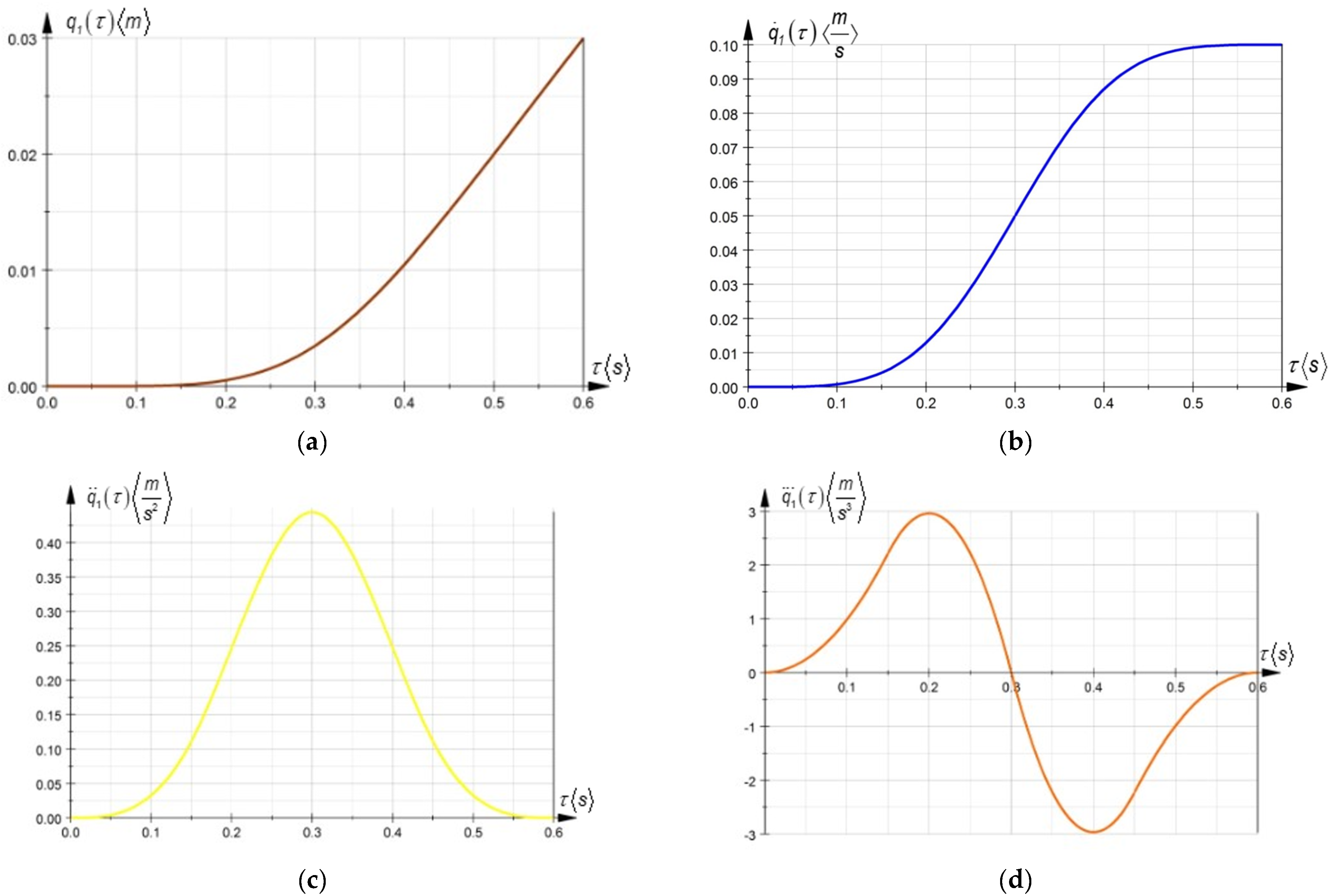
Thus, using a MATLAB application, the polynomial interpolation functions for each sequence and time interval were obtained. Further, we presented the interpolation functions corresponding to the first work sequence which was divided into four work intervals, according to
Table 1.
Based on the higher-order polynomial interpolation functions (5th order), presented in [
11], the variation of the generalized variables
and
was presented in a graphical form in
Figure 4.
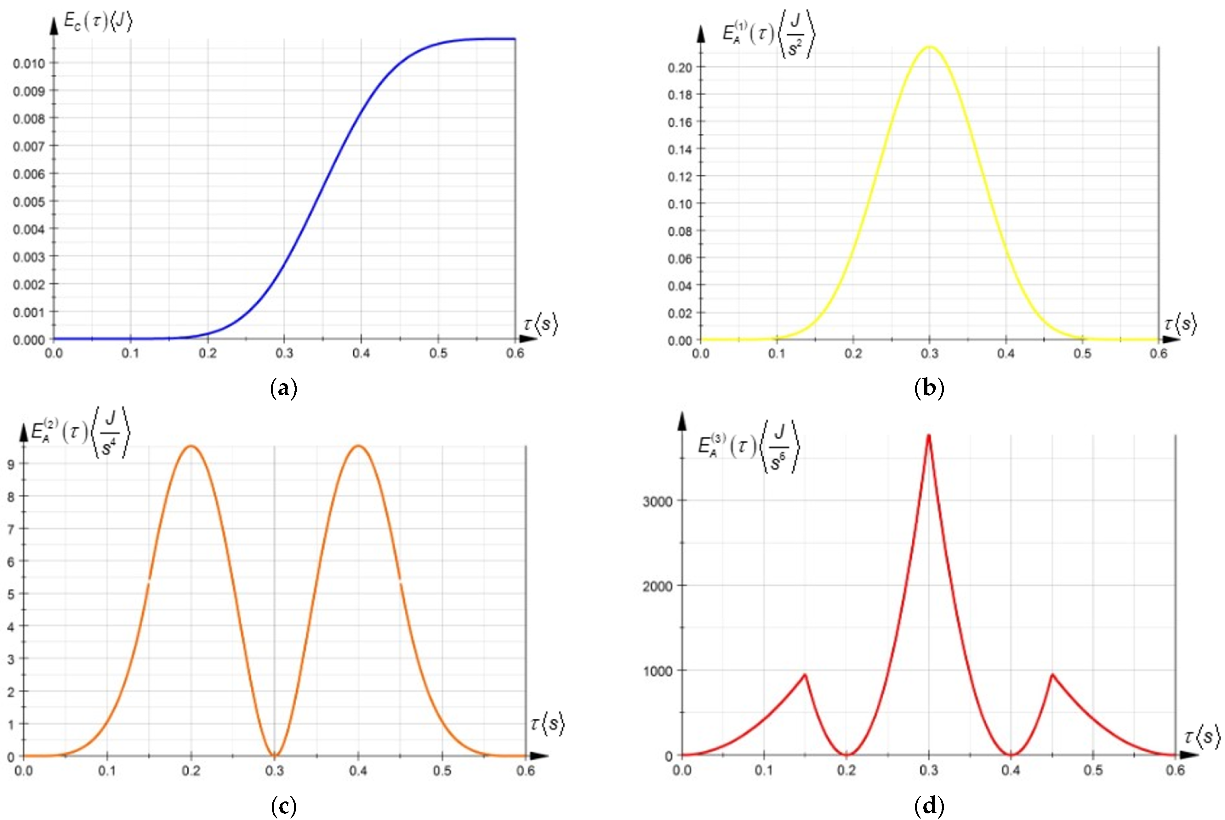
Figure 4 represents the variations in time of the generalized variables for a work sequence from the simulated work process. Substituting the results presented above in (69)–(72), the time variation laws for the kinetic energy and the acceleration energies of higher order were obtained. The variations are presented in
Figure 5.
The results presented above represent the compulsory input functions in the dynamic study of the robot mechanical structure, materialized by the time variation laws of the generalized driving forces as they resulted from the study encompassed in [
13].
7. Conclusions
In the industrial field, a wide range of applications is based on multibody mechanical systems, including, for example, parallel and serial robots. These multibody systems are characterized, in general, by rapid movements due to the active forces as time functions and due to the occurrence of higher-order accelerations within the mechanical system subjected to different technological processes.
This paper focused on establishing a mathematical relation between the kinetic energy and acceleration energy for different material systems that can be systems of material points, bodies and multibody systems. In terms of dynamics, higher-order accelerations became the central functions in acceleration energies. Generally, in advanced dynamics, the study of multibody systems is conducted by applying the differential and variational principles of analytical mechanics. Lagrange–Euler equations and their time derivatives are commonly used. In these types of equations, the central function becomes the kinetic energy and its higher-order time derivatives. The same study in advanced dynamics can be conducted by applying the generalization of the Gibbs–Appell equations, in which the central function becomes the first-order and higher-order acceleration energy.
To reach the main objective of the paper, in the second section, several formulations on kinetic energy were presented, while in the third section, the expression that defined the acceleration energy of first order, also known as Appell’s function, was presented in an explicit form. In the fourth section, the study then focused on extending the analysis of the acceleration energy of first order in the general case, with the purpose of establishing the higher-order equations in the dynamic behavior of the fast-moving mechanical systems. The next section, the fifth one, was dedicated to presenting the mathematical relations between the kinetic and acceleration energy in the case of a material point, of a discrete system of material points and of a multibody system. This section also encompassed a generalization of the differential study for advanced dynamics equations by presenting the mathematical relations between kinetic energy and its higher-order derivatives and the acceleration energy of higher order and its derivatives.
To illustrate the main results of the paper, namely, the mathematical relations between the kinetic energy and acceleration energy of the first, second and third order, an illustrative application was encompassed in the final part of the paper.


