
On Odd Perks-G Class of Distributions: Properties, Regression Model, Discretization, Bayesian and Non-Bayesian Estimation, and Applications

 ,
,  , and
, and 
Abstract
:1. Introduction
- (i)
- ;
- (ii)
- is differentiable and monotonically non-decreasing;
- (iii)
- as and as .
- (i)
- To realize special models for all sorts of HRFs;
- (ii)
- Under the same baseline distribution, to regularly provide better fits than alternative produced models;
- (iii)
- Compared to the baseline model, to increase the adjustability of the kurtosis;
- (iv)
- To construct symmetric, left- and right-skewed, and inverted J-shaped distributions.
2. Density of the - Class: Useful Expansions
2.1. Special Models
2.1.1. Odd Perks Uniform
2.1.2. Odd Perks Exponential
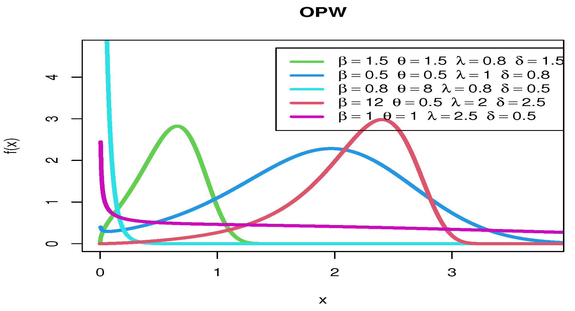
2.1.3. Odd Perks–Weibull
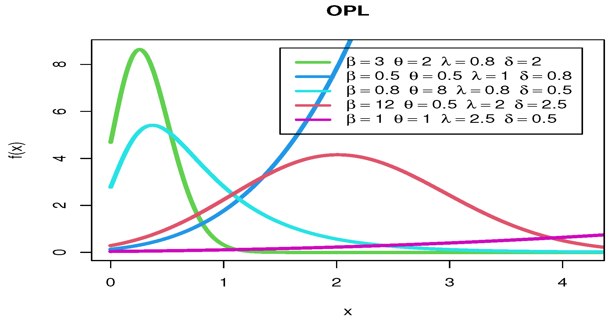
2.1.4. Odd Perks–Lomax
3. Statistical Features
3.1. Quantiles
3.2. Moments
3.3. Residual Lifetimes
3.4. Four Different Types of Entropy
4. Non-Bayesian Estimation
4.1. Likelihood Method
4.2. Maximum Product of Spacings (MPS) Estimation
5. Bayesian Estimation
- Sort the parameters as , , , and , where N is the length of the generated MCMC.
- The symmetric credible intervals for , and become , , and .
6. Bootstrap CI
- (i)
- Boot-p method
- (ii)
- Boot-t method
7. The Log-Odd Perks–Weibull Regression Model
MLE Method for Parameters of the Regression Model
8. Simulation Studies
8.1. Simulation for OPE Distribution
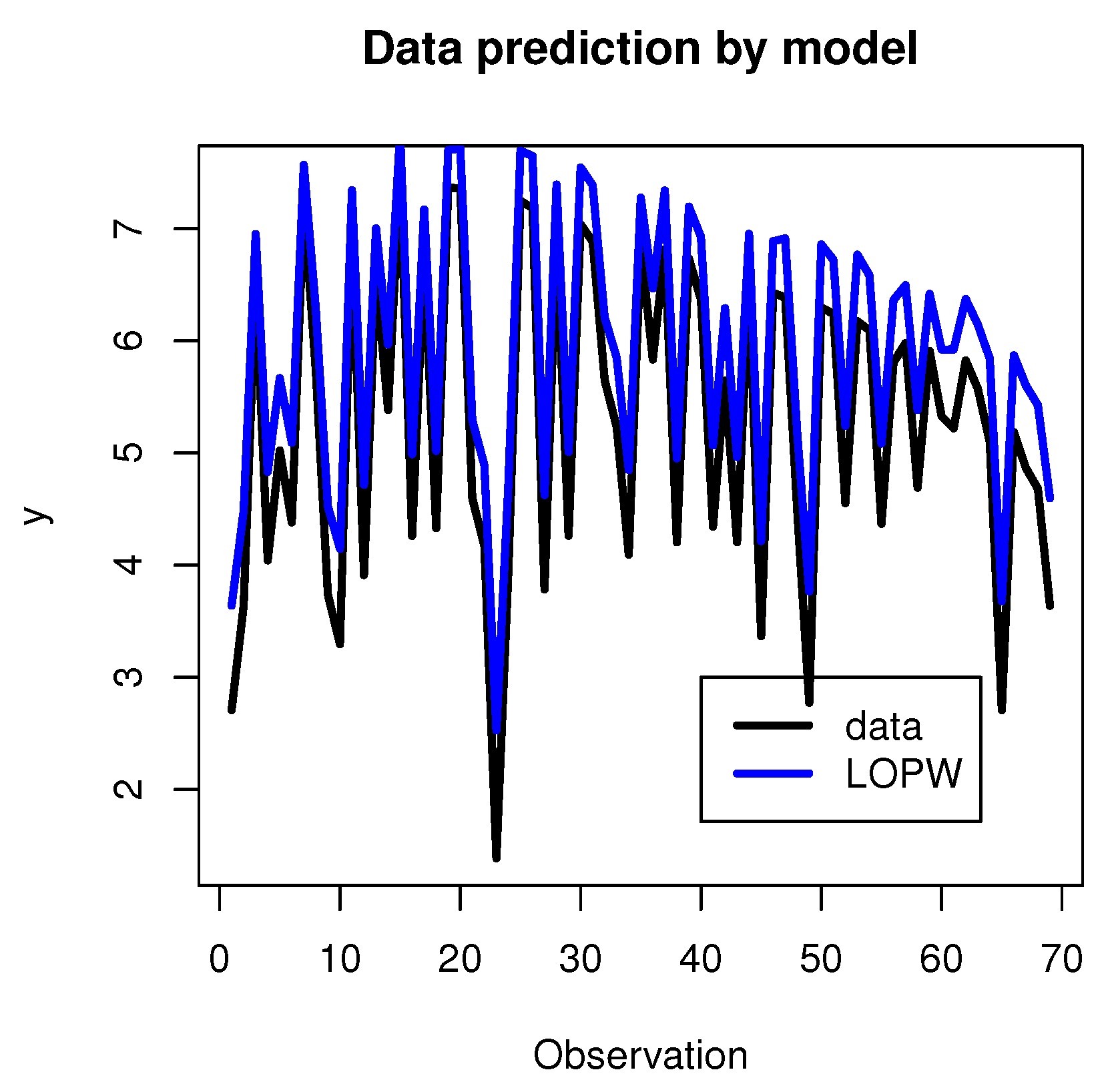
8.2. Simulation of the LOPW Regression Model
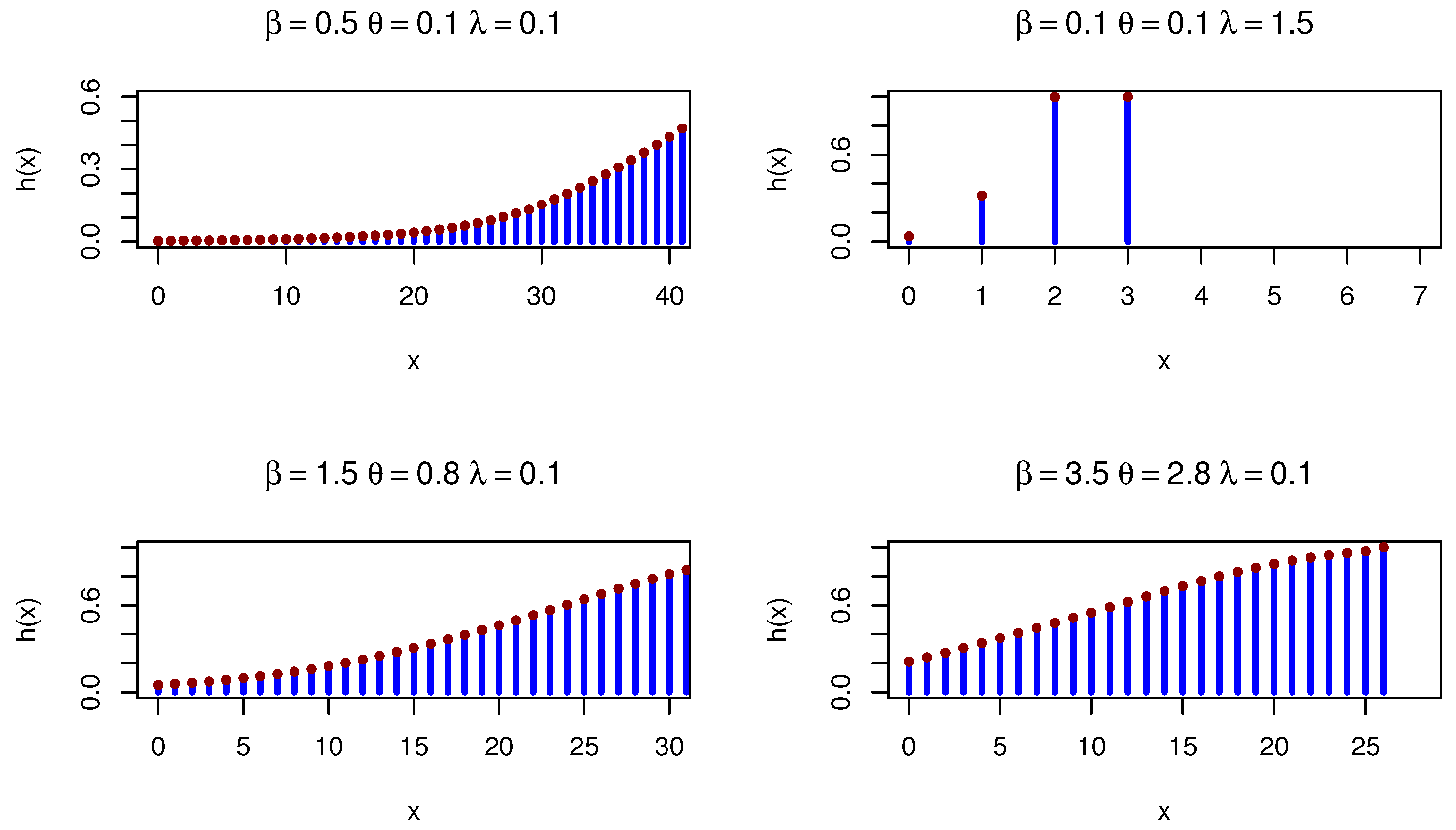
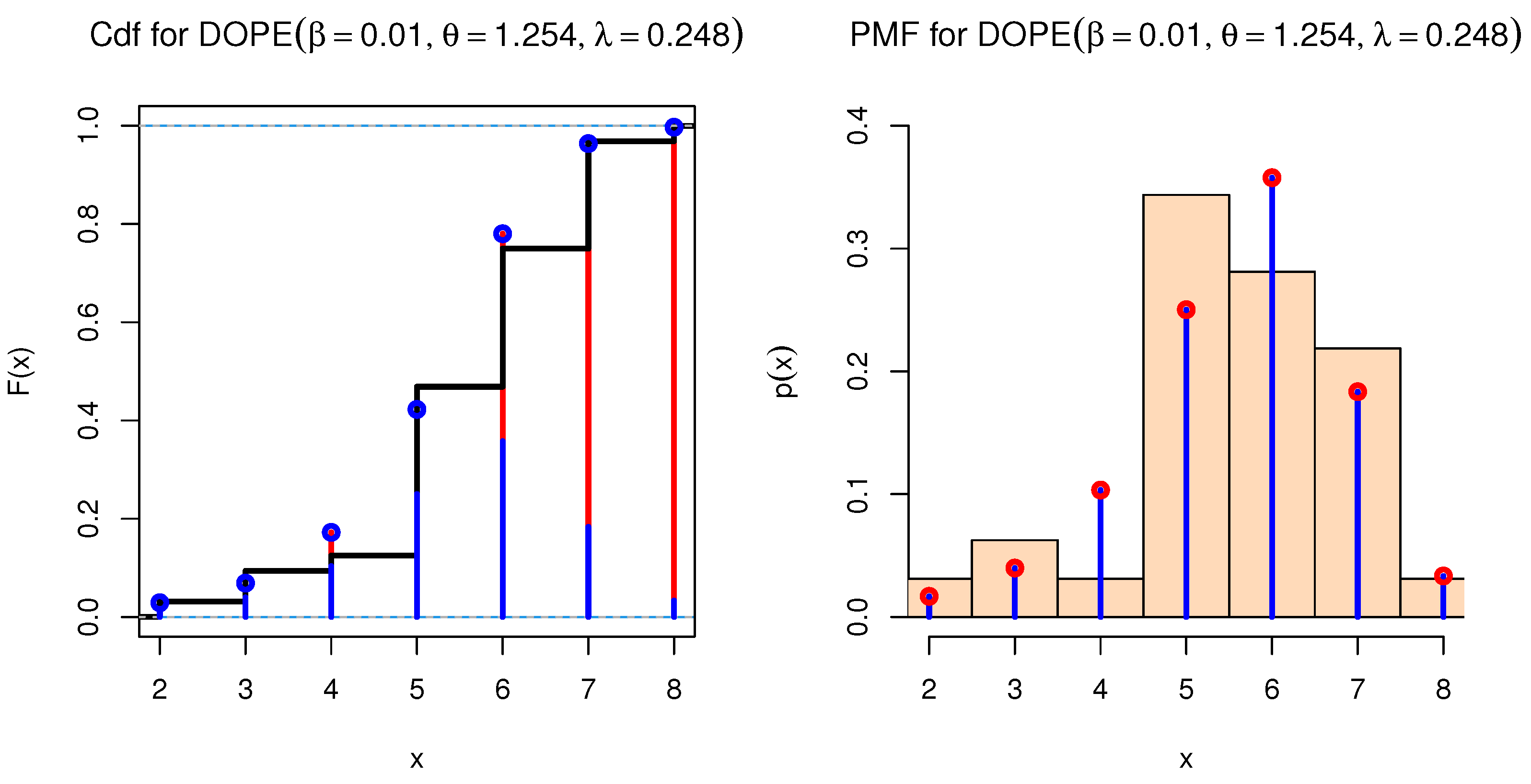
9. Discretization
10. Applications
10.1. Radiation Failure Mice
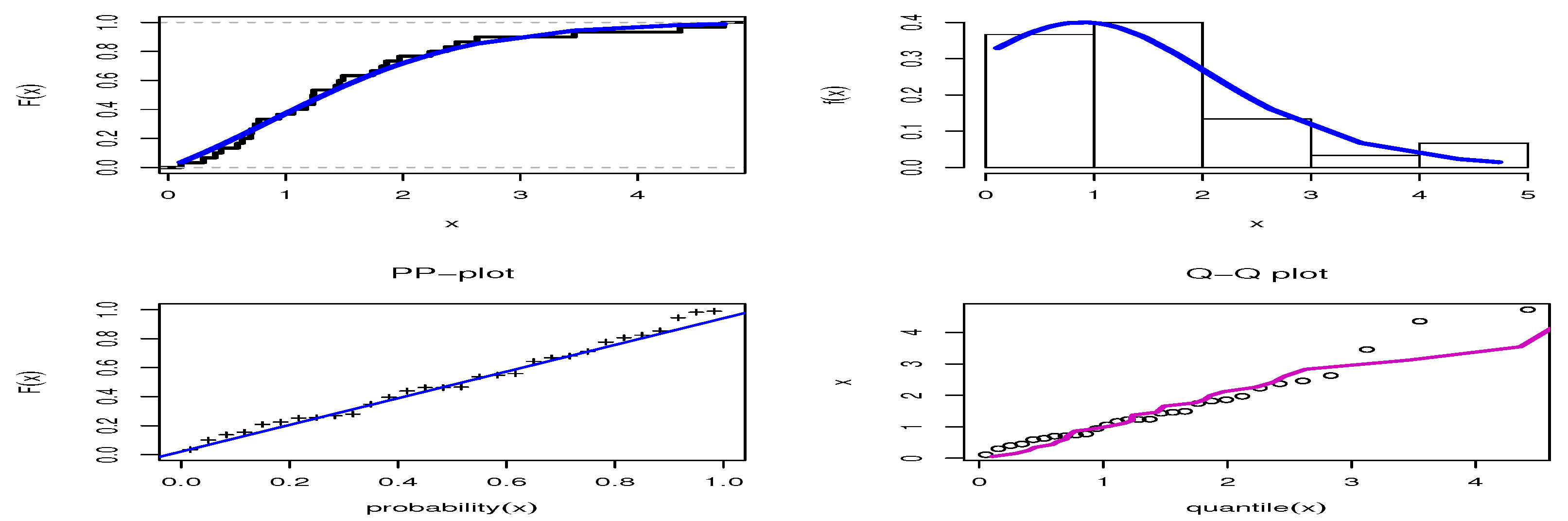
10.2. Failure Times of a Certain Product
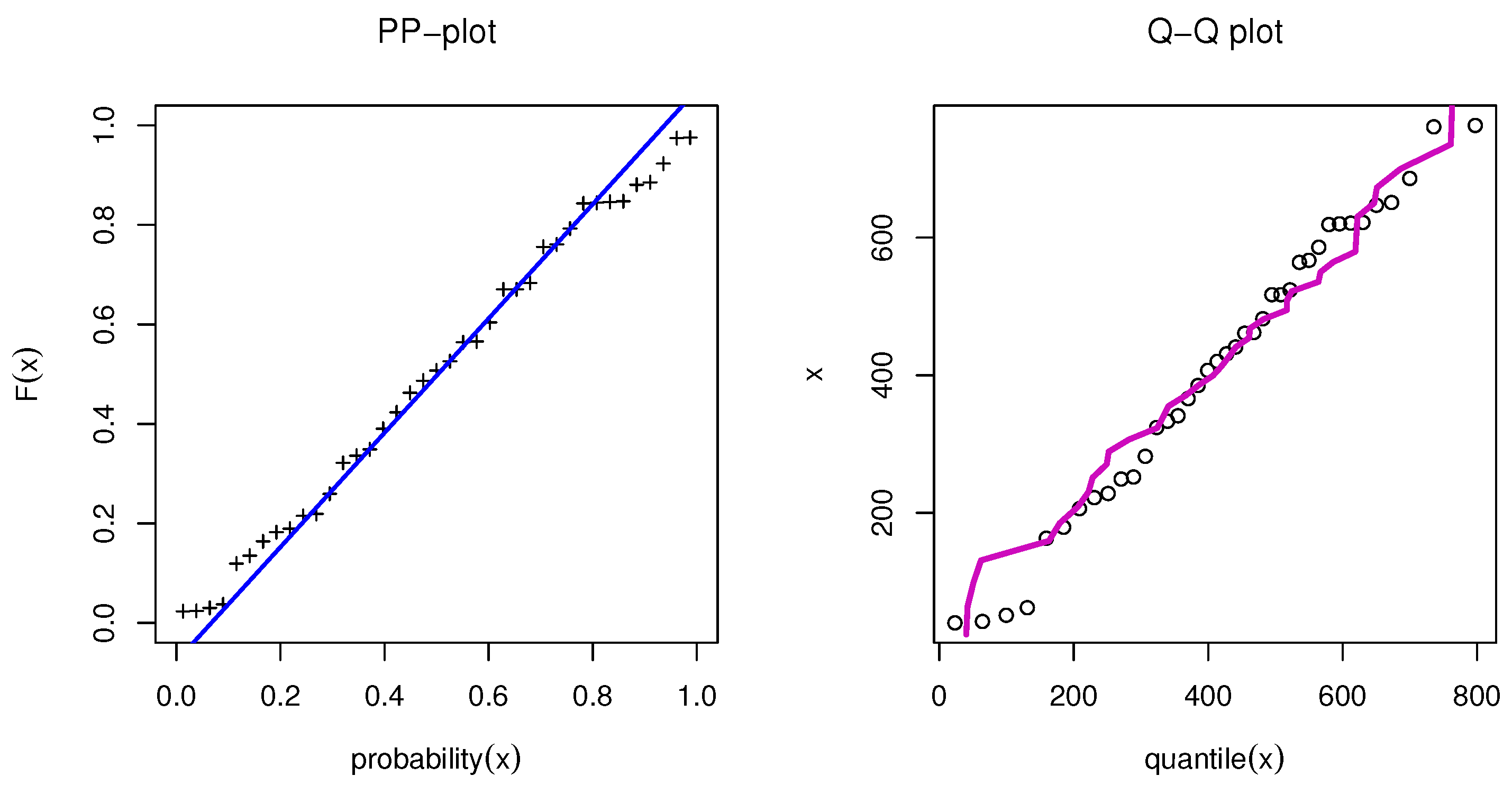
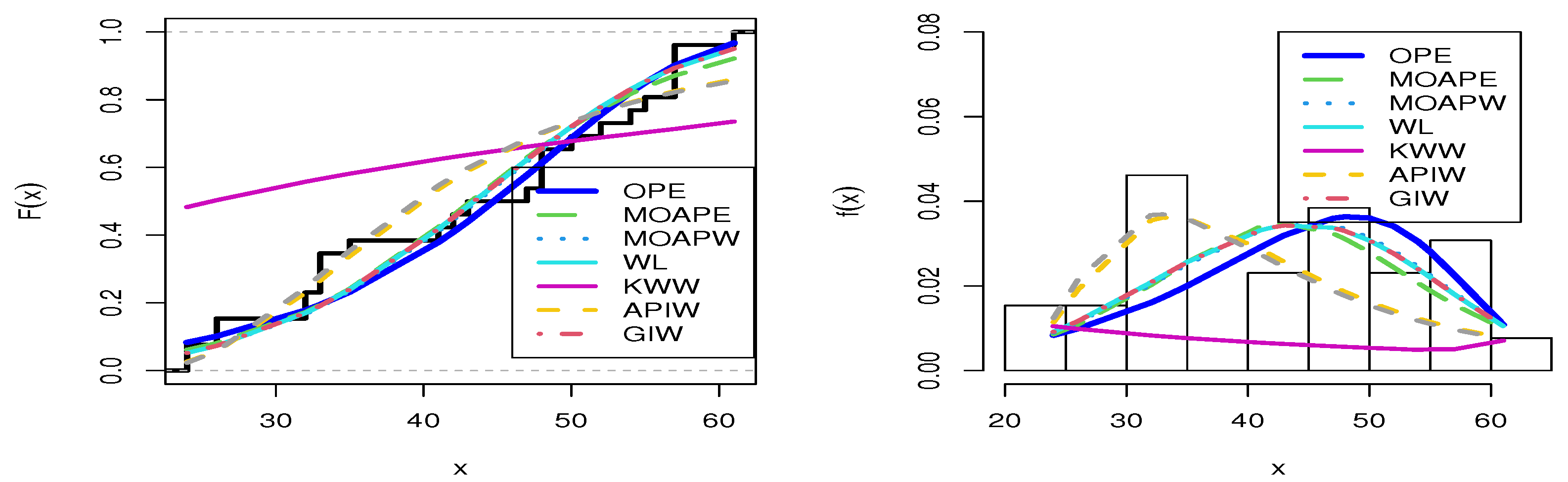
10.3. Mechanical Data
10.4. Stanford Heart Transplant Data
10.5. COVID-19 Data
11. Concluding Remarks
Author Contributions
Funding
Informed Consent Statement
Data Availability Statement
Conflicts of Interest
References
- Mudholkar, G.S.; Srivastava, D.K. Exponentiated Weibull family for analyzing bathtub failure-real data. IEEE Trans. Reliab. 1993, 42, 299–302. [Google Scholar] [CrossRef]
- Marshall, A.; Olkin, I. A new method for adding a parameter to a family of distributions with applications to the exponential and Weibull families. Biometrika 1997, 84, 641–652. [Google Scholar] [CrossRef]
- Alzaghal, A.; Famoye, F.; Lee, C. Exponentiated T-X Family of Distributions with Some Applications. Int. J. Stat. Probab. 2013, 3, 31–49. [Google Scholar] [CrossRef] [Green Version]
- Hassan, A.S.; Elgarhy, M.; Shakil, M. Type II half Logistic family of distributions with applications. Pak. J. Stat. Oper. Res. 2017, 13, 245–264. [Google Scholar]
- Bourguignon, M.; Silva, R.B.; Cordeiro, G.M. The Weibull-G family of probability distributions. J. Data Sci. 2014, 12, 1253–1268. [Google Scholar] [CrossRef]
- Eugene, N.; Lee, C.; Famoye, F. Beta-normal distribution and its applications. Commun. Stat. Theor. Methods 2002, 31, 497–512. [Google Scholar] [CrossRef]
- Zografos, K.; Balakrishnan, N. On families of beta-and generalized gamma-generated distributions and associated inference. Stat. Methodol. 2009, 6, 344–362. [Google Scholar] [CrossRef]
- Hassan, A.S.; Hemeda, S.E. The Additive Weibull-G Family of Probability Distributions. Int. J. Math. Its Appl. 2016, 4, 151–164. [Google Scholar]
- Gomes-Silva, F.S.; Percontini, A.; de Brito, E.; Ramos, M.W.; Venâncio, R.; Cordeiro, G.M. The odd Lindley-G family of distributions. Austrian J. Stat. 2017, 46, 65–87. [Google Scholar] [CrossRef] [Green Version]
- Al-Moisheer, A.S.; Elbatal, I.; Almutiry, W.; Elgarhy, M. Odd inverse power generalized Weibull generated family of distributions: Properties and applications. Math. Probl. Eng. 2021, 2021, 5082192. [Google Scholar] [CrossRef]
- Afify, A.Z.; Cordeiro, G.M.; Ibrahim, N.A.; Jamal, F.; Elgarhy, M.; Nasir, M.A. The Marshall-Olkin odd Burr III-G family: Theory, estimation, and engineering applications. IEEE Access 2021, 9, 4376–4387. [Google Scholar] [CrossRef]
- Al-Marzouki, S.; Jamal, F.; Chesneau, C.; Elgarhy, M. Topp-Leone odd Fréchet generated family of distributions with applications to COVID-19 data sets. Comput. Model. Eng. Sci. 2020, 125, 437–458. [Google Scholar]
- Badr, M.M.; Elbatal, I.; Jamal, F.; Chesneau, C.; Elgarhy, M. The transmuted odd Fréchet-G family of distributions: Theory and applications. Mathematics 2020, 8, 958. [Google Scholar] [CrossRef]
- Ahmad, Z.; Elgarhy, M.; Hamedani, G.G.; Butt, N.S. Odd generalized N-H generated family of distributions with application to exponential model. Pak. J. Stat. Oper. Res. 2020, 16, 53–71. [Google Scholar] [CrossRef]
- Haq, M.A.; Elgarhy, M.; Hashmi, S. The generalized odd Burr III family of distributions: Properties, applications and characterizations. J. Taibah Univ. Sci. 2019, 13, 961–971. [Google Scholar] [CrossRef] [Green Version]
- Haq, A.; Elgarhy, M. The odd Fréchet-G class of probability distributions. J. Stat. Appl. Probab. 2018, 7, 189–203. [Google Scholar] [CrossRef]
- Tahir, M.H.; Zubair, M.; Cordeiro, G.M.; Alzaatreh, A.; Mansoor, M. The Weibull-Power Cauchy Distribution: Model, Properties and Applications. Hacet. J. Math. Stat. 2017, 46, 767–789. [Google Scholar] [CrossRef]
- Cordeiro, G.; de Castro, M. A new family of generalized distributions. J. Stat. Comput. Simul. 2011, 81, 883–898. [Google Scholar] [CrossRef]
- Hassan, A.S.; Almetwally, E.M.; Ibrahim, G.M. Kumaraswamy inverted Topp–Leone distribution with applications to COVID-19 data. Comput. Mater. Contin. 2021, 68, 337–358. [Google Scholar] [CrossRef]
- Almetwally, E.M. The odd Weibull inverse topp–leone distribution with applications to COVID-19 data. Ann. Data Sci. 2022, 9, 121–140. [Google Scholar] [CrossRef]
- Nagy, M.; Almetwally, E.M.; Gemeay, A.M.; Mohammed, H.S.; Jawa, T.M.; Sayed-Ahmed, N.; Muse, A.H. The New Novel Discrete Distribution with Application on COVID-19 Mortality Numbers in Kingdom of Saudi Arabia and Latvia. Complexity 2021, 2021, 7192833. [Google Scholar] [CrossRef]
- Perks, W. On some experiments in the graduation of mortality statistics. J. Inst. Actuar. 1932, 43, 12–57. [Google Scholar] [CrossRef]
- Marshall, A.W.; Olkin, I. Life Distributions; Springer: New York, NY, USA, 2007; Volume 13. [Google Scholar]
- Richards, S.J. Applying survival models to pensioner mortality data. Br. Actuar. J. 2008, 14, 257–303. [Google Scholar] [CrossRef] [Green Version]
- Haberman, S.; Renshaw, A. A comparative study of parametric mortality projection models. Insur. Math. Econ. 2011, 48, 35–55. [Google Scholar] [CrossRef] [Green Version]
- Alzaatreh, A.; Lee, C.; Famoye, F. A new method for generating families of continuous distributions. Metron 2013, 71, 63–79. [Google Scholar] [CrossRef] [Green Version]
- Carrasco, J.M.; Ortega, E.M.; Paula, G.A. Log-modified Weibull regression models with censored data: Sensitivity and residual analysis. Comput. Stat. Data Anal. 2008, 52, 4021–4039. [Google Scholar] [CrossRef]
- Silva, G.O.; Ortega, E.M.; Cancho, V.G. Log-Weibull extended regression model: Estimation, sensitivity and residual analysis. Stat. Methodol. 2010, 7, 614–631. [Google Scholar] [CrossRef]
- Hashimoto, E.M.; Ortega, E.M.; Cordeiro, G.M.; Barreto, M.L. The Log-Burr XII regression model for grouped survival data. J. Biopharm. Stat. 2012, 22, 141–159. [Google Scholar] [CrossRef]
- Ortega, E.M.; Cordeiro, G.M.; Kattan, M.W. The log-beta Weibull regression model with application to predict recurrence of prostate cancer. Stat. Pap. 2013, 54, 113–132. [Google Scholar] [CrossRef]
- Alamoudi, H.H.; Mousa, S.A.; Baharith, L.A. Estimation and application in log-Fréchet regression model using censored data. Int. J. Adv. Stat. Probab. 2017, 5, 23–31. [Google Scholar] [CrossRef] [Green Version]
- Baharith, L.A.; Al-Beladi, K.M.; Klakattawi, H.S. The Odds Exponential-Pareto IV Distribution: Regression Model and Application. Entropy 2020, 22, 497. [Google Scholar] [CrossRef] [PubMed]
- Rényi, A. On measures of entropy and information. In Proceedings of the 4th Berkeley Symposium on Mathematical Statistics and Probability, Berkeley, CA, USA, 20–30 June 1960; Volume 1, pp. 47–561. [Google Scholar]
- Tsallis, C. Possible generalization of Boltzmann-Gibbs statistics. J. Stat. Phys. 1988, 52, 479–487. [Google Scholar] [CrossRef]
- Havrda, J.; Charvat, F. Quantification method of classification processes, concept of structural a-entropy. Kybernetika 1967, 3, 30–35. [Google Scholar]
- Arimoto, S. Information-theoretical considerations on estimation problems. Inf. Control. 1971, 19, 181–194. [Google Scholar] [CrossRef] [Green Version]
- Cheng, R.C.H.; Amin, N.A.K. Estimating parameters in continuous univariate distributions with a shifted origin. J. R. Stat. Soc. Ser. B (Methodol.) 1983, 45, 394–403. [Google Scholar] [CrossRef]
- Ranneby, B. The maximum spacing method. An estimation method related to the maximum likelihood method. Scand. J. Stat. 1984, 11, 93–112. [Google Scholar]
- Chen, M.H.; Shao, Q.M. Monte Carlo estimation of Bayesian credible and HPD intervals. J. Comput. Graph. Stat. 1999, 8, 69–92. [Google Scholar]
- Efron, B.; Tibshirani, R.J. An Introduction to the Bootstrap; CRC Press: Boca Raton, FL, USA, 1994. [Google Scholar]
- Hall, P. Theoretical comparison of bootstrap confidence intervals. Ann. Stat. 1988, 16, 927–953. [Google Scholar] [CrossRef]
- Muhammed, H.Z.; Almetwally, E.M. Bayesian and non-Bayesian estimation for the bivariate inverse weibull distribution under progressive type-II censoring. Ann. Data Sci. 2020, 1–32. [Google Scholar] [CrossRef]
- Nassr, S.G.; Almetwally, E.M.; El Azm, W.S.A. Statistical inference for the extended weibull distribution based on adaptive type-II progressive hybrid censored competing risks data. Thail. Stat. 2021, 19, 547–564. [Google Scholar]
- Almongy, H.M.; Almetwally, E.M.; Alharbi, R.; Alnagar, D.; Hafez, E.H.; El-Din, M.M.M. The Weibull generalized exponential distribution with censored sample: Estimation and application on real data. Complexity 2021, 2021, 6653534. [Google Scholar] [CrossRef]
- Roy, D. Discrete Rayleigh distribution. IEEE Trans. Reliab. 2004, 53, 255–260. [Google Scholar] [CrossRef]
- Nassar, M.; Kumar, D.; Dey, S.; Cordeiro, G.M.; Afify, A.Z. The Marshall–Olkin alpha power family of distributions with applications. J. Comput. Appl. Math. 2019, 351, 41–53. [Google Scholar] [CrossRef]
- Almetwally, E.M.; Sabry, M.A.; Alharbi, R.; Alnagar, D.; Mubarak, S.A.; Hafez, E.H. Marshall–Olkin alpha power weibull distribution: Different methods of estimation based on type-I and type-II censoring. Complexity 2021, 2021, 5533799. [Google Scholar] [CrossRef]
- Tahir, M.H.; Cordeiro, G.M.; Mansoor, M.; Zubair, M. The Weibull-Lomax distribution: Properties and applications. Hacet. J. Math. Stat. 2015, 44, 461–480. [Google Scholar] [CrossRef]
- Cordeiro, G.M.; Ortega, E.M.; Nadarajah, S. The Kumaraswamy Weibull distribution with application to failure data. J. Frankl. Inst. 2010, 347, 1399–1429. [Google Scholar] [CrossRef]
- Basheer, A.M. Alpha power inverse Weibull distribution with reliability application. J. Taibah Univ. Sci. 2019, 13, 423–432. [Google Scholar] [CrossRef] [Green Version]
- De Gusmao, F.R.; Ortega, E.M.; Cordeiro, G.M. The generalized inverse Weibull distribution. Stat. Pap. 2011, 52, 591–619. [Google Scholar] [CrossRef]
- Gacula, M.C., Jr.; Kubala, J.J. Statistical models for shelf life failures. J. Food Sci. 1975, 40, 404–409. [Google Scholar] [CrossRef]
- Seber, G.A.; Wild, C.J. Wiley Series in Probability and Statistics. Linear Regression Analysis; Wiley: Hoboken, NJ, USA, 2003; pp. 36–44. [Google Scholar]
- Elshahhat, A.; Aljohani, H.M.; Afify, A.Z. Bayesian and Classical Inference under Type-II Censored Samples of the Extended Inverse Gompertz Distribution with Engineering Applications. Entropy 2021, 23, 1578. [Google Scholar] [CrossRef]
- Kalbfleisch, J.D.; Prentice, R.L. The Statistical Analysis of Failure Time Data; John Wiley & Sons: Hoboken, NJ, USA, 2011; Volume 360. [Google Scholar]
- Almetwally, E.M.; Abdo, D.A.; Hafez, E.H.; Jawa, T.M.; Sayed-Ahmed, N.; Almongy, H.M. The new discrete distribution with application to COVID-19 Data. Results Phys. 2022, 32, 104987. [Google Scholar] [CrossRef] [PubMed]
- Krishna, H.; Pundir, P.S. Discrete Burr and discrete Pareto distributions. Stat. Methodol. 2009, 6, 177–188. [Google Scholar] [CrossRef]
- Jazi, M.A.; Lai, C.D.; Alamatsaz, M.H. A discrete inverse Weibull distribution and estimation of its parameters. Stat. Methodol. 2010, 7, 121–132. [Google Scholar] [CrossRef]
- Fisher, P. Negative Binomial Distribution. Ann. Eugen. 1941, 11, 182–787. [Google Scholar] [CrossRef]
- Nekoukhou, V.; Alamatsaz, M.H.; Bidram, H. Discrete generalized exponential distribution of a second type. Statistics 2013, 47, 876–887. [Google Scholar] [CrossRef]
- Almetwally, E.M.; Ibrahim, G.M. Discrete alpha power inverse Lomax distribution with application of COVID-19 data. Int. J. Appl. Math. 2020, 9, 11–22. [Google Scholar]
- Gómez-Déniz, E.; Calderín-Ojeda, E. The discrete Lindley distribution: Properties and applications. J. Stat. Comput. Simul. 2011, 81, 1405–1416. [Google Scholar] [CrossRef]
- Eldeeb, A.S.; Ahsan-Ul-Haq, M.; Babar, A. A discrete analog of inverted Topp-Leone distribution: Properties, estimation and applications. Int. J. Anal. Appl. 2021, 19, 695–708. [Google Scholar]
- Nekoukhou, V.; Bidram, H. The exponentiated discrete Weibull distribution. Sort 2015, 39, 127–146. [Google Scholar]
- Almetwally, E.M.; Almongy, H.M.; Saleh, H.A. Managing risk of spreading “COVID-19” in Egypt: Modelling using a discrete Marshall-Olkin generalized exponential distribution. Int. J. Probab. Stat. 2020, 9, 33–41. [Google Scholar]


| Var | SK | KU | CV | |||||
|---|---|---|---|---|---|---|---|---|
| 0.5, 0.5, 0.5 | 2.523 | 7.741 | 26.091 | 93.614 | 1.373 | −0.23 | 2.312 | 0.464 |
| 0.8, 0.5, 0.5 | 2.344 | 6.863 | 22.392 | 78.425 | 1.369 | −0.071 | 2.224 | 0.499 |
| 1.2, 0.5, 0.5 | 2.214 | 6.26 | 19.944 | 68.654 | 1.359 | 0.042 | 2.205 | 0.527 |
| 1.5, 0.5, 0.5 | 2.153 | 5.987 | 18.861 | 64.406 | 1.353 | 0.094 | 2.207 | 0.54 |
| 2.0, 0.5, 0.5 | 2.085 | 5.691 | 17.706 | 59.929 | 1.343 | 0.153 | 2.219 | 0.556 |
| 2.5, 0.5, 0.5 | 2.041 | 5.501 | 16.974 | 57.123 | 1.336 | 0.191 | 2.232 | 0.566 |
| 3.0, 0.5, 0.5 | 2.01 | 5.369 | 16.469 | 55.197 | 1.33 | 0.218 | 2.244 | 0.574 |
| 0.5, 0.8, 0.5 | 1.989 | 4.938 | 13.777 | 41.633 | 0.982 | 0.049 | 2.373 | 0.498 |
| 0.5, 1.2, 0.5 | 1.552 | 3.099 | 7.081 | 17.749 | 0.692 | 0.216 | 2.477 | 0.536 |
| 0.5, 1.5, 0.5 | 1.339 | 2.349 | 4.76 | 10.658 | 0.556 | 0.304 | 2.558 | 0.557 |
| 0.5, 2.0, 0.5 | 1.096 | 1.609 | 2.765 | 5.303 | 0.408 | 0.415 | 2.698 | 0.583 |
| 0.5, 2.5, 0.5 | 0.931 | 1.18 | 1.771 | 2.989 | 0.314 | 0.499 | 2.834 | 0.602 |
| 0.5, 3.0, 0.5 | 0.81 | 0.907 | 1.211 | 1.832 | 0.25 | 0.567 | 2.96 | 0.618 |
| 0.5, 0.5, 0.8 | 1.614 | 3.145 | 6.774 | 15.629 | 0.541 | −0.12 | 2.405 | 0.456 |
| 0.5, 0.5, 1.2 | 1.076 | 1.398 | 2.007 | 3.087 | 0.24 | −0.12 | 2.405 | 0.456 |
| REN | TEN | HCEN | AEN | REN | TEN | HCEN | AEN | REN | TEN | HCEN | AEN | |
|---|---|---|---|---|---|---|---|---|---|---|---|---|
| 0.5, 0.5, 0.5 | 0.669 | 2.802 | 3.669 | 2.322 | 0.651 | 1.8 | 1.179 | 1.054 | 0.618 | 1.364 | 0.957 | 0.588 |
| 0.8, 0.5, 0.5 | 0.671 | 2.812 | 3.686 | 2.329 | 0.652 | 1.803 | 1.181 | 1.056 | 0.626 | 1.369 | 0.965 | 0.59 |
| 1.2, 0.5, 0.5 | 0.669 | 2.804 | 3.671 | 2.323 | 0.649 | 1.797 | 1.177 | 1.053 | 0.626 | 1.369 | 0.965 | 0.59 |
| 1.5, 0.5, 0.5 | 0.668 | 2.795 | 3.657 | 2.316 | 0.646 | 1.792 | 1.173 | 1.05 | 0.624 | 1.368 | 0.963 | 0.59 |
| 2.0, 0.5, 0.5 | 0.666 | 2.783 | 3.635 | 2.306 | 0.642 | 1.784 | 1.167 | 1.045 | 0.621 | 1.366 | 0.96 | 0.589 |
| 2.5, 0.5, 0.5 | 0.664 | 2.774 | 3.618 | 2.298 | 0.639 | 1.778 | 1.163 | 1.041 | 0.618 | 1.364 | 0.957 | 0.588 |
| 3.0, 0.5, 0.5 | 0.663 | 2.766 | 3.604 | 2.291 | 0.636 | 1.773 | 1.159 | 1.039 | 0.616 | 1.362 | 0.955 | 0.587 |
| 0.5, 0.8, 0.5 | 0.628 | 2.563 | 3.25 | 2.123 | 0.575 | 1.652 | 1.07 | 0.968 | 0.549 | 1.315 | 0.886 | 0.567 |
| 0.5, 1.2, 0.5 | 0.557 | 2.169 | 2.604 | 1.797 | 0.494 | 1.481 | 0.946 | 0.867 | 0.47 | 1.242 | 0.796 | 0.535 |
| 0.5, 1.5, 0.5 | 0.509 | 1.925 | 2.23 | 1.595 | 0.442 | 1.363 | 0.864 | 0.798 | 0.419 | 1.183 | 0.732 | 0.51 |
| 0.5, 2.0, 0.5 | 0.442 | 1.6 | 1.765 | 1.325 | 0.369 | 1.181 | 0.74 | 0.692 | 0.344 | 1.076 | 0.631 | 0.464 |
| 0.5, 2.5, 0.5 | 0.385 | 1.345 | 1.425 | 1.114 | 0.306 | 1.014 | 0.628 | 0.594 | 0.281 | 0.96 | 0.536 | 0.414 |
| 0.5, 3.0, 0.5 | 0.335 | 1.137 | 1.164 | 0.942 | 0.252 | 0.859 | 0.527 | 0.503 | 0.225 | 0.836 | 0.445 | 0.36 |
| 0.5, 0.5, 0.8 | 0.507 | 1.914 | 2.214 | 1.585 | 0.444 | 1.366 | 0.866 | 0.8 | 0.414 | 1.177 | 0.726 | 0.507 |
| 0.5, 0.5, 1.2 | 0.331 | 1.12 | 1.143 | 0.927 | 0.268 | 0.906 | 0.558 | 0.531 | 0.238 | 0.866 | 0.467 | 0.373 |
| MLE | MPS | Bayesian | ||||||||||||
|---|---|---|---|---|---|---|---|---|---|---|---|---|---|---|
| n | Bias | MSE | L.CI | L.BP | L.BT | Bias | MSE | L.CI | Bias | MSE | L.CI | |||
| 0.5 | 0.6 | 30 | 0.0446 | 0.0554 | 0.9067 | 0.0289 | 0.0297 | 0.0979 | 0.0812 | 0.9959 | 0.1079 | 0.0528 | 0.7230 | |
| −0.0009 | 0.0396 | 0.7808 | 0.0243 | 0.0243 | 0.1134 | 0.0715 | 0.8355 | 0.0660 | 0.0741 | 0.9372 | ||||
| 0.0353 | 0.0147 | 0.4541 | 0.0152 | 0.0152 | −0.0398 | 0.0137 | 0.5062 | 0.0259 | 0.0175 | 0.4776 | ||||
| 70 | 0.0045 | 0.0129 | 0.4455 | 0.0142 | 0.0143 | 0.0405 | 0.0302 | 0.6271 | 0.0663 | 0.0318 | 0.6188 | |||
| 0.0023 | 0.0116 | 0.4225 | 0.0132 | 0.0133 | 0.0619 | 0.0258 | 0.5218 | 0.0322 | 0.0397 | 0.7238 | ||||
| 0.0116 | 0.0048 | 0.2690 | 0.0088 | 0.0088 | −0.0256 | 0.0057 | 0.3164 | 0.0168 | 0.0099 | 0.3732 | ||||
| 150 | 0.0107 | 0.0107 | 0.4038 | 0.0132 | 0.0135 | 0.0151 | 0.0140 | 0.4563 | 0.0251 | 0.0149 | 0.4517 | |||
| 0.0049 | 0.0159 | 0.4934 | 0.0159 | 0.0157 | 0.0361 | 0.0119 | 0.3719 | 0.0090 | 0.0150 | 0.4616 | ||||
| 0.0091 | 0.0042 | 0.2505 | 0.0079 | 0.0078 | −0.0154 | 0.0027 | 0.2183 | 0.0094 | 0.0037 | 0.2304 | ||||
| 3 | 30 | 0.0578 | 0.1240 | 1.3625 | 0.0437 | 0.0437 | 0.1456 | 0.1497 | 1.3182 | 0.0887 | 0.0453 | 0.6658 | ||
| 0.0639 | 0.0623 | 0.9462 | 0.0317 | 0.0318 | 0.1182 | 0.0805 | 0.9572 | 0.0635 | 0.0350 | 0.6478 | ||||
| 0.0103 | 0.1448 | 1.4920 | 0.0479 | 0.0470 | −0.2354 | 0.2201 | 1.8373 | −0.0341 | 0.1352 | 1.3905 | ||||
| 70 | 0.0319 | 0.0566 | 0.9248 | 0.0302 | 0.0303 | 0.0450 | 0.0533 | 0.8748 | 0.0521 | 0.0305 | 0.5807 | |||
| 0.0425 | 0.0454 | 0.8185 | 0.0254 | 0.0256 | 0.0873 | 0.0448 | 0.7118 | 0.0360 | 0.0191 | 0.5039 | ||||
| 0.0161 | 0.1114 | 1.3074 | 0.0410 | 0.0406 | −0.1550 | 0.1214 | 1.3947 | −0.0133 | 0.0746 | 1.0636 | ||||
| 150 | 0.0182 | 0.0340 | 0.7191 | 0.0237 | 0.0238 | 0.0298 | 0.0281 | 0.6348 | 0.0127 | 0.0118 | 0.3992 | |||
| 0.0411 | 0.0344 | 0.7097 | 0.0221 | 0.0221 | 0.0525 | 0.0219 | 0.5317 | 0.0150 | 0.0059 | 0.2762 | ||||
| −0.0204 | 0.0703 | 1.0365 | 0.0349 | 0.0349 | −0.0972 | 0.0632 | 0.9861 | −0.0007 | 0.0249 | 0.6179 | ||||
| 2 | 0.6 | 30 | 0.0425 | 0.0994 | 1.2251 | 0.0398 | 0.0400 | 0.1859 | 0.1904 | 1.4047 | 0.0869 | 0.0384 | 0.6382 | |
| −0.0429 | 0.0856 | 1.1353 | 0.0382 | 0.0382 | 0.0509 | 0.0773 | 0.9783 | −0.0216 | 0.0803 | 1.2539 | ||||
| 0.0405 | 0.0134 | 0.4260 | 0.0130 | 0.0129 | −0.0251 | 0.0107 | 0.4585 | 0.0267 | 0.0117 | 0.3827 | ||||
| 70 | 0.0478 | 0.0606 | 0.9473 | 0.0310 | 0.0308 | 0.0983 | 0.0466 | 0.8826 | 0.0619 | 0.0263 | 0.5548 | |||
| −0.0412 | 0.0893 | 1.1611 | 0.0367 | 0.0365 | 0.0494 | 0.0321 | 0.5847 | −0.0118 | 0.0790 | 1.1261 | ||||
| 0.0241 | 0.0074 | 0.3248 | 0.0101 | 0.0101 | −0.0208 | 0.0043 | 0.2886 | 0.0141 | 0.0059 | 0.2877 | ||||
| 150 | 0.0116 | 0.0153 | 0.4822 | 0.0150 | 0.0150 | 0.0502 | 0.0120 | 0.5232 | 0.0216 | 0.0118 | 0.3925 | |||
| 0.0019 | 0.0037 | 0.2386 | 0.0072 | 0.0072 | 0.0305 | 0.0133 | 0.4067 | −0.0155 | 0.0037 | 0.2062 | ||||
| 0.0037 | 0.0015 | 0.1490 | 0.0048 | 0.0048 | −0.0146 | 0.0019 | 0.1802 | 0.0073 | 0.0011 | 0.1372 | ||||
| 3 | 30 | 0.3058 | 0.7826 | 3.2557 | 0.1044 | 0.1042 | 0.2925 | 0.3949 | 2.1947 | 0.1068 | 0.0491 | 0.6704 | ||
| −0.1049 | 0.6079 | 3.0301 | 0.0951 | 0.0941 | 0.0830 | 0.2070 | 1.5667 | 0.0095 | 0.1283 | 1.3565 | ||||
| 0.3745 | 0.6661 | 2.8440 | 0.0907 | 0.0910 | −0.1532 | 0.2509 | 2.3979 | 0.0176 | 0.1194 | 1.3171 | ||||
| 70 | 0.1345 | 0.6876 | 3.2091 | 0.1065 | 0.0947 | 0.1228 | 0.1015 | 1.1647 | 0.0643 | 0.0266 | 0.5542 | |||
| −0.0322 | 0.3965 | 2.4663 | 0.0797 | 0.0799 | 0.0900 | 0.1366 | 1.2837 | 0.0154 | 0.0759 | 1.0942 | ||||
| 0.1747 | 0.3802 | 2.3193 | 0.0741 | 0.0736 | −0.1296 | 0.1323 | 1.6370 | −0.0014 | 0.0615 | 0.9628 | ||||
| 150 | 0.0776 | 0.0719 | 1.0063 | 0.0323 | 0.0331 | 0.0566 | 0.0338 | 0.7071 | 0.0225 | 0.0109 | 0.3860 | |||
| −0.0590 | 0.2817 | 2.0688 | 0.0605 | 0.0595 | 0.0586 | 0.0757 | 0.9369 | 0.0111 | 0.0215 | 0.5600 | ||||
| 0.1491 | 0.2541 | 1.8886 | 0.0602 | 0.0605 | −0.0759 | 0.0642 | 1.1735 | 0.0010 | 0.0210 | 0.5712 | ||||
| MLE | MPS | Bayesian | ||||||||||||
|---|---|---|---|---|---|---|---|---|---|---|---|---|---|---|
| n | Bias | MSE | L.CI | L.BP | L.BT | Bias | MSE | L.CI | Bias | MSE | L.CI | |||
| 0.5 | 0.6 | 30 | 0.0353 | 0.0964 | 1.2101 | 0.0408 | 0.0403 | 0.0199 | 0.0124 | 0.4456 | 0.0118 | 0.0377 | 0.7393 | |
| −0.0025 | 0.0921 | 1.1901 | 0.0377 | 0.0367 | 0.1384 | 0.0910 | 1.1635 | 0.0749 | 0.0718 | 0.9038 | ||||
| 0.0731 | 0.0398 | 0.7277 | 0.0230 | 0.0230 | −0.0288 | 0.0279 | 0.7468 | 0.0237 | 0.0198 | 0.5344 | ||||
| 70 | 0.0270 | 0.0426 | 0.8021 | 0.0268 | 0.0267 | 0.0092 | 0.0048 | 0.2881 | 0.0003 | 0.0343 | 0.7287 | |||
| 0.0007 | 0.0455 | 0.8363 | 0.0264 | 0.0264 | 0.0778 | 0.0543 | 0.7847 | 0.0345 | 0.0367 | 0.7005 | ||||
| 0.0311 | 0.0157 | 0.4759 | 0.0152 | 0.0151 | −0.0235 | 0.0130 | 0.4915 | 0.0157 | 0.0111 | 0.3987 | ||||
| 150 | 0.0032 | 0.0534 | 0.9059 | 0.0280 | 0.0284 | 0.0047 | 0.0009 | 0.1125 | −0.0002 | 0.0215 | 0.5613 | |||
| 0.0029 | 0.0224 | 0.5867 | 0.0179 | 0.0180 | 0.0448 | 0.0234 | 0.5314 | 0.0103 | 0.0128 | 0.4194 | ||||
| 0.0157 | 0.0071 | 0.3258 | 0.0101 | 0.0101 | −0.0151 | 0.0063 | 0.3368 | 0.0079 | 0.0043 | 0.2467 | ||||
| 3 | 30 | 0.0034 | 0.3211 | 2.2222 | 0.0670 | 0.0668 | 0.0590 | 0.1090 | 1.2186 | 0.0116 | 0.0390 | 0.7513 | ||
| 0.0675 | 0.1574 | 1.5334 | 0.0490 | 0.0490 | 0.2546 | 0.2976 | 1.7051 | 0.0471 | 0.0313 | 0.5955 | ||||
| 0.1402 | 0.6195 | 3.0375 | 0.0976 | 0.0981 | −0.3374 | 0.7280 | 3.5511 | 0.0031 | 0.1466 | 1.4590 | ||||
| 70 | 0.0026 | 0.1587 | 1.5624 | 0.0511 | 0.0508 | 0.0138 | 0.0397 | 0.7687 | 0.0091 | 0.0362 | 0.7484 | |||
| 0.0177 | 0.0633 | 0.9840 | 0.0314 | 0.0315 | 0.1006 | 0.0716 | 0.8896 | 0.0217 | 0.0134 | 0.4037 | ||||
| 0.1094 | 0.3170 | 2.1662 | 0.0681 | 0.0680 | −0.1599 | 0.3233 | 2.4094 | 0.0048 | 0.0773 | 1.0600 | ||||
| 150 | 0.0144 | 0.0902 | 1.1767 | 0.0357 | 0.0357 | −0.0017 | 0.0222 | 0.6009 | −0.0051 | 0.0225 | 0.5526 | |||
| 0.0071 | 0.0187 | 0.5357 | 0.0177 | 0.0177 | 0.0559 | 0.0254 | 0.5360 | 0.0095 | 0.0039 | 0.2356 | ||||
| 0.0491 | 0.1425 | 1.4677 | 0.0457 | 0.0460 | −0.1084 | 0.1501 | 1.6164 | −0.0047 | 0.0235 | 0.5870 | ||||
| 2 | 0.5 | 30 | 0.0167 | 0.5651 | 2.9475 | 0.0874 | 0.0884 | 0.1262 | 0.3467 | 2.1462 | 0.0048 | 0.0418 | 0.7697 | |
| −0.1275 | 0.9648 | 3.8197 | 0.1137 | 0.1147 | 0.2443 | 0.7177 | 2.8095 | −0.0127 | 0.1736 | 1.5779 | ||||
| 0.1517 | 0.1161 | 1.1966 | 0.0391 | 0.0388 | −0.0016 | 0.0516 | 1.0439 | 0.0349 | 0.0161 | 0.4711 | ||||
| 70 | −0.0039 | 0.1432 | 1.4838 | 0.0453 | 0.0453 | 0.0706 | 0.1601 | 1.4701 | 0.0001 | 0.0417 | 0.7755 | |||
| −0.0384 | 0.2948 | 2.1242 | 0.0680 | 0.0678 | 0.1627 | 0.3545 | 2.0451 | −0.0283 | 0.0947 | 1.1598 | ||||
| 0.0419 | 0.0212 | 0.5466 | 0.0178 | 0.0176 | −0.0134 | 0.0207 | 0.6175 | 0.0223 | 0.0074 | 0.3225 | ||||
| 150 | −0.0020 | 0.1114 | 1.3092 | 0.0430 | 0.0431 | 0.0317 | 0.0605 | 0.9227 | 0.0031 | 0.0224 | 0.5720 | |||
| −0.0217 | 0.2058 | 1.7772 | 0.0545 | 0.0546 | 0.0914 | 0.1538 | 1.3825 | −0.0066 | 0.0284 | 0.6484 | ||||
| 0.0254 | 0.0130 | 0.4352 | 0.0136 | 0.0134 | −0.0127 | 0.0090 | 0.4066 | 0.0050 | 0.0022 | 0.1816 | ||||
| 3 | 30 | 0.0509 | 1.4323 | 4.6895 | 0.1567 | 0.1567 | 0.1498 | 0.8266 | 3.4183 | 0.0169 | 0.0408 | 0.7719 | ||
| 0.1807 | 1.3530 | 4.5067 | 0.1437 | 0.1442 | 0.4253 | 0.8080 | 2.8612 | 0.0338 | 0.1195 | 1.2912 | ||||
| 0.4268 | 1.6337 | 4.7251 | 0.1509 | 0.1514 | −0.2270 | 0.6723 | 3.7438 | 0.0110 | 0.1310 | 1.4191 | ||||
| 70 | 0.0753 | 1.3008 | 4.4633 | 0.1404 | 0.1400 | 0.0511 | 0.3985 | 2.4920 | 0.0152 | 0.0433 | 0.7950 | |||
| 0.2224 | 1.0997 | 4.0193 | 0.1316 | 0.1306 | 0.2476 | 0.3650 | 2.1360 | 0.0001 | 0.0634 | 0.9824 | ||||
| 0.1619 | 0.7878 | 3.4226 | 0.1065 | 0.1071 | −0.1647 | 0.3518 | 2.5612 | 0.0053 | 0.0703 | 1.0374 | ||||
| 150 | 0.0299 | 0.3799 | 2.4144 | 0.0767 | 0.0779 | 0.0685 | 0.2049 | 1.7162 | −0.0015 | 0.0233 | 0.6047 | |||
| 0.0961 | 0.3194 | 2.1841 | 0.0690 | 0.0696 | 0.2059 | 0.2005 | 1.4498 | −0.0018 | 0.0217 | 0.5667 | ||||
| 0.0529 | 0.3443 | 2.2919 | 0.0742 | 0.0733 | −0.1644 | 0.2002 | 1.8495 | 0.0045 | 0.0222 | 0.5659 | ||||
| n | Bias | MSE | L.CI | L.BP | L.BT | Bias | MSE | L.CI | L.BP | L.BT | ||
|---|---|---|---|---|---|---|---|---|---|---|---|---|
| 0.6 | 30 | 0.0092 | 0.0021 | 0.1756 | 0.0056 | 0.0055 | 0.0525 | 1.1150 | 4.1362 | 0.1498 | 0.1346 | |
| 0.0495 | 0.0996 | 1.2225 | 0.0386 | 0.0381 | 0.1116 | 0.2449 | 1.8909 | 0.0585 | 0.0577 | |||
| −0.0018 | 0.0024 | 0.1904 | 0.0061 | 0.0063 | 0.0019 | 0.0430 | 0.8128 | 0.0265 | 0.0260 | |||
| −0.0039 | 0.0023 | 0.1885 | 0.0058 | 0.0058 | −0.0070 | 0.0415 | 0.7987 | 0.0247 | 0.0246 | |||
| −0.0105 | 0.0009 | 0.1090 | 0.0035 | 0.0035 | −0.0440 | 0.0205 | 0.5343 | 0.0168 | 0.0166 | |||
| 70 | 0.0003 | 0.0012 | 0.1376 | 0.0055 | 0.0044 | 0.0162 | 0.0630 | 0.9822 | 0.0321 | 0.0325 | ||
| 0.0164 | 0.0252 | 0.6192 | 0.0197 | 0.0197 | 0.0244 | 0.0306 | 0.6789 | 0.0218 | 0.0219 | |||
| −0.0003 | 0.0008 | 0.1109 | 0.0035 | 0.0035 | 0.0005 | 0.0133 | 0.4516 | 0.0141 | 0.0142 | |||
| 0.0002 | 0.0009 | 0.1188 | 0.0039 | 0.0039 | 0.0026 | 0.0152 | 0.4827 | 0.0157 | 0.0158 | |||
| −0.0050 | 0.0003 | 0.0610 | 0.0019 | 0.0019 | −0.0122 | 0.0141 | 0.4632 | 0.0197 | 0.0137 | |||
| 150 | 0.0042 | 0.0003 | 0.0696 | 0.0022 | 0.0022 | −0.0021 | 0.0400 | 0.7847 | 0.0249 | 0.0248 | ||
| 0.0061 | 0.0105 | 0.4007 | 0.0133 | 0.0133 | 0.0080 | 0.0131 | 0.4475 | 0.0151 | 0.0153 | |||
| −0.0011 | 0.0004 | 0.0782 | 0.0025 | 0.0025 | −0.0030 | 0.0077 | 0.3439 | 0.0108 | 0.0106 | |||
| 0.0005 | 0.0004 | 0.0773 | 0.0024 | 0.0024 | 0.0026 | 0.0064 | 0.3133 | 0.0099 | 0.0099 | |||
| −0.0023 | 0.0001 | 0.0403 | 0.0014 | 0.0014 | −0.0198 | 0.0045 | 0.2514 | 0.0080 | 0.0080 | |||
| 1.6 | 30 | 0.0095 | 0.0113 | 0.4152 | 0.0136 | 0.0134 | −0.0057 | 1.0174 | 3.9558 | 0.1865 | 0.1212 | |
| 0.0051 | 0.2508 | 1.9638 | 0.0615 | 0.0610 | 0.4050 | 1.2582 | 4.1025 | 0.1290 | 0.1294 | |||
| −0.0114 | 0.0031 | 0.2134 | 0.0069 | 0.0068 | −0.0171 | 0.0701 | 1.0359 | 0.0315 | 0.0325 | |||
| −0.0133 | 0.0032 | 0.2143 | 0.0066 | 0.0066 | −0.0263 | 0.0695 | 1.0290 | 0.0324 | 0.0327 | |||
| −0.0069 | 0.0007 | 0.0975 | 0.0031 | 0.0031 | 0.0011 | 0.4616 | 2.6645 | 0.0880 | 0.0877 | |||
| 70 | 0.0009 | 0.0051 | 0.2791 | 0.0089 | 0.0087 | −0.0320 | 0.5069 | 2.7894 | 0.0959 | 0.0954 | ||
| 0.0299 | 0.1220 | 1.3647 | 0.0431 | 0.0432 | 0.1741 | 0.3256 | 2.1311 | 0.0689 | 0.0694 | |||
| −0.0039 | 0.0012 | 0.1337 | 0.0042 | 0.0042 | −0.0111 | 0.0264 | 0.6354 | 0.0208 | 0.0201 | |||
| −0.0034 | 0.0013 | 0.1417 | 0.0046 | 0.0046 | −0.0016 | 0.0248 | 0.6182 | 0.0204 | 0.0204 | |||
| −0.0038 | 0.0003 | 0.0649 | 0.0020 | 0.0020 | −0.0126 | 0.0359 | 0.7417 | 0.0279 | 0.0221 | |||
| 150 | 0.0064 | 0.0047 | 0.2675 | 0.0083 | 0.0085 | 0.0011 | 0.4616 | 2.6645 | 0.0880 | 0.0877 | ||
| 0.0091 | 0.0610 | 0.9677 | 0.0303 | 0.0301 | 0.0707 | 0.1333 | 1.4049 | 0.0445 | 0.0445 | |||
| −0.0035 | 0.0006 | 0.0934 | 0.0031 | 0.0030 | −0.0039 | 0.0221 | 0.5829 | 0.0181 | 0.0181 | |||
| −0.0011 | 0.0006 | 0.0949 | 0.0031 | 0.0030 | 0.0034 | 0.0130 | 0.4477 | 0.0144 | 0.0144 | |||
| −0.0017 | 0.0001 | 0.0434 | 0.0014 | 0.0014 | −0.0257 | 0.0281 | 0.6502 | 0.0210 | 0.0198 | |||
| n | Bias | MSE | L.CI | L.BP | L.BT | Bias | MSE | L.CI | L.BP | L.BT | ||
|---|---|---|---|---|---|---|---|---|---|---|---|---|
| 1.6 | 30 | 0.0185 | 0.1410 | 1.4709 | 0.0517 | 0.0445 | 0.0307 | 1.0297 | 3.9779 | 0.1324 | 0.1294 | |
| 0.1023 | 0.2396 | 1.8774 | 0.0613 | 0.0611 | 0.3429 | 0.7685 | 3.1642 | 0.1019 | 0.1029 | |||
| 0.0075 | 0.0033 | 0.2245 | 0.0070 | 0.0071 | −0.0002 | 0.0612 | 0.9701 | 0.0312 | 0.0311 | |||
| −0.0055 | 0.0043 | 1.4709 | 0.0517 | 0.0445 | −0.0130 | 0.0215 | 3.9779 | 0.1324 | 0.1294 | |||
| 70 | 0.0166 | 0.0166 | 0.5013 | 0.0161 | 0.0161 | −0.0301 | 0.5529 | 2.9139 | 0.0910 | 0.0908 | ||
| 0.0467 | 0.1203 | 1.3479 | 0.0416 | 0.0416 | 0.1416 | 0.2211 | 1.7584 | 0.0524 | 0.0536 | |||
| 0.0026 | 0.0015 | 0.1496 | 0.0050 | 0.0050 | 0.0017 | 0.0232 | 0.5977 | 0.0199 | 0.0198 | |||
| −0.0063 | 0.0007 | 0.5013 | 0.0161 | 0.0161 | 0.0043 | 0.0088 | 2.9139 | 0.0910 | 0.0908 | |||
| 150 | 0.0023 | 0.0081 | 0.3522 | 0.0111 | 0.0111 | −0.0173 | 0.3164 | 2.2052 | 0.0713 | 0.0716 | ||
| 0.0236 | 0.0551 | 0.9158 | 0.0294 | 0.0294 | 0.0706 | 0.0980 | 1.1964 | 0.0387 | 0.0387 | |||
| 0.0016 | 0.0008 | 0.1074 | 0.0034 | 0.0034 | 0.0001 | 0.0122 | 0.4333 | 0.0140 | 0.0139 | |||
| −0.0011 | 0.0002 | 0.3522 | 0.0111 | 0.0111 | 0.0007 | 0.0034 | 2.2052 | 0.0713 | 0.0716 | |||
| 0.6 | 30 | 0.0239 | 0.4157 | 2.5269 | 0.1237 | 0.0706 | 0.0992 | 2.6615 | 6.3865 | 0.2204 | 0.1994 | |
| 0.0411 | 0.0547 | 0.9033 | 0.0287 | 0.0287 | 0.0559 | 0.0998 | 1.2197 | 0.0397 | 0.0396 | |||
| −0.0008 | 0.0023 | 0.1881 | 0.0059 | 0.0059 | −0.0063 | 0.0391 | 0.7748 | 0.0247 | 0.0247 | |||
| −0.0028 | 0.0012 | 0.1379 | 0.0055 | 0.0041 | −0.0238 | 0.0448 | 0.8251 | 0.0316 | 0.0274 | |||
| 70 | −0.0006 | 0.0060 | 0.3042 | 0.0148 | 0.0091 | 0.2146 | 0.9229 | 5.5153 | 0.2045 | 0.2014 | ||
| 0.0015 | 0.0256 | 0.6278 | 0.0203 | 0.0200 | −0.0036 | 0.0598 | 0.9588 | 0.0316 | 0.0294 | |||
| 0.0017 | 0.0009 | 0.1192 | 0.0038 | 0.0038 | 0.0076 | 0.0178 | 0.5227 | 0.0175 | 0.0167 | |||
| −0.0039 | 0.0009 | 0.1167 | 0.0041 | 0.0037 | −0.0347 | 0.0241 | 0.5939 | 0.0192 | 0.0189 | |||
| 150 | 0.0066 | 0.0043 | 0.2552 | 0.0085 | 0.0082 | 0.0091 | 0.0383 | 0.7670 | 0.0248 | 0.0247 | ||
| 0.0052 | 0.0075 | 0.3399 | 0.0106 | 0.0107 | 0.0054 | 0.0069 | 0.3249 | 0.0101 | 0.0100 | |||
| 0.0003 | 0.0009 | 0.1196 | 0.0048 | 0.0038 | −0.0023 | 0.0059 | 0.3024 | 0.0096 | 0.0093 | |||
| −0.0081 | 0.0007 | 0.0987 | 0.0031 | 0.0031 | −0.0066 | 0.0016 | 0.1565 | 0.0049 | 0.0048 | |||
| Estimator | SE | AKINC | BINC | KOS | PV | CVOM | AND | ||
|---|---|---|---|---|---|---|---|---|---|
| 1OPE | 4.2151 | 0.3543 | 524.9292 | 529.9199 | 0.0741 | 0.9830 | 0.0223 | 0.2115 | |
| 0.1519 | 0.0820 | ||||||||
| 0.0043 | 0.0011 | ||||||||
| MOAPEx | 1.0032 | 2.4779 | 530.1173 | 535.1079 | 0.0773 | 0.9740 | 0.0690 | 0.5233 | |
| 0.0075 | 0.0012 | ||||||||
| 21.0635 | 28.8155 | ||||||||
| MOAPW | 0.4165 | 0.6660 | 532.4730 | 539.1272 | 0.0823 | 0.9542 | 0.0716 | 0.5382 | |
| 0.9552 | 0.3223 | ||||||||
| 42.2525 | 65.8585 | ||||||||
| 117.1953 | 93.1536 | ||||||||
| WL | 0.0181 | 0.0181 | 536.8698 | 543.5240 | 0.1152 | 0.6786 | 0.1477 | 1.0796 | |
| 7.8622 | 0.9723 | ||||||||
| 0.1518 | 0.0879 | ||||||||
| 0.7153 | 0.171395 | ||||||||
| KWW | 1.4444 | 0.0038 | 597.8468 | 604.5011 | 0.3922 | 0.0000 | 0.2680 | 1.8237 | |
| 0.4863 | 0.0016 | ||||||||
| 1.1697 | 0.0118 | ||||||||
| 0.0401 | 0.0064 | ||||||||
| APIW | 55.910 | 71.791 | 560.7260 | 565.7166 | 0.0741 | 0.9830 | 0.5353 | 3.3246 | |
| 1.3827 | 0.1509 | ||||||||
| 593.7153 | 477.1075 | ||||||||
| GIW | 12.1509 | 1.5983 | 570.1081 | 570.7938 | 0.2392 | 0.0230 | 0.6934 | 4.1369 | |
| 19.6826 | 2.2009 | ||||||||
| 1.0330 | 0.1118 |
| Estimator | SE | AKINC | BINC | KOS | PV | CVOM | AND | ||
|---|---|---|---|---|---|---|---|---|---|
| OPE | 4.2097 | 12.0939 | 206.6919 | 210.4662 | 0.1525 | 0.5812 | 0.0917 | 0.6362 | |
| 0.0131 | 0.0143 | ||||||||
| 0.0924 | 0.0175 | ||||||||
| MOAPEx | 28.6726 | 257.2552 | 209.6720 | 213.4463 | 0.1525 | 0.5806 | 0.1243 | 0.8005 | |
| 0.1384 | 0.0240 | ||||||||
| 113.0771 | 323.4044 | ||||||||
| MOAPW | 1.0028 | 2.0842 | 208.2018 | 213.2342 | 0.1579 | 0.5355 | 0.0976 | 0.6453 | |
| 4.2182 | 1.2248 | ||||||||
| 1.1493 | 1.8492 | ||||||||
| 46.4453 | 7.6819 | ||||||||
| WL | 0.5025 | 4.9775 | 208.2155 | 213.2479 | 0.1548 | 0.5620 | 0.0987 | 0.6498 | |
| 4.3083 | 3.0575 | ||||||||
| 1.0024 | 2.2157 | ||||||||
| 40.4271 | 172.0853 | ||||||||
| KWW | 1.7996 | 0.0017 | 268.6272 | 273.6596 | 0.4831 | 0.0001 | 0.1257 | 0.7863 | |
| 0.7313 | 0.0019 | ||||||||
| 1.1749 | 0.0105 | ||||||||
| 0.0362 | 0.0071 | ||||||||
| APIW | 17786.526 | 16383.931 | 214.0297 | 217.8040 | 0.1810 | 0.3621 | 0.1933 | 1.2076 | |
| 3.6454 | 0.2983 | ||||||||
| 49924.7906 | 24.3221 | ||||||||
| GIW | 15.4371 | 0.4222 | 214.4336 | 215.5245 | 0.1845 | 0.3388 | 0.2019 | 1.2680 | |
| 16.9912 | 0.3147 | ||||||||
| 3.4156 | 0.4999 |
| Estimator | SE | AKINC | BINC | KOS | PV | CAKINC | HQINC | ||
|---|---|---|---|---|---|---|---|---|---|
| OPE | 0.3830 | 0.3571 | 87.055 | 88.259 | 0.076 | 0.995 | 87.978 | 88.400 | |
| 32.6162 | 1.1026 | ||||||||
| 0.0345 | 0.0760 | ||||||||
| EIGo | 3.5359 | 1.4251 | 87.536 | 88.459 | 0.089 | 0.971 | 88.459 | 88.459 | |
| 2.3986 | 2.3986 | ||||||||
| 2.3986 | 2.3986 | ||||||||
| GIW | 1.073 | 0.1314 | 98.751 | 102.950 | 0.134 | 0.656 | 99.674 | 100.100 | |
| 0.0761 | 0.8851 | ||||||||
| 11.92 | 148.78 | ||||||||
| APIW | 99.979 | 157.11 | 92.376 | 92.376 | 0.113 | 0.836 | 2.376 | 93.721 | |
| 1.4079 | 0.1745 | ||||||||
| 0.1922 | 0.0751 |
| Estimate | SE | Z-Value | PV | |
|---|---|---|---|---|
| 39.5488 | 0.0002 | 161,758.8862 | 2 × 10 | |
| 37.9709 | 0.0246 | 1541.6783 | 2 × 10 | |
| −0.0218 | 0.0175 | −1.2478 | 0.2121 | |
| 10.9676 | 0.8773 | 12.5019 | 2 × 10 | |
| 0.7329 | 0.3468 | 2.1136 | 0.0346 | |
| 1.1515 | 0.1075 | 10.7146 | 2 × 10 |
| LOG (L) | AKINC | BINC | CAKINC | HQINC | |
|---|---|---|---|---|---|
| measures | 115.7447 | 243.4894 | 256.894 | 244.8442 | 248.8074 |
| Value | Count | DMOITL | DB | DIW | NBinom | Poisson | DGE | DAPL | DL | DITL | EDW | DMOGE | DOPE |
|---|---|---|---|---|---|---|---|---|---|---|---|---|---|
| 2 | 1 | 0.134 | 4.425 | 1.100 | 2.195 | 1.903 | 0.106 | 0.908 | 3.564 | 3.399 | 0.380 | 0.270 | 0.539 |
| 3 | 2 | 0.955 | 2.581 | 3.823 | 3.684 | 3.527 | 2.011 | 3.355 | 3.423 | 2.351 | 1.570 | 1.102 | 1.275 |
| 4 | 1 | 4.230 | 1.732 | 4.832 | 4.774 | 4.903 | 6.485 | 6.135 | 3.124 | 1.725 | 4.312 | 3.860 | 3.309 |
| 5 | 11 | 9.675 | 1.262 | 4.345 | 5.090 | 5.453 | 8.260 | 7.155 | 2.756 | 1.323 | 8.234 | 9.181 | 8.008 |
| 6 | 9 | 9.469 | 0.970 | 3.482 | 4.648 | 5.054 | 6.523 | 6.054 | 2.373 | 1.050 | 9.954 | 10.307 | 11.448 |
| 7 | 7 | 4.715 | 0.774 | 2.692 | 3.737 | 4.015 | 4.052 | 4.044 | 2.007 | 0.855 | 6.105 | 5.129 | 5.871 |
| 8 | 1 | 1.764 | 0.636 | 2.070 | 2.698 | 2.790 | 2.235 | 2.271 | 1.674 | 0.711 | 1.334 | 1.571 | 1.068 |
| Estimator | SE | KS | PV | AKINC | CAKINC | BINC | HQINC | |||
|---|---|---|---|---|---|---|---|---|---|---|
| DOPE | 0.0100 | 0.0166 | 0.3115 | 4.6557 | 0.7937 | 111.1127 | 111.9698 | 115.5099 | 112.5702 | |
| 1.2542 | 1.9135 | |||||||||
| 0.2484 | 0.1502 | |||||||||
| DMOITL | 357,128.462 | 4.58 × 10 | 0.2882 | 7.3500 | 0.2897 | 124.3470 | 124.7340 | 127.3997 | 125.3880 | |
| 9.6755 | 0.2239 | |||||||||
| DB | 8.0592 | 0.4985 | 0.5189 | 57.4840 | 0.0000 | 228.7236 | 229.1107 | 231.7763 | 229.7647 | |
| 0.9313 | 0.0499 | |||||||||
| DIW | 1.83 × 10 | 1 | 1.0000 | 15.5424 | 0.0164 | 147.5908 | 147.9779 | 150.6435 | 148.6319 | |
| 2.5021 | 0.76406 | |||||||||
| NB | 0.8620 | 0.4002 | 0.3683 | 12.5463 | 0.0508 | 137.8408 | 137.9658 | 139.3672 | 138.3613 | |
| Poisson | 5.4427 | 0.4002 | 0.3623 | 10.9623 | 0.0895 | 134.3836 | 134.5086 | 135.9100 | 134.9042 | |
| DGE | 0.4928 | 0.0474 | 0.3838 | 10.7090 | 0.0978 | 130.7385 | 131.1256 | 133.7912 | 131.7796 | |
| 40.1642 | 19.8297 | |||||||||
| DAPL | 2.11 × 10 | 5.00 × 10 | 0.22901 | 10.36277 | 0.11018 | 122.62439 | 123.48153 | 127.02160 | 124.08194 | |
| 1.5680 | 0.19853 | |||||||||
| 4.55 × 10 | 0.000005 | |||||||||
| DL | 0.7419 | 0.0273 | 0.4267 | 26.0725 | 0.0002 | 174.5213 | 174.6463 | 176.0477 | 175.0418 | |
| DITL | 0.7707 | 0.1322 | 0.5156 | 44.7417 | 0.0000 | 223.7540 | 223.8790 | 225.2804 | 224.2745 | |
| EDW | 5.9850 | 0.4457 | 0.3295 | 4.9470 | 0.7632 | 111.3641 | 112.2212 | 115.7613 | 112.8216 | |
| 0.9058 | 0.0470 | |||||||||
| 1.0000 | 0.1740 | |||||||||
| DMOGE | 5.9850 | 1.8723 | 0.3295 | 4.9470 | 0.7632 | 111.3641 | 112.2212 | 115.7613 | 112.8216 | |
| 0.9058 | 0.3984 | |||||||||
| 1.0000 | 0.0801 |
Publisher’s Note: MDPI stays neutral with regard to jurisdictional claims in published maps and institutional affiliations. |
© 2022 by the authors. Licensee MDPI, Basel, Switzerland. This article is an open access article distributed under the terms and conditions of the Creative Commons Attribution (CC BY) license (https://creativecommons.org/licenses/by/4.0/).
Share and Cite
Elbatal, I.; Alotaibi, N.; Almetwally, E.M.; Alyami, S.A.; Elgarhy, M. On Odd Perks-G Class of Distributions: Properties, Regression Model, Discretization, Bayesian and Non-Bayesian Estimation, and Applications. Symmetry 2022, 14, 883. https://doi.org/10.3390/sym14050883
Elbatal I, Alotaibi N, Almetwally EM, Alyami SA, Elgarhy M. On Odd Perks-G Class of Distributions: Properties, Regression Model, Discretization, Bayesian and Non-Bayesian Estimation, and Applications. Symmetry. 2022; 14(5):883. https://doi.org/10.3390/sym14050883
Chicago/Turabian StyleElbatal, Ibrahim, Naif Alotaibi, Ehab M. Almetwally, Salem A. Alyami, and Mohammed Elgarhy. 2022. "On Odd Perks-G Class of Distributions: Properties, Regression Model, Discretization, Bayesian and Non-Bayesian Estimation, and Applications" Symmetry 14, no. 5: 883. https://doi.org/10.3390/sym14050883
APA StyleElbatal, I., Alotaibi, N., Almetwally, E. M., Alyami, S. A., & Elgarhy, M. (2022). On Odd Perks-G Class of Distributions: Properties, Regression Model, Discretization, Bayesian and Non-Bayesian Estimation, and Applications. Symmetry, 14(5), 883. https://doi.org/10.3390/sym14050883