Fitting Non-Parametric Mixture of Regressions: Introducing an EM-Type Algorithm to Address the Label-Switching Problem

Abstract

The non-parametric Gaussian mixture of regressions (NPGMRs) model serves as a flexible approach for the determination of latent heterogeneous regression relationships. This model assumes that the component means, variances and mixing proportions are smooth unknown functions of the covariates where the error distribution of each component is assumed to be Gaussian and hence symmetric. These functions are estimated over a set of grid points using the Expectation-Maximization (EM) algorithm to maximise the local-likelihood functions. However, maximizing each local-likelihood function separately does not guarantee that the local responsibilities and corresponding labels, obtained at the E-step of the EM algorithm, align at each grid point leading to a label-switching problem. This results in non-smooth estimated component regression functions. In this paper, we propose an estimation procedure to account for label switching by tracking the roughness of the estimated component regression functions. We use the local responsibilities to obtain a global estimate of the responsibilities which are then used to maximize each local-likelihood function. The performance of the proposed procedure is demonstrated using a simulation study and through an application using real world data. In the case of well-separated mixture regression components, the procedure gives similar results to competitive methods. However, in the case of poorly separated mixture regression components, the procedure outperforms competitive methods.

1. Introduction

Mixture models have been extensively applied for modelling unobserved heterogeneity in areas such as biology and economics, among many other areas. The theoretical aspects of mixture models are well studied [1] and a recent overview of mixture models can be found in [2]. A class of mixture models, first introduced by Quandt [3] and further developed by Goldfeld and Quandt [4] and Quandt and Ramsey [5], that is of particular interest is the finite Gaussian mixture of the linear regressions (GMLRs) model. Since their introduction, these models have received widespread use, see [6]. These models are also extended to the generalized linear model case [7].

To relax the linearity assumption on the component regression functions and further broaden the flexibility of the GMLRs, Huang et al. [8] proposed a finite non-parametric Gaussian mixture of regressions (NPGMRs) model, which assumes that the component means (regression functions), variances and mixing proportions are smooth unknown functions of the covariates. This model also assumes that the error distribution of each regression component is Gaussian, and hence symmetric.

The introduction of the NPGMRs model provided further impetus towards more flexible mixture regression models. By assuming that only the component regression functions are semi- or non-parametric, a number of interesting models were developed. For a single covariate case, Xiang and Yao [9] showed that this parsimonious version of the model has more efficient estimates when the assumption is appropriate. To incorporate more covariates while avoiding the curse of dimensionality, Wu and Liu [10], Zhang and Zheng [11] and Zhang and Pan [12] introduced a series of semi-parametric mixture of partial and/or additive regression models where the component regression functions are assumed to be linear combinations of parametric and/or non-parametric functions of the covariates. To retain the non-parametric generality of the NPGMRs model while being immune to the curse of dimensionality, Xiang and Yao [13] introduced a semi-parametric mixture of single index models. For more on semi- or non-parametric mixture of regressions, we refer the reader to the comprehensive overview of Xiang et al. [14].

To estimate the non-parametric functions of the semi- or non-parametric mixture of regression models, Huang et al. [8] developed a local-likelihood estimation [15] procedure using the EM algorithm [16]. Non-parametric functions are usually estimated over a set of grid points. This implies that the local-likelihood approach applies the EM algorithm separately to maximize each local-likelihood function. Thus, the maximization of each local-likelihood function results in a separate set of responsibilities. Huang et al. [8] noted that these local responsibilities are not guaranteed to be the same at each grid point. In the event of a mismatch in the responsibilities, at two or more grid points, the resulting estimated non-parametric functions are likely to be wiggly and less smooth. This is akin to the label-switching phenomenon when fitting Bayesian mixtures [17], and hence we refer to the above as the label-switching problem. Thus, a direct application of the local-likelihood estimation, as explained above, can lead to misleading inference.

As mentioned by Huang et al., the obvious way to guarantee that the local responsibilities match at different grid points is to make use of a common set of responsibilities to maximize each local-likelihood function. Thus, the idea is to determine an appropriate global estimate of the responsibilities. To this end, Huang et al. [8] proposed estimating the global responsibilities by an approach involving linear interpolation. This approach was demonstrated to perform well in the case of well separated components and well chosen initial conditions. In the absence of these desirable conditions, the approach produces unsatisfactory results as demonstrated in our simulation study. Most of the studies reviewed above on semi-parametric mixture of regressions employ the algorithm proposed by Huang et al. [8]. These studies attempt to engineer the best initial conditions. The problem is sensitivity to its initial condition which makes their algorithm likely to be trapped at the initial condition. Moreover, since in practice we have no idea which model generated the data, the resulting model could lead to misleading inference.

In this paper, an alternative estimation procedure is proposed. The procedure selects a set of locally estimated responsibilities as the global responsibilities. This is based on an assumption that, amidst the noise, there is at least one set of local responsibilities that is well-behaved. The objective is to identify this well-behaved set of responsibilities. Our approach simultaneously maximizes the local-likelihood functions using each of the local sets of responsibilities and selects as the global set of responsibilities the estimated set that results in the smoothest component regression functions. The proposed algorithm works for poorly separated components and it is also independent of its initial conditions. We demonstrate the performance of the proposed algorithm on simulated data and an application using real world data.

Our algorithm differs from that of Huang et al. [8] in that, unlike the latter, we base our estimate of the global responsibilities on the local responsibilities.

The rest of the paper is structured as follows: Section 2 gives the definition of the model under consideration followed by the local-likelihood estimation procedure. We then describe the label switching problem that arises from making use of this estimation procedure and finally we present the proposed estimation procedure. Section 3 and Section 4 present a simulation study and an application on real world data, respectively, to demonstrate the effectiveness and usefulness of the proposed algorithm, respectively. Section 5 and Section 6 provide a discussion of our empirical results and then a conclusion and direction for future research, respectively.

2. Materials and Methods

2.1. Model Definition

Let $(\mathbf{X},Y)$ be a set of random variables whose probability distribution is given by the following conditional density function

$$\begin{array}{c}\hfill p\left(y\right|\mathbf{x})=\sum _{k=1}^K{\pi }_k\left(\mathbf{x}\right){\mathcal{N}}_k\{m_k\left(\mathbf{x}\right),{\sigma }_k^2\left(\mathbf{x}\right)\}\end{array}$$

(1)

where ${\pi }_k\left(\mathbf{x}\right)$ is the mixing proportion function satisfying $0<{\pi }_k\left(\mathbf{x}\right)<1$, ${\sum }_{k=1}^K{\pi }_k\left(\mathbf{x}\right)=1$, $m_k\left(\mathbf{x}\right)$ and ${\sigma }_k^2\left(\mathbf{x}\right)$ are the mean and variance functions, respectively, of the $k^{th}$ component. These functions are assumed to be smooth unknown functions of the covariates $\mathbf{x}$. The model in expression (1) is referred to as the finite non-parametric Gaussian mixture of regressions (NPGMRs) in which we take y to be the response and $\mathbf{x}$ to be a $p-$covariate vector. The NPGMRs, as defined in (1), was introduced by Huang et al. [8] for the case where $p=1$, although they mentioned that the model can be applied to the case $p>1$ but will be of less use due to the curse of dimensionality. For our purpose in this paper, we also consider the case of $p=1$. Thus, for the rest of the paper we use x instead of $\mathbf{x}$.

2.2. Local-Likelihood Estimation and the Label-Switching Problem

In this section, we present the local-likelihood estimation procedure via the EM algorithm to estimate the NPGMRs model and demonstrate how it leads to the label-switching problem.

2.2.1. Local-Likelihood Estimation

For a random sample of data $\{(x_i,y_i):i=1,2,\dots ,n\}$, the log-likelihood function corresponding to the model in (1) is given by

$$\begin{array}{c}\hfill \ell (·)=\sum _{i=1}^{n}log\left[\sum _{k=1}^K{\pi }_k\left(x_i\right)\mathcal{N}\{m_k\left(x_i\right),{\sigma }_k^2\left(x_i\right)\}\right]\end{array}$$

(2)

Since the functions ${\pi }_k(·)$, $m_k(·)$ and ${\sigma }_k^2(·)$ are non-parametric, we estimate them making use of the local likelihood estimation procedure. We make use of the local constant estimator (also known as the Nadaraya–Watson estimator). Let $\mathcal{U}=\{u_1,u_2,\dots ,u_N\}$ be a set of N grid points in the domain of the covariate x. The local likelihood estimates of ${\pi }_k\left(u_j\right)$, $m_k\left(u_j\right)$ and ${\sigma }_k^2\left(u_j\right)$ are given by ${\widehat{\pi }}_k\left(u_j\right)$, ${\widehat{m}}_k\left(u_j\right)$ and ${\widehat{\sigma }}_k^2\left(u_j\right)$, respectively, where the latter maximize the following local log-likelihood function

$$\begin{array}{c}\hfill \ell ({\pi }_{u_j},{\sigma }_{u_j}^2,{\mathbf{m}}_{u_j})=\sum _{i=1}^{n}log\left[\sum _{k=1}^K{\pi }_k\left(u_j\right)\mathcal{N}\{m_k\left(u_j\right),{\sigma }_k^2\left(u_j\right)\}\right]K_h(x_i-u_j)\end{array}$$

(3)

where ${\mathbf{m}}_{u_j}={(m_1\left(u_j\right),m_2\left(u_j\right),\dots ,m_K\left(u_j\right))}^{⊺}$, ${\sigma }_{u_j}^2={({\sigma }_1^2\left(u_j\right),{\sigma }_2^2\left(u_j\right),\dots ,{\sigma }_K^2\left(u_j\right))}^{⊺}$, ${\pi }_{u_j}={({\pi }_1\left(u_j\right),{\pi }_2\left(u_j\right),\dots ,{\pi }_{(K-1)\left(u_j\right)})}^{⊺}$ and ${\pi }_K\left(u_j\right)=1-{\sum }_{k=1}^{K-1}{\pi }_k\left(u_j\right)$ for $j=1,2,\dots ,N$. $K_h\left(z\right)=K(z/h)/h$ is a re-scaled continuous symmetric kernel function $K(·)$ with bandwidth h. Note that for a given grid point u, the estimation reduces to a maximum likelihood estimation of the vector of means, variances and mixing proportions ${\mathbf{m}}_u$, ${\sigma }_u^2$ and ${\pi }_u$, respectively. Once the estimation is performed over all grid points, the estimated component regression functions can then be obtained by interpolation as shown in Figure 1b.

Figure 1. The local-likelihood estimation procedure for fitting a two-component NPGMRs model: (a) the true mixture of regressions used to generate the data (solid black curves are the component regression curves) (b) the local likelihood estimation procedure using four grid points: the crosses represent the component means obtained by fitting a two-component mixture of Gaussians at each grid point. (c) the label-switching problem: at grid point $u=0.4$, the estimated component means of the two components have switched labels.

Let

$$\begin{array}{c}\hfill z_{ik}=\left\{\begin{array}{cc}1\hfill & \mathrm{if}(x_i,y_i)\mathrm{is}\mathrm{in}\mathrm{the}{k}^{th}\mathrm{component}\hfill \\ 0\hfill & \mathrm{otherwise}\hfill \end{array}\right.\end{array}$$

(4)

and let ${\mathbf{z}}_i={(z_{i1},z_{i2},\dots ,z_{iK})}^{⊺}$. The complete data are given by $\{(x_i,y_i,{\mathbf{z}}_i):i=1,2,\dots ,n\}$. The corresponding complete data local log-likelihood function is

$$\begin{array}{c}\hfill {\ell }_c\left({\vartheta }_u\right)=\sum _{i=1}^n\sum _{k=1}^K{z}_{ik}\left[\log {\pi }_k\left(u\right)+\log \mathcal{N}\{m_k\left(u\right),{\sigma }_k^2\left(u\right)\}\right]K_h(x_i-u)\end{array}$$

(5)

where ${\vartheta }_u=({\pi }_u,{\mathbf{m}}_u,{\sigma }_u^2)$ and $\vartheta ={({\vartheta }_{u_1},{\vartheta }_{u_2},\dots ,{\vartheta }_{u_N})}^{⊺}$ is a vector of all of the local parameters. To maximize (5), we make use of the EM algorithm. Since the $z_{ik}$’s are latent variables, in the E-step of the algorithm, at the $t^{th}$ iteration, we estimate each $z_{ik}$ using its conditional expectation, $\mathbb{E}\left(z_{ik}\right|{\vartheta }_u,x,y)$, given the current estimate ${\widehat{\vartheta }}_u^{(t-1)}$, for $u\in \mathcal{U}$, defined as follows

$$\begin{array}{c}\hfill {\gamma }_{ik}^{\left(t\right)}\left(u\right)=\frac{{\widehat{\pi }}_k^{(t-1)}\left(u\right)\mathcal{N}\{{\widehat{m}}_k^{(t-1)}\left(u\right),{\widehat{\sigma }}_k^{2(t-1)}\left(u\right)\}}{{\sum }_{j=1}^K{\widehat{\pi }}_j^{(t-1)}\left(u\right)\mathcal{N}\{{\widehat{m}}_j^{(t-1)}\left(u\right),{\widehat{\sigma }}_j^{2(t-1)}\left(u\right)\}}\end{array}$$

(6)

The ${\gamma }_{ik}^{\left(t\right)}{\left(u\right)}^{\prime }s$ are referred to as the responsibilities. Each ${\gamma }_{ik}^{\left(t\right)}\left(u\right)$ can be interpreted as the probability that the $i^{th}$ data point is in the $k^{th}$ component. For a given grid point u, we refer to the ${\gamma }_{ik}^{\left(t\right)}{\left(u\right)}^{\prime }s$ as the local responsibilities. In the M-step, we update ${\widehat{\vartheta }}_u$, for $u\in \mathcal{U}$, by maximizing the conditional expectation of (5) given by

$$\begin{array}{c}\hfill Q\left({\vartheta }_u^{\left(t\right)}\right|{\vartheta }_u^{(t-1)})=\sum _{i=1}^n\sum _{k=1}^K{\gamma }_{ik}^{\left(t\right)}\left(u\right)[log{\pi }_k\left(u\right)+log\mathcal{N}\left\{y_i\right|m_k\left(u\right),{\sigma }_k^2\left(u\right)\}]K_h(x_i-u)\end{array}$$

(7)

Thus, for each grid point $u\in \mathcal{U}$, we do a component-wise maximization of $Q(·|·)$. The maximization of (7) with respect to ${\pi }_k\left(u\right)$ yields

$$\begin{array}{c}\hfill {\widehat{\pi }}_k^{\left(t\right)}\left(u\right)=\frac{{\sum }_{i=1}^n{\gamma }_{ik}^{\left(t\right)}\left(u\right)K_h(x_i-u)}{{\sum }_{i=1}^n{K}_h(x_i-u)}\end{array}$$

(8)

The result of maximizing (7) with respect to $m_k\left(u\right)$ and ${\sigma }_k^2\left(u\right)$ is as follows

$$\begin{array}{ccc}\hfill {\widehat{m}}_k^{\left(t\right)}\left(u\right)& =& \frac{{\sum }_{i=1}^n{w}_{ik}^{\left(t\right)}\left(u\right)y_i}{{\sum }_{i=1}^n{w}_{ik}^{\left(t\right)}\left(u\right)}\hfill \end{array}$$

(9)

$$\begin{array}{ccc}\hfill {\widehat{\sigma }}_k^{2\left(t\right)}\left(u\right)& =& \frac{{\sum }_{i=1}^n{w}_{ik}^{\left(t\right)}\left(u\right){(y_i-{\widehat{m}}_k^{\left(t\right)}\left(u\right))}^2}{{\sum }_{i=1}^n{w}_{ik}^{\left(t\right)}\left(u\right)}\hfill \end{array}$$

(10)

where $w_{ik}^{\left(t\right)}\left(u\right)={\gamma }_{ik}^{\left(t\right)}\left(u\right)K_h(x_i-u)$. We alternate between these two steps until convergence. After the final iteration of the EM algorithm, the resulting parameter estimates $\widehat{\vartheta }$ can be joined, over all the grid points, to obtain the component functions ${\widehat{m}}_k\left(u\right)$, ${\widehat{\pi }}_k\left(u\right)$ and ${\widehat{\sigma }}_k^2\left(u\right)$ for $k=1,2,\dots ,K$ and $u\in \mathcal{U}$. The latter can then be interpolated to obtain the functions ${\widehat{m}}_k\left(x_i\right)$, ${\widehat{\pi }}_k\left(x_i\right)$ and ${\widehat{\sigma }}_k^2\left(x_i\right)$ for all $i=1,2,\dots ,n$. The above estimation procedure is summarized in Algorithm 1.

Algorithm 1 The EM algorithm for fitting non-parametric mixtures of regression.

Step 1: (Initialization) Provide the initial values for ${\pi }_k^{\left(0\right)}\left(u\right)$, $m_k^{\left(0\right)}\left(u\right)$ and ${\sigma }_k^{2\left(0\right)}\left(u\right)$ for all $u\in \mathcal{U}$ and $k=1,2,\dots ,K$. Step 2: (E-Step) At the $t^{th}$ iteration, use expression (6) to compute the local responsibilities for each grid point $u\in \mathcal{U}$. Step 3: (M-Step) Let ${\gamma }_k^{\left(t\right)}\left(u\right)=({\gamma }_{1k}^{\left(t\right)}\left(u\right),{\gamma }_{2k}^{\left(t\right)}\left(u\right),\dots ,{\gamma }_{nk}^{\left(t\right)}\left(u\right))$ be a vector of local responsibilities at grid point $u\in \mathcal{U}$ associated with the $k^{th}$ component. Compute ${\widehat{\pi }}_k\left(u\right)$, ${\widehat{m}}_k\left(u\right)$ and ${\widehat{\sigma }}_k^2\left(u\right)$, for each $u\in \mathcal{U}$ and $k=1,2,\dots ,K$, using expressions (8)–(10). Step 4: Alternate between the E- and the M-Step until convergence.

2.2.2. Label-Switching Problem

Note that by independently maximizing each local log-likelihood function via the EM algorithm, the component labels are not guaranteed to match at each grid point [8]. This implies that the estimation procedure, as defined above, might potentially give rise to a label switching type of phenomenon as encountered when fitting Bayesian mixtures [17]. This is because the local responsibilities obtained at a given grid point are bound to be influenced by the local structure of that grid point. This in turn will affect the resulting component labels.

As a consequence of this likely event, the estimated functions are likely to be wiggly and less smooth. An example is given in Figure 1c where a label switch has occurred at grid point $u=0.4$. It is clear that any solution to this problem has to guarantee that the local responsibilities (6) match at each grid point. This can be achieved by making use of the same responsibilities in the maximization of each local likelihood function. In essence, we must obtain a global estimate of the responsibilities and use them to simultaneously maximize each local likelihood function. In the next subsection, we describe our approach to this end.

2.3. Modified Estimation Procedure

In this section we give a description of the proposed estimation procedure and its underlying assumptions.

2.3.1. Regularity Assumptions

Before we state the proposed algorithm, we first state and discuss two regularity assumptions that the estimation procedure will rely upon. To estimate the global responsibilities, the procedure will make use of the information provided by the local responsibilities by exploiting the following regularity assumptions:

Assumption 1.

The component labels at each grid point are expected to match.

Assumption 2.

For at least one grid point u, the local responsibilities contain information about the mixture component labels.

Assumption 1 is important for the identifiability of the model (1), for if the local responsibilities are expected to differ at each u, model (1) will cease to be identifiable. Moreover, recall that the responsibilities are the probabilistic estimates of the $z_{ik}$’s and if we could observe the latter, each would be the same at all grid points. Therefore, the component labels at each grid point u are expected to be similar. Assumption 2 states that the label switches do not occur at all grid points. Given Assumption 1, we can expect at least one set of the local responsibilities to yield smooth estimates of the non-parametric functions. This implies that it is sufficient to have only a single grid point, where no label switch occurs, to identify the model.

2.3.2. The Proposed Algorithm

We propose to modify the EM algorithm as given in Algorithm 1 above. Instead of maximizing each expected complete local log-likelihood function (7) using a unique set of responsibilities obtained at each corresponding grid point, we simultaneously maximize all the local log-likelihood functions using the same set of responsibilities, referred to as global responsibilities. This is similar to the approach followed by Huang et al. [8] but differs in how the global responsibilities are calculated. Specifically, let ${\gamma }_k\left(u\right)$, for $k=1,2,\dots ,K$, be a vector of local responsibilities obtained at grid point $u\in \mathcal{U}$, using (6). We maximize each (that is, over all elements of $\mathcal{U}$) local log-likelihood function using these local responsibilities. We repeat this process for all the other local responsibilities obtained at all $u\in \mathcal{U}$ so that we have as many estimates as there are grid points. For each estimation, we join the parameter estimates at each local grid point to obtain the component regression (mean) functions, mixing proportion functions and variance functions. An illustration is given by Figure 1b for the component regression functions joined at the crosses. Thus, each grid point will have associated with it a set of estimated functions given by

$$\begin{array}{c}\hfill \mathcal{M}\left(u\right)=\{({\widehat{\pi }}_k\left(v\right),{\widehat{m}}_k\left(v\right),{\widehat{\sigma }}_k^2\left(v\right),{\gamma }_k\left(u\right)):v\in \mathcal{U};k=1,2,\dots ,K\}\end{array}$$

(11)

where u denotes that the estimated functions were estimated using the local responsibilities obtained at grid point u. That is, for the local responsibilities ${\gamma }_k\left(u\right)$, for $k=1,2,\dots ,K$ and any grid point $u\in \mathcal{U}$, the functions ${\widehat{\pi }}_k\left(v\right)$, ${\widehat{m}}_k\left(v\right)$ and ${\widehat{\sigma }}_k^2\left(v\right))$ are calculated using (8)–(10), respectively, over all $v\in \mathcal{U}$. As a final estimate, we choose the set whose component regression functions attains the smallest curvature among all the sets $\mathcal{M}\left(u\right)$ for all $u\in \mathcal{U}$. Recall that our main objective is to avoid wiggly and less smooth functions due to label switching, thus by choosing the smoothest (that is, having the least curvature) functions we are in effect choosing the least rough set of functions. By Assumption 2 we know that there is at least one set of functions $\mathcal{M}\left(u\right)$ that will yield well behaved estimated functions. Thus, our proposed estimation procedure proceeds in three steps summarized in Algorithm 2.

The implementation of Algorithm 2 will be first to run step 1 until convergence and consider the local responsibilities, at each grid point $u\in \mathcal{U}$, obtained at convergence. Use the latter in steps 2 and 3 to obtain the smoothest estimate. Notice that the responsibilities associated with the model estimate obtained in step 3 are local as they are the original ones obtained from step 1. Consequently, the model estimate $\mathfrak{M}\left(D\right)$ is local. To obtain a global estimate, we propose using the model estimate $\mathfrak{M}\left(D\right)$ to initialize the effective algorithm of Huang et al. and consider the obtained solution as our final estimate.

Algorithm 2 Modified EM algorithm for fitting the NPGMRs model.

Step 1: Perform local likelihood estimation using Algorithm 1. For each grid point $u\in \mathcal{U}$, consider the local responsibilities ${\gamma }_k\left(u\right)$, for $k=1,2,\dots ,K$, obtained at convergence. Step 2: For each grid point $u\in \mathcal{U}$, use the local responsibilities, ${\gamma }_k\left(u\right)$, for $k=1,2,\dots ,K$, to calculate the non-parametric mixture regression functions using (8)–(10) for all $v\in \mathcal{U}$. Thus obtaining the following set of non-parametric mixture of regression functions $$\begin{array}{c}\hfill \mathcal{M}\left(u\right)=\{({\widehat{\pi }}_k\left(v\right),{\widehat{m}}_k\left(v\right),{\widehat{\sigma }}_k^2\left(v\right),{\gamma }_k\left(u\right)):v\in \mathcal{U};k=1,2,\dots ,K\}\end{array}$$ (12) for all $u\in \mathcal{U}$. Step 3: Let $\mathcal{M}=\left\{\mathcal{M}\right(u):u\in \mathcal{U}\}$ and choose, as the final estimated non-parametric mixture of regression functions, the subset of functions $\mathfrak{M}\left(\mathcal{U}\right)\in \mathcal{M}$, where $\mathcal{U}$ denotes that the functions in the set $\mathfrak{M}(·)$ are defined over the set of values $\mathcal{U}$, such that $$\begin{array}{c}\hfill \kappa =\underset{k}{max}{\int }_{\mathcal{U}}{\{{\widehat{m}}_k^{\left(2\right)}\left(v\right)\}}^{2}dv\end{array}$$ (13) is the smallest over all $u\in \mathcal{U}$. Let $D=\{(x_i,y_i):i=1,2,\dots ,n\}$ the set of random sample data. To obtain the set $\mathfrak{M}\left(D\right)$ we, respectively, interpolate the function values in the set $\mathfrak{M}\left(\mathcal{U}\right)$.

3. Simulation Study

3.1. Choosing the Bandwidth and Number of Components

To choose the bandwidth h, we make use of the multi-fold cross-validation approach as defined in [8]. For the number of components, we use the BIC information criterion defined as follows

$$\begin{array}{c}\hfill -2\ell +log\left(n\right)\times df\end{array}$$

(14)

where ℓ is the maximum log-likelihood at convergence of the EM algorithm, $log\left(n\right)$ is a penalty term and $df$ is the degrees of freedom measures by the complexity of the model (see [8] for more details). Because the bandwidth, h, and number of components, K, are interdependent, for our simulations and application, we make use of the following approach to choose these tuning parameters:

(1)

For each $k=1,2,\dots ,Kmax$, find the best bandwidth using the cross-validation approach, where $Kmax$ is the largest number of components to consider.

(2)

For each of the models in (1) based on the best bandwidth, choose as a final model the one that minimizes the BIC

3.2. Initializing the Fitting Algorithm

We will make use of the following strategy to initialize the fitting algorithm:

(1)

For each $p=2,3,\dots ,5$, we estimate 20 $p^{th}-$degree polynomial GMLRs models.

(2)

Choose the model that minimizes the BIC in (1) to initialize the model.

3.3. Performance Measures

The following are the performance measures that we will use to evaluate our proposed estimation procedure:

(a)

Root of the Average Squared Errors (RASE)

$$\begin{array}{c}\hfill {\mathrm{RASE}}_f^2=\frac{1}{n}\sum _{k=1}^K\sum _{i=1}^n{\gamma }_{ik}{\left[f_k\left(x_i\right)-{\widehat{f}}_k\left(x_i\right)\right]}^2\end{array}$$

(15)

where $f_k$ is a non-parametric function for the $k^{th}$ component and ${\widehat{f}}_k$ is its estimate.

(b)

Maximum Absolute Error (MAE)

$$\begin{array}{c}\hfill {\mathrm{MAE}}_f=\underset{k}{max}\underset{i}{max}{\gamma }_{ik}|f_k\left(x_i\right)-{\widehat{f}}_k\left(x_i\right)|\end{array}$$

(16)

(c)

Model Classification Strength

Let D be the set of observed data and $\mathbf{z}$ the corresponding component indicator variable. Define $M[D,\mathbf{z}]$ as an $n\times n$ matrix with the $i{i}^{{}^{\prime }}$ element $M{[D,\mathbf{z}]}_{i{i}^{{}^{\prime }}}=1$ if $z_{ik}=1$ and $z_{i^{{}^{\prime }}k}=1$ and zero otherwise. That is, observations i and $i^{{}^{\prime }}$ are co-members of the same component.

Define

$$\begin{array}{c}\hfill cs=\frac{1}{n(n-1)}\sum _{i\ne i^{{}^{\prime }}=1}^n\mathbf{1}\left[M{[D,\mathbf{z}]}_{i{i}^{{}^{\prime }}}=M{[D,\widehat{\mathbf{z}}]}_{i{i}^{{}^{\prime }}}=1\right]\end{array}$$

(17)

where $\mathbf{1}\left[A\right]$ is an indicator function taking value one if A is true and zero otherwise. In (17), $\mathbf{z}$ is the true component indicator variable and $\widehat{\mathbf{z}}$ is the estimated version. That is,

$$\begin{array}{c}\hfill {\widehat{z}}_{ij}=\left\{\begin{array}{c}1if{\gamma }_{ij}=ma{x}_k{\gamma }_{ik}\hfill \\ 0\mathrm{o}\mathrm{t}\mathrm{h}\mathrm{e}\mathrm{r}\mathrm{w}\mathrm{i}\mathrm{s}\mathrm{e}\hfill \end{array}\right.\end{array}$$

(18)

Expression (17) measures the classification or allocation strength of the fitted model akin to the prediction strength in clustering (see [18]).

(d)

Coefficient of Determination ($R^2$) We use the following to calculate the proportion of variation in the response explained by the fitted NPGMRs model

$$\begin{array}{c}\hfill R^2=\frac{BSS+EWSS}{TSS}=1-\frac{RWSS}{TSS}\end{array}$$

(19)

where the terms on the right hand side are as defined in Ingrassia and Punzo [19]

(e)

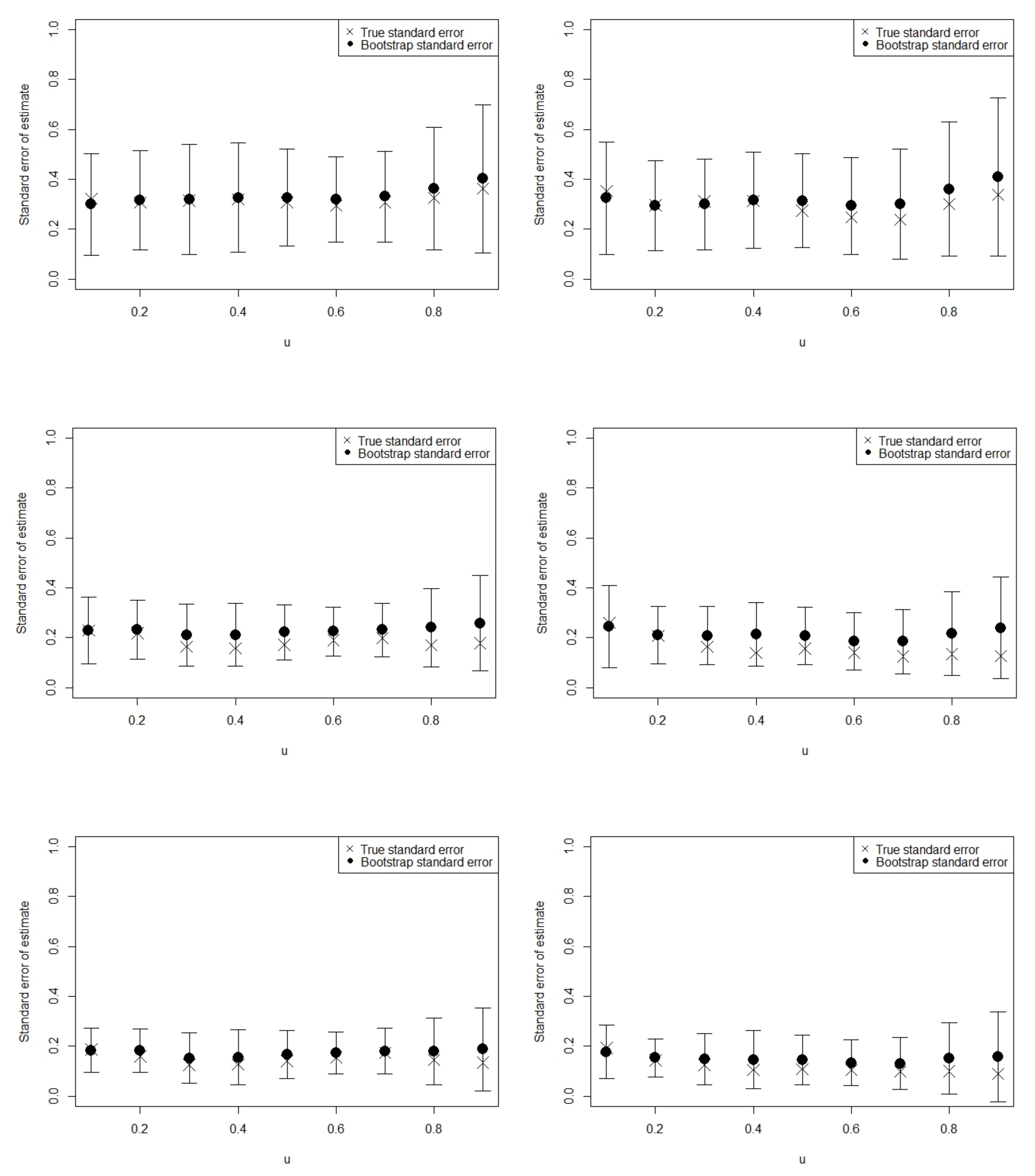
Standard Errors and Confidence Intervals

We use the bootstrap approach to approximate the point-wise standard errors of the estimates as well as the confidence intervals for the model parameter functions. For a given $x_0$ we use the estimated model to generate the corresponding $y^{*}\sim {\sum }_{k=1}^K\widehat{\pi }\left(x_0\right)\mathcal{N}\{{\widehat{m}}_k\left(x_0\right),{\widehat{\sigma }}_k^2\left(x_0\right)\}$; this way we generate the bootstrap sample denoted by $\{(x_i,y_i^{*}):i=1,2,\dots ,n\}$. We generate $B=1000$ such samples to produce bootstrap fitted models to approximate the point-wise standard errors and confidence intervals.

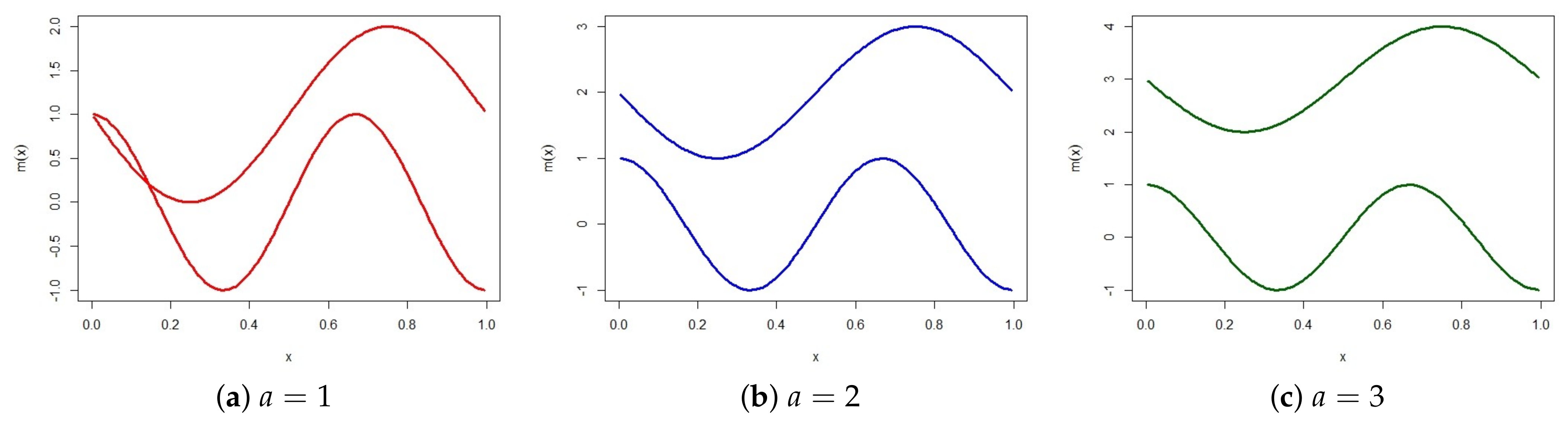
3.4. Simulation Studies

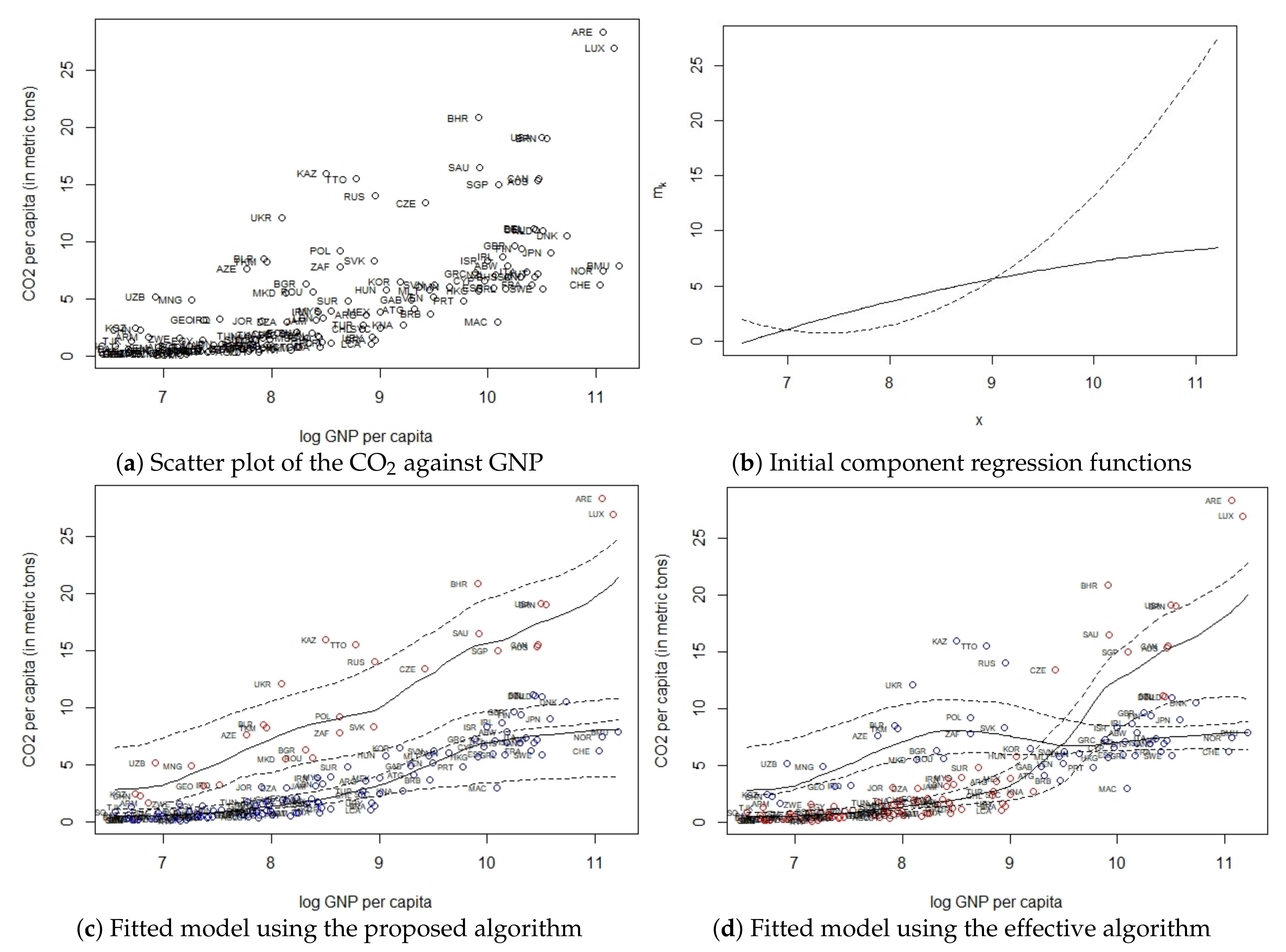
In this section, we perform a simulation study on artificial data to demonstrate the performance of the proposed algorithm (Algorithm 2). We will compare our proposed method with the effective algorithm of Huang et al. [8]. For this simulation, we generate the data from the two-component NPGMRs model given in Table 1.

Table 1. NPGMRs model generating the data.

Functions	Component (k)
	1	2
${\pi }_k\left(x\right)$	$exp\left(0.5x\right)/\{1+exp(0.5x\left)\right\}$	$1-{\pi }_1\left(x\right)$
$m_k\left(x\right)$	$a-sin\left(2\pi x\right)$	$cos\left(3\pi x\right)$
${\sigma }_k(x$)	$0.6exp\left(0.5x\right)$	$0.5exp(-0.2x)$

The covariate $x\sim Uniform(0,1)$, where $Uniform(\alpha ,\beta )$ denotes a uniform distribution with parameters $\alpha$ and $\beta$. The constant a controls the degree of separation between the components, ranging from $a=1$ poorly separated to $a=3$ well separated components. The different scenarios are shown in Figure 2. We will generate 500 samples of sizes $n=200$, 400 and 800 and take a 100 grid points chosen evenly from the support of the covariate x. The simulation results are given in Table 2. The table gives the average and standard deviation of two of the performance measures over the 500 simulations. We can see from the table that when a is small, proposed algorithm gives better results and as the components become more separated, that is as a increases, the performance of the proposed algorithm and the effective algorithm is similar. The rest of the performance measures (not given) lead to the same observation. This shows that the proposed algorithm is most effective when the components are not well separated. This might be due to the difficulty of choosing an appropriate initial state when the components are not well separated. Moreover, this is likely to be a challenge for the effective algorithm since for this algorithm the E-step estimates (global responsibilities) are more dependent on the initial state compared to the proposed algorithm. This is because the latter uses all the local responsibilities from the E-step; it is thus less sensitive to its initial state. This is largely due to the possible mismatch in the component labels at each grid point which may allow the global responsibilities and ultimately the non-parametric estimates to be independent of its the initial state. This highlights the advantage of taking into account the local responsibilities to obtain the global responsibilities. We demonstrate this phenomena through simulation, where the algorithms are initialized at an inferior state. We use the same sampling setting as above, with $a=2$ and $n=400$. We record the average and standard deviation of RASE${}_m$ and number of times the algorithm couldn’t escape the initial state, denoted as $ntrap$. Table 3 gives the results. All 500 simulations were initialized from the model with the component regression functions given as in Figure 3 and the other two functions initialized at their true functions. As can be seen from the table, the effective algorithm was trapped at its initial state 325 times out of 500, whereas the proposed algorithm was trapped only once.

Figure 2. Plots of the component regression functions for the three scenarios of the two-component NPGMRs model.

Table 2. Average (and standard deviation) of the performance measures for 500 samples.

	Scenario
	a = 1		a = 2		a = 3
	RASEm	R2	RASEm	R2	RASEm	R2
$n=200$
Proposed Algorithm	0.3604 (0.0849)	69.7196 (5.0879)	0.2546 (0.0683)	77.7391 (3.6825)	0.2026 (0.043)	86.2399 (2.0393)
Effective Algorithm	0.4339 (0.1374)	68.7144 (5.4797)	0.299 (0.1723)	77.3533 (4.0877)	0.2122 (0.0743)	86.2229 (2.1173)
$n=400$
Proposed Algorithm	0.3018 (0.0678)	69.1957 (3.7468)	0.1929 (0.0427)	77.7333 (2.6144)	0.1545 (0.0296)	86.3577 (1.2879)
Effective Algorithm	0.3987 (0.1359)	67.7125 (4.0693)	0.2132 (0.0696)	77.3875 (2.7089)	0.157 (0.0396)	86.3374 (1.3074)
$n=800$
Proposed Algorithm	0.2533 (0.0494)	68.9866 (2.7873)	0.1485 (0.0278)	77.8396 (1.9831)	0.059 (0.0119)	86.3538 (0.9668)
Effective Algorithm	0.3905 (0.1502)	67.3622 (3.3621)	0.1671 (0.0439)	77.5533 (2.0859)	0.1197 (0.0305)	86.3476 (0.9778)

Table 3. Evaluating the sensitivity of the proposed algorithm to its initial state.

Algorithm	RASE${}_{\mathit{m}}$	$\mathit{ntrap}$
Proposed Algorithm	0.1944 (0.0445)	1
Effective Algorithm	0.2539 (0.0715)	325

Figure 3. Initial component regression functions.

Next, we demonstrate the performance of the bootstrap procedure for calculating the standard errors of the estimates. This demonstration is based on the scenario with $a=2$, the results are shown in Figure 4 only for the component mean functions for different sample sizes. The grid points $u=0.1,0.2,\dots ,0.9$ were used. The plots give the point-wise standard deviations of the estimates over 500 samples which represents the true standard errors (SD) at the grid points, as labelled on the graph. The results show slight over- and under-estimations; however, the procedure works well as it shows that the SD are within two standard errors of the estimated point-wise bootstrap standard errors (SE). This can be observed on the plot which shows that all the SDs are within the error bars, the latter were calculated as the approximate 95% point-wise bootstrap confidence intervals. The bootstrap procedure works similarly for both the variance and mixing proportion functions.

Figure 4. Bootstrap standard errors: plots of the estimated point-wise bootstrap standard errors at the grid points (shown by the bullet) for the estimated mean function of component 1 (left panel) and component 2 (right panel) for sample sizes $n=200$ (top panel), $n=400$ (middle panel) and $n=800$ (bottom panel). The error bars represent the approximate 95% point-wise bootstrap confidence intervals at the grid points. We also plot the point-wise standard errors (shown by the cross) obtained as the standard deviation of 500 estimates at the grid points.

4. Application

In this section, we demonstrate the usefulness of our proposed algorithm on real data.

4.1. Problem and Data Description

The data consist of the per capita CO${}_2$ emissions (in metric tons) and the per capita GNP (in US$) (on a log base e scale) for a sample of 145 countries for the year 1992. For a given country, the first measure gives the estimated amount of CO${}_2$ emitted by each resident during the year, whereas the second measure gives the total value of goods and services produced by each resident. The data were extracted from the World Development Indicators database of the World Bank Group. The data are plotted in Figure 5a. Each data point on the figure is labelled by the corresponding country’s code, for example ZAF is South Africa and CZE is Cezch Republic. Hurn et al. [7] had a similar dataset for the year 1996 and they identified a two-component mixture regression structure consisting of two groups of countries. They further mentioned that the identification of these groups “…may help to clarify on which development path they are embarking”. They fitted a GMLRs model on their dataset.

Figure 5. Application data and fitted NPGMRs model: (a) scatter plot of the data, (b) initial component regression functions, (c) fitted $K=2$ component NPGMRs model using proposed algorithm and (d) using the algorithm in Huang et al. The dotted curves give the point-wise 95% bootstrap confidence intervals obtained using 5000 bootstrap samples.

4.2. Modelling and Results

We fit the NPGMRs to the data set plotted in Figure 5a and identify the best model for $K=1,2,\dots ,5$ being the model that minimises the BIC. We also fit the GMLRs model. We use the procedure outlined above (Section 3.1) to choose the bandwidth for each K. The resulting BIC values are presented in Table 4 and we can clearly see that the BIC favours a two-component ($K=2$) NPGMRs model. Figure 5c plots the estimated model. The components were identified by hard classification. We can see from the figure that, for the year 1992, for one group of countries (shown in red points), which includes the United Arab Emirates (ARE), a higher income per capita corresponded with a higher quantity of CO${}_2$ emitted per capita. On the other hand, for the other group of countries (shown in blue), which includes Switzerland (CHE), a higher income per capita corresponded with a lower quantity of CO${}_2$ emitted per capita. Furthermore, for the latter group of countries, the increase in CO${}_2$ per capita seems to have reached a peak as it plateaus beyond an income per capita of about US$ 22,027 (given by $e^{10}$).

Table 4. BIC values for mixture regression models fitted on the climate data.

Model	K	h	BIC
NPGMRs	1	0.95	770.7226
	$\mathbf{2}$	$\mathbf{0}.\mathbf{945}$	$\mathbf{706}.\mathbf{9895}$
	3	0.945	766.3612
	4	0.95	819.9092
	5	0.9	916.5939
GMLRs	1		810.1633
	1		811.2591
	2		760.8051
	3		754.7527
	4		788.4389

The fitted model was compared with the model obtained with the effective algorithm of Huang et al. The fitted model using the latter algorithm is given in Figure 5d. Notice that the fitted model has a different interpretation of the data but the model based on the proposed algorithm is the best model as seen from Table 5. A closer look at the fitted component regression functions in Figure 5d reveals that the fitted functions have the same form as the component regression functions used to initialize the algorithm, see Figure 5b. This is a further indication of the effective algorithm’s initial state dependence. We tried to improve on the initial state by instead running each pth-degree polynomial for 100 times but we obtained the same initial state.

Table 5. Performance measures for the fitted $K=2$ component NPGMLRs model.

Algorithm	Performance Measures
	BIC	R${}^2$
		Estimated	Bootstrap Mean (Std)	95% (Lower) Bootstrap	95% (Upper) Bootstrap
Proposed Algorithm	$\mathbf{706}.\mathbf{9895}$	83.3556	80.7076 (6.1293)	63.8578	89.1703
Effective Algorithm	718.4571	73.8182	70.0673 (5.8218)	57.9395	80.5303

Important to point out though is that both fitted models are in agreement with the environmental Kuznets curve (EKC) hypothesis [20]. The hypothesis states that, as a country becomes industrialized, its carbon emissions increase faster than its income. This environmental degradation continues up until a certain level of income. Beyond this level of income, there is a reduction in carbon emissions. Thus, the EKC hypothesis postulates an inverted-U shaped relationship between environmental degradation (such as carbon emissions) and income. Assuming that all countries follow the same EKC then, at any time for a cross section of countries representing different income groups, it should be observed that poor countries are yet to be industrialized and thus are at the initial stage of the EKC, some developing countries are in the process of industrialisation and thus are at or approaching the peak emission levels and finally developed countries are beyond the peak. Evidence of this is easily seen in Figure 5. For one group of countries (shown in blue points), which includes a lot of high income countries, the peak emission level is reached, whereas for the other group (shown in red points), which has mainly low–middle income countries, by 1992 standards, a peak is yet to be reached.

We evaluate the normality of the component error distributions using the Kolmogorov–Smirnov (KS) goodness-of-fit test. For each component, we calculate the residuals as ${\widehat{\gamma }}_{ik}[y_i-\widehat{m}\left(x_i\right)]{\mathbb{I}}_{[{\widehat{\gamma }}_{ik}>0.5]}$, for $k=1,2,\dots ,K$, where ${\mathbb{I}}_{[·]}$ is an indicator function taking a value of 1 when ${\widehat{\gamma }}_{ik}>0.5$ and 0 otherwise. Table 6 gives the results of the KS test of normality of the two fitted component distributions based on the proposed algorithm and the effective algorithm. The calculations were conducted using the ks.test function from the stats package of the R programming language [21]. The normality of each of the two components fitted by the proposed algorithm cannot be rejected. The normality of the first component fitted by the effective algorithm is rejected and that of the second component cannot be rejected at a 5% significance level.

Table 6. Kolmogorov–Sminorv (KS) test of normality of the two fitted component distributions.

Algorithm	Component 1		Component 2
	Test Statistic	p-Value	Test Statistic	p-Value
Proposed Algorithm	0.1622	0.3690	0.1069	0.1441
Effective Algorithm	0.2589	<0.0001	0.1733	0.0690

5. Discussion

In this paper, we propose an EM-type algorithm to simultaneously maximize the local-likelihood functions (LLFs) when estimating the non-parametric functions of an NPGMRs model. The performance of the proposed algorithm is demonstrated using a simulation study and a real data problem. For illustrative purposes, our simulation study considered only two-component NPGMRs models although the algorithm can be applied for any number of mixture components. To see how the proposed algorithm performs for poorly separated mixture regression components, the results show a declining estimation error as we increase the sample size, empirically demonstrating consistency. A comparison of the proposed algorithm with a competitive algorithm reveals some interesting points: (1) for poorly separated mixture components, the proposed algorithm shows a better performance, whereas for well separated components the performance of the two algorithms is similar; (2) the proposed algorithm is independent of its initial state. This is demonstrated by initializing both algorithms at the same inferior state and 100% of the time the proposed algorithm escaped the initial state, whereas the competitive algorithm only managed to escape only 35% of the time. The first point implies that our algorithm is more effective at identifying the true mixture structure for complex mixture structures relative to the competitive procedure. The second point implies that, for the proposed algorithm, not much consideration should be given to the optimal choice of the initial state.

For our real data example, we considered the relationship between CO₂ emissions (as the response) and national income (as a covariate) for a group of 145 countries. The effectiveness of the proposed algorithm was demonstrated by its ability to identify two latent components wholly independent of the initial conditions. Using a goodness-of-fit test, we showed that the Gaussian assumption on the component distributions of the two fitted components, based on the proposed algorithm, is appropriate.

6. Conclusions

This paper presents a novel a EM-type algorithm to simultaneously maximize the local likelihood functions (LLFs) when estimating the NPGMRs model. This proposal is made in response to a potential mismatch in the responsibilities obtained at the E-step when the LLFs are maximized separately. The result is wiggly and less smooth estimated non-parametric functions as shown in Figure 1c giving rise to a component label switch, hence the label-switching problem. Less sensitivity to label switching can be achieved by making sure that the responsibilities match at each local point. Thus, a global estimate of the responsibilities must be obtained. The proposed algorithm takes as its estimated global responsibilities, the local responsibilities that result in the smoothest estimated component functions. The performance of the proposed algorithm is demonstrated using a simulation study and a real data problem.

Although the proposed approach has some practical advantage (less sensitivity to its initial state), it is unable to identify the true structure of more complex (overlapping or intersecting component functions) mixture structures (an example of a complex mixture structure can be obtained for $0<a<1$ in our simulations). This is possibly due to the discrete nature of our approach in the sense that one of the local responsibilities are chosen as the global responsibilities. This in turn results in loss of information.

Thus, future research should explore the prospects of a continuous version of the proposed algorithm. Perhaps some form of a probabilistic combination of the local responsibilities can prevail over this challenge.

References

- Titterington, D.M.; Smith, A.F.M.; Makov, U.E. Statistical Analysis of Finite Mixture Distributions; John Wiley and Sons: Hoboken, NJ, USA, 1985. [Google Scholar]
- Frühwirth-Schnatter, S.; Celeux, G.; Robert, C.P. Handbook of Mixture Analysis; Chapman and Hall/CRC: Boca Raton, FL, USA, 2019. [Google Scholar]
- Quandt, R.E. A New Approach to Estimating Switching Regressions. J. Am. Stat. Assoc. 1972, 67, 306–310. [Google Scholar] [CrossRef]
- Goldfeld, S.M.; Quandt, R.E. A Markov model for switching regressions. J. Econom. 1973, 1, 3–15. [Google Scholar] [CrossRef]
- Quandt, R.E.; Ramsey, J.B. Estimating Mixtures of Normal Distributions and Switching Regressions. J. Am. Stat. Assoc. 1978, 73, 730–738. [Google Scholar] [CrossRef]
- Frühwirth-Schnatter, S. Finite Mixture and Markov Switching Models; Springer Science & Business Media: New York, NY, USA, 2006. [Google Scholar]
- Hurn, M.; Justel, A.; Robert, C.P. Estimating mixtures of regressions. J. Comput. Graph. Stat. 2003, 12, 55–79. [Google Scholar] [CrossRef]
- Huang, M.; Li, R.; Wang, S. Nonparametric mixture of regression models. J. Am. Stat. Assoc. 2013, 108, 929–941. [Google Scholar] [CrossRef] [PubMed] [Green Version]
- Xiang, S.; Yao, W. Semi-parametric mixtures of non-parametric regressions. Ann. Inst. Stat. Math. 2018, 70, 131–154. [Google Scholar] [CrossRef]
- Wu, X.; Liu, T. Estimation and testing for semiparametric mixtures of partially linear models. Commun. Stat.-Theory Methods 2017, 46, 8690–8705. [Google Scholar] [CrossRef]
- Zhang, Y.; Zheng, Q. Semiparametric mixture of additive regression models. Commun. Stat.-Theory Methods 2018, 47, 681–697. [Google Scholar] [CrossRef]
- Zhang, Y.; Pan, W. Estimation and inference for mixture of partially linear additive models. Commun.-Stat.-Theory Methods 2020, 51, 2519–2533. [Google Scholar] [CrossRef]
- Xiang, S.; Yao, W. Semi-parametric mixtures of regressions with single-index for model based clustering. Adv. Data Anal. Classif. 2020, 14, 261–292. [Google Scholar] [CrossRef] [Green Version]
- Xiang, S.; Yao, W.; Yang, G. An Overview of Semi-parametric Extensions of Finite Mixture Models. Stat. Sci. 2019, 34, 391–404. [Google Scholar] [CrossRef] [Green Version]
- Tibshirani, R.; Hastie, T. Local likelihood estimation. J. Am. Stat. Assoc. 1987, 82, 559–567. [Google Scholar] [CrossRef]
- Dempster, A.P.; Laird, N.M.; Rubin, D.B. Maximum likelihood from incomplete data via the EM algorithm. J. R. Stat. Soc. Ser. B Methodol. 1977, 39, 1–38. [Google Scholar]
- Stephens, M. Dealing with label switching in mixture models. J. R. Stat. Soc. Ser. B Stat. Methodol. 2000, 62, 795–809. [Google Scholar] [CrossRef]
- Tibshirani, R.; Walther, G. Cluster validation by prediction strength. J. Comput. Graph. Stat. 2005, 14, 511–528. [Google Scholar] [CrossRef]
- Ingrassia, S.; Punzo, A. Cluster validation for mixtures of regressions via the total sum of squares decomposition. J. Classif. 2020, 37, 526–547. [Google Scholar] [CrossRef]
- Dinda, S. Environmental Kuznets curve hypothesis: A survey. Ecol. Econ. 2004, 49, 431–455. [Google Scholar] [CrossRef] [Green Version]
- R Core Team. R: A Language and Environment for Statistical Computing; R Foundation for Statistical Computing: Vienna, Austria, 2022. [Google Scholar]
Publisher’s Note: MDPI stays neutral with regard to jurisdictional claims in published maps and institutional affiliations. |
© 2022 by the authors. Licensee MDPI, Basel, Switzerland. This article is an open access article distributed under the terms and conditions of the Creative Commons Attribution (CC BY) license (https://creativecommons.org/licenses/by/4.0/).