Exploiting Asymmetric EEG Signals with EFD in Deep Learning Domain for Robust BCI

Abstract

Motor imagery (MI) is a domineering paradigm in brain–computer interface (BCI) composition, personifying the imaginary limb motion into digital commandments for neural rehabilitation and automation exertions, while many researchers fathomed myriad solutions for asymmetric MI EEG signals classification, the existence of a robust, non-complex, and subject-invariant system is far-reaching. Thereupon, we put forward an MI EEG segregation pipeline in the deep-learning domain in an effort to curtail the existing limitations. Our method amalgamates multiscale principal component analysis (MSPCA), a novel empirical Fourier decomposition (EFD) signal resolution method with Hilbert transform (HT), followed by four pre-trained convolutional neural networks for automatic feature estimation and segregation. The conceived architecture is validated upon three binary class datasets: IVa, IVb from BCI Competition III, GigaDB from the GigaScience repository, and one tertiary class dataset V from BCI competition III. The average 10-fold outcomes capitulate 98.63%, 96.33%, and 89.96%, the highest classification accuracy for the aforesaid datasets accordingly using the AlexNet CNN model in a subject-dependent context, while in subject-independent cases, the highest success score was 97.69%, outperforming the contemporary studies by a fair margin. Further experiments such as the resolution scale of EFD, comparison with other signal decomposition (SD) methods, deep feature extraction, and classification with machine learning methods also accredits the supremacy of our proposed EEG signal processing pipeline. The overall findings imply that pre-trained models are reliable in identifying EEG signals due to their capacity to maintain the time-frequency structure of EEG signals, non-complex architecture, and their potential for robust classification performance.

1. Introduction

1.1. What Is BCI?

A brain–computer interface (BCI) is a long-standing research dominion that enables a direct communication channel between the brain and the computer. The term BCI refers to a system that works in tandem with the brain to allow for the control of external activities like moving a cursor or operating a prosthetic limb through the use of brain signals. The interface establishes a line of neural communication between the brain and the controlled object. For example, instead of the signal traveling through the neuromuscular system from the brain to the finger on a mouse, it is sent directly from the brain to the mechanism controlling the cursor. A BCI can help a paralyzed person write a book or operate a powered wheelchair or prosthetic limb with only their thoughts by reading signals from an array of neurons and translating the signals into action using computer chips and programming. Some future applications, like prosthetic control, are likely to function automatically, but the current generation of brain-interface devices needs conscious, intentional thought. Creating non-invasive electrode devices and/or surgical techniques has been a significant hurdle in the advancement of BCI technology. In the conventional BCI concept, an implanted mechanical device is integrated into the patient’s mental image of their body, and the patient exercises control over the device as if it were an extension of their own body. Non-invasive brain–computer interfaces (BCIs) are currently the subject of extensive study.

Decades of study in BCI have yielded several novel hypotheses and frameworks with wide-ranging implications in neurological rehabilitation, prosthetics, robotics, augmented reality, and assistive technologies [1]. The elementary bedrock of BCI is a fragile electroencephalogram (EEG) signal over the cranial dermis, spawned proportionately to excitatory or inhibitory cerebral activity, while EEG is a non-invasive mode of procuring signals, it dominates its compeers, i.e., electrocorticography (ECoT), magnetoencephalography (MEG), magnetic resonance imaging (MRI), functional magnetic resonance imaging (fMRI), and positron emission tomography (PET), in several aspects such as low cost and portable equipment, high temporal resolution, ease of setup and safe to use nature [2].

1.2. BCI Paradigms

Owing to their operational characteristics, BCI EEG is classified into three major paradigms, namely, motor imagery (MI), event-related potential (ERP), and steady-state visually evoked potential (SSVEP) [3]. The MI is a self-regulated cognitive endeavor where a subject mentally rehearses a limb motion without literally performing that motion in actual, giving rise to an active BCI. The ERP and SSVEP, on the other hand, make up a reactive BCI architecture that requires an external stimulus to function. The task segregation in MI necessitates robust identification of the changes in $\mu$ (8–13Hz) and $\beta$ (13–30Hz) bands called event-related synchronization/ desynchronization (ERS/ERD) [4]. As a result of such non-stationary spectral variations, MI EEG undergoes laborious signal processing procedures in an effort to translate the time-varying signals into actionable commands. Consequently, the present study aims to formulate a signal-processing pipeline that could serve as a stalwart basis for MI EEG identification.

1.3. Literature Review

The MI EEG signal processing entails a series of steps: data preparation, non-stationary to stationary data transformation, feature extraction, and classification. Initially, the scalp-recorded EEG signals are densely contaminated by noise artifacts such as power line interference, ambient noise, ocular noise, electrocardiogram (ECG), electromyogram (EMG), etc. Such alienated samples make it harder to separate EEG tasks, so they need to be filtered out before the signal is further processed. In the literature, the commonly employed data filtering methods incorporate Bayes filters [5], Weiner filters [6], recursive least square (RLS) strategy [7], principal component analysis (PCA) [8], independent component analysis (ICA) [9], and sparse component analysis (SPA) [10]. However, these approaches have certain drawbacks in their applicability, such as they do not take inter-channel correlated characteristics into account, they have strong parametric dependencies which makes them hard to use for a practical BCI system, they often require a reference signal to denoise the EEG data, and they are sensitive to outliers. Recently, biological signals have made extensive use of a hybrid dimensionality reduction method called multiscale principal component analysis (MSPCA) [11]. Scientific investigation [12] shows that MSPCA overcomes the shortcomings of traditional filtering techniques and achieves promising classification performance at low signal-to-noise ratios (SNRs).

The next step in EEG data processing is to resolve non-stationary signals into stationary sub-bands. Signal decomposition (SD) is efficacious for the time-frequency analysis of MI EEG signals since the task-specific information occurs within the $\mu$ and $\beta$ bands. For this purpose, the contemporary studies exploited empirical mode decomposition (EMD) [13], ensemble empirical mode decomposition (EEMD) [14], variational mode decomposition (VMD) [15], wavelet transform, empirical wavelet transform (EWT) [16], wavelet packet decomposition (WPD) [17], and tunable-Q wavelet transform (TQWT) [18], while each of these techniques has its uses, they also have its share of downsides, such as the mixing of modes, tight spacing of frequencies, selection of mother wavelets, lack of organized frequency bands, susceptibility to noise, computationally laborious, etc. To mitigate the afore-stated challenges with traditional SD methods, our previous study contemplated a hybrid empirical Fourier decomposition (EFD) method [19]. The proposed method resolved the non-stationary EEG into a pre-defined number of intrinsic mode functions (IMFs) without any parametric contingence and addressed the prevailing shortcomings.

Following SD, the time-frequency EEG signals are condensed into a set of meaningful scalar values called features. The robust classification of MI EEG relies heavily upon the type and number of extracted features. The commonly employed attribute acquisition methods in the EEG domain involve energy and entropy features [20], fractal dimensions [21], time and statistical features [22], spectral features [19], matrix determinant [12], successive decomposition index (SDI) [23], common spatial patterns (CSPs) [24], and graphical features [22]. Such attributes are handcrafted and manually engineered by numerous research studies, and their classification performance is somewhat satisfactory, yet they possess several drawbacks such as noise sensitivity, susceptibility to the input data, ineptness for a large number of data samples, loss of time/frequency resolution, etc. Recently, the idea of extracting automatic features from deep convolutional neural networks (CNNs) has been gaining immense attention [25]. Deep features are iteratively learned from the input data while the CNN is being trained. Some standard references for deep feature extraction are AlexNet [26], GooglNet [26], ShuffleNet [27], deep ConvNet [28], EEGNet [29], 1D-ConvNet [30], etc.

1.4. Objectives and Contributions

In order to address the shortcomings with those SDs, feature extraction and classification methods, this research synthesizes a new classification pipeline for MI EEG signals using our previously proposed empirical Fourier decomposition (EFD) [19] in conjunction with pre-trained convolutional neural network (CNN) modules. The proposed mechanism, called EFD-CNN, operates under the coexistence of four distinct signal-processing modules. First, the MI EEG data is preprocessed for artifact removal employing the MSPCA method. Second, the EFD method is adopted to decompose the non-stationary, non-linear and asymmetric EEG signals into several bandlimited subcomponents. Third, the decomposed components are converted into time-frequency scalograms employing the Hilbert transform (HT). Fourth, the 2D time-frequency-amplitude scalograms are fed to four pre-trained CNN models, namely AlexNet, ShuffleNet, GoogleNet, and SqueezeNet, for automatic feature extraction and classification. The main contributions of this study are as follows:

• To alleviate the high complexity, extensive computational load, as well as large fluctuation caused by manual feature extraction [19,31], the EFD combined with pre-train CNN models is proposed to contrive a non-complex and automatic feature extraction model. To the best of our knowledge and understanding, this study is the first attempt to combine EFD with any kind of CNN model and estimate its utility for MI EEG problems.
• To accredit the performance invariance for changing datasets, the proposed EFD-CNN design is validated upon four large- and small-scale binary and tertiary-class MI EEG datasets. The deployed datasets incorporate binary class datasets IVa and IVb from BCI competition III containing six subjects altogether, a binary class GigaDB dataset from the GigaScience repository containing EEG data from 52 participants, and a three-class dataset V from BCI competition III having three subjects collectively.
• A subject-independent framework is exploited by training the EFD-CNN model over the data from a particular group of subjects while testing it over an unseen subject. This is particularly interesting for a real-time BCI system since it allows the subject-to-subject transfer of learned model parameters and the reusability of the current model for a large group of new users.
• An extensive quantitative analysis, including an assessment of 10-fold classification performance, the effect of a varying number of EFD modes, deep feature extraction from CNN models and classification with machine learning models, and comparison with contemporary studies, are performed and validated.

The remaining sections of this article are structured as follows. In Section 2, we talk about the datasets used in this study. In Section 3, the readers can find a list of methods and detailed descriptions used in this framework. Section 4 narrates the experimental arrangements. Section 5 describes and discusses the empirical outcomes for different case scenarios. Section 6 marks the prospects and limitations of the current study. Lastly, Section 7 concludes this study.

2. Offline Data Repositories

This study exercises four large- and small-scale EEG datasets containing binary and tertiary MI tasks for EFD-CNN validation. Such data cohorts include binary class MI EEG dataset IVa, IVb from BCI competition III [32], GigaDB dataset from GigaScience repository [3], and a three-class dataset V from BCI competition III [32]. The essential characteristics and acquisition protocols of all repositories are illustrated in Table 1, while a brief description concerning each dataset is as follows:

Table 1. List of the MI EEG data repositories utilized in this study.

Dataset #	Dataset Name	Sampling Rate	Trial Duration (s)	No. of Electrodes	Participants	Class 1 Trials	Class 2 Trails	Class 3 Trails
Dataset 1	IVa from BCI Competition III [32]	100	35	118	A1 = AA	80	86	-
					A2 = AL	112	112
					A3 = AV	42	42
					A4 = AW	30	26
					A5 = AY	18	10
Dataset 2	IVb from BCI Competition III [32]	100	3.5	118	B	105	105	-
Dataset 3	GigaDB from GigaScience [3]	512	3	64	S1–S52	100 or 120	100 or 120	-
Dataset 4	V from BCI Competition III [32]	512	1	32	Subject 1	280	200	236
					Subject 2	276	201	237
					Subject 3	238	235	238

• $\mathit{Dataset}\mathbf{1}$: Dataset IVa includes two MI EEG tasks for the right hand (RH, class 1) and right foot (RF, class 2). The computer-aided visual system cued five healthy individuals named AA (A1), AL (A2), AV (A3), AW (A4), and AY (A5) for 3.5 s per task and captured data at 1000 Hz in 118 channels using the International 10-20 system. Each individual completed 280 experiments, including 140 trials for the right hand and 140 samples for the right foot category.
• $\mathit{Dataset}\mathbf{2}$: Dataset IVb is a single-subject EEG dataset with MI tasks for the left hand (LH, class 1) and right foot (RF, class 2). Similar to dataset 1, dataset 2 provides the subject (annotated as subject B) with a 3.5 s visual cue and records data at 1000 Hz with 118 channels. A total of 210 trials were carried out, half with class 1 tasks and the other half with class 2 tasks. Datasets 1 and 2 are downscaled to 100 Hz and filtered with a bandpass filter ranging from 0.5 to 200 Hz.
• $\mathit{Dataset}\mathbf{3}$: GigaDB is a binary class MI EEG signals database collected from 52 participants (including 33 male and 19 female subjects). The information was gathered using 64 Ag/AgCl electrodes in accordance with the International 10-10 standard. Each MI task consisted of 100 or 120 trials lasting for 3 s at a sampling rate of 512 Hz.
• $\mathit{Dataset}\mathbf{4}$: Dataset V has three MI EEG tasks, including imagining repetitive self-paced left-hand movements (class 1), imagining repetitive self-paced right-hand movements (class 2), and generating words starting with random letters (class 3). Three subjects participated in extensive trials for different MI tasks, each last for one second while the data was sampled at 512 Hz using 32 electrodes.

3. Method

3.1. Step 1: Denoising with Multiscale Principal Component Analysis

The EEG signals accumulation process is densely fabricated by noise artifacts originating as a result of biological activities such as the electrocardiogram (ECG), electrooculogram (EOG), electromyogram (EMG), systematic noise coming from within the EEG gauging equipment, power line interference, and communication systems artifacts. The foremost operation is to identify and filter out such alienated superpositions in order to acquire clean signals populated with MI EEG task-specific information. We opt for a hybrid denoising tool called multiscale principal component analysis (MSPCA) for MI EEG filtration to attain the desired objective. The MSPCA combines principal component analysis (PCA) and wavelet transform (WT) to sift out the noisy samples from the actual data using their covariance property and repack the remaining data to output a denoised multichannel EEG signal. The block diagram for MSPCA workflow is given in Figure 1, while a brief working principal is narrated as follows:

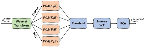
Figure 1. MSCPA workflow illustration.

• Let m be the number of time samples in an EEG signal, and n be the number of channels. The single-trial EEG signal matrix could be defined as $A_{m\times n}$.
• Fragment each channel of matrix A into Q levels using wavelet transform to obtain $B_i$B (detailed coefficients) and $A_j$B (approximate coefficients).
• Normalize the wavelet coefficients at each scale and conduct the principal component analysis (PCA). As per Kaiser’s criterion, choose the coefficients with eigenvalues greater than the average of all eigenvalues.
• Calculate the inverse wavelet transform of the selected coefficients.
• Calculate the PCA of the resultant matrix to obtain the denoised EEG signals.

The MSPCA was first introduced in [33] as a dimensionality reduction tool, but its efficiency for biological signals has been demonstrated in recent research [12,23]. In this investigation, we used Symlets 5 mother-wavelet for WT and set the wavelet decomposition level (Q) to five. Such parameter setting is based on best practices used in earlier studies, and the empirical hit and trial analysis in this study also attests to best-case outcomes for the aforementioned parameter choices.

3.2. Step 2: Signal Resolution with Empirical Fourier Decomposition

The foundation of empirical mode decomposition (EFD) derives characteristics from the Fourier decomposition method (FDM) in terms of resolving a signal using Fourier intrinsic band functions (FIBFs) and empirical wavelet transform (EWT) for boundary detection in a Fourier spectrum. When contrasted to EWT, EFD workflow is concise and does not necessitate any transformation or mother wavelet selection. To begin with, the segmentation of the Fourier spectrum and detection of boundaries is the first critical step in calculating the EFD of a non-stationary and non-linear signal. The user specifies M decomposition levels for a given Fourier spectrum (spanning from 0 to $\pi$), and M + 1 boundaries are ultimately required. The Q critical points (starting point and local minima) in the spectrum are then identified and sorted in descending order. Next, the appropriate number of critical points are stipulated considering the following two conditions:

• If N ≥ M, where N is the maximum number of pivot points in a Fourier spectrum, the first M − 1 points are chosen.
• If N < M, the number of extractable modes is less than the desired decomposition level, and hence M is automatically reset to N.

Subsequently, the position (${\Omega }^q$) of such critical points is estimated provided that 1 ≤ m ≤ M − 1, ${\Omega }^0$ = 0, and ${\Omega }^m$ = $\pi$. Lastly, the absolute minimum in the range [${\Omega }^{m-1}$, ${\Omega }^m$] is designated as border point ${\Omega }^m$, and the set of minima is symbolized as ${\omega }_m$. The entire Fourier spectrum boundaries could be defined as:

$${\Omega }_q=\left\{\begin{array}{c}argmin{\omega }_q,for1⩽m⩽M-1\hfill \\ \frac{{\Omega }^{M-1}+{\Omega }^M}{2},form⩽M\hfill \end{array}\right.$$

(1)

The next step is to calculate the IMFs once the Fourier spectrum limits have been found. Consider a real-valued, time-limited EEG signal z(t), which has the following Fourier series expansion:

$$\left\{\begin{array}{c}\begin{array}{c}{c}_0=\frac{2}{Q}{\int }_{t_2}^{t_1+Q}z\left(t\right)dt\hfill \\ c_m=\frac{2}{Q}{\int }_{t_2}^{t_1+Q}cos\left(q{\varphi }_{0}t\right)z\left(t\right)dt\hfill \\ d_m=\frac{2}{Q}{\int }_{t_1}^{t_1+Q}sin\left(q{\varphi }_{0}t\right)z\left(t\right)dt\hfill \\ z\left(t\right)=\frac{c_0}{2}+\sum _{q=1}^{\infty }\left[c_{q}cos\left(q{\varphi }_{0}t\right)+d_{q}sin\left(q{\varphi }_{0}t\right)\right]\hfill \end{array}\hfill \end{array}\right.$$

(2)

where c and d denote the Fourier series coefficients. It is possible to express Fourier series expansion in its Euler form as follows:

$$z\left(t\right)=\frac{c_0}{2}+\frac{1}{2}\sum _{q=1}^{\infty }\left[y_q{e}^{\left(jq{\varphi }_{0}t\right)}+y_q^{*}{e}^{\left(-jq{\varphi }_{0}t\right)}\right]$$

(3)

where $y_q$ = ($c_q$−$j{d}_q$ )and $y_q^{*}$ = ($c_q+j{d}_q$). The analytic expression for FIBF could be described as follows:

$$\left\{\begin{array}{c}w\left(t\right)=\sum _{q=1}^{\infty }{y}_q{e}^{\left(jq{\varphi }_{0}t\right)}\hfill \\ \stackrel{-}{w}\left(t\right)=\sum _{q=1}^{\infty }{y}_q^{*}{e}^{\left(-jq{\varphi }_{0}t\right)}\hfill \end{array}\right.$$

(4)

Hereby, Equation (3) can be transformed as:

$$z\left(t\right)=\frac{c_0}{2}+\mathrm{Re}\left\{w\left(t\right)\right\}$$

(5)

The previously specified segmentation criteria indicate that w(t) may be divided into M − 1 segments, and the general Fourier expression for w(t) is as follows:

$$w\left(t\right)=\sum _{i=1}^{M-1}{X}_i{e}^{\left(j{\theta }_i\left(t\right)\right)}$$

(6)

Ultimately, the AFIBF may be established by merging the aforementioned boundary points.

$$A_i{e}^{\left(j{P}_S\left(t\right)\right)}=\sum _{{\Omega }_S}^{{\Omega }_{S+1}}{z}_q{e}^{\left(jq{\varphi }_{0}t\right)}$$

(7)

where $A_s$ and $P_s$ represent the instantaneous amplitude and phase of each FIBF. For illustration, Figure 2 shows the class 1 (C1) and class 2 (C2) EFD modes, respectively, using channel $C_3$ for a single trial case of subject A1. The proposed EFD method has several advantages over other approaches, including being independent of end effect and mode mixing issues, not requiring a specific mother wavelet or filter bank, not requiring a complicated transition of phase between boundaries while improving performance under closely spaced frequencies, being robust against high-frequency noises, and being computationally efficient [33].

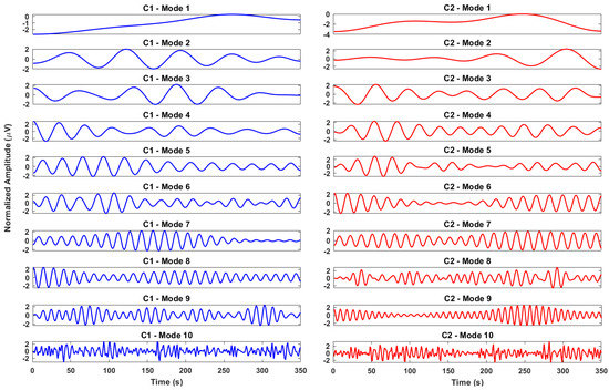
Figure 2. EFD modes for a sample trial of subject A1 using channel C3. C1 denotes class 1, while C2 indicates class 2 MI EEG task signal.

3.3. Step 3: Scalogram Transformation with Hilbert Transform (HT)

Following EFD decomposition, the time-changing signals are transformed into 2D scalogram representations. We use the Hilbert transform (HT) to obtain the Hilbert spectrum of time-varying signals for this purpose. The Hilbert spectrum is the result of a two-step process in which the non-stationary EEG is first decomposed into stationary sub-band signals, and then the HT for each sub-band is computed in order to obtain instantaneous frequencies. A single channel EEG signal z(t) can be described mathematically as a linear combination of its EFD IMFs as follows:

$$z\left(t\right)=\sum _{i=1}^M{q}_i\left(t\right)$$

(8)

where M is the EFD decomposition level and $q_i\left(t\right)$ is the i-th EFD IMF. Every single IMF can be further represented as follows:

$$q_i\left(t\right)=\mathbb{R}\left\{b_i\left(t\right)e^{-i{\theta }_i\left(t\right)}\right\}=b_i\left(t\right)cos\left({\theta }_i\left(t\right)\right)$$

(9)

where $b_i\left(t\right)$ is the Fourier series coefficients, and ${\theta }_i\left(t\right)$ is the phase of $q_i\left(t\right)$. The instantaneous frequency for i-th EFD IMF could then be defined as:

$${\Omega }_i\left(t\right)=\frac{d{\theta }_i\left(t\right)}{dt}$$

(10)

Consequently, the Hilbert spectrum for $q_i\left(t\right)$ can be defined as:

$$H_i\left(\Omega ,t\right)=\left\{\begin{array}{c}{b}_j\left(t\right),\Omega ={\Omega }_i\left(t\right)\hfill \\ 0,Otherwise\hfill \end{array}\right.$$

(11)

Finally, the Hilbert spectrum for z(t) could be constructed as:

$$H\left(\Omega ,t\right)=\sum _{i=1}^M{H}_i\left(\Omega ,t\right)$$

(12)

The singular vectors of the Hilbert transform yield transient harmonics that are time functions, resulting in an energy distribution over frequency and time. Figure 3 illustrates the sample EFD scalograms using the Hilbert spectrum technique. The Hilbert spectrum is significant in several ways for the existing EFD-CNN analysis: first, it is a non-parametric technique for converting time-dependent 1D signals into 2D time-frequency representation without any pre-defined constraints; second, it is computationally efficient and operates linearly over the input EEG signal; third, Hilbert spectrum gives an exceptional time-frequency amalgamation contrary to wavelet analysis, which fails to localize the frequency and energy robustly. Conclusively, the contemplated virtues of the HT method suggest its efficacy be adopted in the ongoing study.

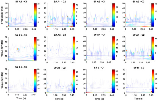
Figure 3. Hilbert spectrum for EFD modes for class 1 (C1) and class 2 (C2) activities utilizing MI EEG recordings from participants A1–A5 and B.

3.4. Step 4: Feature Extraction and Classification with Pre-Trained Convolutional Neural Network Models

Convolutional neural network (CNN) models have seen a meteoric rise in popularity in recent image classification-based research due to their remarkable self-feature extraction ability. Layers in a CNN may either be used for feature extraction or categorization. The layered architecture of the CNN model could be classified into two distinct categories: features extractions layers, and classification layers, based on their working functionality. The feature extraction layers consist of convolutional, activation function, pooling, and batch normalization layers. At the same time, the classification layers are formed by combining fully connected, dropout, softmax, and output layers accordingly. The feature extraction layers quantify geometrical patterns in an image, such as edges, textures, forms, and objects, and send them to the classification layers, which make the ultimate determination about the class label.

The downside of using CNN-based algorithms is that they are time-consuming and computationally expensive. Pretrained networks, on the other hand, do not need training a CNN from the start; instead, a model trained on millions of pictures may be modified to accommodate a new purpose. Transfer learning is fine-tuning a pre-trained network to execute or learn an unfamiliar job. Four small- and medium-scale pre-trained CNN models—AlexNet, SqueezeNet, ShuffleNet, and GoogLeNet—were examined in this work to find the optimum model for motor imagery EEG categorization issues. Table 2 briefly describes the characteristics of the four pre-trained models used in the present study.

Table 2. Summarized description of pre-trained CNN models.

Pre-Trained CNN Model	No. of Layers	Input Dimensions	Replaceable Final Layers	No. of Parameters in the Replaceable Layers
AlexNet	25	$227\times 227$	fc8, prob, output	8194
SqueezeNet	68	$227\times 227$	Pool10, prob, ClassificationLayer_predictions	1026
ShuffleNet	173	$224\times 224$	Node_202, softmax, ClassificationLayer_node_203	1090
GoogleNet	144	$224\times 224$	Loss3-classifier, prob, output	2050

4. Experimental Arrangements

This module elucidates the empirical configuration for the devised EFD-CNN mechanism. Specifically, we narrate the input-output arrangements for dataset 1 EEG signals type; however, a similar process could be extended to dataset 2, 3, and 4 signals. Figure 4 illustrates a pictorial representation of the designed EFD-CNN workflow. At first, the single-trial EEG signals with dimension 350 × 118 (where 350 is the signal length and 118 is the number of EEG electrodes) is subjected to MSPCA denoising, yielding a denoised 350 × 118 matrix. Since the denoising process solely affects the magnitude of signals, there is no dimensional alteration between the input-output matrices. Next, the excessive number of channels is discarded by selecting the 18 most significant channels. Those channels are $C_5,C_3,C_1,C_2,C_4,C_6,C{P}_5,C{P}_3,C{P}_1,C{P}_2,C{P}_4,C{P}_6,P_1,P_3,P_1,P_2,P_4$, and $P_6$, accordingly. Since the sensory-motor cortex of the brain is where the MI EEG is expressed chiefly, it is crucial to choose a small number of electrodes that will contribute the most to the segregation of the MI EEG tasks. Our prior essay outlined the rationale and importance of choosing these 18 channels [25].

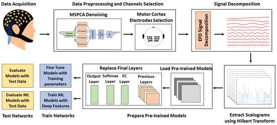
Figure 4. Block diagram of the proposed EFD-CNN framework.

After channel selection, the remaining single-trial EEG data matrix has the dimension 350 × 18. Next, the EFD is rendered for each channel of the resulting EEG matrix, where every column is decomposed into ten stationary intrinsic mode functions (IMFs). The decomposition level is obtained empirically by testing with a variable number of IMFs and evaluating their categorization ability. Further specifics about the EFD decomposition level selection will be explored in the results and discussions section. The EFD decomposition step gives a 350 × 10 × 18 tensor. Following, each 350 × 10 × C tensor (where C is a scalar value denoting the channel index) is subjected to HT to convert the time-varying signals into time-frequency scalograms, where each scalogram is an RGB image with dimension 543 × 429 × 3. Likewise, we retrieve 18 scalograms for a single trail EEG signal. The aforesaid process is iterated for all trails belonging to different classes until all the time-varying signals are transformed into RGB scalograms. Finally, the scalograms are reshaped according to the input requirements of each pre-trained CNN model, and then the AlexNet, ShuffleNet, SqueezeNet, and GoogleNet models are iteratively fine-tuned over the EFD scalograms. As per the best practices explored by our previous study [25] and another well-reputed research [34], the fine-tuning parameters are designated as follows: learning rate = $1\times {10}^{-4}$, optimizer = root mean square propagation (RMSProp), batch size = 64, and no. of epochs = 15.

The classification performance is gauged using the accuracy, f1-score (f-measure), and Cohen’s kappa coefficient metrics. The accuracy of a classification system is measured as the percentage of correct classifications relative to the total number of examples. This is an essential metric for assessing a classification model’s overall performance; however, it is insufficient when dealing with lopsided and skewed datasets. The f-measure is a performance statistic calculated by taking the harmonic mean of the precision and recall measures. The f-measure considers the data imbalance and makes an unbiased judgment. A higher f1-score indicates improved categorization performance and vice versa. Cohen’s kappa, or simply kappa, is a qualitative attribute for measuring the inter-rater reliability of the classifier. The kappa coefficient helps determine the validity of various classification and testing methods.

The computational setup for the experimental procedure involves Intel (R) i7-9750H CPU @ 4.5GHz processor, Windows 11 64-bit operating system with 16GB RAM, and Nvidia RTX 2060 GPU with 6GB GDDR6 type memory using MATLAB R2022a software. All the experiments in this research study are conducted exercising the 10-fold cross-validation strategy in which the entire dataset is subdivided into ten equal portions. Nine data segments are combined to form a training set, while one segment is kept for model evaluation. In this way, every single trial acts both as a training and testing sample subsequently.

5. Results and Discussions

This section describes the empirical examination of the proposed EFD-CNN framework. To assess the robustness of the suggested approach, we created several subject-dependent and independent case scenarios across four large- and small-scale datasets. It should be noted that, unless otherwise stated, the classification performance for the best-case AlexNet CNN model upon dataset 1 and 2 subjects is presented for general evaluation.

5.1. A. 10-Fold Performance Evaluation

This section evaluates the quantitative results for the proposed EFD-CNN scheme pertaining to accuracy, f1-score, kappa, and confusion charts. Figure 5 shows the statistical evaluation of classification results in the form of box plots. The box plots are essential for illustrating the generic group response of a data distribution, where the center line in the box depicts the median value, the lower and upper boundaries of the box illustrate the 1st and 3rd quartiles, while the side whiskers denote the minimum and maximum values of the distribution.

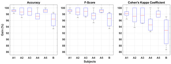
Figure 5. Box plot of 10-fold performance metrics obtained from the devised classification model for all subjects of datasets 1 and 2.

First, we quantify the 10-fold accuracy, f1-score, and kappa coefficient employing the box plot practice. It can be seen that the median accuracy and f1-score for all subjects is >96%, while the kappa coefficient is >95% for subjects A1–A5 and >92% for subject B. Next, the interquartile range (IQR) considering the accuracy and f1-score metric for subjects A1–A5 is <3%, and for subject B is <4% without any considerable side whiskers (extrema), indicating a low heterogeneity across the 10-folds. The IQR variations for the kappa coefficient are <5–6% for all subjects, demonstrating a strong inter-observer agreement. Furthermore, the mean accuracies for subjects A1–A5 and B are 99.10%, 98.70%, 98.80%, 97.50%, 99.05%, and 96.03% accordingly. Similarly, the mean f1-score values are 99.10%, 98.70%, 98.73%, 97.45%, 99.06%, and 96.36%, respectively. Lastly, the average kappa scores are 98.20, 97.40%, 97.57%, 94.91%, 98.08%, and 92.65% accordingly.

The confusion matrices pertaining to the classification performance of dataset 1 and 2 subjects employing the proposed EFD-CNN method are illustrated in Figure 6. A confusion matrix is distinctively efficacious for performance evaluation since it gives adequate exposure to the classification outcomes of imbalanced datasets. The figure shows that the false positive (FP) and false negative (FN) rate is <3% for subjects A1, A2, A3, A4, and B, whereas for subject A5, it is <4%. This is because subject A5 only has 27 classification instances, while only one sample was misclassified. The sensitivity, specificity, and precision coefficients are >96% for all subjects, testifying to the robustness of the envisaged EFD-CNN model. The accumulative quantitative analytics reveals that our method has achieved promising classification performance with interrater reliability, a non-complex and automated signal processing model capable of dealing with balanced and imbalanced EEG datasets simultaneously.

Figure 6. Confusion charts based on the classification results obtained from proposed EFD-CNN for all subjects of dataset 1 and 2.

5.2. B. Effect of Varying Number of EFD Modes

This section unravels the EFD decomposition level (M)’s impact on the classification success rate. As described in section III.B, the EFD method has a single tunable parameter M, which defines the number of decomposed stationary sub-bands or simply IMFs. The IMFs are arranged in ascending order of frequency, each containing a band-limited stationary signal. A lower value of M denotes a low decomposition level and wideband IMFs, while a higher value indicates a greater decomposition and narrowband IMFs. We are interested to see whether the M-factor contributes to increasing or decreasing the classification outcomes. Figure 7 illustrates the empirical results for this particular scenario, where the M-factor in the EFD-CNN framework is tuned between [1, 50] for all subjects of datasets 1 and 2, and the classification accuracy is observed for each case.

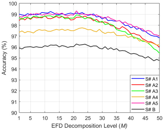
Figure 7. Effect of changing EFD decomposition level (M) on subject categorization in datasets 1 and 2.

It can be seen in Figure 7 that the average accuracy undergoes a slight increment for the range 1 ≤ M < 20. For M ≥ 20, the accuracy diminishes by 3% on average for all subjects, escalating the misclassification rate. It is also observed that the success rate varies <1% between the range 10 ≤ M ≤ 20. Since a higher decomposition level requires more time to calculate IMFs and also the average accuracy is stable between the interval [10,20]; therefore we choose M = 10 as a tradeoff value between the classification performance and computational expense. The performance diminution for M ≥ 20 is that the bandwidth for each IMF keeps getting narrower upon the increase in M-factor. The Hilbert spectrum fails to adequately maintain the ERD/ERS information of the signals, resulting in a blurring of the classification boundary between two MI EEG tasks and worse classification performance. The current experiment also validates our previous study [19], in which a similar experiment was carried out utilizing traditional signal processing methods. A similar conclusion was reached in that example, where classification accuracy decreased as the decomposition level increased. This study also confirms that the same conclusion holds for time-frequency images and that EFD performance is insensitive to the input signal transformation.

5.3. C. Performance Comparison with Other SD Methods

We further compare the acquired findings with various benchmark signal decomposition (SD) methods in the EEG domain in order to accurately assess the proposed EFD-CNN model classification performance. Such techniques incorporate variational mode decomposition (VMD), multivariate variational mode decomposition (MVMD), empirical mode decomposition (EMD), empirical wavelet decomposition (EWT), tunable-Q wavelet transform (TQWT), and wavelet packet decomposition (WPD). Although they each have their own unique set of clinical drawbacks, these techniques have found widespread use in EEG data analysis for various purposes. To provide a more accurate comparison between these techniques and our proposed EFD-CNN scheme, we merged them with the AlexNet CNN model in this section.

The classification accuracy for various SD-CNN techniques is shown in Table 3. It has been found that the suggested EFD-CNN technique surpasses all other SD-CNN methods conclusively, resulting in an average accuracy of 98.2% for all subjects of datasets 1 and 2. Subsequently, VMD is placed second with an average success rate of 97.7%. The difference between EFD-CNN and VMD-CNN is only 0.42%, which is minor; nonetheless, the inherent disadvantage of VMD (as explained in the introductory section) makes it unsuitable for MI EEG analysis. The average success score for MVMD-CNN, EMD-CNN, EMD-CNN, and TQWT-CNN is greater than 90%; however, the performance gap between these methods and our suggested technique is greater than 2%, which is a significant account. Finally, the WPD-CNN model earned the lowest average classification score of 88.5%, roughly 10% lower than the recommended EFD-CNN. Overall, the EFD method outperforms classic SD methods in qualitative and quantitative outputs.

Table 3. EFD-CNN performance comparison with other SD-CNN methods for all subjects of dataset 1 and 2.

SD. Methods	A1	A2	A3	A4	A5	B	Average
EFD-CNN	99.10	98.70	98.80	97.50	99.05	96.03	98.20
VMD-CNN	99.91	98.61	97.93	97.41	98.68	95.13	97.78
MVMD-CNN	96.38	96.25	96.76	95.46	96.21	94.00	95.84
EMD-CNN	96.06	95.19	95.60	93.64	95.47	92.95	94.82
EWT-CNN	94.89	94.66	94.46	92.54	94.90	91.96	93.90
TQWT-CNN	92.78	92.46	92.54	90.89	92.71	89.20	91.76
WPD-CNN	89.81	88.73	89.08	87.55	89.15	86.85	88.53

5.4. D. Results with Other Pre-Trained CNN Models

In addition to selecting an acceptable EFD decomposition level, selecting an appropriate pre-trained CNN model is critical for effective MI EEG categorization. The selection criteria for such models include improved classification accuracy and minimal computational complexity. Our earlier study in [25] examined ten large- and small-scale CNN models for MI EEG segregation, and it was determined that the AlexNet, ShuffleNet, SqueezeNet, and GoogleNet CNN frameworks serve our two principles for model selection. Figure 8 exhibits comparison bar graphs for classification accuracy using the pre-trained models. It is observed that AlexNet achieves the highest success score of 99.1%, 98.7%, and 98.8% for subjects A1, A2, and A3, respectively, while for subjects A5 and B, ShuffleNet yields the highest classification accuracy of 99.5% and 96.8%. However, the difference between ShuffleNet and AlexNet classification performance is <1%, which could be neglected. The minimum success rate was obtained with GoogleNet, yielding 97.6%, 96.9%, 96.3%, 96.8%, 99%, and 94.6% accuracies for dataset 1 and 2 subjects. Most of the outcomes are >90% and demonstrate MI EEG signals to have a promising capacity for classification. AlexNet has been chosen as the best-performing model and is generally considered for the entire analysis in this study due to its low complexity, and fewer layers.

Figure 8. Performance comparison for various pre-trained CNN models in combination with EFD method using dataset 1 and 2 subjects.

5.5. E. Deep Features Extraction and Classification with Machine Learning Methods

The capacity of CNN models to extract their own features has dramatically increased the idea of deep feature extraction from CNN models and categorization with machine learning. This section aims to examine a case scenario in which the deep EFD features are extracted from a fine-tuned AlexNet model and classified with four machine learning (ML) classifiers, including support vector machine (SVM), k-nearest neighbor (kNN), decision tree (DT), and logistic model tree (LMT) classifiers, respectively. The parameters for the aforementioned ML classifiers have been left unchanged from those examined in our prior study [22], where a thorough performance comparison in conjunction with the varied ML model parameters was carried out.

The differences in classification accuracy between the proposed EFD-CNN model and the other four EFD-ML approaches are shown in Figure 9. It is clear that our suggested strategy performs better than other ML models by a margin of at least 9%. EFD-SVM had the best accuracy of any ML model, with success scores of 90.7%, 90.5%, 89%, 89.3%, 90.3%, and 86.2% for subjects A1–A5, and B, respectively. EFD-SVM is followed by EFD-kNN relenting 88.6%, 88.7%, 89.7%, 88.4%, 88.3%, and 86.9% classification scores, respectively, for the aforesaid subjects. The minimum accuracy is reported by EFD-LMT, giving 87.1%, 87.1%, 86.6%, 84%, 87.2%, and 84.3% success scores for dataset 1 and 2 subjects. According to the overall empirical findings, fully connected layers in the AlexNet-CNN model accurately estimate the input-output mapping function for multitask MI EEG EFD scalograms and pinpoint the real boundary between the deep features. However, the ML models are unable to achieve this either due to the high dimensionality of the deep features or the enormous volume of training data. If the goal is features analysis rather than classification performance, however, several dimensionality reduction methods [8] and post-processing approaches [22] could be used to examine the deep features and draw conclusions about the MI EEG signals.

Figure 9. EFD-CNN evaluation against deep features extracted from AlexNet CNN model and classified with different machine learning classifiers.

5.6. F. Comparison with Other State-of-the-Art Studies

To further investigate the performance and utility of the proposed EFD-CNN scheme, the classification accuracies of dataset 1 subjects are contrasted against well-reputed contemporary methods. Table 4 catalogs 14 studies that employed either conventional signal processing techniques or automated deep learning frameworks for dataset 1 MI EEG classification. It can be seen that the proposed EFD-CNN method ranks second among our comparative studies with an overall average accuracy of 98.6%, whereas our previous study [19] is positioned at the top of the list with an average success score of 99.8%. The performance discrepancy is merely 1.2% which is not significant considering the utilities of the EFD-CNN model, such as simplex architecture, automatic feature extraction, performance invariance for multiple datasets, and promising performance for subject-independent case scenarios. Advancing, the study in [35] exploited an AlexNet-based classification framework incorporating Fourier transform (FT), common spatial patterns (CSP), discrete cosine transform (DCT), and empirical mode decomposition (EMD) for 3D scalogram construction. The proficiency of such a model is satisfactory, with an average accuracy of 98.5%. Yet, the adopted architecture is too complex and necessitates multiple time-frequency resolution methods to attain an identical performance that we achieved with a single SD technique.

Table 4. EFD-CNN performance comparison with state-of-the-art studies for dataset 1.

Authored by	Proposition	A1	A2	A3	A4	A5	Average
Our Previous Study [19]	EFD + IEFD + Welch PSD + FFNN	99.9	99.8	99.9	99.8	100	99.8
This study	EFD-CNN	99.1	98.7	98.8	97.5	99	98.6
Taheri et al. [35]	FT + CSP + DCT + EMD + AlexNet	100	97.6	98.8	96.4	100	98.5
Sadiq et al. [34]	MEWT + JIA + LS-SVM	95	95	95	100	100	97
Siuly et al. [36]	EMD + AIMF Features + LS-SVM	97.7	98.8	96.6	98.8	95.5	97.5
Siuly et al. [37]	OA + NB	97.9	97.8	98.2	94.4	93.2	96.3
Siuly et al. [38]	CC + LS-SVM	97.8	99.1	98.7	93.4	89.3	95.7
Sadiq et al. [16]	EWT + IA2 + LS-SVM	94.5	91.7	97.2	95.6	97	95.2
Fang et al. [39]	ESI + CWT + CNN	89.9	98.8	90.6	95.6	91.2	93.2
Miao et al. [40]	CNN based on frequency characteristics of MI EEG	100	90	90	90	80	90
Kevric et al. [41]	WPD + Statistical Features + kNN	77.1	72.2	75.2	85.6	86	79.2
Lotte at al. [42]	SSRCSP	70.5	96.4	53.5	71.8	75.3	73.5
Lotte et al. [42]	TRCSP	71.4	96.4	63.2	71.8	86.9	77.9
Lotte at al. [42]	WTRCSP	72.3	96.4	60.2	77.4	86.5	78.6
Kevric et al. [41]	DWT + Statistical Features + k-NN	56.6	60.7	55.9	55.1	90.1	63.6

The studies in [16,34,36,37,38] embraced conventional signal processing methods with handcrafted features in order to achieve >95% classification scores. Nevertheless, their difference in accuracy with the proposed scheme is >2%; also, the processing frameworks are complicated to perceive. The studies in [39,40] also deploy CNN-based architectures; however, they produce an accuracy deficit of 5.4% and 8.6%, respectively. The minimum classification accuracy in the entire table was reported by [41], which is 63.6% using the discrete wavelet transform (DWT), statistical features, and kNN classifier. We observe that our model achieves a maximum of 35% increment in classification performance compared to the lowest-performing model, which is a significant improvement considering a non-complex and fully automated architecture. We would like to clarify that the existing comparative study does not discuss a 1D-CNN model or those deep learning methods explicitly designed for EEG problems, such as EEGNet [29], deep ConvNet [28], and 1D ConvNet [30]. This is because those models are still in the research phase and do not yield promising classification performance despite being physiologically significant for MI EEG signals. The overall analysis concludes that our EFD-CNN model subjugates other existing signal processing models in terms of classification performance and simplex architecture.

5.7. G. Empirical Results for Dataset 3

One predominant problem connected with such MI EEG classification models in contemporary research is that they are highly prone to inter-subject variations and acquisition techniques, and their application is restricted to small datasets with a few subjects. We investigate the usefulness of our proposed EFD-CNN model for a large dataset 3 with 52 participants to demonstrate its robustness against inter-subject variations. The dataset contains MI EEG signals from 38 well-discriminative and 13 less-discriminative participants, giving rise to a challenge of inter-subject variance and the hypersensitive classification ability of the designed framework.

The empirical findings for dataset 3 participants using the EFD-CNN model are given in Table 5. A detailed analysis of the results shows that the proposed model produces an overall f1-score and average accuracy of 89.9%. The kappa coefficient is 79.8%, significantly higher than the minimum threshold of 70% required for a BCI system. Further analysis reveals that the accuracy rate is >90% for 26 participants, between 85 and 90% for 17 subjects, and 80–85% for 11 participants, respectively. This is especially intriguing when compared to the results of other investigations. We notice that the study in [25] produced an average accuracy of 87.6%, with only 18 people scoring above 90%, 12 subjects scoring between 85 and 90%, and 19 participants scoring between 80 and 85%. The minimum results obtained by EFD-CNN for any subject in dataset 3 are 80.03%, compared to 78.54% [25], 73.06% [43], 72.15% [31], and 25.42% [44] reported by its counterparts. This section concludes that the EFD-CNN method is independent of inter-subject transfer and robust for a wide range of MI EEG datasets with different acquisition protocols.

Table 5. EFD-CNN performance evaluation and comparison for all subjects of dataset 3.

Subjects	Performance Metrics			Performance Comparison
	Accuracy	F1-Score	Kappa	Sadiq	Sadiq	Yu	Kumar
	(%)	(%)	(%)	et al. [25]	et al. [43]	et al. [31]	et al. [44]
S01	94.17	94.57	88.27	90.79	87.69	82.5	80
S02	85.83	85.95	71.67	91.38	90.6	85.48	52.33
S03	99.17	99.22	98.32	94.88	95.68	95.71	94
S04	93.33	93.44	86.72	91.58	87.68	83.52	78
S05	100	100	100	100	99.06	98.58	99
S06	96.67	96.67	93.34	92.69	89.03	86.51	82.33
S07	82.5	80.37	64.71	84.71	81.83	79.5	52.78
S08	87.5	86.73	74.92	82.55	79.85	78.55	55.67
S09	89.17	86.02	77.18	82.17	79.23	82.55	56.4
S10	92.5	93.13	84.88	89.65	86.65	80.52	73
S11	82.5	82.05	64.98	82.75	76.03	75.56	57.33
S12	90	91.18	79.64	83.22	78.44	80.53	67.17
S13	94.17	94.31	88.33	91.21	89.01	94.58	84.5
S14	100	100	100	100	98.02	97.57	96.5
S15	89.17	87.85	78.09	90.98	87.2	75.57	64.67
S16	83.33	85.07	66.22	82.85	77.49	81.54	47.5
S17	83.33	81.13	66.24	78.54	73.06	79.56	49.67
S18	80.83	82.44	61.37	81.31	77.07	77.58	53.33
S19	87.5	86.73	74.92	84.1	78.26	80.56	57.17
S20	91.67	91.38	83.32	88.8	85.42	77.53	72.83
S21	90.83	90.43	81.64	91.05	88.21	74.51	66
S22	87.5	87.8	75.03	82.91	79.03	78.58	58.67
S23	94.17	94.31	88.33	87.82	87.84	87.5	84.17
S24	84.17	83.76	68.33	81.94	78.22	79.55	60.67
S25	83.33	84.38	66.53	82.59	78.65	72.51	53
S26	99.17	99.2	98.33	100	99.04	98.56	96.83
S27	81.67	82.54	63.28	82.49	76.49	76.54	44.67
S28	95	95	90	92.23	91.43	78.6	80.83
S29	85	83.64	69.82	79.82	74.8	91.54	43
S30	87.5	86.24	74.83	87.78	86.64	76.51	55.5
S31	86.67	85.71	73.28	86.09	84.43	78.52	62.33
S32	88.33	88.71	76.64	86.12	83.66	77.56	50.57
S33	87.5	88.37	74.9	83.24	79.6	73.59	55.67
S34	85.83	85.95	71.67	84.09	77.65	80.52	58
S35	94.17	94.74	88.2	90.57	91.67	85.54	81.83
S36	88.33	89.55	76.34	84.88	83.7	82.53	69.5
S37	92.5	91.74	84.88	91.12	90.42	83.52	77
S38	84.17	84.55	68.42	83.1	79.1	77.6	48.5
S39	91.67	91.53	83.33	86.57	86.21	80.51	73
S40	83.33	83.33	66.68	82.51	75.81	77.54	51.17
S41	94.17	94.66	88.24	89.7	87.64	92.59	85.33
S42	86.67	85.45	73.18	81.4	74.64	75.54	48.33
S43	100	100	100	98.08	99.04	99.53	95.83
S44	97.5	97.3	94.97	92.85	93.29	94.53	89.17
S45	86.67	84.62	72.86	84.57	82.29	82.58	52.5
S46	85	86.15	69.82	79.49	75.89	85.57	25.42
S47	91.67	91.53	83.33	88.48	89.08	88.57	74.17
S48	91.67	92.96	82.76	89.67	89.21	90.53	78.17
S49	97.5	97.48	95	94.73	93.41	91.54	87.5
S50	100	100	100	99	100	98.58	100
S51	84.17	85.27	68.26	85.06	84.04	89.56	53.17
S52	89.17	89.6	78.3	85.71	82.69	84.54	61.83
Average	89.97	89.9	79.81	87.68	85.02	83.83	67.24

5.8. H. Empirical Results for Dataset 4

Further evaluation for the inter-subject invariance of the EFD-CNN is carried out using a three-class mental imagery EEG dataset 4, having distinct acquisition standards. The dataset has three participants, each performing three cued tasks repetitively. To further assess the relative performance of each class, we changed the multi-class classification issue into a binary class problem, as practiced by [19,45]. Table 6 depicts various case scenario arrangements in which each class is contrasted with the remaining two classes for each subject. As a result, nine different cases are formed, the empirical results of which are shown in Table 7.

Table 6. List of binary class combinations for dataset 4 subjects.

Subjects	Cases	Combinations
Subject 1	Case 1	Class 1 vs. Class 2
	Case 2	Class 1 vs. Class 3
	Case 3	Class 2 vs. Class 3
Subject 2	Case 4	Class 1 vs. Class 2
	Case 5	Class 1 vs. Class 3
	Case 6	Class 2 vs. Class 3
Subject 3	Case 7	Class 1 vs. Class 2
	Case 8	Class 1 vs. Class 3
	Case 9	Class 2 vs. Class 3

Table 7. EFD-CNN performance evaluation and comparison for all subjects of dataset 4.

Cases	Performance Metrics			Performance Comparison
	Accuracy	F1-Score	Kappa	Siuly	Sadiq
	(%)	(%)	(%)	et al. [45]	et al. [12]
Case 1	96.42	96.29	92.85	65.88	94.58
Case 2	92.85	95	82.5	75.35	91.16
Case 3	85.71	84.61	71.42	62.68	81.17
Case 4	98.98	97.97	95.99	58.95	100
Case 5	100	100	100	73.04	100
Case 6	85.71	81.81	70.05	62.35	82.15
Case 7	96.42	97.14	92.39	47.84	97.46
Case 8	99	99.01	97.99	51.47	99.16
Case 9	89.28	91.89	76.13	52.71	80.54
Average	93.81	93.74	86.65	61.14	91.8

It can be seen that the proposed method achieves an average accuracy of 93.8%, which is greater than the previously reported classification accuracies of 61.1% and 91.8% by [12,45], respectively. The results further highlight the suitability of the EFD-CNN method in terms of individual case outcomes, where our method significantly exceeds the prior studies. In some instances, previous approaches were more accurate than ours; nonetheless, the difference is less than 2%, which is regarded as inconsequential. In addition, the results reveal consistency between other performance measures and the accuracy metric. As can be observed, the mean, f1-score, and kappa coefficient are 93.7 and 86.6 percent, respectively. These findings validate our strategy’s consistency and inter-rater reliability for analyzing datasets with an uneven distribution. A closer look at the gathered results reveals that the f-measure and kappa coefficient are in perfect agreement with the classification accuracy. The current analysis concludes that the EFD-CNN framework is robust for the mental imagery EEG dataset in terms of above-average classification performance, surpassing previously reported results and stable outcomes for skewed datasets.

5.9. I. Subject-Independent Case Results

Subject-independent (SI) BCI systems emerged due to their remarkable capacity to generalize training information obtained from a specific set of subjects to a new user without the necessity for that user’s training data. Subject-dependent BCI systems provide several challenges in their implementation, such as computational complexity, portability, operational hassles, data collecting and training a model from scratch for a new user, etc. In this section, we extend the applicability of our EFD-CNN model to SI classification. For this purpose, dataset 1 is initially denoised with MSPCA, and 18 motor cortex channels are selected, similar to the subject-dependent case scenario. The subsequent dataset is then subjected to EFD decomposition, where ten EFD modes are extracted from every channel. Afterward, the 1D signals are transformed into 2D scalograms employing the HT method. Lastly, the scalograms are fed to the AlexNet pre-trained model for fine-tuning and classification. In this study, the AlexNet model is trained using 30 permutations of five subjects (A1, A2, A3, A4, and A5), and testing is carried out using the leave-one-subject-out (LOSO) strategy.

Table 8 illustrates the classification accuracies concerning the SI case scenario for dataset 1. It can be seen that subject A2 attains the maximum success rate of 87.02% for the target subject A5. Subjects A2, A3 (as source) and A1 (as target), A4, A5 (as source) while A1 (as target), A5 (as source) and A4 (as target), A2, A4 (as source) while A3 (as target) achieves approximately identical classification accuracy of 86+%. The minimum segregation outcomes of <70% were observed in the case of subjects A1, A3 (as source) and, A5 (as target), A5 (as source) while A2 as the target. All other combinations yield above 70% accuracy for all source subjects. To further extend the analysis, Figure 10 compares the average success scores achieved by individual combinations in Table X and the ones reported by our previous study [19] utilizing EFD+spectral features. For better clarity, the current outcomes are arranged in descending order of their achieved accuracies. In 29 instances, the suggested EFD-CNN model performs better than its predecessor. The EFD+spectral features model only produces one result with a score greater than >80% for Comb. 26, while it scores <70% in all other instances. Furthermore, the difference between the maximum and minimum performance scores by the EFD-CNN model is only 14.03% which is 2.8 times less than the EFD-spectral features model (having a 39.60% discrepancy between extrema).

Table 8. Subject independent case results for different training and testing data combinations using dataset 1 subjects.

Combination #	Subject	A1	A2	A3	A4	A5
	Combinations
Comb. 1	A1	-	77.74	72.9	83.46	79.79
Comb. 2	A2	82.24	-	83.08	83.62	87.06
Comb. 3	A3	69.89	79.24	-	72.03	74.82
Comb. 4	A4	86.02	83.43	84.82	-	86.46
Comb. 5	A5	82.27	69.82	72.45	86.78	-
Comb. 6	A1, A2	-	-	75.24	82.94	79.65
Comb. 7	A1, A3	-	72.56	-	85.64	69.11
Comb. 8	A1, A4	-	71.31	74.96	-	83.32
Comb. 9	A1, A5	-	86.7	83.63	72.47	-
Comb. 10	A2, A3	86.97	-	-	71.53	79.91
Comb. 11	A2, A4	83.17	-	86.74	-	71.86
Comb. 12	A2, A5	74.19	-	72.83	76.48	-
Comb. 13	A3, A4	81.55	81.86	-	-	77.55
Comb. 14	A3, A5	80.7	80.5	-	83.1	-
Comb. 15	A4, A5	86.81	78.37	86.12	-	-
Comb. 16	A1, A2, A3	-	-	-	80.55	74.22
Comb. 17	A1, A2, A4	-	-	73.5	-	71.77
Comb. 18	A1, A2, A5	-	-	75.43	76.09	-
Comb. 19	A1, A3, A4	-	80.08	-	-	80.36
Comb. 20	A1, A3, A5	-	78.68	-	72.45	-
Comb. 21	A1, A4, A5	-	70.02	72.27	-	-
Comb. 22	A2, A3, A4	83.57	-	-	-	79.51
Comb. 23	A2, A3, A5	73.54	-	-	73.55	-
Comb. 24	A2, A4, A5	74.5	-	78.17	-	-
Comb. 25	A3, A4, A5	81.49	78.19	-	-	-
Comb. 26	A1, A2, A3, A4	-	-	-	-	74.04
Comb. 27	A1, A2, A3, A5	-	-	-	76.11	-
Comb. 28	A1, A2, A4, A5	-	-	73.39	-	-
Comb. 29	A1, A3, A4, A5	-	74.51	-	-	-
Comb. 30	A2, A3, A4, A5	74.61	-	-	-	-

Figure 10. Performance evaluation and comparison of SI case with previously reported Ref. 1: [19] results.

The findings of SI classification demonstrate that certain combinations of individuals sacrifice outstanding classification performance while others do not achieve equivalent results. This is because SI-EEG categorization hinges on inter-subject correlated features. In certain circumstances, the correlation between two subjects is high, whereas, in others, it is poor. When strongly correlated individuals are combined to form a training dataset, the classification performance of the resulting set improves. Conversely, when uncorrelated subject data is combined with correlated subject data, the aggregate redundancy of the training set increases, resulting in a reduction in classification accuracy. The overall SI results produced with the EFD-CNN framework are more significant than the benchmark (>70%); nonetheless, there is still potential for improvement that could be further improved in future studies.

6. Future Work

The existing report scrutinized the efficacy of EFD-CNN for MI EEG signals, and it was deduced that the contemplated method has the potential to form a promising BCI system. However, certain prospects are worth investigating for future studies: (1). the idea of multidomain EEG systems is getting immense attention owing to their exceptional ability to provide a one-window solution to diverse EEG problems. There are efforts [22], addressing this challenge; however, once again, the catalyzed architectures were too complex and based on the conventional signal processing methods. The current investigation rectifies the drawbacks associated with existing signal processing methods and could be extended to developing a multidomain EEG classification system. (2). In this study, the selection of the number of channels is made manually based on the prior recommendations by other studies. A research study could be conducted to automate the channel selection process and select the minimum number of clinically relevant electrodes for classification performance augmentation. (3). The selection of EFD decomposition level was empirically determined to be ten as per the accuracy contribution rate experiment. However, this process could be further automated by altering the EFD method in order to achieve a self-operating BCI system without any considerable human intervention.

7. Conclusions

In conclusion, this paper proposes a robust and non-complex signal processing framework by amalgamating the EFD and pre-trained CNN models for MI EEG task identification. The objective of this study was to evaluate the newly proposed EFD method in tandem with deep learning methods to devise an automated and self-feature extracting mechanism. The new EFD-CNN framework operated over four large- and small-scale binary and tertiary-class MI EEG datasets for performance validation. Experimental outcomes revealed superior classification performance for multiple case studies under subject dependent criterion, outperforming the contemporary studies by a fair margin. Further experiments under the subject-independent paradigm showed a highly improved model compared to the previously proposed prototype, indicating the large-scale utility and subject-to-subject transfer of the trained model. The suggested EFD-CNN architecture improves upon the limitations of prior approaches to time-frequency resolution, provides a simple signal processing pipeline, and offers a robust solution for MI EEG signals, can be adopted as a reliable BCI system.

References

- Pfurtscheller, G.; Neuper, C.; Muller, G.; Obermaier, B.; Krausz, G.; Schlogl, A.; Scherer, R.; Graimann, B.; Keinrath, C.; Skliris, D.; et al. Graz-BCI: State of the art and clinical applications. IEEE Trans. Neural Syst. Rehabil. Eng. 2003, 11, 1–4. [Google Scholar] [CrossRef]
- Nicolas-Alonso, L.F.; Gomez-Gil, J. Brain computer interfaces, a review. Sensors 2012, 12, 1211–1279. [Google Scholar] [CrossRef]
- Lee, M.H.; Kwon, O.Y.; Kim, Y.J.; Kim, H.K.; Lee, Y.E.; Williamson, J.; Fazli, S.; Lee, S.W. EEG dataset and OpenBMI toolbox for three BCI paradigms: An investigation into BCI illiteracy. GigaScience 2019, 8, giz002. [Google Scholar] [CrossRef]
- Zhu, H.; Forenzo, D.; He, B. On the Deep Learning Models for EEG-Based Brain-Computer Interface Using Motor Imagery. IEEE Trans. Neural Syst. Rehabil. Eng. 2022, 30, 2283–2291. [Google Scholar] [CrossRef]
- Ma, T.; Li, Y.; Huggins, J.E.; Zhu, J.; Kang, J. Bayesian Inferences on Neural Activity in EEG-Based Brain-Computer Interface. J. Am. Stat. Assoc. 2022, 117, 1–12. [Google Scholar] [CrossRef]
- Manojprabu, M.; Dhulipala, V.S. Improved energy efficient design in software defined wireless electroencephalography sensor networks (WESN) using distributed architecture to remove artifact. Comput. Commun. 2020, 152, 266–271. [Google Scholar] [CrossRef]
- Dai, C.; Wang, J.; Xie, J.; Li, W.; Gong, Y.; Li, Y. Removal of ECG artifacts from EEG using an effective recursive least square notch filter. IEEE Access 2019, 7, 158872–158880. [Google Scholar] [CrossRef]
- Babu, P.A.; Prasad, K. Removal of ocular artifacts from EEG signals using adaptive threshold PCA and wavelet transforms. In Proceedings of the 2011 IEEE International Conference on Communication Systems and Network Technologies, Katra, India, 3–5 June 2011; pp. 572–575. [Google Scholar]
- Ding, K.; Xiao, L.; Weng, G. Active contours driven by region-scalable fitting and optimized Laplacian of Gaussian energy for image segmentation. Signal Process. 2017, 134, 224–233. [Google Scholar] [CrossRef]
- Wang, G.; Wang, Y.; Min, Y.; Lei, W. Blind Source Separation of Transformer Acoustic Signal Based on Sparse Component Analysis. Energies 2022, 15, 6017. [Google Scholar] [CrossRef]
- Gokgoz, E.; Subasi, A. Effect of multiscale PCA de-noising on EMG signal classification for diagnosis of neuromuscular disorders. J. Med. Syst. 2014, 38, 1–10. [Google Scholar] [CrossRef]
- Sadiq, M.T.; Yu, X.; Yuan, Z.; Aziz, M.Z.; Siuly, S.; Ding, W. A matrix determinant feature extraction approach for decoding motor and mental imagery EEG in subject specific tasks. IEEE Trans. Cogn. Dev. Syst. 2020, 14, 375–387. [Google Scholar] [CrossRef]
- Riaz, F.; Hassan, A.; Rehman, S.; Niazi, I.K.; Dremstrup, K. EMD-based temporal and spectral features for the classification of EEG signals using supervised learning. IEEE Trans. Neural Syst. Rehabil. Eng. 2015, 24, 28–35. [Google Scholar] [CrossRef] [PubMed]
- Xiao-Jun, Z.; Shi-qin, L.; Fan, L.j.; Yu, X.L. The EEG signal process based on EEMD. In Proceedings of the 2011 IEEE 2nd International Symposium on Intelligence Information Processing and Trusted Computing, Wuhan, China, 22–23 October 2011; pp. 222–225. [Google Scholar]
- Keerthi Krishnan, K.; Soman, K. CNN based classification of motor imaginary using variational mode decomposed EEG-spectrum image. Biomed. Eng. Lett. 2021, 11, 235–247. [Google Scholar] [CrossRef] [PubMed]
- Sadiq, M.T.; Yu, X.; Yuan, Z.; Fan, Z.; Rehman, A.U.; Li, G.; Xiao, G. Motor imagery EEG signals classification based on mode amplitude and frequency components using empirical wavelet transform. IEEE Access 2019, 7, 127678–127692. [Google Scholar] [CrossRef]
- Zhang, Y.; Liu, B.; Ji, X.; Huang, D. Classification of EEG signals based on autoregressive model and wavelet packet decomposition. Neural Process. Lett. 2017, 45, 365–378. [Google Scholar] [CrossRef]
- Taran, S.; Bajaj, V. Motor imagery tasks-based EEG signals classification using tunable-Q wavelet transform. Neural Comput. Appl. 2019, 31, 6925–6932. [Google Scholar] [CrossRef]
- Yu, X.; Aziz, M.Z.; Sadiq, M.T.; Fan, Z.; Xiao, G. A new framework for automatic detection of motor and mental imagery EEG signals for robust BCI systems. IEEE Trans. Instrum. Meas. 2021, 70, 1–12. [Google Scholar] [CrossRef]
- Roy, G.; Bhoi, A.; Bhaumik, S. A comparative approach for MI-based EEG signals classification using energy, power and entropy. IRBM 2022, 43, 434–446. [Google Scholar] [CrossRef]
- Namazi, H.; Ala, T.S.; Kulish, V. Decoding of upper limb movement by fractal analysis of electroencephalogram (EEG) signal. Fractals 2018, 26, 1850081. [Google Scholar] [CrossRef]
- Yu, X.; Aziz, M.Z.; Sadiq, M.T.; Jia, K.; Fan, Z.; Xiao, G. Computerized Multidomain EEG Classification System: A New Paradigm. IEEE J. Biomed. Health Inform. 2022, 26, 3626–3637. [Google Scholar] [CrossRef]
- Sadiq, M.T.; Yu, X.; Yuan, Z.; Aziz, M.Z. Identification of motor and mental imagery EEG in two and multiclass subject-dependent tasks using successive decomposition index. Sensors 2020, 20, 5283. [Google Scholar] [CrossRef] [PubMed]
- Gaur, P.; Gupta, H.; Chowdhury, A.; McCreadie, K.; Pachori, R.B.; Wang, H. A sliding window common spatial pattern for enhancing motor imagery classification in EEG-BCI. IEEE Trans. Instrum. Meas. 2021, 70, 1–9. [Google Scholar] [CrossRef]
- Adem, Ş.; Eyupoglu, V.; Ibrahim, I.M.; Sarfraz, I.; Rasul, A.; Ali, M.; Elfiky, A.A. Multidimensional in silico strategy for identification of natural polyphenols-based SARS-CoV-2 main protease (Mpro) inhibitors to unveil a hope against COVID-19. Comput. Biol. Med. 2022, 145, 105452. [Google Scholar] [CrossRef] [PubMed]
- Mao, W.; Fathurrahman, H.; Lee, Y.; Chang, T. EEG Dataset Classification Using CNN Method; Journal of Physics: Conference Series; IOP Publishing: Bristol, UK, 2020; Volume 1456, p. 012017. [Google Scholar]
- Baygin, M.; Dogan, S.; Tuncer, T.; Barua, P.D.; Faust, O.; Arunkumar, N.; Abdulhay, E.W.; Palmer, E.E.; Acharya, U.R. Automated ASD detection using hybrid deep lightweight features extracted from EEG signals. Comput. Biol. Med. 2021, 134, 104548. [Google Scholar] [CrossRef] [PubMed]
- Behncke, J.; Schirrmeister, R.T.; Burgard, W.; Ball, T. The signature of robot action success in EEG signals of a human observer: Decoding and visualization using deep convolutional neural networks. In Proceedings of the 2018 IEEE 6th International Conference on Brain-Computer Interface (BCI), Gangwon, Republic of Korea, 15–17 January 2018; pp. 1–6. [Google Scholar]
- Jordanić, M.; Rojas-Martinez, M.; Mananas, M.A.; Alonso, J.F. Prediction of isometric motor tasks and effort levels based on high-density EMG in patients with incomplete spinal cord injury. J. Neural Eng. 2016, 13, 046002. [Google Scholar] [CrossRef]
- Giudice, M.L.; Varone, G.; Ieracitano, C.; Mammone, N.; Bruna, A.R.; Tomaselli, V.; Morabito, F.C. 1D Convolutional Neural Network approach to classify voluntary eye blinks in EEG signals for BCI applications. In Proceedings of the 2020 IEEE International Joint Conference on Neural Networks (IJCNN), Glasgow, UK, 19–24 July 2020; pp. 1–7. [Google Scholar]
- Yu, X.; Aziz, M.Z.; Hou, Y.; Li, H.; Lv, J.; Jamil, M. An Extended Computer Aided Diagnosis System for Robust BCI Applications. In Proceedings of the 2021 IEEE 9th International Conference on Information, Communication and Networks (ICICN), Xi’an, China, 25–28 November 2021; pp. 475–480. [Google Scholar]
- BCI Competition III. 2022. Available online: http://www.bbci.de/competition/iii/ (accessed on 13 October 2022).
- Zhou, W.; Feng, Z.; Xu, Y.; Wang, X.; Lv, H. Empirical Fourier Decomposition: An Accurate Adaptive Signal Decomposition Method. arXiv 2020, arXiv:2009.08047. [Google Scholar]
- Sadiq, M.T.; Yu, X.; Yuan, Z.; Zeming, F.; Rehman, A.U.; Ullah, I.; Li, G.; Xiao, G. Motor imagery EEG signals decoding by multivariate empirical wavelet transform-based framework for robust brain–computer interfaces. IEEE Access 2019, 7, 171431–171451. [Google Scholar] [CrossRef]
- Taheri, S.; Ezoji, M. EEG-based motor imagery classification through transfer learning of the CNN. In Proceedings of the 2020 IEEE International Conference on Machine Vision and Image Processing (MVIP), Qom, Iran, 18–20 February 2020; pp. 1–6. [Google Scholar]
- Taran, S.; Bajaj, V.; Sharma, D.; Siuly, S.; Sengur, A. Features based on analytic IMF for classifying motor imagery EEG signals in BCI applications. Measurement 2018, 116, 68–76. [Google Scholar] [CrossRef]
- Wang, H.; Zhang, Y. Detection of motor imagery EEG signals employing Naïve Bayes based learning process. Measurement 2016, 86, 148–158. [Google Scholar]
- Siuly, S.; Li, Y. Improving the separability of motor imagery EEG signals using a cross correlation-based least square support vector machine for brain–computer interface. IEEE Trans. Neural Syst. Rehabil. Eng. 2012, 20, 526–538. [Google Scholar] [CrossRef]
- Fang, T.; Song, Z.; Zhan, G.; Zhang, X.; Mu, W.; Wang, P.; Zhang, L.; Kang, X. Decoding motor imagery tasks using ESI and hybrid feature CNN. J. Neural Eng. 2022, 19, 016022. [Google Scholar] [CrossRef] [PubMed]
- Miao, M.; Hu, W.; Yin, H.; Zhang, K. Spatial-frequency feature learning and classification of motor imagery EEG based on deep convolution neural network. Comput. Math. Methods Med. 2020, 2020, 1981728. [Google Scholar] [CrossRef] [PubMed]
- Kevric, J.; Subasi, A. Comparison of signal decomposition methods in classification of EEG signals for motor-imagery BCI system. Biomed. Signal Process. Control 2017, 31, 398–406. [Google Scholar] [CrossRef]
- Lotte, F.; Guan, C. Regularizing common spatial patterns to improve BCI designs: Unified theory and new algorithms. IEEE Trans. Biomed. Eng. 2010, 58, 355–362. [Google Scholar] [CrossRef] [PubMed]
- Sadiq, M.T.; Yu, X.; Yuan, Z.; Aziz, M.Z.; Siuly, S.; Ding, W. Toward the development of versatile brain–computer interfaces. IEEE Trans. Artif. Intell. 2021, 2, 314–328. [Google Scholar] [CrossRef]
- Kumar, S.; Sharma, A.; Tsunoda, T. Brain wave classification using long short-term memory network based optical predictor. Sci. Rep. 2019, 9, 9153. [Google Scholar] [CrossRef]
- Li, Y.; Wen, P.P. Clustering technique-based least square support vector machine for EEG signal classification. Comput. Methods Programs Biomed. 2011, 104, 358–372. [Google Scholar]
Publisher’s Note: MDPI stays neutral with regard to jurisdictional claims in published maps and institutional affiliations. |
© 2022 by the authors. Licensee MDPI, Basel, Switzerland. This article is an open access article distributed under the terms and conditions of the Creative Commons Attribution (CC BY) license (https://creativecommons.org/licenses/by/4.0/).